Fusion of Various Band Selection Methods for Hyperspectral Imagery


1
Center for Hyperspectral Imaging in Remote Sensing, Information and Technology College, Dalian Maritime University, Dalian 116026, China
2
State Key Laboratory of Integrated Services Networks (Xidian University), Xi’an 710000, China
3
School of Physics and Optoelectronic Engineering, Xidian University, Xi’an 710000, China
4
The Remote Sensing Signal and Image Processing Laboratory, Department of Computer Science and Electrical Engineering, University of Maryland, Baltimore, MD 21250, USA
5
Department of Computer Science and Information Management, Providence University, Taichung 02912, Taiwan
*
Author to whom correspondence should be addressed.
Remote Sens. 2019, 11(18), 2125; https://doi.org/10.3390/rs11182125
Submission received: 12 July 2019
/
Revised: 22 August 2019
/
Accepted: 25 August 2019
/
Published: 12 September 2019
(This article belongs to the Special Issue Quality Improvement of Remote Sensing Images)
Abstract
:This paper presents an approach to band selection fusion (BSF) which fuses bands produced by a set of different band selection (BS) methods for a given number of bands to be selected, nBS. Since each BS method has its own merit in finding the desired bands, various BS methods produce different band subsets with the same nBS. In order to take advantage of these different band subsets, the proposed BSF is performed by first finding the union of all band subsets produced by a set of BS methods as a joint band subset (JBS). Due to the fact that a band selected by one BS method in JBS may be also selected by other BS methods, in this case each band in JBS is prioritized by the frequency of the band appearing in the band subsets to be fused. Such frequency is then used to calculate the priority probability of this particular band in the JBS. Because the JBS is obtained by taking the union of all band subsets, the number of bands in the JBS is at least equal to or greater than nBS. So, there may be more than nBS bands, in which case, BSF uses the frequency-calculated priority probabilities to select nBS bands from JBS. Two versions of BSF, called progressive BSF and simultaneous BSF, are developed for this purpose. Of particular interest is that BSF can prioritize bands without band de-correlation, which has been a major issue in many BS methods using band prioritization as a criterion to select bands.
1. Introduction
Hyperspectral imaging has emerged as a promising technique in remote sensing [1] due to its use of hundreds of contiguous spectral bands. However, this has been traded for an issue of how to effectively utilize such a wealth of spectral information. In various applications, such as classification, target detection, spectral unmixing, and endmember finding/extraction, material substances of interest may respond to different ranges of wavelengths. In this case, not all spectral bands are useful. Consequently, it is crucial to find appropriate wavelength ranges for particular applications of interest. This leads to a need for band selection (BS), which has become increasingly important in hyperspectral data exploitation.
Over the past years many BS methods have been developed and reported in the literature [1,2,3,4,5,6,7,8,9,10,11,12,13,14,15,16,17,18,19,20,21,22,23,24,25,26,27,28,29,30,31,32]. In general, these can be categorized into two groups. One is made up of BS methods designed based on data structures and characteristics. This type of BS method generally relies on band prioritization (BP) criteria [4] specified by data statistics, such as variance, signal-to-noise ratio (SNR), entropy, information divergence (ID), and maximum-information-minimum-redundancy (MIMR) [21], to rank spectral bands, so that bands can be selected according to their ranked orders. As a result, such BP-based methods are generally unsupervised and completely determined by data itself, not applications, and have two major issues. The first issue is inter-band correlation. That is, when a band is selected by its high priority, it is very likely that its adjacent bands will be also selected, because of their close correlation with the selected band. In this case, band de-correlation is generally required to be implemented in conjunction with BP. However, how to appropriately choose a threshold is challenging, because this threshold is related to how close the correlation is. Recently, with the prevalence of matrix computing, band selection has been transformed into a matrix-based optimization problem reflecting the representativeness of bands from different perspectives—one study [22] formulated band selection into a low-rank-based representation model to define the affinity matrix of bands for band selection via rank minimization, and reference [23] presented a scalable one-pass self-representation learning for hyperspectral band selection. The second issue is that a BP criterion may be good for one application but may not be good for another application. In this context, the second type of BS method, based on particular applications, emerged. Most of the application-based BS methods are for hyperspectral classification [4,8,9,10,11,12,13,14,15,16,17], and some target detection-based BS methods have recently been proposed to improve detection performance [18,19,20]. For example, in [19], four criteria based on constrained energy minimization—band correlation/dependence constraint (BCC/BDC) and band correlation/dependence minimization (BCM/BDM)—were proposed to select the appropriate bands to enhance the representativeness of the target signature. It is worth mentioning that the application-based BS methods mentioned above are generally supervised and most likely require training sample data sets. Since such application-based BS methods are heavily determined by applications, one BS method which works for one application may not be applicable to another.
This paper takes the approach of looking into a set of BS methods, each of which can come from either group described above, and fusing bands selected by these BS methods. Because each BS method produces its own band subset, which are all different one from another, it is highly desirable that we can fuse these band subsets to select certain bands that work for one application and other bands that work another application. Consequently, the fused band subset should be able to produce a better band subset that is more robust to various applications.
The remainder of this paper is organized as follows. Section 2 presents the methodology of the proposed band selection fusion (BSF) methods, progressive BSF (PBSF) and simultaneous BSF (SBSF). Section 3 describes the detailed experiments on real hyperspectral images. Discussions and conclusions are summarized in Section 4 and Section 5, respectively.
2. Band Selection Fusion
Assume that there are p BS methods. Let be the band subset generated by a particular jth BS method where nBS(j)is the number of bands in the jth band subset . In order to take advantage of these p band subsets , the idea is to first find their union to form a joint band subset (JBS), i.e., . Since it is very likely that one band selected by one BS method may be also selected by another BS method, we calculated the frequency of each band in the JBS, , which appeared in individual band subsets, . By virtue of such frequency we can calculate the probability of each band being selected in these p band subsets, which can be further used as the priority probability assigned to this particular band. Accordingly, the higher the priority probability of a band is, the more significant the band is. Then a band fusion method was developed by ranking bands according to their assigned priority probabilities. The resulting technique is called band selection fusion (BSF). Interestingly, according to how fusion takes place, two versions of BSF can be further developed, referred to as progressive BSF (PBSF), which fuses a smaller number of band subsets one at a time progressively, and simultaneous BSF (SBSF), which fuses all band subsets altogether in one shot operation.
There are several benefits that can be gained from BSF.
- The improvement of individual band selection methods;
- A great advantage from BSF is that there is no need for band de-correlation, which has been a major issue in many BP-based BS methods due to their use of BP as a criterion to select bands;
- BSF can adapt to different data structures characterized by statistics and be applicable to various applications. This is because bands selected by BSF can be from different band subsets, which are obtained by various BP criteria or application-based BS methods;
- Although BSF does not implement any BP criterion, it can actually prioritize bands according to their appearing frequencies in different band subsets;
- BSF is flexible and can be implemented in various forms, specifically progressive fusion, which can be carried out by different numbers of BS methods.
Generally speaking, there are two logical ways to fuse bands. One is to find the overlapped bands by taking the intersection of , . The main problem with this approach is that on many occasions may be empty, i.e., , or too small if it is not empty. The other way is to find the joint bands by taking the union of , i.e., . The main issue arising from this approach is that may be too large in most cases. In this case, BS becomes meaningless. In order to resolve both dilemmas, we developed a new approach to fuse p band subsets, , called the band selection fusion (BSF) method, according to how frequently a band appears in these p band subsets, as follows. Its idea is similar to finding a gray-level histogram of an image, where each BS method corresponds to a gray level.
Suppose that there are p BS methods to be fused. Two versions of BSF can be developed.
2.1. Simultaneous Band Selection Fusion
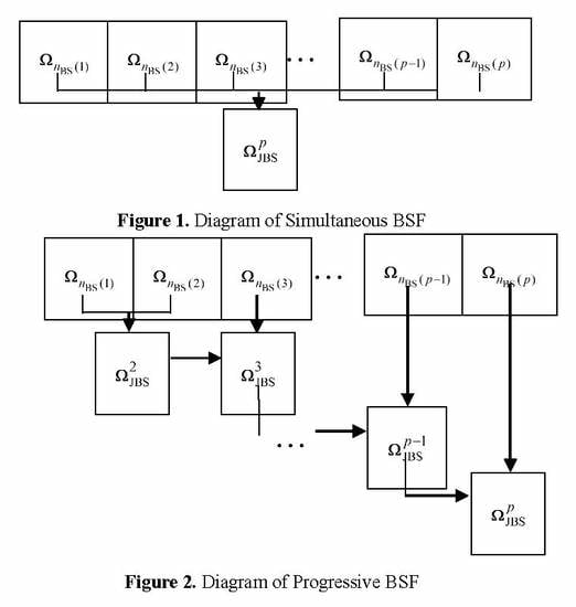
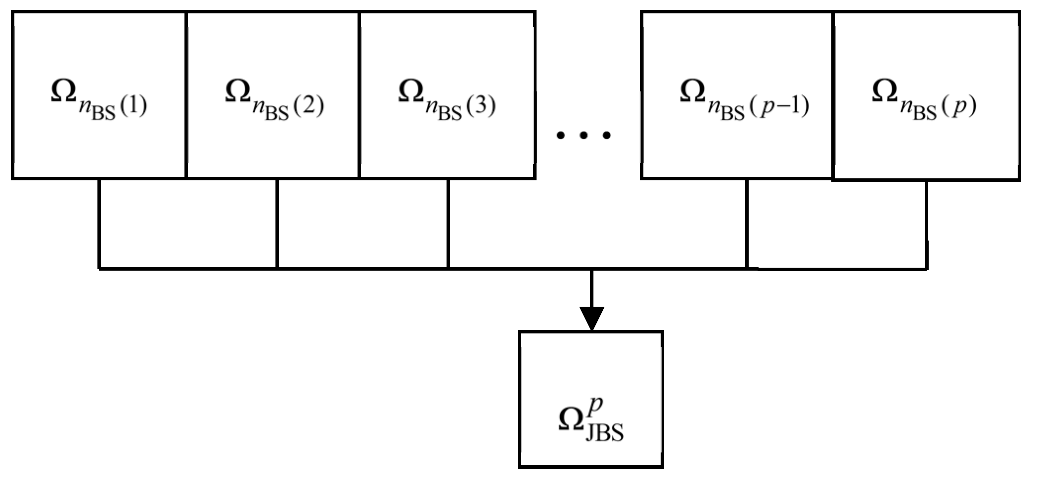
The first BSF method is to fuse all band subsets, , produced by p BS methods.
| Simultaneous Band Selection Fusion (SBSF) |
|
Figure 1 describes a diagram of fusing p band subsets, simultaneously, denoted by where BSj produces the band subset .
2.2. Progressive Band Selection Fusion
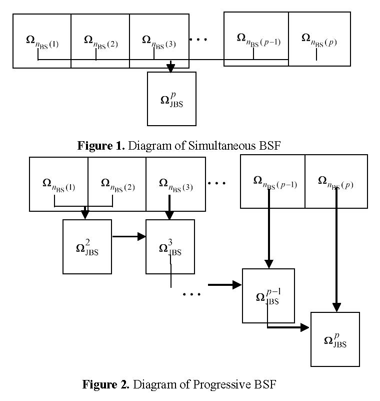
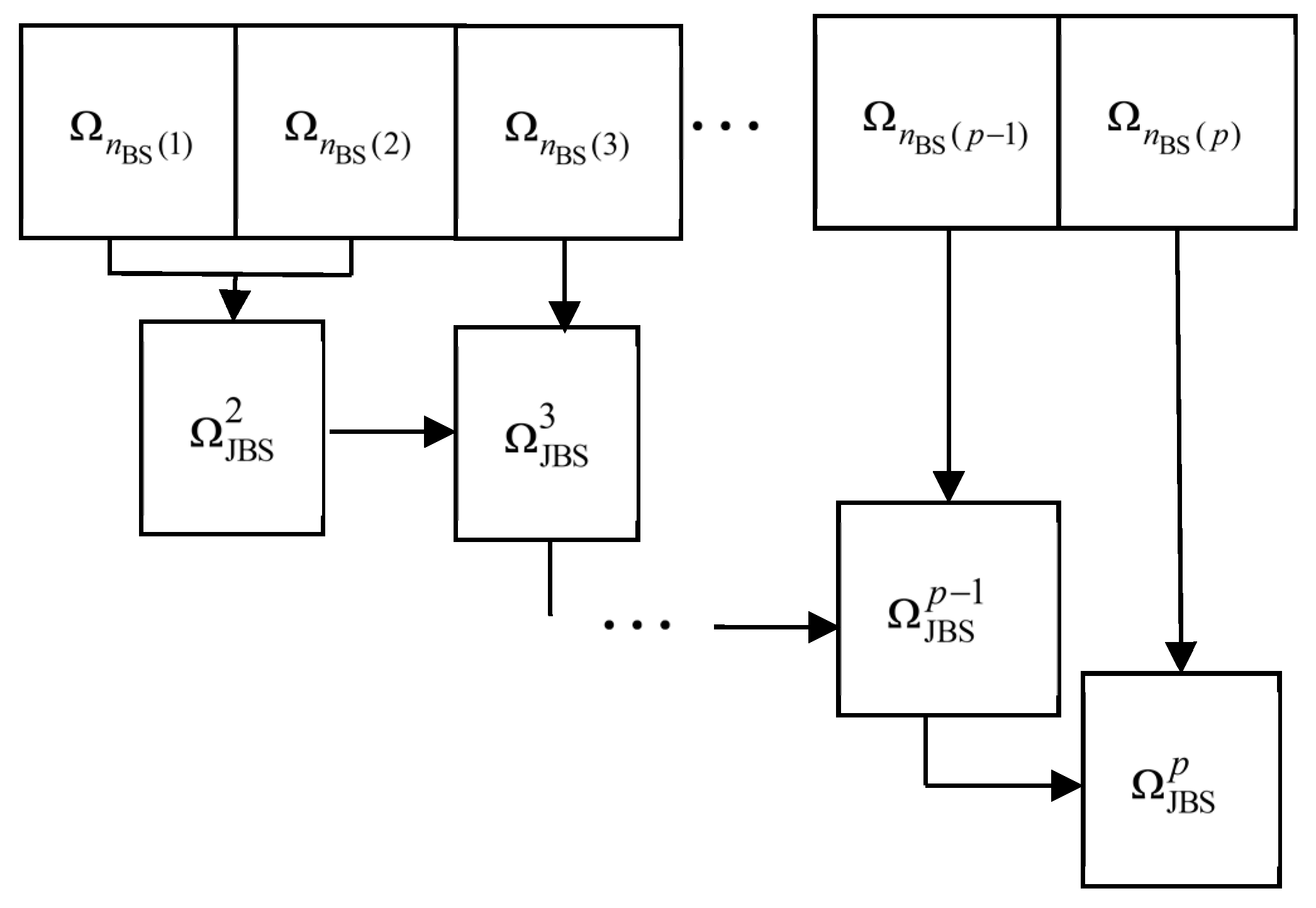
A second BSF method expands SBSF in multiple stages in a progressive manner, where each stage essentially performs two-band subsets fusion by SBSF.
| Progressive Band Selection Fusion (PBSF) |
|
Figure 2 depicts a diagram of how to implement PBSF progressively, denoted by , where BSj produces the band subset .
It is worth noting that the above PBSF can be also implemented in a more general fashion. It does not have to fuse two band subsets at a time, but rather small varying numbers, for example, three band subsets in the first stage, then four band subsets in the second stage.
Once the number of bands is determined for BS, such as virtual dimensionality (VD) or , we can select nBS bands from according to (5). There is a key difference between SBSF and PBSF. That is, SBSF waits for the final generated to select nBS bands, while PBSF selects nBS bands from after each fusion.
One major issue arising in the selection of prioritized bands is that once a band with high priority is selected, its adjacent bands may be also selected due to their close inter-band correlation with the selected band. With the use of BSF, this issue can be resolved, because bands are selected according to their frequencies appearing in different sets of band subsets, not the priority orders.
3. Real Hyperspectral Image Experiments
In this section, two applications are studied to demonstrate the utility of fusing various BSF methods using real hyperspectral images.
3.1. Linear Spectral Unmixing
HYDICE data was first used for linear spectral unmixing. Detailed information of HYDICE data is described in Appendix A.1.
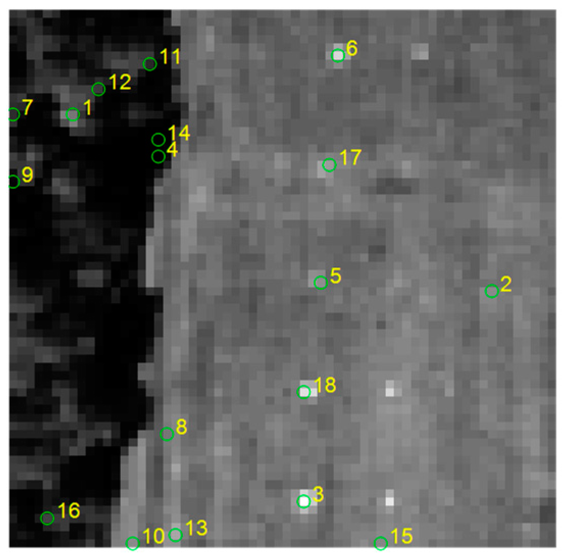
The virtual dimensionality (VD) of this scene was estimated by the Harsanyi–Farrand–Chang (HFC) method in [21,22,23] as 9. However, according to [24,25], nBS = 9 seemed insufficient, because when the automatic target generation process (ATGP) developed in [26] was used to find target pixels, only three panel pixels could be found among nine ATGP-found target pixels. In order for ATGP to find five panel pixels with each panel pixel corresponding to one individual row, it requires 18 pixels to do so, as shown in Figure 3.
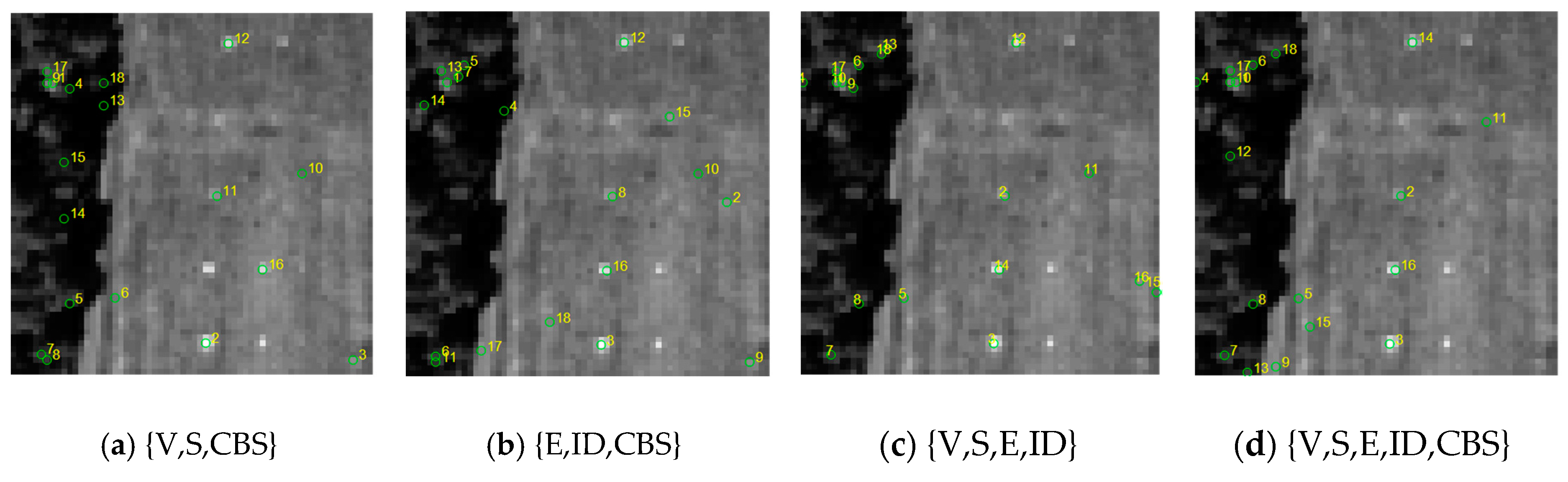
It should be noted that ATGP has been shown in [27] to be essentially the same as vertex component analysis (VCA) [28] and simplex growing algorithm (SGA) [29], as long as their initial conditions are chosen to be the same. Accordingly, ATGP can be used for the general purposes of target detection and endmember finding. So, in the following experiments, the value of VD, nVD used for BS was set to nBS = 18 [30,31]. Over the past years, many BS methods were developed [1,2,3,4,5,6,7,8,9,10,11,12,13,14,15,16,17,18,19,20]. It is impossible to cover all such methods. Instead, we have selected some representatives for our experiments, for example, second order statistics-based BP criteria: variance, constrained band selection (CBS), signal-to-noise ratio (SNR), and high order statistics BP criteria: entropy (E), information divergence (ID). SBSF and PBSF were then used to fuse these BS methods. Table 1 lists 18 bands selected by 6 individual band selection algorithms. Table 2 and Table 3 list 18 bands selected by various SBSF and PBSF methods. Figure 4, Figure 5 and Figure 6 show 18 target pixels found by ATGP using the 18 bands selected in Table 1, Table 2 and Table 3. Table 4 lists red panel pixels (in Figure A1b) found by ATGP in Figure 4, Figure 5 and Figure 6, where ATGP using only 18 bands selected by S, UBS, and E-ID-CBS (PBSF) could find panel pixels in each of the five different rows. The last column in Table 4 shows whether all the five categories of targets (red panels in Figure A1b) were found using p = 18; if yes, this column would give the order and the exact endmember where the last pixel was found as the fifth red panel pixel in Figure A1b.
Next, we used the 18 ATGP-found target pixels in Figure 4, Figure 5 and Figure 6 as image endmembers for fully constrained least squares (FCLS) developed in [32] to perform linear spectral unmixing. Table 5 tabulates their total FCLS-unmixed errors. For comparison, we also included the results using full bands and 18 bands selected by uniform band selection (UBS) in Table 2, where the smallest unmixed errors produced by the BS and BSF methods are boldfaced.
As we can see from Table 2, including five pure panel pixels found by S, UBS, and E-ID-CBS (PBSF) did not necessarily produce the best unmixing results. As a matter of fact, the best results were from FCLS using the bands selected by ID, which produced the smallest unmixed errors. These experiments demonstrated that in order for linear spectral unmixing to perform effectively, finding endmembers is not critical, but rather finding appropriate target pixels is more important and crucial. This was also confirmed in [33]. On the other hand, using bands selected by S and CBS also performed better than using the full band for spectral unmixing. Interestingly, if we further used BSF methods, then the FCLS-unmixed errors produced by bands selected by PBSF-based methods were smaller than that produced by using full bands and single BP criteria except ID.
3.2. Hyperspectral Image Classification
Three popular hyperspectral images, which have been studied extensively for hyperspectral image classification, were used for experiments—AVIRIS Purdue data, AVIRIS Salinas data, and ROSIS University of Pavia data. Detailed descriptions of these three images can be found in Appendix A.
According to recent work [1,34,35,36,37,38], the VD estimated for the three hyperspectral images were nVD = 18 for the Purdue data, nVD = 21 for Salinas, and nVD = 14 for the University of Pavia, as tabulated in Table 6, in which case nBS was determined by the false alarm probability (PF) 10−4.
Then, uniform band selection (UBS), variance (V), SNR (S), entropy (E), ID, CBS, and the proposed SBSF and PBSF were implemented to find the desired bands listed in Table 7.
Once the bands were selected in Table 7, two types of classification techniques were implemented for performance evaluation. One was a commonly used edge preserving filtering (EPF)-based spectral–spatial approach developed in [39]. In this EPF-based approach, four algorithms, EPF-B-c, EPF-G-c, EPF-B-g, and EPF-G-g, were shown to be best classification techniques, where “B” and “G” are used to specify bilateral filter and guided filter respectively, and “g” and “c” indicate that the first principal component and color composite of three principal components were used as reference images. Therefore, in the following experiments, the performance of various BSF techniques will be evaluated and compared to these four EPF-based techniques because of two main reasons. One is that these four techniques are available on websites and we could re-implement them for comparison. Another is that these four techniques were compared to other existing spectral–spatial classification methods in [39] to show their superiority.
While EPF-based methods are pure pixel-based classification techniques, the other type of classification technique is a subpixel detection-based method which was recently developed in [40], called iterative CEM (ICEM). In order to make fair comparison, ICEM was modified without nonlinear expansion. In addition, the ICEM implemented here is a little different from the ICEM with band selection nonlinear expansion (BSNE) in [40], in the sense that the ground truth was used to update new image cubes instead of the ICEM with BSNE in [40], which used classified results to update new image cubes. As a consequence, the ICEM results presented in this paper were better than ICEM with BSNE.
There are many parameters to compare the performance of different classification algorithms, among which POA, PAA, and PPR are very popular ones to show how a specific classification algorithm performs. POA is the overall accuracy probability, which is the total number of the correctly classified samples divided by the total number of test samples. PAA is the average accuracy probability, which is the mean of the percentage of correctly classified samples for each class. PPR is the precision rate probability by extending binary classification to a multi-class classification problem in terms of a multiple hypotheses testing formulation. Please refer to [40] for a detailed description of the three parameters.
Table 8 calculates POA, PAA, and PPR for Purdue’s Indian Pines produced by EPF-B-c, EPF-G-c, EPF-B-g, and EPF-G-g using full bands and bands selected in Table 7, and the same experiment’s results for the Salinas and University of Pavia data can be found in Table A1 and Table A2 in Appendix B, where EPF-methods could not be improved by BS in classification. This is mainly due to their use of principal components which contain full band information compared to BS methods, which only retain selected band information. It is also very interesting to note that compared to experiments conducted for spectral unmixing in Section 3.1, where ID was shown to be the best BS method, ID was the worst BS for all four EPF-B-c, EPF-G-c, EPF-B-g, and EPF-G-g methods. More importantly, whenever the BSF (both PBSF and SBSF) included ID as one of BS methods, the classification results were also the worst. These experiments demonstrated that ID was not suitable to be used for classification. Furthermore, experiments also showed that one BS method which is effective for one application may not be necessarily effective for another application.
In contrast to EPF-based methods which could not be improved by BS, ICEM coupled with BS behaved completely differently. Table 9 calculates POA, PAA, PPR, and the number of iterations for Purdue’s Indian Pines produced by ICEM using full bands and bands selected in Table 7, and the same experiment’s results for the Salinas and University of Pavia data can be found in Table A3 and Table A4 in Appendix B, where the best results are boldfaced. Apparently, all the POA and PAA results produced by ICEM in Table 9 and Table A3 and Table A4 in Appendix B were much better than those produced by EPF-based methods in Table 8 and Table A1 and Table A2, but the PPR results were reversed. Most interestingly, ID, which performed poorly for EPF-based methods for the three image scenes, now worked very effectively for ICEM using BS for the same three image scenes, specifically using BSF methods, which included ID as one of BS methods to be fused. Compared to the results using full bands, all BS and BSF methods performed better for both Purdue’s data and University of Pavia and slightly worse than using full bands for Salinas. Also, the experimental results showed that the three image scenes did have different image characteristics when ICEM was used as a classifier with bands selected by various BS and BSF methods. For example, for the Purdue data, all the BS and BSF methods did improve classification results in POA and PAA but not in PPR. This was not true for Salinas, where the best results were still produced by using full bands. For the University of Pavia, the results were right in between. That is, ICEM using full bands generally performed better than its using bands selected by single BS methods but worse than its using bands selected by BSF methods.
4. Discussions
Several interesting discussions are worthy of being mentioned.
The proposed BSF does not actually solve band de-correlation problem but rather mitigates the problem. Nevertheless, whether BSF is effective or not is indeed determined by how effective the BS algorithms used to be fused are. BS algorithms use band prioritization (BP) to rank all bands according to their priority scores calculated by a BP criterion selected by user’s preference. In this case, band de-correlation is generally needed to remove potentially redundant adjacent bands. If the selected BS algorithm is not appropriate and does not work effectively, how we can avoid this dilemma? So, a better way is to fuse two or more different BS algorithms to alleviate this problem. Our proposed BSF tries to address this exact issue. In other words, BSF can alleviate this but cannot fix this issue. Nevertheless, the more BP-based algorithms are fused, the less band correlation occurs. This can be seen from our experimental results. When two BP-based algorithms are fused, the bands selected by BSF are alternating. When more BP-based algorithms are fused, the BSF begins to select bands among different band subsets. This fact indicates that BSF tries to resolve the issue of band correlation as more BS algorithms are fused.
Since variance and SNR are second order statistics-based BP criteria, we may expect that their selected bands will be similar. Interestingly, this is not true according to Table 7. For the Purdue data, variance and SNR selected pretty much the same bands in their first five bands and then departed widely, with variance focusing on the rest of bands in the blue visible range, compared to SNR selecting most bands in red and near infrared ranges. However, for Salinas, both variance and SNR selected pretty much same or similar bands in the blue and green visible range. On the contrary, variance and SNR selected bands in a very narrow green visible range but completely disjointed band subsets for University of Pavia. As for CBS, it selected almost red and infrared ranges for both the Purdue and Salinas scenes, but all bands in the red visible range for University of Pavia. Now, if these three BS algorithms were fused by PBSF, it turned out that half of the selected bands were in the blue visible range and the other were in red/infrared range for the Purdue data and Salinas. By contrast, PBSF selected most bands in the blue and red/infrared ranges. On the other hand, if these variance, SNR, and CBS were fused by SBSF, the selected bands were split evenly in the blue and red/infrared ranges for the Purdue data, but most bands in the blue and green ranges, except for four bands in the red and infrared ranges for Salinas, and most bands in the blue range for University of Pavia, with four adjacent bands, 80–91, selected in the green range. According to Table 8, the best results were obtained by bands selected by SBSF across the board. Similar observations can be also made based on the fusion of entropy, ID, and CBS.
Whether or not a BS method is effective is completely determined by applications, which has been proven in this paper, especially when we compare the BS and BSF results for spectral unmixing and classification, which show that the most useful or sensitive BS methods are different.
The number of bands, nBS, to be selected also has a significant impact on the results. The nBS used in the experiments was selected based on VD, which is completely determined by image data characteristics, regardless of applications. It is our belief that in order for BS to perform effectively, the value of nBS should be custom-determined by a specific application.
It is known that there are two types of BS generally used for hyperspectral imaging. One is band prioritization (BP), which ranks all bands according to their priority scores calculated by a selected BP criterion. The other is search-based BS algorithms, according to a particularly designed band search strategy to solve a band optimization problem. This paper only focused on the first type of BS algorithms to illustrate the utility of BSF. Nevertheless, our proposed BSF can be also applicable to search-based BS algorithms. In this case, there was no need for band de-correlation. Since the experimental results are similar, their results were not included in this paper due to the limited space.
5. Conclusions
In general, a BS method is developed for a particular purpose. So, different BS methods produce different band subsets. Consequently, when a BS method is developed for one application, it may not work for another. It is highly desirable to fuse different BS methods designed for various applications so that the fused band set can not only work for one application but also for other applications. The BSF presented in this paper fits this need. It developed different strategies to fuse a number of BS methods. In particular, two versions of BSF were derived, simultaneous BSF (SBSF) and progressive BSF (PBSF). The main idea of BSF is to fuse bands by prioritizing fused bands according to their frequencies appearing in different band subsets. As a result, the fused band subset is more robust to various applications than a band subset produced by a single BS method. Additionally, such a fused band subset generally takes care of the band de-correlation issue. Several contributions are worth noting. First and foremost is the idea of BSF, which has never been explored in the past. Second, the fusion of different BS methods with different numbers of bands to be selected allows users to select the most effective and significant bands among different band subsets produced by different BS methods. Third, since fused bands are selected from different band subsets, their band correlation is largely reduced to avoid high inter-band correlation. Fourth, one bad band selected by a BS method will not have much effect on BSF performance because it may be filtered out by fusion. Finally, and most importantly, bands can be fused according to practical applications, simultaneously or progressively. For example, PBSF has potential in future hyperspectral data exploitation space communication, in which case BSF can take place during hyperspectral data transmission [33].
Author Contributions
Conceptualization, L.W. and Y.W.; Methodology, C.-I.C., L.W. and Y.W.; Experiments: Y.W.; Data analysis Y.W.; Writing—Original Draft Preparation, C.-I.C., and Y.W.; Writing—Revision: H.X. and Y.W.; Supervision, C.-I.C.
Funding
The work of Y.W. was supported in part by the National Nature Science Foundation of China (61801075), the Fundamental Research Funds for the Central Universities (3132019218, 3132019341), and Open Research Funds of State Key Laboratory of Integrated Services Networks (Xidian University). The work of L.W. is supported by the 111 Project (B17035). The work of C.-I.C. was supported by the Fundamental Research Funds for the Central Universities (3132019341).
Conflicts of Interest
The authors declare no conflict of interest.
Acronyms
| BS | Band Selection |
| BSF | Band Selection Fusion |
| BP | Band Prioritization |
| PBSF | Progressive BSF |
| SBSF | Simultaneous BSF |
| JBS | Joint Band Subset |
| VD | Virtual Dimensionality |
| E | Entropy |
| V | Variance |
| SNR (S) | Signal-to-Noise Ratio |
| ID | Information Divergence |
| CBS | Constrained Band Selection |
| UBS | Uniform Band Selection |
| HFC | Harsanyi–Farrand–Chang |
| NWHFC | Noise-Whitened HFC |
| ATGP | Automated Target Generation Process |
| OA | Overall Accuracy |
| AA | Average Accuracy |
| PR | Precision Rate |
Appendix A. Descriptions of Four Hyperspectral Data Sets
Four hyperspectral data sets were used in this paper. The first one, used for linear spectral unmixing, was acquired by the airborne hyperspectral digital imagery collection experiment (HYDICE) sensor, and the other three popular hyperspectral images available on the website http://www.ehu.eus/ccwintco/index.php?title=Hyperspectral_Remote_Sensing_Scenes, which have been studied extensively for hyperspectral image classification, were used for experiments.
Appendix A.1. HYDICE Data
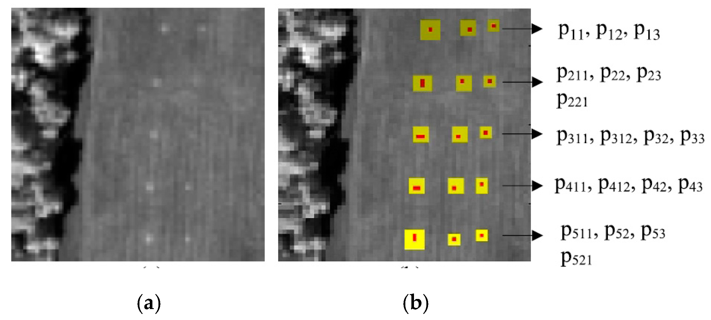
The image scene shown in Figure A1 was acquired by the airborne hyperspectral digital imagery collection experiment (HYDICE) sensor in August 1995 from a flight altitude of 10,000 ft. This scene has been studied extensively by many reports, such as [1,21]. There are 15 square panels with three different sizes, 3 × 3 m, 2 × 2 m, and 1 × 1 m, with its ground truth shown in Figure A1b, where the center and boundary pixels of objects are highlighted by red and yellow, respectively.
Figure A1.
(a) A hyperspectral digital imagery collection (HYDICE) panel scene which contains 15 panels; (b) ground truth map of the spatial locations of the 15 panels.
Figure A1.
(a) A hyperspectral digital imagery collection (HYDICE) panel scene which contains 15 panels; (b) ground truth map of the spatial locations of the 15 panels.

In particular, R (red color) panel pixels are denoted by pij, with rows indexed by and columns indexed by , except the panels in the first column with the second, third, fourth, and fifth rows, which are two-pixel panels, denoted by p211, p221, p311, p312, p411, p412, p511, p521. The 1.56 m-spatial resolution of the image scene suggests that most of the 15 panels are one pixel in size. As a result, there are a total of 19 R panel pixels. Figure A1b shows the precise spatial locations of these 19 R panel pixels, where red pixels (R pixels) are the panel center pixels and the pixels in yellow (Y pixels) are panel pixels mixed with the background.
Appendix A.2. AVIRIS Purdue Data
The second hyperspectral data set was a well-known airborne visible/infrared imaging spectrometer (AVIRIS) image scene, Purdue Indiana Indian Pines test site, shown in Figure A2a with its ground truth of 16 class maps in Figure A2b. It has a size of 145 × 145 × 220 pixel vectors, including water absorption bands (bands 104–108 and 150–163, 220).
Figure A2.
Purdue’s Indiana Indian Pines scene.

Appendix A.3. AVIRIS Salinas Data
The third hyperspectral data set was the Salinas scene, shown in Figure A3a, which was also captured by the AVIRIS sensor over Salinas Valley, California, and with a spatial resolution of 3.7 m per pixel and a spectral resolution of 10 nm. It has a size of 512 × 227 × 224, including 20 water absorption bands, 108–112, 154–167, and 224. Figure A3b,c shows the color composite of the Salinas image along with the corresponding ground truth class labels.
Figure A3.
Ground-truth of Salinas scene with 16 classes.

Appendix A.4. ROSIS Data
The last hyperspectral data set used for experiments was the University of Pavia, image shown in Figure A4, which is an urban area surrounding the University of Pavia, Italy. It was recorded by the ROSIS-03 satellite sensor. It has a size of 610 × 340 × 115 with a spatial resolution of 1.3 m per pixel and a spectral coverage ranging from 0.43 to 0.86 μm, with a spectral resolution of 4 nm (the 12 most noisy channels were removed before experiments). Nine classes of interest plus background class, class 0, were considered for this image.
Figure A4.
Ground-truth of the University of Pavia scene with nine classes.

Appendix B. Classification Results of Salinas and University of Pavia Data Sets

Table A1.
POA, PAA, PPR for Salinas, produced by EPF-B-c, EPF-G-c, EPF-B-g, and EPF-G-g using full bands and bands selected in Table 7.
Table A1.
POA, PAA, PPR for Salinas, produced by EPF-B-c, EPF-G-c, EPF-B-g, and EPF-G-g using full bands and bands selected in Table 7.
| BS and BSF Methods | EPF-B-c | EPF-G-c | EPF-B-g | EPF-G-g | ||||||||
|---|---|---|---|---|---|---|---|---|---|---|---|---|
| POA | PAA | PPR | POA | PAA | PPR | POA | PAA | PPR | POA | PAA | PPR | |
| Full bands | 0.9584 | 0.9829 | 0.9773 | 0.9679 | 0.9875 | 0.9826 | 0.9603 | 0.9840 | 0.9784 | 0.9616 | 0.9844 | 0.9789 |
| V | 0.9239 | 0.9665 | 0.9588 | 0.9257 | 0.9660 | 0.9613 | 0.9252 | 0.9667 | 0.9591 | 0.9180 | 0.9627 | 0.9557 |
| S | 0.9328 | 0.9687 | 0.9516 | 0.9351 | 0.9692 | 0.9556 | 0.9342 | 0.9696 | 0.9531 | 0.9280 | 0.9648 | 0.9475 |
| E | 0.9322 | 0.9707 | 0.9570 | 0.9358 | 0.9711 | 0.9605 | 0.9336 | 0.9710 | 0.9570 | 0.9250 | 0.9667 | 0.9530 |
| ID | 0.8236 | 0.8817 | 0.8682 | 0.8406 | 0.8979 | 0.8892 | 0.8245 | 0.8838 | 0.8697 | 0.8304 | 0.8884 | 0.8767 |
| CBS | 0.8593 | 0.9402 | 0.9337 | 0.8660 | 0.9483 | 0.9419 | 0.8604 | 0.9416 | 0.9353 | 0.8632 | 0.9442 | 0.9372 |
| UBS | 0.9558 | 0.9804 | 0.9754 | 0.9660 | 0.9857 | 0.9812 | 0.9583 | 0.9816 | 0.9765 | 0.9601 | 0.9826 | 0.9776 |
| V-S-CBS (PBSF) | 0.9039 | 0.9372 | 0.9403 | 0.9208 | 0.9469 | 0.9506 | 0.9071 | 0.9388 | 0.9420 | 0.9102 | 0.9407 | 0.9437 |
| E-ID-CBS (PBSF) | 0.9332 | 0.9693 | 0.9610 | 0.9490 | 0.9775 | 0.9733 | 0.9366 | 0.9709 | 0.9634 | 0.9407 | 0.9733 | 0.9668 |
| V-S-E-ID (PBSF) | 0.9342 | 0.9610 | 0.9513 | 0.9466 | 0.9766 | 0.9640 | 0.9360 | 0.9706 | 0.9530 | 0.9389 | 0.9721 | 0.9552 |
| V-S-E-ID-CBS (PBSF) | 0.9146 | 0.9448 | 0.9457 | 0.9301 | 0.9555 | 0.9582 | 0.9186 | 0.9473 | 0.9484 | 0.9218 | 0.9496 | 0.9511 |
| {V,S,CBS} (SBSF) | 0.9477 | 0.9775 | 0.9731 | 0.9590 | 0.9836 | 0.9806 | 0.9496 | 0.9784 | 0.9744 | 0.9523 | 0.9799 | 0.9760 |
| {E,ID,CBS} (SBSF) | 0.9220 | 0.9609 | 0.9585 | 0.9380 | 0.9717 | 0.9692 | 0.9261 | 0.9636 | 0.9610 | 0.9291 | 0.9656 | 0.9631 |
| {V,S,E,ID} (SBSF) | 0.9337 | 0.9675 | 0.9516 | 0.9448 | 0.9741 | 0.9641 | 0.9357 | 0.9681 | 0.9531 | 0.9359 | 0.9680 | 0.9537 |
| {V,S,E,ID,CBS} (SBSF) | 0.9227 | 0.9647 | 0.9476 | 0.9436 | 0.9751 | 0.9621 | 0.9259 | 0.9666 | 0.9501 | 0.9309 | 0.9689 | 0.9532 |
Table A2.
POA, PAA, and PPR for University of Pavia produced by EPF-B-c, EPF-G-c, EPF-B-g, and EPF-G-g using full bands and bands selected in Table 7.
Table A2.
POA, PAA, and PPR for University of Pavia produced by EPF-B-c, EPF-G-c, EPF-B-g, and EPF-G-g using full bands and bands selected in Table 7.
| BS and BSF Methods | EPF-B-c | EPF-G-c | EPF-B-g | EPF-G-g | ||||||||
|---|---|---|---|---|---|---|---|---|---|---|---|---|
| POA | PAA | PPR | POA | PAA | PPR | POA | PAA | PPR | POA | PAA | PPR | |
| Full bands | 0.9862 | 0.9848 | 0.9818 | 0.9894 | 0.9901 | 0.9863 | 0.9866 | 0.9852 | 0.9829 | 0.9853 | 0.9837 | 0.9820 |
| V | 0.9055 | 0.9332 | 0.8676 | 0.9139 | 0.9408 | 0.8776 | 0.9055 | 0.9344 | 0.8672 | 0.9067 | 0.9365 | 0.8697 |
| S | 0.8852 | 0.9205 | 0.8487 | 0.8910 | 0.9222 | 0.8556 | 0.8852 | 0.9190 | 0.8487 | 0.8850 | 0.9197 | 0.8489 |
| E | 0.9055 | 0.9332 | 0.8676 | 0.9139 | 0.9408 | 0.8776 | 0.9055 | 0.9344 | 0.8672 | 0.9067 | 0.9365 | 0.8697 |
| ID | 0.6543 | 0.7688 | 0.6659 | 0.6657 | 0.7814 | 0.6707 | 0.6543 | 0.7695 | 0.6662 | 0.6523 | 0.7676 | 0.6593 |
| CBS | 0.7227 | 0.8507 | 0.7320 | 0.7402 | 0.8567 | 0.7398 | 0.7218 | 0.8488 | 0.7292 | 0.7177 | 0.8439 | 0.7226 |
| UBS | 0.9811 | 0.9829 | 0.9731 | 0.9859 | 0.9865 | 0.9808 | 0.9820 | 0.9833 | 0.9750 | 0.9806 | 0.9810 | 0.9735 |
| V-S-CBS (PBSF) | 0.9088 | 0.9482 | 0.8867 | 0.9245 | 0.9566 | 0.9017 | 0.9126 | 0.9497 | 0.8900 | 0.9109 | 0.9474 | 0.8888 |
| E-ID-CBS (PBSF) | 0.8831 | 0.9268 | 0.8537 | 0.8990 | 0.9375 | 0.8653 | 0.8838 | 0.9290 | 0.8531 | 0.8822 | 0.9277 | 0.8520 |
| V-S-E-ID (PBSF) | 0.8662 | 0.9301 | 0.8441 | 0.8757 | 0.9365 | 0.8499 | 0.8695 | 0.9318 | 0.8456 | 0.8628 | 0.9298 | 0.8412 |
| V-S-E-ID-CBS (PBSF) | 0.9178 | 0.9497 | 0.8947 | 0.9260 | 0.9567 | 0.9030 | 0.9186 | 0.9498 | 0.8954 | 0.9175 | 0.9472 | 0.8941 |
| {V,S,CBS} (SBSF) | 0.8848 | 0.9135 | 0.8481 | 0.9014 | 0.9256 | 0.8623 | 0.8880 | 0.9152 | 0.8505 | 0.8882 | 0.9138 | 0.8497 |
| {E,ID,CBS} (SBSF) | 0.8504 | 0.9101 | 0.8368 | 0.8615 | 0.9210 | 0.8488 | 0.8508 | 0.9092 | 0.8370 | 0.8517 | 0.9088 | 0.8391 |
| {V,S,E,ID} (SBSF) | 0.9055 | 0.9332 | 0.8676 | 0.9139 | 0.9408 | 0.8776 | 0.9055 | 0.9344 | 0.8672 | 0.9067 | 0.9365 | 0.8697 |
| {V,S,E,ID,CBS} (SBSF) | 0.9055 | 0.9332 | 0.8676 | 0.9139 | 0.9408 | 0.8776 | 0.9055 | 0.9344 | 0.8672 | 0.9067 | 0.9365 | 0.8697 |
Table A3.
POA, PAA, PPR and the number of iterations calculated by ICEM using full bands and bands selected in Table 7 for Salinas data.
Table A3.
POA, PAA, PPR and the number of iterations calculated by ICEM using full bands and bands selected in Table 7 for Salinas data.
| BS and BSF Methods | POA | PAA | PPR | Iteration Times |
|---|---|---|---|---|
| Full bands | 0.9697 | 0.9662 | 0.9446 | 13 |
| V | 0.9621 | 0.9587 | 0.9467 | 19 |
| S | 0.9622 | 0.9573 | 0.9392 | 19 |
| E | 0.9622 | 0.9584 | 0.9445 | 18 |
| ID | 0.9588 | 0.9569 | 0.9432 | 20 |
| CBS | 0.9608 | 0.9581 | 0.9382 | 17 |
| UBS | 0.9609 | 0.9609 | 0.9418 | 15 |
| V-S-CBS (PBSF) | 0.9595 | 0.9530 | 0.9331 | 17 |
| E-ID-CBS (PBSF) | 0.9640 | 0.9597 | 0.9417 | 19 |
| V-S-E-ID (PBSF) | 0.9595 | 0.9520 | 0.9330 | 17 |
| V-S- E-ID-CBS (PBSF) | 0.9601 | 0.9548 | 0.9385 | 17 |
| {V,S,CBS} (SBSF) | 0.9577 | .09525 | 0.9423 | 16 |
| {E,ID,CBS} (SBSF) | 0.9615 | 0.9601 | 0.9439 | 19 |
| {V,S,E,ID} (SBSF) | 0.9645 | 0.9570 | 0.9423 | 19 |
| {V,S,E,ID,CBS} (SBSF) | 0.9659 | 0.9603 | 0.9457 | 19 |
Table A4.
POA, PAA, PPR and the number of iterations calculated by ICEM using full bands and bands selected in Table 7 for the University of Pavia data.
Table A4.
POA, PAA, PPR and the number of iterations calculated by ICEM using full bands and bands selected in Table 7 for the University of Pavia data.
| BS and BSF Methods | POA | PAA | PPR | Iteration Times |
|---|---|---|---|---|
| Full bands | 0.8853 | 0.8868 | 0.6878 | 75 |
| V | 0.8764 | 0.8731 | 0.6898 | 77 |
| S | 0.8722 | 0.8736 | 0.6868 | 92 |
| E | 0.8763 | 0.8730 | 0.6898 | 77 |
| ID | 0.8690 | 0.8553 | 0.6870 | 100 |
| CBS | 0.8842 | 0.8844 | 0.6906 | 100 |
| UBS | 0.8836 | 0.8857 | 0.6876 | 82 |
| V-S-CBS (PBSF) | 0.8886 | 0.8817 | 0.6962 | 92 |
| E-ID-CBS (PBSF) | 0.8965 | 0.8881 | 0.7078 | 99 |
| V-S-E-ID (PBSF) | 0.8904 | 0.8783 | 0.6974 | 87 |
| V-S-E-ID-CBS (PBSF) | 0.8993 | 0.8893 | 0.6998 | 100 |
| {V,S,CBS} (SBSF) | 0.8900 | 0.8878 | 0.6966 | 99 |
| {E,ID,CBS} (SBSF) | 0.8917 | 0.8906 | 0.6816 | 84 |
| {V,S,E,ID} (SBSF) | 0.8764 | 0.8731 | 0.6898 | 77 |
| {V,S,E,ID,CBS} (SBSF) | 0.8764 | 0.8731 | 0.6898 | 77 |
References
- Chang, C.-I. Hyperspectral Data Processing: Signal Processing Algorithm Design and Analysis; Wiley: Hoboken, NJ, USA, 2013. [Google Scholar]
- Mausel, P.W.; Kramber, W.J.; Lee, J.K. Optimum band selection for supervised classification of multispectral data. Photogramm. Eng. Remote Sens. 1990, 56, 55–60. [Google Scholar]
- Conese, C.; Maselli, F. Selection of optimum bands from TM scenes through mutual information analysis. ISPRS J. Photogramm. Remote Sens. 1993, 48, 2–11. [Google Scholar] [CrossRef]
- Chang, C.-I.; Du, Q.; Sun, T.S.; Althouse, M.L.G. A joint band prioritization and band decorrelation approach to band selection for hyperspectral image classification. IEEE Trans. Geosci. Remote Sens. 1999, 37, 2631–2641. [Google Scholar] [CrossRef]
- Keshava, N. Distance metrics and band selection in hyperspectral processing with applications to material identification and spectral libraries. IEEE Trans. Geosci. Remote Sens. 2004, 42, 1552–1565. [Google Scholar] [CrossRef]
- Martínez-Usó, A.; Pla, F.; Sotoca, J.M.; García-Sevilla, P. Clustering-based hyperspectral band selection using information measures. IEEE Trans. Geosci. Remote Sens. 2007, 45, 4158–4171. [Google Scholar] [CrossRef]
- Zare, A.; Gader, P. Hyperspectral band selection and endmember detection using sparisty promoting priors. IEEE Geosci. Remote Sens. Lett. 2008, 5, 256–260. [Google Scholar] [CrossRef]
- Du, Q.; Yang, H. Similarity-based unsupervised band selection for hyperspectral image analysis. IEEE Geosci. Remote Sens. Lett. 2008, 5, 564–568. [Google Scholar] [CrossRef]
- Xia, W.; Wang, B.; Zhang, L. Band selection for hyperspectral imagery: A new approach based on complex networks. IEEE Geosci. Remote Sens. Lett. 2013, 10, 1229–1233. [Google Scholar] [CrossRef]
- Huang, R.; He, M. Band selection based feature weighting for classification of hyperspectral data. IEEE Geosci. Remote Sens. Lett. 2005, 2, 156–159. [Google Scholar] [CrossRef]
- Koonsanit, K.; Jaruskulchai, C.; Eiumnoh, A. Band selection for dimension reduction in hyper spectral image using integrated information gain and principal components analysis technique. Int. J. Mach. Learn. Comput. 2012, 2, 248–251. [Google Scholar] [CrossRef]
- Yang, H.; Su, Q.D.H.; Sheng, Y. An efficient method for supervised hyperspectral band selection. IEEE Geosci. Remote Sens. Lett. 2011, 8, 138–142. [Google Scholar] [CrossRef]
- Su, H.; Du, Q.; Chen, G.; Du, P. Optimized hyperspectral band selection using particle swam optimization. IEEE J. Sel. Top. Appl. Earth Obs. Remote Sens. 2014, 7, 2659–2670. [Google Scholar] [CrossRef]
- Su, H.; Yong, B.; Du, Q. Hyperspectral band selection using improved firefly algorithm. IEEE Geosci. Remote Sens. Lett. 2016, 13, 68–72. [Google Scholar] [CrossRef]
- Yuan, Y.; Zhu, G.; Wang, Q. Hyperspectral band selection using multitask sparisty pursuit. IEEE Trans. Geosci. Remote Sens. 2015, 53, 631–644. [Google Scholar] [CrossRef]
- Yuan, Y.; Zheng, X.; Lu, X. Discovering diverse subset for unsupervised hyperspectral band selection. IEEE Trans. Image Process. 2017, 26, 51–64. [Google Scholar] [CrossRef] [PubMed]
- Chen, P.; Jiao, L. Band selection for hyperspectral image classification with spatial-spectral regularized sparse graph. J. Appl. Remote Sens. 2017, 11, 1–8. [Google Scholar] [CrossRef]
- Geng, X.; Sun, K.; Ji, L. Band selection for target detection in hyperspectral imagery using sparse CEM. Remote Sens. Lett. 2014, 5, 1022–1031. [Google Scholar] [CrossRef]
- Chang, C.-I.; Wang, S. Constrained band selection for hyperspectral imagery. IEEE Trans. Geosci. Remote Sens. 2006, 44, 1575–1585. [Google Scholar] [CrossRef]
- Chang, C.-I.; Liu, K.-H. Progressive band selection for hyperspectral imagery. IEEE Trans. Geosci. Remote Sens. 2014, 52, 2002–2017. [Google Scholar] [CrossRef]
- Tschannerl, J.; Ren, J.; Yuen, P.; Sun, G.; Zhao, H.; Yang, Z.; Wang, Z.; Marshall, S. MIMR-DGSA: Unsupervised hyperspectral band selection based on information theory and a modified discrete gravitational search algorithm. Inf. Fusion 2019, 51, 189–200. [Google Scholar] [CrossRef] [Green Version]
- Zhu, G.; Huang, Y.; Li, S.; Tang, J.; Liang, D. Hyperspectral band selection via rank minimization. IEEE Geosci. Remote Sens. Lett. 2017, 14, 2320–2324. [Google Scholar] [CrossRef]
- Wei, X.; Zhu, W.; Liao, B.; Cai, L. Scalable One-Pass Self-Representation Learning for Hyperspectral Band Selection. IEEE Trans. Geosci. Remote Sens. 2019, 57, 4360–4374. [Google Scholar] [CrossRef]
- Chang, C.-I.; Du, Q. Estimation of number of spectrally distinct signal sources in hyperspectral imagery. IEEE Trans. Geosci. Remote Sens. 2004, 42, 608–619. [Google Scholar] [CrossRef]
- Chang, C.-I.; Jiao, X.; Du, Y.; Chen, H.M. Component-based unsupervised linear spectral mixture analysis for hyperspectral imagery. IEEE Trans. Geosci. Remote Sens. 2011, 49, 4123–4137. [Google Scholar] [CrossRef]
- Ren, H.; Chang, C.-I. Automatic spectral target recognition in hyperspectral imagery. IEEE Trans. Aerosp. Electron. Syst. 2003, 39, 1232–1249. [Google Scholar]
- Chang, C.-I.; Chen, S.Y.; Li, H.C.; Wen, C.-H. A comparative analysis among ATGP, VCA and SGA for finding endmembers in hyperspectral imagery. IEEE J. Sel. Top. Appl. Earth Obs. Remote Sens. 2016, 9, 4280–4306. [Google Scholar] [CrossRef]
- Nascimento, J.M.P.; Bioucas-Dias, J.M. Vertex component analysis: A fast algorithm to unmix hyperspectral data. IEEE Trans. Geosci. Remote Sens. 2005, 43, 898–910. [Google Scholar] [CrossRef]
- Chang, C.-I.; Wu, C.; Liu, W.; Ouyang, Y.C. A growing method for simplex-based endmember extraction algorithms. IEEE Trans. Geosci. Remote Sens. 2006, 44, 2804–2819. [Google Scholar] [CrossRef]
- Chang, C.-I.; Jiao, X.; Du, Y.; Chang, M.-L. A review of unsupervised hyperspectral target analysis. EURASIP J. Adv. Signal Process. 2010, 2010, 503752. [Google Scholar] [CrossRef]
- Li, F.; Zhang, P.P.; Lu, H.C.H. Unsupervised Band Selection of Hyperspectral Images via Multi-Dictionary Sparse Representation. IEEE Access 2018, 6, 71632–71643. [Google Scholar] [CrossRef]
- Heinz, D.; Chang, C.-I. Fully constrained least squares linear mixture analysis for material quantification in hyperspectral imagery. IEEE Trans. Geosci. Remote Sens. 2001, 39, 529–545. [Google Scholar] [CrossRef]
- Chang, C.-I. Real-Time Progressive Image Processing: Endmember Finding and Anomaly Detection; Springer: New York, NY, USA, 2016. [Google Scholar]
- Chang, C.-I. A unified theory for virtual dimensionality of hyperspectral imagery. In Proceedings of the High-Performance Computing in Remote Sensing Conference, SPIE 8539, Edinburgh, UK, 24–27 September 2012. [Google Scholar]
- Chang, C.-I. Real Time Recursive Hyperspectral Sample and Band Processing; Springer: New York, NY, USA, 2017. [Google Scholar]
- Chang, C.-I. Hyperspectral Imaging: Techniques for Spectral Detection and Classification; Kluwer Academic/Plenum Publishers: New York, NY, USA, 2003. [Google Scholar]
- Chang, C.-I. Spectral Inter-Band Discrimination Capacity of Hyperspectral Imagery. IEEE Trans. Geosci. Remote Sens. 2018, 56, 1749–1766. [Google Scholar] [CrossRef]
- Harsanyi, J.C.; Farrand, W.; Chang, C.-I. Detection of subpixel spectral signatures in hyperspectral image sequences. In Proceedings of the American Society of Photogrammetry & Remote Sensing Annual Meeting, Reno, NV, USA, 25–28 April 1994; pp. 236–247. [Google Scholar]
- Kang, X.; Li, S.; Benediktsson, J.A. Spectral-spatial hyperspectral image classification with edge-preserving filtering. IEEE Trans. Geosci. Remote Sens. 2014, 52, 2666–2677. [Google Scholar] [CrossRef]
- Xue, B.; Yu, C.; Wang, Y.; Song, M.; Li, S.; Wang, L.; Chen, H.M.; Chang, C.-I. A subpixel target approach to hyperpsectral image classification. IEEE Trans. Geosci. Remote Sens. 2017, 55, 5093–5114. [Google Scholar] [CrossRef]
Figure 1.
Diagram of simultaneous band selection fusion (BSF).

Figure 2.
Diagram of progressive BSF.

Figure 3.
The 18 target pixels found by automatic target generation process (ATGP).

Figure 4.
The 18 pixels found by automatic target generation process (ATGP) using the full bands and selected bands in Table 1.
Figure 4.
The 18 pixels found by automatic target generation process (ATGP) using the full bands and selected bands in Table 1.

Figure 5.
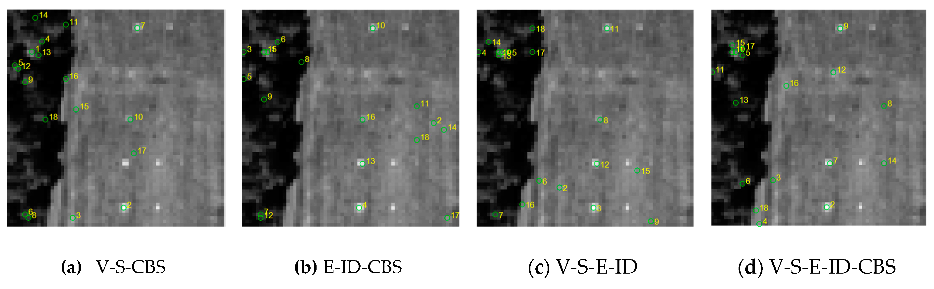
18 pixels found by ATGP using SBSF and the selected bands in Table 2.
Figure 5.
18 pixels found by ATGP using SBSF and the selected bands in Table 2.

Figure 6.
The 18 pixels found by ATGP using PBSF and the selected bands in Table 3.
Figure 6.
The 18 pixels found by ATGP using PBSF and the selected bands in Table 3.

Table 1.
The 18 bands selected by variance, signal-to-noise ratio (SNR), entropy, information divergence (ID), and constrained band selection (CBS).
Table 1.
The 18 bands selected by variance, signal-to-noise ratio (SNR), entropy, information divergence (ID), and constrained band selection (CBS).
| BS Methods | Selected Bands (p = 18) | |||||||||||||||||
|---|---|---|---|---|---|---|---|---|---|---|---|---|---|---|---|---|---|---|
| V | 60 | 61 | 67 | 66 | 65 | 59 | 57 | 68 | 62 | 64 | 56 | 78 | 77 | 76 | 79 | 63 | 53 | 80 |
| S | 78 | 80 | 93 | 91 | 92 | 95 | 89 | 94 | 90 | 88 | 102 | 96 | 79 | 82 | 105 | 62 | 107 | 108 |
| E | 65 | 60 | 67 | 53 | 66 | 61 | 52 | 68 | 59 | 64 | 62 | 78 | 77 | 57 | 79 | 49 | 76 | 56 |
| ID | 154 | 157 | 156 | 153 | 150 | 158 | 145 | 164 | 163 | 160 | 142 | 144 | 148 | 143 | 141 | 152 | 155 | 135 |
| CBS | 62 | 77 | 63 | 61 | 13 | 91 | 30 | 69 | 76 | 56 | 38 | 45 | 16 | 20 | 39 | 34 | 24 | 47 |
| UBS | 1 | 10 | 19 | 28 | 37 | 46 | 55 | 64 | 73 | 82 | 91 | 100 | 109 | 118 | 127 | 136 | 145 | 154 |
Table 2.
The 18 bands selected by various simultaneous band selection fusion (SBSF) methods.
| SBSF Methods | Fused Bands (p = 18) | |||||||||||||||||
|---|---|---|---|---|---|---|---|---|---|---|---|---|---|---|---|---|---|---|
| {V,S} | 78 | 80 | 62 | 79 | 60 | 61 | 67 | 93 | 66 | 91 | 65 | 92 | 59 | 95 | 57 | 89 | 68 | 94 |
| {E,ID} | 65 | 154 | 60 | 157 | 67 | 156 | 53 | 153 | 66 | 150 | 61 | 158 | 52 | 145 | 68 | 164 | 59 | 163 |
| {V,S,CBS} | 62 | 78 | 61 | 77 | 80 | 63 | 91 | 76 | 56 | 79 | 60 | 67 | 93 | 66 | 13 | 65 | 92 | 59 |
| {E,ID,CBS} | 62 | 77 | 61 | 76 | 56 | 65 | 154 | 60 | 157 | 63 | 67 | 156 | 53 | 153 | 13 | 66 | 150 | 91 |
| {V,S,E,ID} | 78 | 62 | 79 | 60 | 65 | 61 | 80 | 67 | 53 | 66 | 59 | 57 | 68 | 64 | 56 | 77 | 76 | 154 |
| {V,S,E,ID,CBS} | 62 | 78 | 61 | 77 | 76 | 56 | 79 | 60 | 65 | 80 | 63 | 67 | 53 | 66 | 91 | 59 | 57 | 68 |
Table 3.
The 18 bands selected by various progressive band selection fusion (PBSF) methods.
| PBSF Methods | Fused Bands (p = 18) | |||||||||||||||||
|---|---|---|---|---|---|---|---|---|---|---|---|---|---|---|---|---|---|---|
| V-S | 78 | 80 | 62 | 79 | 60 | 61 | 67 | 93 | 66 | 91 | 65 | 92 | 59 | 95 | 57 | 89 | 68 | 94 |
| E-ID | 65 | 154 | 60 | 157 | 67 | 156 | 53 | 153 | 66 | 150 | 61 | 158 | 52 | 145 | 68 | 164 | 59 | 163 |
| V-S-CBS | 62 | 78 | 61 | 77 | 80 | 63 | 91 | 76 | 56 | 79 | 60 | 67 | 93 | 66 | 13 | 65 | 92 | 59 |
| E-ID-CBS | 62 | 77 | 61 | 76 | 56 | 65 | 154 | 60 | 157 | 63 | 67 | 156 | 53 | 153 | 13 | 66 | 150 | 91 |
| V-S-E-ID | 62 | 65 | 60 | 67 | 78 | 66 | 61 | 53 | 80 | 154 | 52 | 93 | 68 | 91 | 59 | 157 | 64 | 92 |
| V-S-E-ID-CBS | 62 | 154 | 78 | 157 | 65 | 156 | 80 | 153 | 60 | 150 | 93 | 158 | 61 | 145 | 91 | 164 | 67 | 163 |
| Various BS and BSF Methods | p = 18 | p = 9 | Last Pixel Found as the Fifth R Panel Pixel Using p = 18 |
|---|---|---|---|
| Full bands | p11, p312, p411, p521 | p11, p312, p521 | no |
| V | p11, p312, p521 | p312, p521 | no |
| S | p11, p22, p311, p412, p521 | p11, p311, p521 | 16th pixel, p412 |
| E | p11, p311, p521 | p311, p521 | no |
| ID | p11, p211, p412, p521 | p11, p211, p412, p521 | no |
| CBS | p11, p312, p411, p521 | p312, p521 | no |
| UBS | p11, p211, p311, p412, p521 | p11, p311, p521 | 13th pixel, p412 |
| V-S-CBS (PBSF) | p11, p312, p42, p521 | P412, p521 | no |
| E-ID-CBS (PBSF) | p11, p22, p312, p412, p521 | p11, p412, p521 | 16th pixel, p412 |
| V-S-E-ID (PBSF) | p11, p312, p412, p521 | p521 | no |
| V-S- E-ID-CBS (PBSF) | p11, p312, p412, p521 | p11, p521, p53 | no |
| {V,S,CBS} (SBSF) | p11, p312, p521 | p412 | no |
| {E,ID,CBS} (SBSF) | p11, p311, p412, p521 | p22, p521 | no |
| {V,S,E,ID} (SBSF) | p11, p312, p412, p521 | p412, p521 | no |
| {V,S,E,ID,CBS} (SBSF) | p11, p211, p412, p521 | p11, p312, p521 | no |
Table 5.
Total fully constrained least squares (FCLS)-unmixed errors produced by using 18 target pixels in Table 4 and full bands, uniform band selection (UBS), Variance (V), signal-to-noise ratio (S), entropy (E), information divergence (ID), constrained band selection (CBS), and SBSF and PBSF fusion methods using bands selected in Table 2 and Table 3.
| BS Methods | Unmixed Error |
|---|---|
| Full bands | 222.09 |
| UBS | 245.58 |
| V | 268.71 |
| S | 211.27 |
| E | 296.72 |
| ID | 22.104 |
| CBS | 207.32 |
| V-S-CBS (PBSF) | 209.22 |
| E-ID-CBS (PBSF) | 195.27 |
| V-S-E-ID (PBSF) | 201.51 |
| V-S-E-ID-CBS (PBSF) | 96.203 |
| {V,S,CBS} (SBSF) | 181.70 |
| {E,ID,CBS} (SBSF) | 228.63 |
| {V,S,E,ID} (SBSF) | 263.62 |
| {V,S,E,ID,CBS} (SBSF) | 249.34 |
Table 6.
nBS estimated by HFC/NWHFC (Harsanyi–Farrand–Chang/Noise-whitened HFC).
| PF = 10−1 | PF = 10−2 | PF = 10−3 | PF = 10−4 | PF = 10−5 | |
|---|---|---|---|---|---|
| Purdue | 73/21 | 49/19 | 35/18 | 27/18 | 25/17 |
| Salinas | 32/33 | 28/24 | 25/21 | 21/21 | 20/20 |
| University of Pavia | 25/34 | 21/27 | 16/17 | 14/14 | 13/12 |
Table 7.
Bands selected by various BS methods and SBSF and PBSF.
| BS methods | Purdue Indian Pines (18 bands) | Salinas (21 bands) | University of Pavia (14 bands) |
|---|---|---|---|
| UBS | 1/13/25/37/49/61/73/85/97/109/ 121/133/145/157/169/181/193/205 | 1/11/21/31/41/51/61/71/81/91/ 101/111/121/131/141/151/161/ 171/181/191/201 | 1/8/15/22/29/36/43/ 50/57/64/71/78/85/92 |
| V | 29/28/27/26/25/30/42/32/41/24/33/ 23/31/43/22/44/39/21 | 45/46/42/47/44/48/52/51/53/41/ 54/55/50/56/49/57/43/58/40/32/34 | 91/88/90/89/87/92/ 93/95/94/96/82/86/ 83/97 |
| S | 28/27/26/29/30/123/121/122/25/ 120/124/119/24/129/131/127/130/125 | 46/45/74/52/55/71/72/56/53/73/ 54/76/75/57/48/70/50/77/44/51/47 | 63/62/64/61/65/60/ 59/66/67/58/68/69/ 48/57 |
| E | 41/42/43/44/39/29/28/48/49/25/51/ 50/52/27/45/31/24/38 | 42/47/46/45/44/51/41/55/53/52/ 48/54/56/49/50/57/35/40/58/36/37 | 91/90/88/92/89/87/ 95/93/94/96/82/83/ 86/97 |
| ID | 156/157/158/220/155/159/161/160/ 162/95/4/219/154/2/190/32/153/1 | 107/108/109/110/111/112/113/ 114/115/116/152/153/154/155/ 156/157/158/159/160/161/162 | 8/10/9/11/7/12/13/ 14/15/6/16/17/18/19 |
| CBS (LCMV-BCC) | 9/114/153/198/191/159/152/163/ 161/130/167/150/219/108/160/ 180/215/213 | 153/154/113/152/167/114/223/ 222/224/166/115/107/112/168/ 116/165/221/109/174/151/218 | 37/38/39/40/36/32/ 41/33/42/31/34/30/ 43/35 |
| V-S-CBS (PBSF) | 9/28/29/114/27/153/26/198/25/191/ 30/159/24/152/123/163/42/161 | 45/153/46/154/47/113/52/152/44/ 167/55/114/48/223/51/222/56/224/ 53/166/54 | 37/63/38/91/39/62/ 40/88/36/64/32/90/ 41/61 |
| E-ID-CBS (PBSF) | 153/159/161/9/156/41/157/42/158/ 114/220/43/155/44/160/198/39/162 | 42/107/47/153/46/154/45/109/44/ 113/51/152/41/112/55/114/53/115/ 52/116/48 | 8/91/37/90/10/88/38/ 92/9/89/39/87/11/95 |
| V-S-E-ID (PBSF) | 28/29/27/41/26/25/30/42/43/44/39/ 156/32/157/24/33/123/23 | 45/46/42/52/47/55/44/53/48/54/ 56/51/41/107/108/50/74/49/109/ 57/43 | 91/88/90/89/87/92/ 95/8/63/10/62/93/9/94 |
| V-S- E-ID-CBS (PBSF) | 28/156/29/157/27/158/26/220/30/ 155/25/159/24/161/41/160/42/162 | 113/107/112/109/45/153/47/154/ 46/44/152/51/167/52/114/55/223/ 53/222/48/224 | 37/91/38/90/39/88/8/ 40/36/63/10/32/41/92 |
| {V,S,CBS} (SBSF) | 28/29/27/26/25/30/24/130/9/114/ 153/198/191/123/159/42/121/152 | 45/46/47/52/44/55/48/51/56/53/ 54/50/57/153/154/42/74/113/152/ 167/71 | 37/63/91/38/62/88/ 39/64/90/40/61/89/ 36/65 |
| {E,ID,CBS} (SBSF) | 153/159/161/160/219/9/41/156/42/ 114/157/43/158/44/198/220/39/155 | 107/153/154/109/113/152/112/ 114/115/116/42/47/108/46/45/110/ 44/111/167/51/41 | 8/37/91/10/38/90/9/ 39/88/11/40/92/7/36 |
| {V,S,E,ID} (SBSF) | 28/29/27/25/24/41/42/26/43/44/30/ 39/32/31/156/157/158/220 | 45/46/47/52/44/55/48/51/56/53/54/ 50/57/42/41/49/40/58/107/108/74 | 91/88/90/89/92/87/ 93/95/94/96/82/83/ 86/97 |
| {V,S,E,ID,CBS} (SBSF) | 28/29/27/25/24/41/42/26/43/153/ 44/30/39/159/161/32/160/130 | 45/46/47/52/44/55/48/51/56/53/ 54/50/57/42/107/153/154/109/113/ 152/112 | 91/88/90/89/92/87/ 93/95/94/96/82/83/ 86/97 |
Table 8.
POA, PAA, PPR for Purdue’s Indian Pines produced by EPF-B-c, EPF-G-c, EPF-B-g and EPF-G-g using full bands and bands selected in Table 7.
Table 8.
POA, PAA, PPR for Purdue’s Indian Pines produced by EPF-B-c, EPF-G-c, EPF-B-g and EPF-G-g using full bands and bands selected in Table 7.
| BS and BSF Methods | EPF-B-c | EPF-G-c | EPF-B-g | EPF-G-g | ||||||||
|---|---|---|---|---|---|---|---|---|---|---|---|---|
| POA | PAA | PPR | POA | PAA | PPR | POA | PAA | PPR | POA | PAA | PPR | |
| Full bands | 0.8973 | 0.9282 | 0.9177 | 0.8896 | 0.9313 | 0.9186 | 0.8938 | 0.9269 | 0.9146 | 0.8932 | 0.9389 | 0.9121 |
| V | 0.8264 | 0.9011 | 0.8816 | 0.8297 | 0.9029 | 0.8805 | 0.8276 | 0.8938 | 0.8814 | 0.8255 | 0.9040 | 0.8782 |
| S | 0.8054 | 0.8161 | 0.7873 | 0.8096 | 0.8409 | 0.8573 | 0.8051 | 0.8126 | 0.7834 | 0.8000 | 0.8406 | 0.8223 |
| E | 0.8361 | 0.9062 | 0.8901 | 0.8296 | 0.9107 | 0.8826 | 0.8371 | 0.9027 | 0.8878 | 0.8352 | 0.9129 | 0.8859 |
| ID | 0.6525 | 0.5372 | 0.5232 | 0.6441 | 0.5289 | 0.5123 | 0.6532 | 0.5360 | 0.5282 | 0.6499 | 0.5360 | 0.5357 |
| CBS | 0.8119 | 0.8630 | 0.8630 | 0.8000 | 0.8010 | 0.8519 | 0.8116 | 0.8231 | 0.8628 | 0.8024 | 0.8407 | 0.8572 |
| V-S-CBS (PBSF) | 0.8336 | 0.8587 | 0.8687 | 0.8278 | 0.8255 | 0.8009 | 0.8363 | 0.8577 | 0.8698 | 0.8315 | 0.8526 | 0.8693 |
| E-ID-CBS (PBSF) | 0.7698 | 0.8091 | 0.7945 | 0.7473 | 0.7879 | 0.7728 | 0.7658 | 0.8076 | 0.7926 | 0.7650 | 0.8064 | 0.7949 |
| V-S-E-ID (PBSF) | 0.8315 | 0.9153 | 0.8836 | 0.8249 | 0.9078 | 0.8725 | 0.8321 | 0.9130 | 0.8830 | 0.8239 | 0.9045 | 0.8734 |
| V-S-E-ID-CBS (PBSF) | 0.6825 | 0.7197 | 0.7449 | 0.6623 | 0.6884 | 0.7266 | 0.6794 | 0.6865 | 0.7408 | 0.6791 | 0.7237 | 0.7403 |
| {V,S,CBS} (SBSF) | 0.8540 | 0.9036 | 0.8964 | 0.8529 | 0.8969 | 0.8942 | 0.8506 | 0.8881 | 0.8923 | 0.8531 | 0.9139 | 0.8935 |
| {E,ID,CBS} (SBSF) | 0.7793 | 0.7980 | 0.8099 | 0.7541 | 0.7733 | 0.7330 | 0.7710 | 0.7916 | 0.7991 | 0.7760 | 0.8059 | 0.8102 |
| {V,S,E,ID} (SBSF) | 0.7771 | 0.8484 | 0.8495 | 0.7704 | 0.8409 | 0.8247 | 0.7740 | 0.8491 | 0.8510 | 0.7761 | 0.8461 | 0.8441 |
| {V,S,E,ID,CBS} (SBSF) | 0.8300 | 0.8884 | 0.8677 | 0.8134 | 0.8680 | 0.8451 | 0.8279 | 0.8827 | 0.8483 | 0.8205 | 0.8814 | 0.8654 |
Table 9.
POA, PAA, PPR and the number of iterations calculated by ICEM using full bands and the bands selected in Table 7 for Purdue’s data.
Table 9.
POA, PAA, PPR and the number of iterations calculated by ICEM using full bands and the bands selected in Table 7 for Purdue’s data.
| BS and BSF Methods | POA | PAA | PPR | Iteration Times |
|---|---|---|---|---|
| Full bands | 0.9650 | 0.9673 | 0.9018 | 24 |
| V | 0.9715 | 0.9767 | 0.8909 | 30 |
| S | 0.9717 | 0.9750 | 0.8826 | 29 |
| E | 0.9700 | 0.9736 | 0.8940 | 30 |
| ID | 0.9728 | 0.9762 | 0.8940 | 31 |
| CBS | 0.9729 | 0.9791 | 0.8871 | 30 |
| UBS | 0.9699 | 0.9753 | 0.8852 | 29 |
| V-S-CBS (PBSF) | 0.9738 | 0.9745 | 0.8822 | 30 |
| E-ID-CBS (PBSF) | 0.9720 | 0.9760 | 0.8873 | 30 |
| V-S-E-ID (PBSF) | 0.9742 | 0.9773 | 0.8833 | 30 |
| V-S-E-ID-CBS (PBSF) | 0.9751 | 0.9760 | 0.8925 | 33 |
| {V,S,CBS} (SBSF) | 0.9701 | 0.9729 | 0.8781 | 27 |
| {E,ID,CBS} (SBSF) | 0.9737 | 0.9762 | 0.8912 | 31 |
| {V,S,E,ID} (SBSF) | 0.9723 | 0.9750 | 0.8953 | 31 |
| {V,S,E,ID,CBS} (SBSF) | 0.9701 | 0.9767 | 0.8867 | 31 |
© 2019 by the authors. Licensee MDPI, Basel, Switzerland. This article is an open access article distributed under the terms and conditions of the Creative Commons Attribution (CC BY) license (http://creativecommons.org/licenses/by/4.0/).
Share and Cite
MDPI and ACS Style
Wang, Y.; Wang, L.; Xie, H.; Chang, C.-I. Fusion of Various Band Selection Methods for Hyperspectral Imagery. Remote Sens. 2019, 11, 2125. https://doi.org/10.3390/rs11182125
AMA Style
Wang Y, Wang L, Xie H, Chang C-I. Fusion of Various Band Selection Methods for Hyperspectral Imagery. Remote Sensing. 2019; 11(18):2125. https://doi.org/10.3390/rs11182125
Chicago/Turabian StyleWang, Yulei, Lin Wang, Hongye Xie, and Chein-I Chang. 2019. "Fusion of Various Band Selection Methods for Hyperspectral Imagery" Remote Sensing 11, no. 18: 2125. https://doi.org/10.3390/rs11182125
Note that from the first issue of 2016, this journal uses article numbers instead of page numbers. See further details here.