Investigation of a Small Landslide in the Qinghai-Tibet Plateau by InSAR and Absolute Deformation Model

 , , ,
, , ,
Abstract
:
1. Introduction
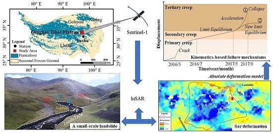
2. Study Area
3. Datasets and Processing
3.1. Digital Elevation Models (DEM) Producing
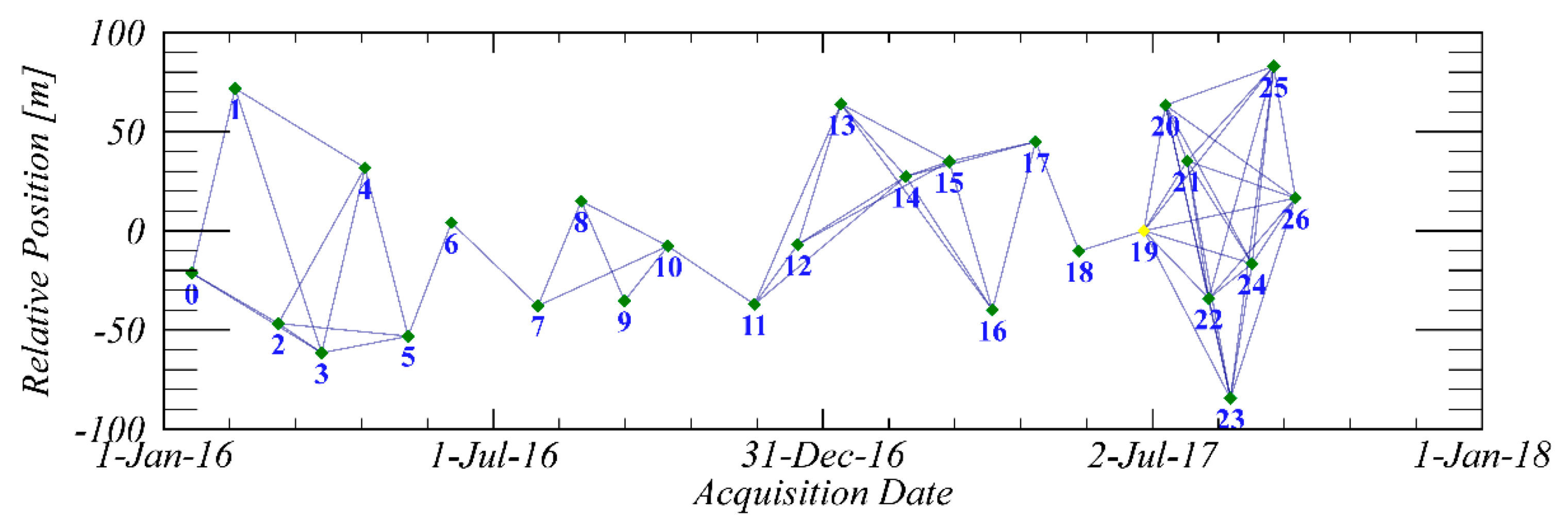
3.2. Short Baseline Interferometry
3.3. Calculation of Absolute Surface Displacements
3.4. Remote Sensing Images
3.5. Local Precipitation and Soil Sampling
4. Results
4.1. InSAR Landslides Analysis
4.2. Landslide Characteristics
4.3. Quantification of Absolute Surface Displacements
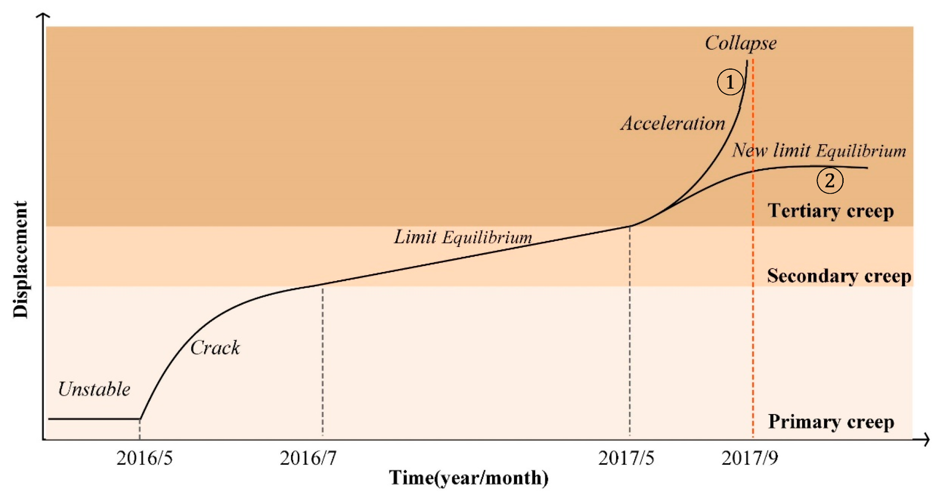
4.4. Interpreted Kinematics-based Failure Mechanism through the Satellite InSAR Data
5. Discussion
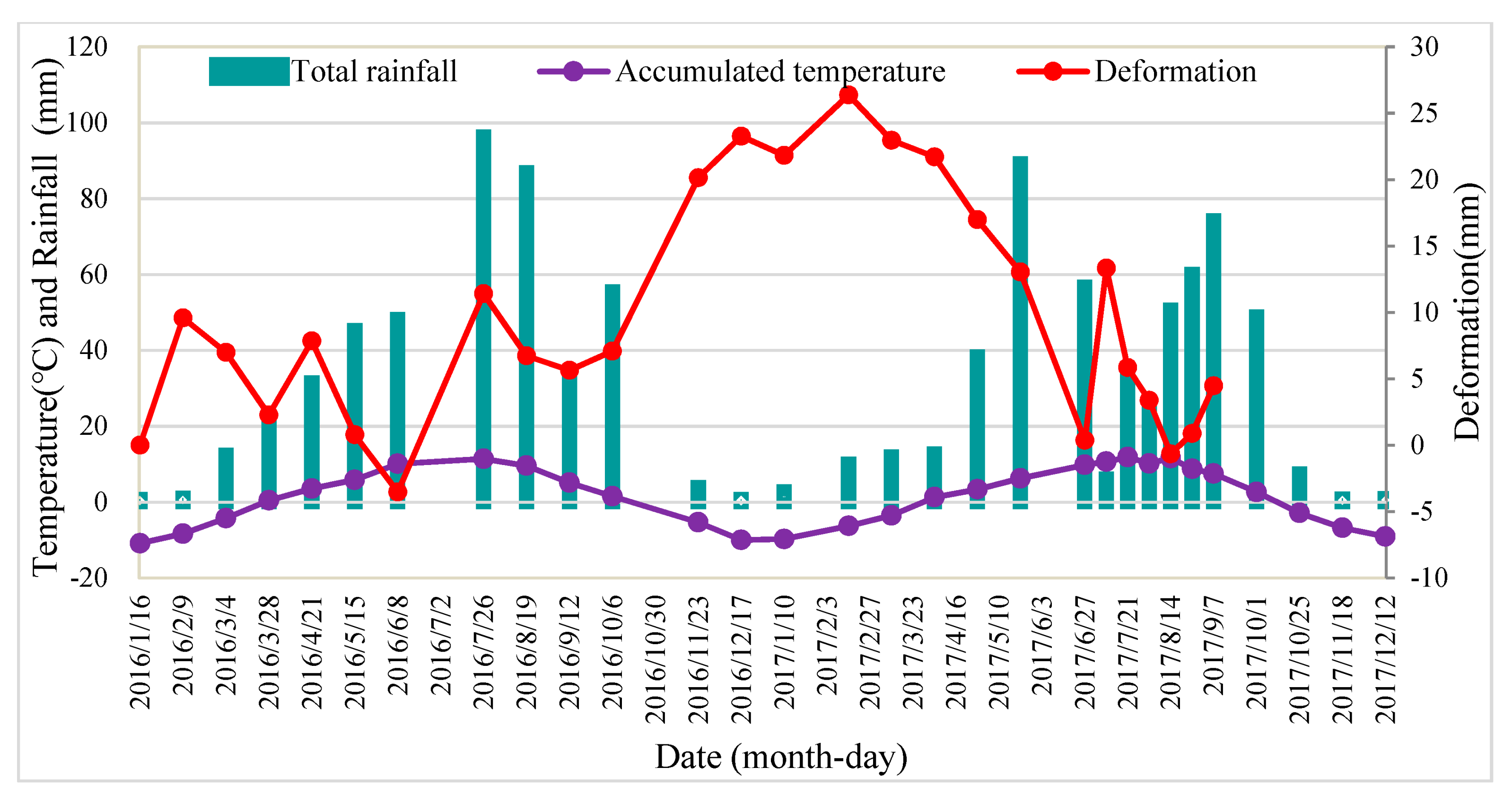
5.1. Landslide Causal Factors and Deformation Mechanism
5.2. Quantifying Landslide Activity and InSAR Signal Separation
5.3. InSAR Technique Using in Frozen Ground
6. Conclusions
Supplementary Materials
Author Contributions
Funding
Acknowledgments
Conflicts of Interest
References
- Yao, T.; Xue, Y.; Chen, D.; Chen, F.; Thompson, L.; Cui, P.; Koike, T.; Lau, W.K.M.; Lettenmaier, D.; Mosbrugger, V.; et al. Recent third pole’s rapid warming accompanies cryospheric melt and water cycle intensification and interactions between monsoon and environment: Multidisciplinary approach with observations, modeling, and analysis. Bull. Am. Meteorol. Soc. 2018, 100, 423–444. [Google Scholar] [CrossRef]
- Chen, D.; Xu, B.; Yao, T.; Guo, Z.; Cui, P.; Chen, F.; Zhang, R.; Zhang, X.; Zhang, Y.; Fan, J.; et al. Assessment of past, present and future environmental changes on the Tibetan Plateau. Chin. Sci. Bull. 2015, 60, 3025–3035. [Google Scholar]
- Cui, P.; Jia, Y. Mountain hazards in the Tibetan Plateau: Research status and prospects. Natl. Sci. Rev. 2015, 2, 397–399. [Google Scholar] [CrossRef]
- Ding, Y.; Zhang, S.; Zhao, L.; Li, Z.; Kang, S. Global warming weakening the inherent stability of glaciers and permafrost. Sci. Bull. 2019, 64, 245–253. [Google Scholar] [CrossRef] [Green Version]
- Sun, Z.; Wang, Y.; Sun, Y.; Niu, F.; Li, G.; Gao, Z. Creep characteristics and process analyses of a thaw slump in the permafrost region of the Qinghai-Tibet Plateau, China. Geomorphology 2017, 293, 1–10. [Google Scholar] [CrossRef]
- Ward Jones, M.K.; Pollard, W.H.; Jones, B.M. Rapid initialization of retrogressive thaw slumps in the Canadian high Arctic and their response to climate and terrain factors. Environ. Res. Lett. 2019, 14, 055006. [Google Scholar] [CrossRef]
- Gao, Z.; Niu, F.; Wang, Y.; Luo, J.; Lin, Z. Impact of a thermokarst lake on the soil hydrological properties in permafrost regions of the Qinghai-Tibet Plateau, China. Sci. Total Environ. 2017, 574, 751–759. [Google Scholar] [CrossRef]
- Yang, M.; Wang, X.; Pang, G.; Wan, G.; Liu, Z. The Tibetan Plateau cryosphere: Observations and model simulations for current status and recent changes. Earth Sci. Rev. 2019, 190, 353–369. [Google Scholar] [CrossRef]
- Cheng, G.; Wu, T. Responses of permafrost to climate change and their environmental significance, Qinghai-Tibet Plateau. J. Geophys. Res. Earth Surf. 2007, 112, 1–10. [Google Scholar] [CrossRef]
- Zhao, L.; Marchenko, S.S.; Sharkhuu, N.; Wu, T. Regional changes of permafrost in Central Asia Qinghai-Tibet Plateau in China. Proc. Ninth Int. Conf. Permafr. 2008, 29, 2061–2069. [Google Scholar]
- The International Disaster Database. Available online: https://www.emdat.be/database (accessed on 10 April 2019).
- Lin, Q.; Wang, Y. Spatial and temporal analysis of a fatal landslide inventory in China from 1950 to 2016. Landslides 2018, 15, 2357–2372. [Google Scholar] [CrossRef]
- Mikosš, M.; Casagli, N.; Yin, Y.; Sassa, K. Advancing Culture of Living with Landslides: Volume 1 ISDR-ICL Sendai Partnerships 2015–2025; Springer: Berlin/Heidelberg, Germany, 2017; Volume 5, ISBN 3319534858. [Google Scholar]
- Bowman, E.T. Small Landslides-Frequent, Costly, and Manageable; Elsevier Inc: Amsterdam, The Netherlands, 2014; ISBN 9780123964755. [Google Scholar]
- Luo, J.; Yin, G.; Niu, F.; Lin, Z.; Liu, M. High spatial resolution modeling of climate change impacts on permafrost thermal conditions for the Beiluhe Basin, Qinghai-Tibet Plateau. Remote Sens. 2019, 11, 1294. [Google Scholar] [CrossRef]
- Wu, Q.; Shi, B.; Fang, H.Y. Engineering geological characteristics and processes of permafrost along the Qinghai-Xizang (Tibet) Highway. Eng. Geol. 2003, 68, 387–396. [Google Scholar] [CrossRef]
- Leandro, G.; Mucciarelli, M.; Pellicani, R.; Spilotro, G. Monitoring of large instable areas: System reliability and new tools. EGU Gen. Assem. Conf. Abstr. 2009, 11, 10961. [Google Scholar]
- Metternicht, G.; Hurni, L.; Gogu, R. Remote sensing of landslides: An analysis of the potential contribution to geo-spatial systems for hazard assessment in mountainous environments. Remote Sens. Environ. 2005, 98, 284–303. [Google Scholar] [CrossRef]
- Zhao, C.; Lu, Z. Remote sensing of landslides—A review. Remote Sens. 2018, 10, 8–13. [Google Scholar] [CrossRef]
- Mora, O.; Liu, J.; Lenzano, M.; Toth, C.; Grejner-Brzezinska, D. Small landslide susceptibility and hazard assessment based on airborne lidar data. Photogramm. Eng. Remote Sens. 2015, 81, 239–247. [Google Scholar] [CrossRef]
- Holec, J.; Bednarik, M.; Šabo, M.; Minár, J.; Yilmaz, I.; Marschalko, M. A small-scale landslide susceptibility assessment for the territory of Western Carpathians. Nat. Hazards 2013, 69, 1081–1107. [Google Scholar] [CrossRef]
- Fernández, T.; Pérez, J.; Colomo, C.; Cardenal, J.; Delgado, J.; Palenzuela, J.; Irigaray, C.; Chacón, J. Assessment of the evolution of a landslide using digital photogrammetry and LiDAR techniques in the Alpujarras Region (Granada, Southeastern Spain). Geosciences 2017, 7, 32. [Google Scholar] [CrossRef]
- Caris, J.P.T.; Van Asch, T.W.J. Geophysical, geotechnical and hydrological investigations of a small landslide in the French Alps. Eng. Geol. 1991, 31, 249–276. [Google Scholar] [CrossRef]
- Bovenga, F.; Pasquariello, G.; Pellicani, R.; Refice, A.; Spilotro, G. Landslide monitoring for risk mitigation by using corner reflector and satellite SAR interferometry: The large landslide of Carlantino (Italy). Catena 2017, 151, 49–62. [Google Scholar] [CrossRef]
- Carlà, T.; Tofani, V.; Lombardi, L.; Raspini, F.; Bianchini, S.; Bertolo, D.; Thuegaz, P.; Casagli, N. Combination of GNSS, satellite InSAR, and GBInSAR remote sensing monitoring to improve the understanding of a large landslide in high alpine environment. Geomorphology 2019, 335, 62–75. [Google Scholar] [CrossRef]
- Calò, F.; Calcaterra, D.; Iodice, A.; Parise, M.; Ramondini, M. Assessing the activity of a large landslide in southern Italy by ground-monitoring and SAR interferometric techniques. Int. J. Remote Sens. 2012, 33, 3512–3530. [Google Scholar] [CrossRef]
- Qi, S.; Zou, Y.; Wu, F.; Yan, C.; Fan, J.; Zang, M.; Zhang, S.; Wang, R. A recognition and geological model of a deep-seated ancient landslide at a reservoir under construction. Remote Sens. 2017, 9, 383. [Google Scholar] [CrossRef]
- Strozzi, T.; Klimeš, J.; Frey, H.; Caduff, R.; Huggel, C.; Wegmüller, U.; Rapre, A.C. Satellite SAR interferometry for the improved assessment of the state of activity of landslides: A case study from the Cordilleras of Peru. Remote Sens. Environ. 2018, 217, 111–125. [Google Scholar] [CrossRef] [Green Version]
- Barboux, C.; Strozzi, T.; Delaloye, R.; Wegmüller, U.; Collet, C. Mapping slope movements in Alpine environments using TerraSAR-X interferometric methods. ISPRS J. Photogramm. Remote Sens. 2015, 109, 178–192. [Google Scholar] [CrossRef] [Green Version]
- Corsini, A.; Farina, P.; Antonello, G.; Barbieri, M.; Casagli, N.; Coren, F.; Guerri, L.; Ronchetti, F.; Sterzai, P.; Tarchi, D. Space-borne and ground-based SAR interferometry as tools for landslide hazard management in civil protection. Int. J. Remote Sens. 2006, 27, 2351–2369. [Google Scholar] [CrossRef]
- Berti, M.; Corsini, A.; Franceschini, S.; Iannacone, J.P. Automated classification of persistent scatterers interferometry time series. Nat. Hazards Earth Syst. Sci. 2013, 13, 1945–1958. [Google Scholar] [CrossRef]
- Colesanti, C.; Wasowski, J. Investigating landslides with space-borne synthetic aperture radar (SAR) interferometry. Eng. Geol. 2006, 88, 173–199. [Google Scholar] [CrossRef]
- Ferretti, A.; Prati, C.; Rocca, F.; Politecnico, I. Permanent scatterers in SAR interferometry. IEEE Trans. Geosci. Remote Sens. 1999, 39, 1528–1530. [Google Scholar]
- Berardino, P.; Fornaro, G.; Lanari, R.; Sansosti, E. A new algorithm for surface deformation monitoring based on small baseline differential SAR interferograms. IEEE Trans. Geosci. Remote Sens. 2002, 40, 2375–2383. [Google Scholar] [CrossRef] [Green Version]
- Barboux, C.; Delaloye, R.; Lambiel, C. Inventorying slope movements in an Alpine environment using DInSAR. Earth Surf. Process. Landforms 2014, 39, 2087–2099. [Google Scholar] [CrossRef] [Green Version]
- Zhou, X.; Chang, N.B; Li, S. Applications of SAR interferometry in earth and environmental science research. Sensors 2009, 9, 1876–1912. [Google Scholar] [CrossRef]
- The Copernicus Open Access Hub. Available online: https://scihub.copernicus.eu/dhus/#/home (accessed on 3 September 2018).
- Yin, Y.; Ma, Y.; Ma, Y.; Hu, D.; Zhang, Z. Rapid Identification and Emergency Investigation of Surface Ruptures and Geohazards Induced by the Ms 7.1 Yushu Earthquake. J. Eng. Geol. 2010, 84, 289–296. [Google Scholar]
- Zhang, X. Snow Monitoring and Early Warning of Snow Disaster in Pastoral Areas of Qinghai Province. Ph.D. Thesis, Lanzhou University, Lanzhou, China, 2016. [Google Scholar]
- Zou, D.; Zhao, L.; Sheng, Y.; Chen, J.; Hu, G.; Wu, T.; Wu, J.; Xie, C.; Wu, X.; Pang, Q.; et al. A new map of permafrost distribution on the Tibetan Plateau. Cryosphere 2017, 11, 2527–2542. [Google Scholar] [CrossRef] [Green Version]
- Gao, B.; Wang, J.; Zhang, C.; Feng, W. Formation mechanism of rainstorm-induced debris flow in Yushu state of Qinghai Province-a case study on debris flow of Lalong Gully in Chengduo county. Bull. Soil Water Conserv. 2016, 36, 28–31. [Google Scholar]
- Zhimei Landslide. Available online: http://www.yushunews.com/system/2017/09/09/012410991.shtml (accessed on 9 September 2017).
- Zhimei Landslide(Video). Available online: http://www.jiaomomo.com/forum.php?mod=viewthread& tid=353932 (accessed on 9 September 2017).
- Highland, L.M.; Bobrowski, P. The Landslide Handbook—A Guide to Understanding Landslides; US Geological Survey Circular: Reston, VA, USA, 2008; Volume 1325, p. 129.
- The United States Geological Survey, USGS. Available online: http://earthexplorer.usgs.gov/ (accessed on 3 September 2018).
- PHANTOM 4 PRO. Available online: https://www.dji.com/cn/phantom-4-pro (accessed on 3 September 2018).
- Doin, M.P.; Lasserre, C.; Peltzer, G.; Cavalié, O.; Doubre, C. Corrections of stratified tropospheric delays in SAR interferometry: Validation with global atmospheric models. J. Appl. Geophys. 2009, 69, 35–50. [Google Scholar] [CrossRef]
- Daout, S.; Doin, M.; Peltzer, G.; Socquet, A.; Lasserre, C. Large scale InSAR monitoring of permafrost freeze-thaw cycles on the Tibetan Plateau. Geophys. Res. Lett. 2017, 44, 1–16. [Google Scholar] [CrossRef]
- Sentinel-1 Quality Control. Available online: https://qc.sentinel1.eo.esa.int/ (accessed on 3 September 2018).
- Zhang, L.; Ding, X.; Lu, Z.; Jung, H.S.; Hu, J.; Feng, G. A novel multitemporal insar model for joint estimation of deformation rates and orbital errors. IEEE Trans. Geosci. Remote Sens. 2014, 52, 3529–3540. [Google Scholar] [CrossRef]
- Ducret, G.; Doin, M.P.; Grandin, R.; Lasserre, C.; Guillaso, S. DEM corrections before unwrapping in a small baseline strategy for InSAR time series analysis. IEEE Geosci. Remote Sens. Lett. 2013, 11, 696–700. [Google Scholar] [CrossRef]
- Ferretti, A. Satellite InSAR Data—Reservoir Monitoring from Space; EAGE: Houten, The Netherlands, 2014; Volume 3, ISBN 9789073834712. [Google Scholar]
- Wang, L.; Marzahn, P.; Bernier, M.; Jacome, A.; Poulin, J.; Ludwig, R. Comparison of TerraSAR-X and ALOS PALSAR differential interferometry with multisource DEMs for monitoring ground displacement in a discontinuous permafrost region. IEEE J. Sel. Top. Appl. Earth Obs. Remote Sens. 2017, 10, 4074–4093. [Google Scholar] [CrossRef]
- Pepe, A.; Lanari, R. On the extension of the minimum cost flow algorithm for phase unwrapping of multitemporal differential SAR interferograms. IEEE Trans. Geosci. Remote Sens. 2006, 44, 2374–2383. [Google Scholar] [CrossRef]
- Zuo, J.; Gong, H.; Chen, B.; Liu, K.; Zhou, C.; Ke, Y. Time-series evolution patterns of land subsidence in the Eastern Beijing Plain, China. Remote Sens. 2019, 11, 539. [Google Scholar] [CrossRef]
- Wang, C.; Zhang, Z.; Zhang, H.; Zhang, B.; Tang, Y.; Wu, Q. Active layer thickness retrieval of Qinghai-Tibet permafrost using the TerraSAR-X InSAR Technique. IEEE J. Sel. Top. Appl. Earth Obs. Remote Sens. 2018, 11, 4403–4413. [Google Scholar] [CrossRef]
- Liu, L.; Schaefer, K.; Zhang, T.; Wahr, J. Estimating 1992–2000 average active layer thickness on the Alaskan North Slope from remotely sensed surface subsidence. J. Geophys. Res. Earth Surf. 2012, 117, 1–14. [Google Scholar] [CrossRef]
- Hu, G.; Zhao, L.; Wu, X.; Li, R.; Wu, T.; Xie, C.; Qiao, Y.; Shi, J.; Li, W.; Cheng, G. New Fourier-series-based analytical solution to the conduction-convection equation to calculate soil temperature, determine soil thermal properties, or estimate water flux. Int. J. Heat Mass Transf. 2016, 95, 815–823. [Google Scholar] [CrossRef]
- Visser, V.; Langdon, B.; Pauchard, A.; Richardson, D.M. Unlocking the potential of google earth as a tool in invasion science. Biol. Invasions 2014, 16, 513–534. [Google Scholar] [CrossRef]
- Gansu Data and Application Center for High-resolution Earth Observation System. Available online: http://www.westgfdc.ac.cn/sysMng/ (accessed on 12 September 2017).
- The China Meteorological Administration. Available online: http://data.cma.cn (accessed on 3 September 2018).
- Zou, Q.; Cui, P.; He, J.; Lei, Y.; Li, S. Regional risk assessment of debris flows in China—An HRU-based approach. Geomorphology 2019, 340, 84–102. [Google Scholar] [CrossRef]
- Bogaard, T.A.; Greco, R. Landslide hydrology: From hydrology to pore pressure. Wiley Interdiscip. Rev. Water 2016, 3, 439–459. [Google Scholar] [CrossRef]
- Yalcin, A. GIS-based landslide susceptibility mapping using analytical hierarchy process and bivariate statistics in Ardesen (Turkey): Comparisons of results and confirmations. CATENA 2008, 72, 1–12. [Google Scholar] [CrossRef]
- Schmidt, D.A.; Bürgmann, R. Time-dependent land uplift and subsidence in the Santa Clara valley, California, from a large interferometric synthetic aperture radar data set. J. Geophys. Res. Solid Earth 2003, 108, 1–13. [Google Scholar] [CrossRef]
- Sun, Q.; Zhang, L.; Ding, X.L.; Hu, J.; Li, Z.W.; Zhu, J.J. Slope deformation prior to Zhouqu, China landslide from InSAR time series analysis. Remote Sens. Environ. 2015, 156, 45–57. [Google Scholar] [CrossRef]
- Carlà, T.; Farina, P.; Intrieri, E.; Ketizmen, H.; Casagli, N. Integration of ground-based radar and satellite InSAR data for the analysis of an unexpected slope failure in an open-pit mine. Eng. Geol. 2018, 235, 39–52. [Google Scholar] [CrossRef]
- Zhao, L.; Cheng, G.; Shuxun, L.I.; Zhao, X.; Wang, S. Thawing and freezing processes of active layer in Wudaoliang region of Tibetan Plateau. Sci. Bull. 2000, 45, 2181–2187. [Google Scholar] [CrossRef]
- Darrow, M.M.; Daanen, R.P.; Gong, W. Predicting movement using internal deformation dynamics of a landslide in permafrost. Cold Reg. Sci. Technol. 2017, 143, 93–104. [Google Scholar] [CrossRef]
- Xu, J.; Wang, Z.Q; Ren, J.W; Wang, S.H; Jin, L. Mechanism of slope failure in loess terrains during spring thawing. J. Mt. Sci. 2018, 15, 845–858. [Google Scholar] [CrossRef]
- Lopez, S.J.; Corona, C.; Stoffel, M.; Berger, F. Climate change increases frequency of shallow spring landslides in the French Alps. Geology 2013, 41, 619–622. [Google Scholar]
- Bíl, M.; Müller, I. The origin of shallow landslides in Moravia (Czech Republic) in the spring of 2006. Geomorphology 2008, 99, 246–253. [Google Scholar] [CrossRef]
- Moreiras, S.; Lisboa, M.S.; Mastrantonio, L. The role of snow melting upon landslides in the central Argentinean Andes. Earth Surf. Process. Landforms 2012, 37, 1106–1119. [Google Scholar] [CrossRef]
- Balser, A.W.; Gens, R.; Member, A.C.; Mack, M.C.; Member, A.C.; Walker, D.A.; Member, A.C.; Wagner, D.; Layer, P.W.; Eichelberger, J.C. Retrogressive Thaw Slumps and Active Layer Detachment Slides in the Brooks Range and Foothills of Northern Alaska Terrain and Timing. Ph.D. Thesis, University of Alaska Fairbanks, Fairbanks, AK, USA, 2015. [Google Scholar]
- Lewkowicz, A.G.; Way, R.G. Extremes of summer climate trigger thousands of thermokarst landslides in a high arctic environment. Nat. Commun. 2019, 10, 1–11. [Google Scholar] [CrossRef]
- Swanson, D.K.; Nolan, M. Growth of retrogressive thaw slumps in the Noatak Valley, Alaska, 2010–2016, measured by airborne photogrammetry. Remote Sens. 2018, 10, 2010–2016. [Google Scholar] [CrossRef]
- Zwieback, S.; Kokelj, S.; Günther, F.; Boike, J.; Grosse, G.; Hajnsek, I. Sub-seasonal thaw slump mass wasting is not consistently energy limited at the landscape scale. Cryosphere 2018, 12, 549–564. [Google Scholar] [CrossRef] [Green Version]
- Luo, J.; Niu, F.; Lin, Z.; Liu, M.; Yin, G. Recent acceleration of thaw slumping in permafrost terrain of Qinghai-Tibet Plateau: An example from the Beiluhe Region. Geomorphology 2019, 341, 79–85. [Google Scholar] [CrossRef]
- Zhang, X.; Zhang, H.; Wang, C.; Tang, Y.; Zhang, B.; Wu, F.; Wang, J.; Zhang, Z. Time-series InSAR monitoring of permafrost freeze-thaw seasonal displacement over Qinghai-Tibetan Plateau using sentinel-1 data. Remote Sens. 2019, 11, 1000. [Google Scholar] [CrossRef]
- Whiteley, J.S.; Chambers, J.E.; Uhlemann, S.; Wilkinson, P.B.; Kendall, J.M. Geophysical monitoring of moisture-induced landslides: A review. Rev. Geophys. 2019, 57, 106–145. [Google Scholar] [CrossRef]
- Barra, A.; Monserrat, O.; Mazzanti, P.; Esposito, C.; Crosetto, M.; Scarascia Mugnozza, G. First insights on the potential of Sentinel-1 for landslides detection. Geomatics Nat. Hazards Risk 2016, 7, 1874–1883. [Google Scholar] [CrossRef] [Green Version]
- Strozzi, T.; Antonova, S.; Günther, F.; Mätzler, E.; Vieira, G.; Wegmüller, U.; Westermann, S.; Bartsch, A. Sentinel-1 SAR interferometry for surface deformation monitoring in low-land permafrost areas. Remote Sens. 2018, 10, 1360. [Google Scholar] [CrossRef]
- Michaelides, R.J.; Schaefer, K.; Zebker, H.A.; Parsekian, A.; Liu, L.; Chen, J.; Natali, S.; Ludwig, S.; Schaefer, S.R. Inference of the impact of wildfire on permafrost and active layer thickness in a discontinuous permafrost region using the remotely sensed active layer thickness (ReSALT) algorithm. Environ. Res. Lett. 2019, 14, 035007. [Google Scholar] [CrossRef]
- Short, N.; Leblanc, A.M.; Sladen, W.; Brisco, B. RADARSAT-2 InSAR for monitoring permafrost environments: Pangnirtung and iqaluit. In Proceedings of the 2013 IEEE Radar Conference (RadarCon13), Ottawa, ON, Canada, 29 April–23 May 2013; pp. 4–7. [Google Scholar]
- Dai, K.; Liu, G.; Li, Z.; Ma, D.; Wang, X.; Zhang, B.; Tang, J.; Li, G. Monitoring highway stability in permafrost regions with X-band temporary scatterers stacking InSAR. Sensors 2018, 18, 1876. [Google Scholar] [CrossRef]
- Nolan, M.; Fatland, D.R. Penetration depth as a DInSAR observable and proxy for soil moisture. IEEE Trans. Geosci. Remote Sens. 2003, 41, 532–537. [Google Scholar] [CrossRef] [Green Version]
- Le Bivic, R.; Allemand, P.; Quiquerez, A.; Delacourt, C. Potential and limitation of SPOT-5 ortho-image correlation to investigate the cinematics of landslides: The example of Mare à Poule d’Ea” (Réunion, France). Remote Sens. 2017, 9, 106. [Google Scholar] [CrossRef]


| SAR Sensor | Sentinel-1A IW SLC |
|---|---|
| Orbit direction | Ascending |
| Microwave band (polarization) | C-band (VV) |
| Number of frames | 27 |
| Resolution | 5 m × 20 m |
| Repeat cycle | 12 days |
| Look angle | 42° |
| Temporal coverage | January 2016–September 2017 |
| Location | Dataset | Environment Condition | Reference & Validation | Time Period | Amplitude of Deformation | Factors Discussion | Authors |
|---|---|---|---|---|---|---|---|
| Arctic and Antarctic | Sentinel-1 | Low-land permafrost | In-situ, TerraSAR-X | 201711-201812 | 3–10 cm | Deformation validation | Strozzi et al. 2018 [82] |
| Eastern Canada | RadarSat-2 | Continuous permafrost | Bedrock | 201105-201109 | 0–6.5 cm | Soil moisture | Short et al. 2013 [84] |
| Southwestern Alaska | ALOS | Discontinuous permafrost | Absolute phase calculated by ALT | 200712-201002 | 0–4 cm | Wildfire | Michaelides et al. 2019 [83] |
| Northwestern Qinghai Tibet | Envisat | Discontinuous permafrost | Bedrock | 2003–2011 | 0–1.2 cm | Soil moisture | Daout et al. 2017 [48] |
| Central Qinghai-Tibet Plateau | Sentinel-1 | Permafrost region | ALT | 201711-201812 | 0.2–3 cm | Active layer, land covers | Zhang et al. 2019 [79] |
| Eastern Qinghai-Tibet Plateau | Sentinel-1 | Permafrost, seasonally frozen ground | Bedrock, high-coherence | 201601-201709 | 0–11 cm | Freeze thaw cycle, rainfall | this study area |
| Qinghai-Tibet highway(G214) | TerraSAR-X | Permafrost, seasonally frozen ground | Unkown | 201508-201508 | 0–10 cm | Freeze thaw cycle | Dai et al. 2018 [85] |
© 2019 by the authors. Licensee MDPI, Basel, Switzerland. This article is an open access article distributed under the terms and conditions of the Creative Commons Attribution (CC BY) license (http://creativecommons.org/licenses/by/4.0/).
Share and Cite
Hao, J.; Wu, T.; Wu, X.; Hu, G.; Zou, D.; Zhu, X.; Zhao, L.; Li, R.; Xie, C.; Ni, J.; et al. Investigation of a Small Landslide in the Qinghai-Tibet Plateau by InSAR and Absolute Deformation Model. Remote Sens. 2019, 11, 2126. https://doi.org/10.3390/rs11182126
Hao J, Wu T, Wu X, Hu G, Zou D, Zhu X, Zhao L, Li R, Xie C, Ni J, et al. Investigation of a Small Landslide in the Qinghai-Tibet Plateau by InSAR and Absolute Deformation Model. Remote Sensing. 2019; 11(18):2126. https://doi.org/10.3390/rs11182126
Chicago/Turabian StyleHao, Junming, Tonghua Wu, Xiaodong Wu, Guojie Hu, Defu Zou, Xiaofan Zhu, Lin Zhao, Ren Li, Changwei Xie, Jie Ni, and et al. 2019. "Investigation of a Small Landslide in the Qinghai-Tibet Plateau by InSAR and Absolute Deformation Model" Remote Sensing 11, no. 18: 2126. https://doi.org/10.3390/rs11182126