Combing Triple-Part Features of Convolutional Neural Networks for Scene Classification in Remote Sensing

Abstract

High spatial resolution remote sensing (HSRRS) images contain complex geometrical structures and spatial patterns, and thus HSRRS scene classification has become a significant challenge in the remote sensing community. In recent years, convolutional neural network (CNN)-based methods have attracted tremendous attention and obtained excellent performance in scene classification. However, traditional CNN-based methods focus on processing original red-green-blue (RGB) image-based features or CNN-based single-layer features to achieve the scene representation, and ignore that texture images or each layer of CNNs contain discriminating information. To address the above-mentioned drawbacks, a CaffeNet-based method termed CTFCNN is proposed to effectively explore the discriminating ability of a pre-trained CNN in this paper. At first, the pretrained CNN model is employed as a feature extractor to obtain convolutional features from multiple layers, fully connected (FC) features, and local binary pattern (LBP)-based FC features. Then, a new improved bag-of-view-word (iBoVW) coding method is developed to represent the discriminating information from each convolutional layer. Finally, weighted concatenation is employed to combine different features for classification. Experiments on the UC-Merced dataset and Aerial Image Dataset (AID) demonstrate that the proposed CTFCNN method performs significantly better than some state-of-the-art methods, and the overall accuracy can reach 98.44% and 94.91%, respectively. This indicates that the proposed framework can provide a discriminating description for HSRRS images.

1. Introduction

With the improvement of Earth observation technology, great progress has been made in the collection of high spatial resolution remote sensing (HSRRS) images [1,2,3]. Compared with low spatial resolution remote sensing images, an HSRRS image contains more details of ground objects and more complex spatial patterns [4,5,6,7,8]. Therefore, sub-meter level HSRRS images have been applied in many areas such as land resources planning [9,10], geospatial object detection [11,12,13], and environmental monitoring [14]. HSRRS-image-based scene classification has attracted increasing attention in the remote sensing community [15,16,17,18,19,20].

In scene classification, the extraction of scene-level discriminative features is the key step to bridging the huge gap between an original image and its semantic category. In recent years, researchers have proposed various feature extraction methods, which can be divided into three main types: low-level methods, mid-level methods, and high-level methods [21,22]. Traditional scene classification methods were developed directly based on low-level features, such as texture features, color features, spectral features, and multi-feature fusion [23,24]. However, these hand-crafted features are limited in describing complex scenes of HSRRS, which will affect the classification performance.

Compared with the low-level methods, the mid-level methods aim to obtain a global representation of a scene by encoding local descriptors, e.g., scale-invariant feature transform, histogram of oriented gradient and color histogram. The bag-of-view-word (BoVW) model is one of the most popular feature encoding approaches [25]. Due to its simplicity and efficiency, the BoVW model is widely applied for mid-level scene description [26,27,28,29]. However, the quantization error of the BoVW method is large, and some important information may be lost. Therefore, many feature coding methods were developed to reduce the reconstruction error, including improved Fisher kernel (IFK) [30], vectors of locally aggregated descriptors (VLAD) [31], spatial pyramid matching kernel (SPM) [32], locality-constrained linear coding (LLC) [33], latent semantic analysis (LSA), probabilistic latent semantic analysis (pLSA) [34,35], and latent dirichlet allocation (LDA) [35]. However, both low-level and mid-level methods are mainly based on hand-crafted features, which are difficult to effectively describe in HSRRS scene images with complex land-cover/land-use (LULC) situations.

In recent years, deep-learning-based methods have made a breakthrough in the field of machine learning [36,37], and convolutional neural networks (CNNs) have achieved excellent performance in computer vision tasks such as image segmentation [8,38], change detection [39], and image classification [40]. Based on CNNs, some significant progresses have also been proposed for HSRRS image scene classification [41,42,43,44,45,46,47,48]. Penatti et al. [49] explored the generalization ability of the pre-trained OverFeat model and CaffeNet model by using features from the last fully connected layer. Hu et al. [50] developed two schemes for extracting features from different layers of CNNs. In [51,52], collaborative representation is employed to reprocess features extracted from a pre-trained CNN. Flores et al. [53] combined the pre-trained deep CNN with a sparse representation to improve the performance of land-use classification. Li et al. [54] proposed a fusion strategy to integrate multilayer features of a pre-trained CNN model by principal component analysis (PCA) and a spectral regression kernel discriminant analysis (SRKDA) method. Chaib et al. [55] introduced a framework for scene classification by regarding pre-trained VGG-Net models as deep feature extractors, and it explored discriminant correlation analysis (DCA) to fuse features from two fully connected layers. In [21,56], a two-stream architecture was developed, and texture-coded mapped images were adopted as the second stream to provide complementary information by fusing with a raw red-green-blue (RGB) image stream. The aforementioned methods just focus on original RGB image-based features or CNN-based single-layer features to achieve the global representation of HSRRS scenes, and these methods ignore that each layer or texture image contains abundant information.

Motivated by the above-mentioned limitations, a novel feature extraction and classification framework based on a pre-trained CNN is proposed for HSRRS scene classification in this paper. The framework employs a pre-trained CNN as a feature extractor and combines triple-part features of convolutional neural networks (CTFCNN), including convolutional features from multilayers, fully connected (FC) features and local binary pattern (LBP)-based FC features to adequately explore the discriminating ability of the pre-trained CNN. In summary, the main contributions of the proposed CTFCNN method can be listed as the following:

(1) To effectively utilize the convolutional features of a pre-trained CNN, an improved bag-of-view-word (iBoVW) method is developed for representing the discriminating information from each convolutional layer.

(2) An approach is presented to integrate hand-crafted local binary pattern (LBP) texture descriptors into a pre-trained CNN, and the obtained LBP-based FC features can provide information supplements to achieve a good classification performance.

(3) A feature fusion framework CTFCNN is proposed to combine multilayer features of the CNN and LBP-based FC features by weighted concatenation.

2. Related Works

2.1. Convolutional Neural Network (CNN)

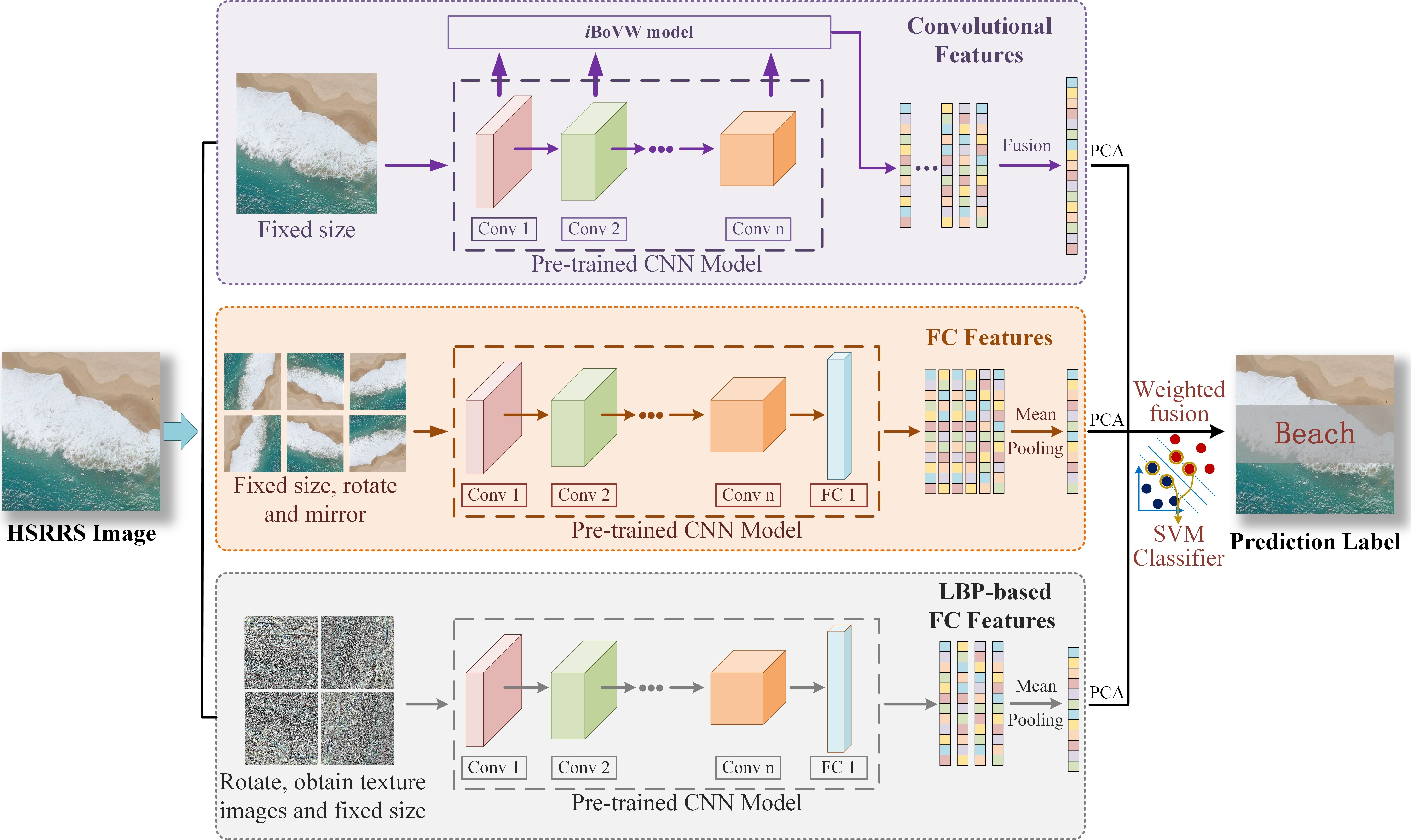
CNN is one of the most popular deep learning methods, and the main advantage is that original images can be directly input into the networks without complex pre-processing [57,58]. The typical CNNs are generally composed of convolutional layers, pooling layers, activation layers, fully-connected layers, and a softmax layer. Figure 1 shows the architecture of CaffeNet, which is a ypical CNN model [59].

As we can see from Figure 1, for an input HSRRS image, convolution computations are first performed by using convolution kernels with weight sharing, and feature maps can be obtained. Then the nonlinear activation function including rectified linear unit (ReLU) and sigmoid is introduced to enhance the expression ability. After that, mean pooling or max pooling are employed to reduce the parameters of the network and improve the translation invariance. As the depth of the layer increases, the feature maps tend to be highly abstract, and the feature maps from the last convolutional layer are flattened into a feature vector. The feature vector is further processed by the fully connected layers to form the global feature of a scene image, and it is fed into a softmax layer to gain the possibility for·each class.

2.2. Bag-of-View-Word (BoVW)

The BoVW model was originally proposed for natural language processing (NLP) and information retrieval (IR). Under this model, an image can be represented as a combination of many visual words. BoVW-based methods are widely applied in the computer vision field for simplicity and efficiency [60,61]. The main processes are summarized as follows:

(1) Local image patch sampling and feature extraction. For an input image, local image patches are obtained by dense sampling or sparse sampling. Then, local descriptors are extracted for each sampled image patch.

(2) Constructing a dictionary (codebook) that consists of many visual words. K-means clustering is usually employed to learn a set of clustering centers from local features. Each clustering center can be regarded as a visual word, and then all visual words constitute a visual dictionary.

(3) Feature encoding. Local features are mapped into dictionary space by a feature encoding method, and encoding vectors can be generated. The dimension of encoding vectors is the number of visual words. Feature coding methods include vector quantization (VQ), sparse coding (SC), and so on.

(4) Feature pooling. The global representation of an image can be formed by gathering statistics of encoding vectors. The most frequently used methods are mean pooling and max pooling.

2.3. Local Binary Pattern (LBP) Descriptor

As a typical texture descriptor, LBP [62] is widely employed in many tasks, such as face recognition [63], image classification [64], and object detection [65]. In HSRRS scene classification, texture-coded mapped images can be explored as the inputs of deep networks to provide useful supplementary information.

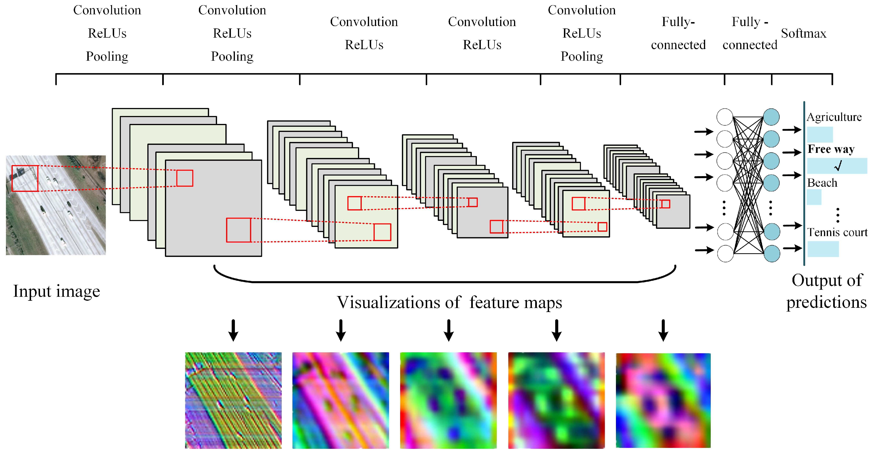
Figure 2 shows the principle of the LBP descriptor, which aims to obtain the local gray-scale distribution of an image by comparing the pixel values between the center pixel and its neighboring pixels.

As shown in Figure 2, in the $3\times 3$ spatial window, the LBP descriptor takes the gray value of the central pixel $g_0$ as the threshold and encodes by comparing $g_0$ with the gray values of eight surrounding pixels $g_i(i=1,2,\dots ,8)$. If $g_i$ is larger than $g_0$, the code of pixel $g_i$ is assigned as “1” (binary number), otherwise it is assigned as “0”. This process can be defined as

$$s\left(g_i-g_0\right)=\left\{\begin{array}{cc}1\hfill & if{g}_i\ge g_0(i=1,2,\dots ,8),\hfill \\ 0\hfill & else.\hfill \end{array}\right.$$

(1)

After LBP operation, pixel $g_c\in [0,255]$ can be obtained by clockwise connection, and it can be calculated as follows:

$$LBP\left(g_c\right)=\sum _{p=1}^{8}s\left(g_i-g_0\right)2^{p-1}.$$

(2)

3. Proposed Framework

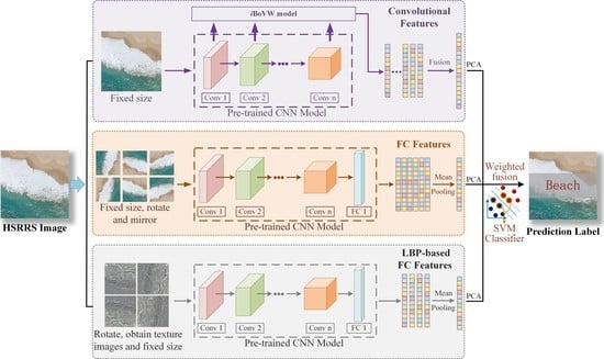
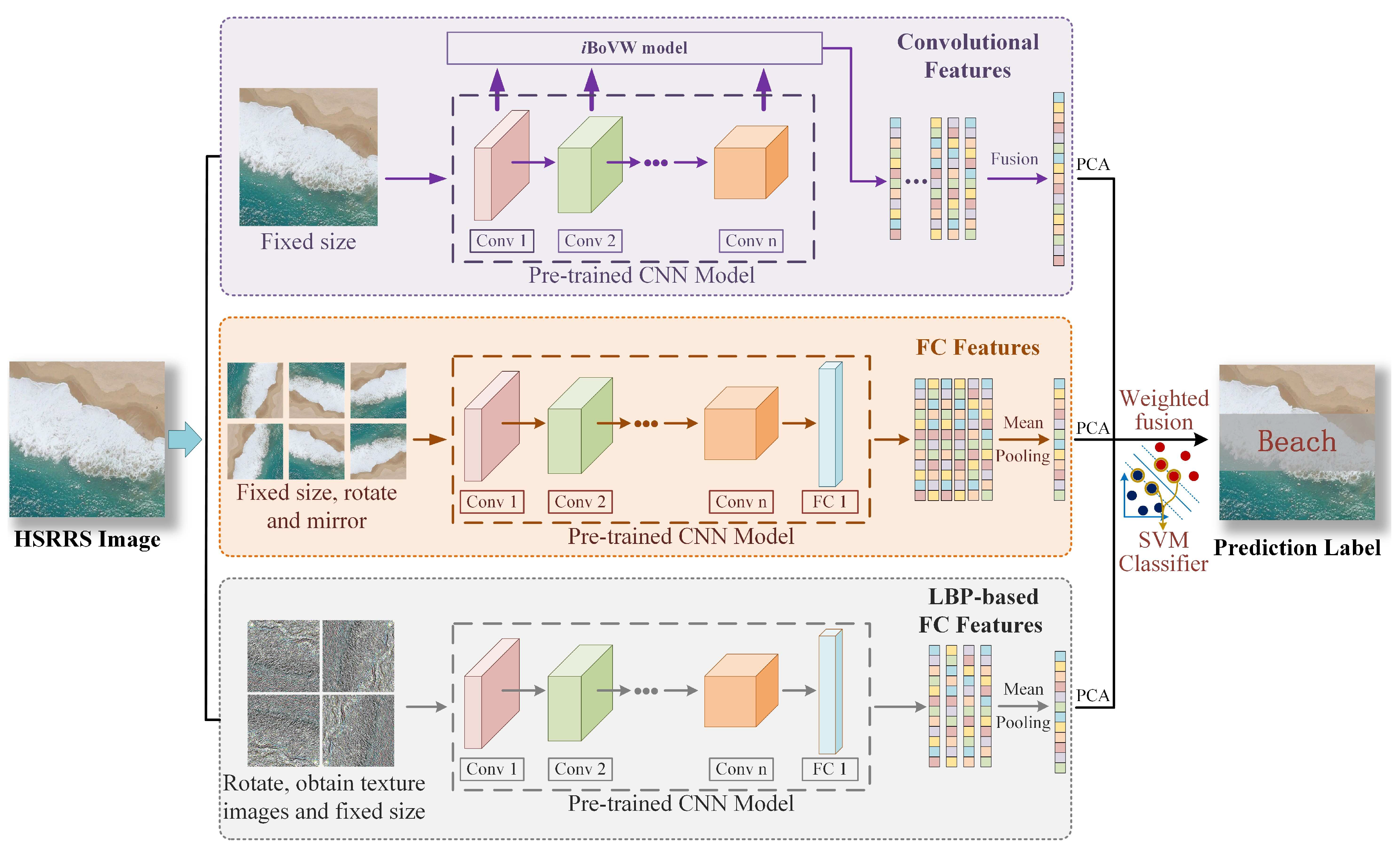
To extract the discriminating information in HSRRS images, a CaffeNet-based framework termed CTFCNN is proposed to improve the classification performance. The CTFCNN method extracts three types of features by using an off-the-shelf pre-trained CaffeNet model, and these features include multilayer convolutional features, features from fully connected layers, and LBP-based FC features. Furthermore, the operations of dimensionality reduction and feature fusion are employed to achieve an effective prediction of scene semantic category. The flowchart of the proposed CTFCNN framework is shown in Figure 3.

3.1. Convolutional Features

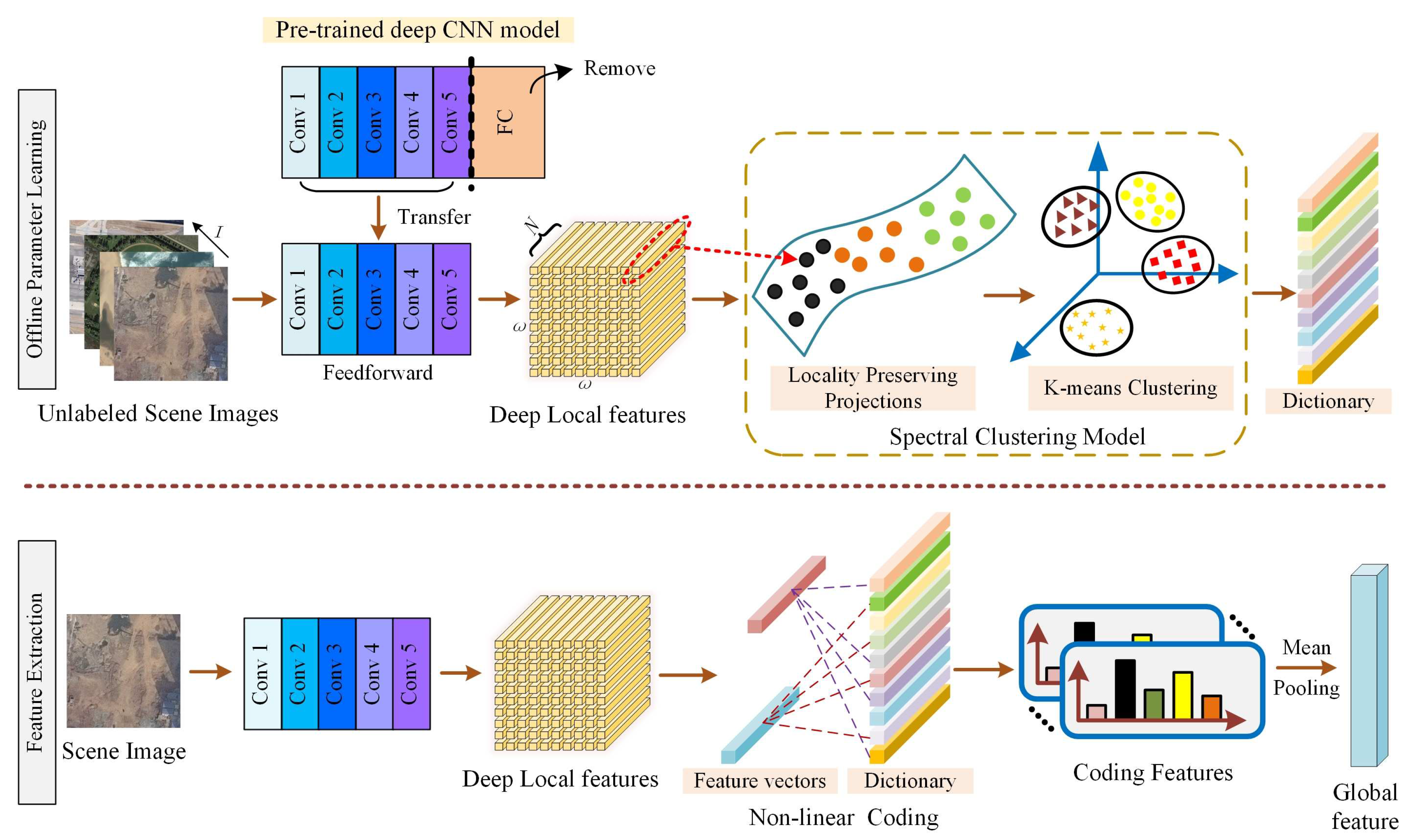
In CNNs, the feature map of each convolutional layer contains different discriminating information. To fully utilize the convolutional features of the pre-trained CNN model, a new coding method termed iBoVW is proposed to generate the features from each convolutional layer. Compared with the traditional BoVW method, iBoVW tries to achieve a more reasonable representation of a scene by fusing manifold learning and nonlinear coding. The detailed process is shown in Figure 4.

As in Figure 4, HSRRS images can be transformed into coding vectors through the iBoVW encoding operation. In detail, the iBoVW method includes offline parameter learning and feature extraction stages.

In the stage of offline parameter learning, unlabeled images are randomly chosen for the pre-trained CNN model, in which the FC layer has been removed. For each input image, the feature maps from the l-th convolutional layer can be obtained and regarded as $\omega \times \omega$ N-dimensional local features $X=\left\{x_1,x_2,\dots ,x_{{\omega }^2}\right\}\in {\Re }^N$. Then, projection matrix V and low-dimensional embedding $Y=\left\{y_1,y_2,\dots ,y_{{\omega }^2}\right\}\in {\Re }^n$ are obtained by using locality preserving projection (LPP), which aims to minimize the following objective function:

$$\left\{\begin{array}{c}min{V}^{T}XL{X}^{T}V\hfill \\ \mathrm{s}.\mathrm{t}.V^{T}XD{X}^{T}V=I,\hfill \end{array}\right.$$

(3)

where D is the diagonal weight matrix, $d_{ii}={\sum }_j{w}_{ij}$, $L=D-W$ is the Laplacian matrix, and W is the weight matrix. Then K-means clustering is performed on low-dimensional embedding Y to learn the dictionary Dic.

In the features extraction stage, the given image is input into the CNN to obtain the feature maps of the l-th convolutional layer, and projection matrix V is employed to reduce the dimension of local descriptors. Then, non-linear coding is applied for processing low-dimensional embedding Y to get coding features $\varphi$, as

$${\varphi }_i=\left\{\begin{array}{cc}\frac{1}{N_V}\sum _{c=1}^{N_V}{d}_i-d_i\hfill & \mathit{if}\frac{1}{N_V}\sum _{i=1}^{N_V}{d}_i-d_i\ge 0\&Di{c}_i\in N\left(y\right)\hfill \\ 0\hfill & \mathit{otherwise},\hfill \end{array}\right.$$

(4)

$$\varphi =\frac{\varphi -max\left(\varphi \right)}{max\left(\varphi \right)-min\left(\varphi \right)},$$

(5)

in which y is the input vector, $N_V$ denotes the size of the visual vocabulary in the dictionary, $d_i={∥y-Di{c}_i∥}_2$ denotes the Euclidean distance between y and $Di{c}_i$, $N_k(•)$ represents the k-nearest neighbors space, and k represents the number of associations between local descriptors and the visual vocabulary. $\mathrm{Max}(•)$ and $\min (•)$ represent calculating the maximum and minimum values, respectively.

Mean pooling is used to process all coding features of a scene, and deep global features from each convolutional layer can be obtained. Then, partial features are selected and fused by weighted concatenation as

$$\mathrm{conv}-fu=\left[\mathrm{conv}i,p_1\times \mathrm{conv}i+1,\dots ,p_2\times \mathrm{conv},l\right]$$

(6)

where p denotes the coefficient weight of different features, and conv (l) is the feature of the l-th convolutional layer.

3.2. Features from the Fully Connected Layer

In the phase of FC feature extraction, the pre-trained CNN model is employed as a feature extractor. Before feeding the HSRRS images to the model, each image should be adjusted to the fixed size. In the CTFCNN framework, the response from the first FC layer is extracted and regarded as the feature representation of a scene.

Data augmentation is a common technique in deep learning. Each input image is transformed to expand the number of samples, including rotating (${90}^{\circ }$, ${180}^{\circ }$, and ${270}^{\circ }$) and flipping (horizontal and vertical). Then, the mean pooling method is employed to process the obtained six FC features to get FC-aug features; the correspondence is shown in Figure 3.

3.3. CNN-Based LBP Features

In HSRRS scene classification, LBP descriptors are usually integrated with feature coding models to achieve the representation of each image. However, these traditional LBP-based methods have limited discriminating ability in highly complex HSRRS images. Due to the powerful discrimination ability of deep neural networks, the LBP descriptor is integrated with the CNN model to make full use of the texture features of images and provide complementary information to the standard RGB deep model. Because the LBP descriptor is not suitable for direct input to the pre-trained CNN model, a new pre-processed solution is proposed to extract LBP-based FC (LBPFC) features.

Each channel of original images can be regarded as a gray image and generates a texture image through the LBP descriptor described in Section 2.3. Then, these texture images are superimposed to synthesize one image that contains three channels. Furthermore, the new obtained texture image needs to be adjusted to the fixed size. As for data augmentation, only rotation transformation (${90}^{\circ }$, ${180}^{\circ }$, and ${270}^{\circ }$) is performed. After obtaining four LBPFC features, the mean pooling method is used to achieve the global representations of images as well.

3.4. Feature Fusion and Classification

After extracting different types of features from the CNN, it is crucial to effectively fuse these features for classification. Due to the high dimensionality of the features, PCA is first employed to avoid the curse of dimensionality. After normalization, a weighted concatenation method is applied for the features as follows:

$$CTFCNN=\left[\mathrm{conv}-fu,q_1\times FC-aug,q_2\times LBPFC-aug\right],$$

(7)

in which $q_1$, $q_2$ denote the coefficient weight of different features, respectively.

Finally, the linear support vector machine (SVM) classifier is employed to predict the label of samples.

4. Experiments and Discussion

In this section, two public datasets are employed to evaluate our proposed methods, and the performance of scene classification is compared with some state-of-the-art algorithms.

4.1. Dataset Description

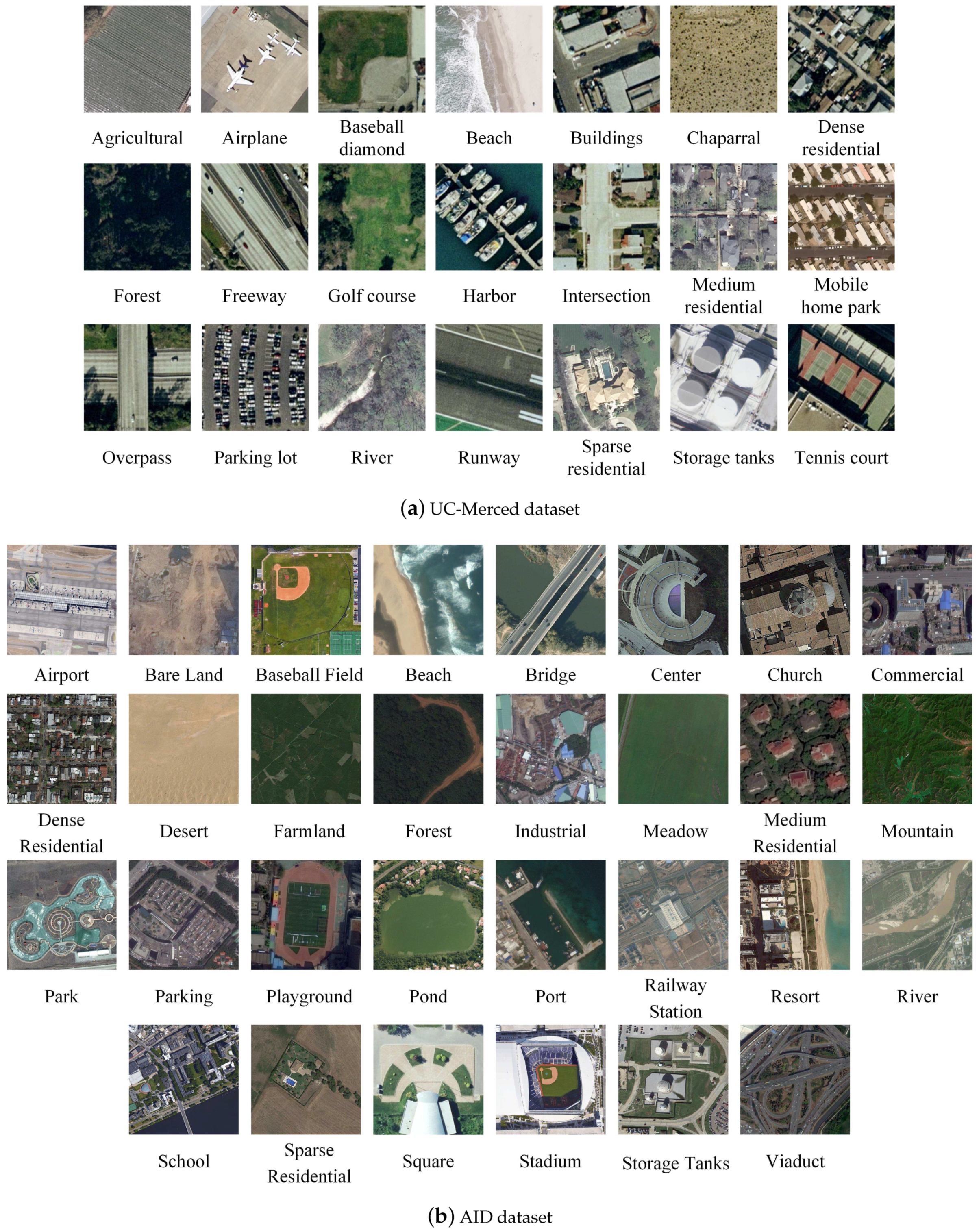
(1) UC Merced Land Use Dataset (UC-Merced dataset) [25]: The original images of this dataset were collected on the national map provided by the US Geological Survey. The dataset contains a total of 2100 images with a size of $256\times 256$ pixels, and the spatial resolution is about 0.3 m. It is divided into 21 land-use scenes classes, such as agricultural, airplane, baseball diamond, and buildings. The UC-Merced dataset is difficult to classify because it contains a large number of similar land-use types, such as dense residential, medium residential, and sparse residential. As a public dataset, it is widely adopted to evaluate scene classification methods in remote sensing fields. Figure 5a shows example images for all categories. Details about the UC-Merced dataset can be obtained at http://vision.ucmerced.edu/datasets/.

(2) Aerial Image Dataset (AID dataset) [22]: The dataset was collected by Wuhan University in Google Earth imagery. Each scene has $600\times 600$ pixels, and the spatial resolution of its images are from 0.5 m to 8 m. The dataset contains a total of 10,000 images, which are divided into 30 semantic categories as in Figure 5b. The number of scene images per class ranges from 220 to 420, including airport, bare land, baseball field, and beach; the details are shown in

Table 1. The number of scene images per class in the Aerial Image Dataset (AID).

Name	♯ of Images	Name	♯ of Images	Name ♯ of Images
airport	360	farmland	370	port	380
bare land	310	forest	250	railway station	260
baseball field	220	industrial	390	resort	290
beach	400	meadow	280	river	410
bridge	360	medium residential	290	school	300
center	260	mountain	340	sparse residential	300
church	240	park	350	square	330
commercial	350	parking	390	stadium	290
dense residential	410	playground	370	storage tanks	360
desert	300	pond	420	viaduct	420

. Since the AID is taken from different sensors, different countries, at different times, and in different seasons, the intraclass diversity of the AID is rapidly increasing. In addition, this dataset has smaller interclass dissimilarity as well. Details about the AID are available at http://captain.whu.edu.cn/project/AID/.

4.2. Experimental Setup

In each experiment, the dataset was randomly divided into training and test sets. In the UC-Merced dataset, 80% of samples were used for training, and the rest of the samples were employed for testing. In the AID, the ratio of training samples was set to 50%. After feature extraction, the public LIBLINEAR library [66] was employed to training the linear SVM classifier, and the penalty term C was tuned by a grid search with a given set $\left\{2^{-10},2^{-9},\dots ,2^9,2^{10}\right\}$. Overall accuracy (OA) with standard deviation (STD) and confusion matrix were adopted to evaluate the performance of scene classification, and experiments were repeated 20 times in each condition.

In the phase of convolutional feature extraction, each image of the two datasets ws resized to $300\times 300$ pixels to get the appropriate size of feature maps. Then, features from each convolutional layer could be obtained by CaffeNet with sizes of $73\times 73\times 96$, $36\times 36\times 256$, $18\times 18\times 384$, $18\times 18\times 384$, and $18\times 18\times 256$. As for FC features and LBP-based FC features, the images were adjusted to $227\times 227$ pixels before putting them into the CaffeNet, and a 4096-dimensional feature was extracted from the first FC layer.

All experiments were performed on a personal computer equipped with 16-GB memory, i5-8500 CPU, and 64-bit Windows 10 using MATLAB 2016a. The MATLAB toolbox called MatConvNet [67] was employed to exact different CNN features. The off-the-shelf CaffeNet [59] trained on the ImageNet Large Scale Visual Recognition Challenge (ILSVRC) dataset can be download at http://www.vlfeat.org/matconvnet/pretrained/.

4.3. Parameter Evaluation

The CTFCNN method contains several hyper-parameters, including a visual vocabulary of a certain size $N_V$ and embedding dimension d of deep local features. In this section, we describe experiments conducted to evaluate the influence of hyper-parameters on classification performance.

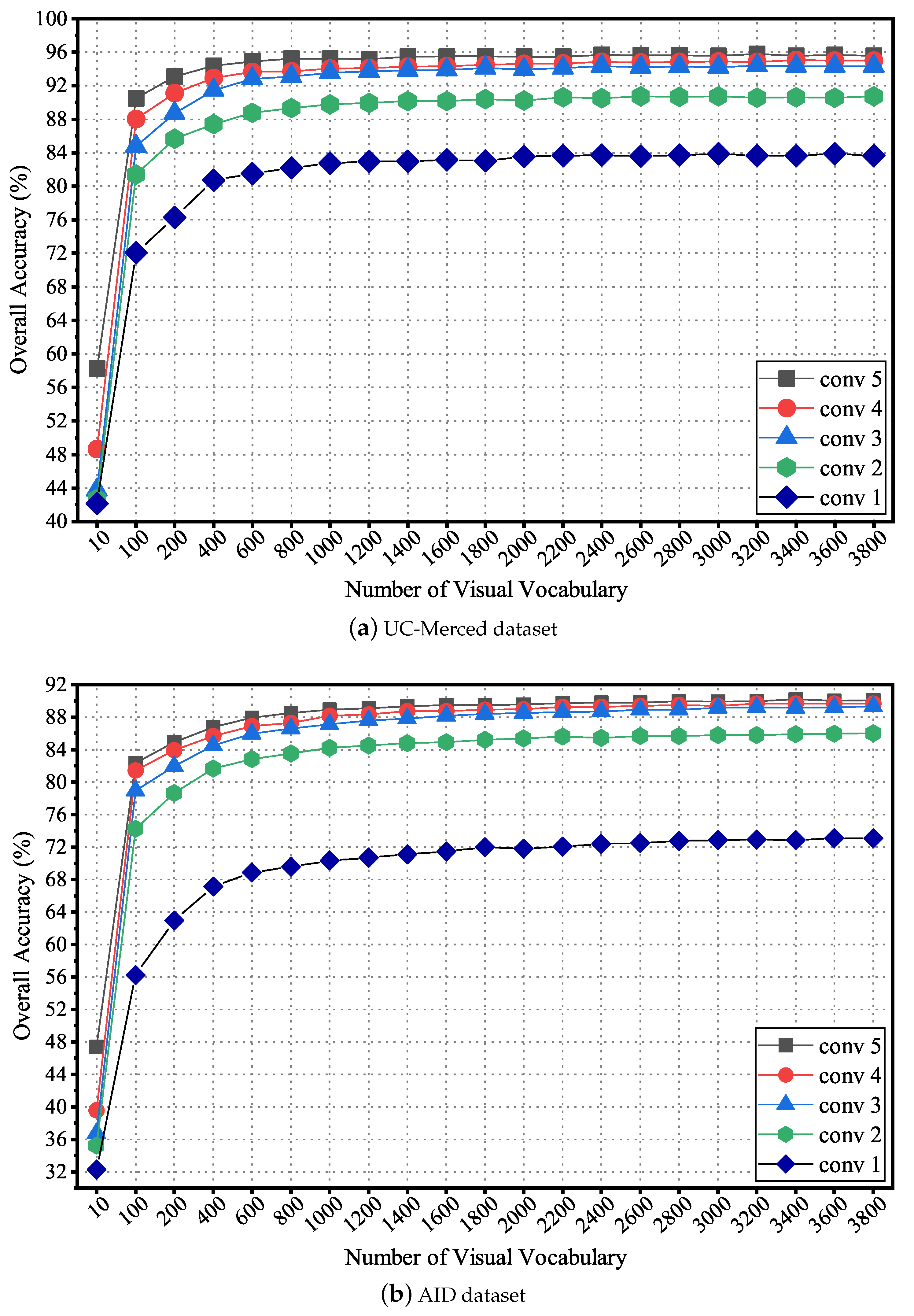
To explore the classification performance with different sizes of visual vocabulary in iBoVW coding, each convolutional layer was discussed separately. Parameters $N_V$ in the UC-Merced and AID datasets were both tuned with a set of $\left\{10,100,\dots ,3800\right\}$. Figure 6 shows the average OAs with respect to $N_V$.

As can be seen from Figure 6, the performance of each convolutional feature becomes much better with large values of $N_V$. The OAs first improve with the increase of $N_V$ and then maintain a stable value. The reason is that a larger dictionary contains more abundant information, which brings benefits to extract discriminant features for classification. However, if the visual vocabulary is too large, the dimension of features will be high and lead to a great increase in the computation complexity. Based on the above analysis, the value of $N_V$ was set to 2400 for the UC-Merced dataset and 3000 for AID in the following experiments.

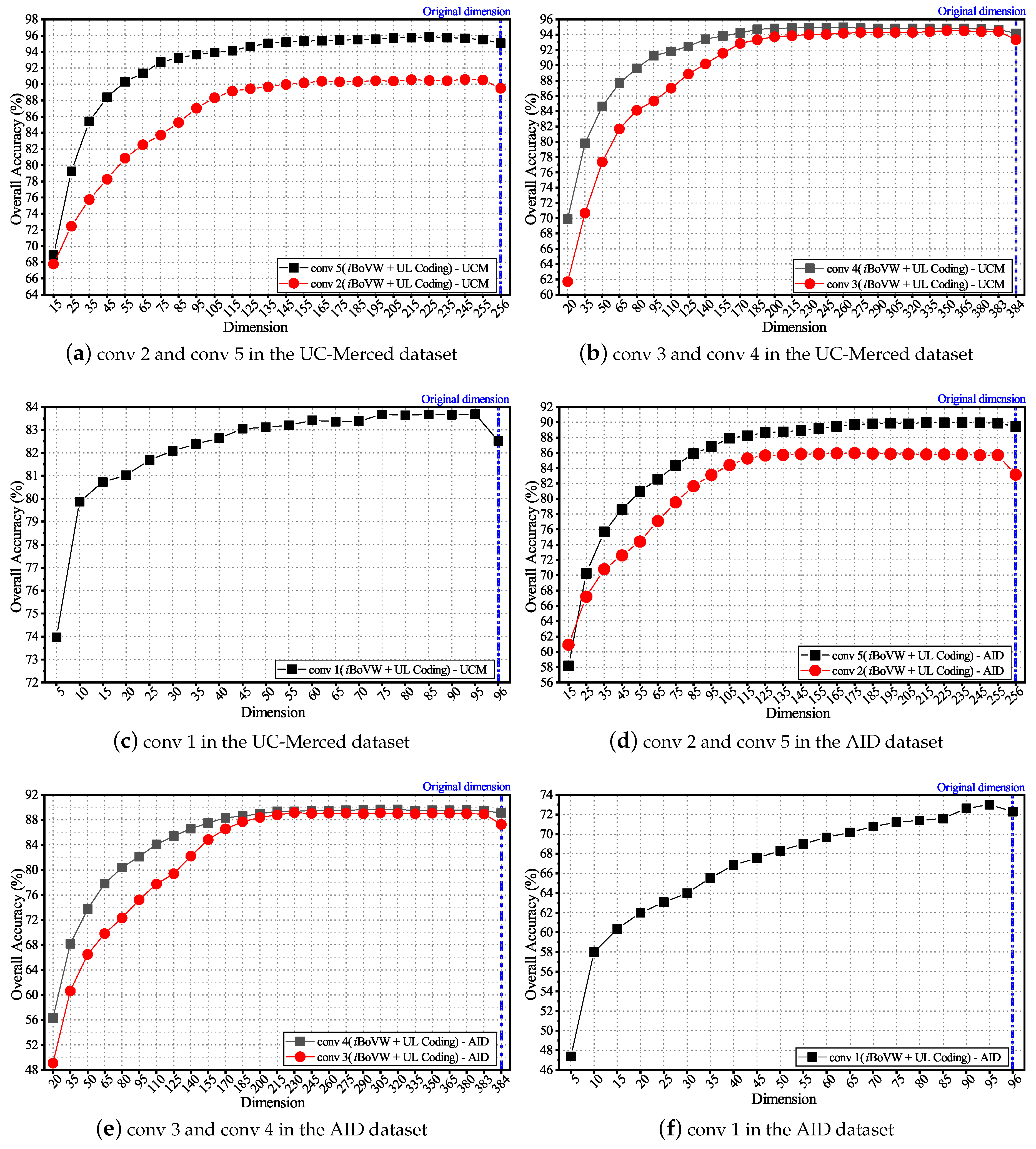
To analyze the influence of the embedding dimension d of deep local features, parameters d were tuned in each convolutional layer with sets of $\{5,10,\dots ,95,96\}$, $\{15,25,\dots ,255,256\}$, $\{20,35,\dots ,383,384\}$, $\{20,35,\dots ,383,384\}$, and $\{15,25,\dots ,255,256\}$, respectively. Figure 7 shows the average OAs under different dimensions; each experiment was repeated 20 times.

According to Figure 7, with the increase in d, the OAs first increase and then remain stable, for the reason that low-dimensional features may lose a lot of useful information. The vertical lines in the figure represent the original dimension of the local deep features on each convolutional layer. It is obvious that the classification accuracy can be improved after employing LPP for dimensionality reduction because LPP can maintain the local geometric structure. To achieve better classification results, parameter d is set to 95, 225, 350, 350, and 235 for each convolutional layer.

4.4. Comparison and Analysis of Proposed Methods

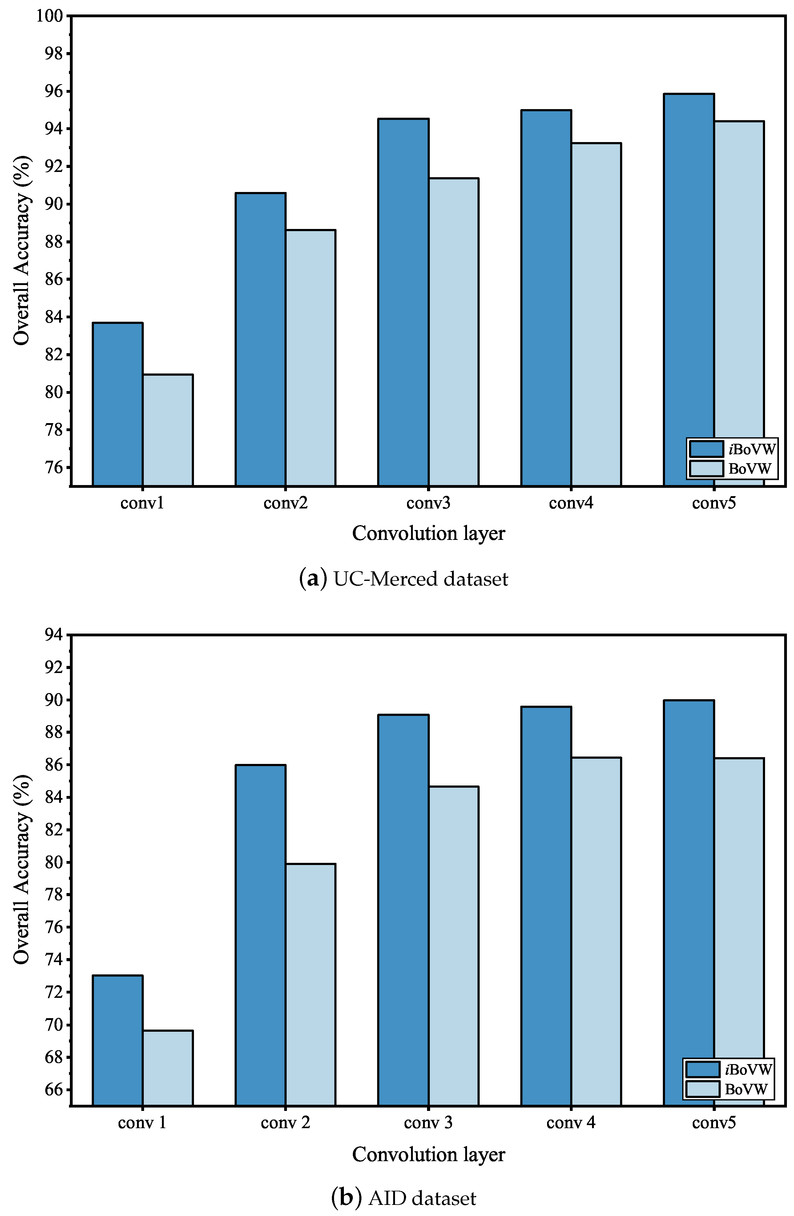
To illustrate the effectiveness of the iBoVW encoding method, OAs obtained from each convolutional layer were compared between the UC-Merced dataset and AID dataset. The value for parameter k for the two dataset was set to 5 and 10, respectively. Figure 8 shows the OAs of different feature encoding methods.

As shown in Figure 8, the proposed iBoVW method achieves a higher OA than the BoVW method in each convolutional layer. The reason is that the traditional BoVW model implements feature coding by using the VQ method, which is a hard assignment method, and VQ assumes that the feature vectors are only related to one visual vocabulary in the dictionary. However, in real applications, the feature vectors are often correlated with multiple clustering centers. Compared with the BoVW method, the proposed iBoVW method adopts non-linear coding to fully consider the correlation between input vectors and multiple clustering centers.

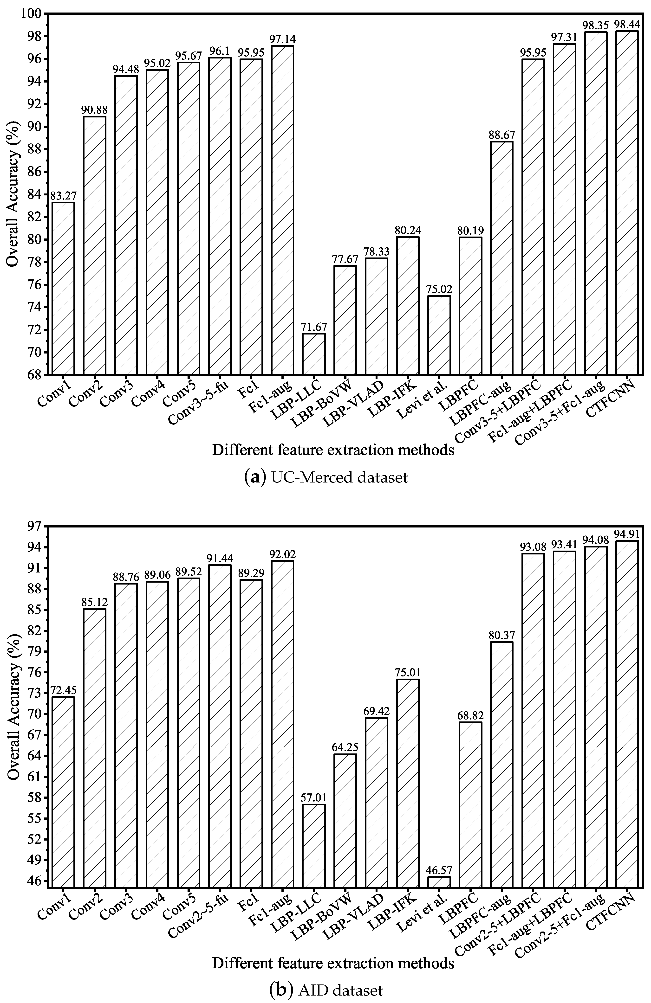
Figure 9 reports the overall accuracy of different CaffeNet-based features. The classification performance of deeper convolutional layers is much better than the lower convolutional layers. Compared with features from single convolutional layer, multilayer feature fusion achieves better results because different convolutional layers contain diverse information, and the ability of discrimination can be improved by fusion. For FC features, data augmentation is helpful to improve classification accuracy. In the UC-Merced dataset, OA was improved from 95.95% to 97.14%. In the AID dataset, it reached 92.02%. Furthermore, it is obvious that our LBP-based CNN method is superior to the mid-level methods, such as LLC, BoVW, VLAD, and IFK. Compared with the method proposed by Levi et al. [68], the proposed pre-processing method is more suitable for LBPFC feature extraction. In summary, the CTFCNN method achieves the highest classification accuracy, which indicates that the strategy of triple-part feature fusion is more effective for scene classification.

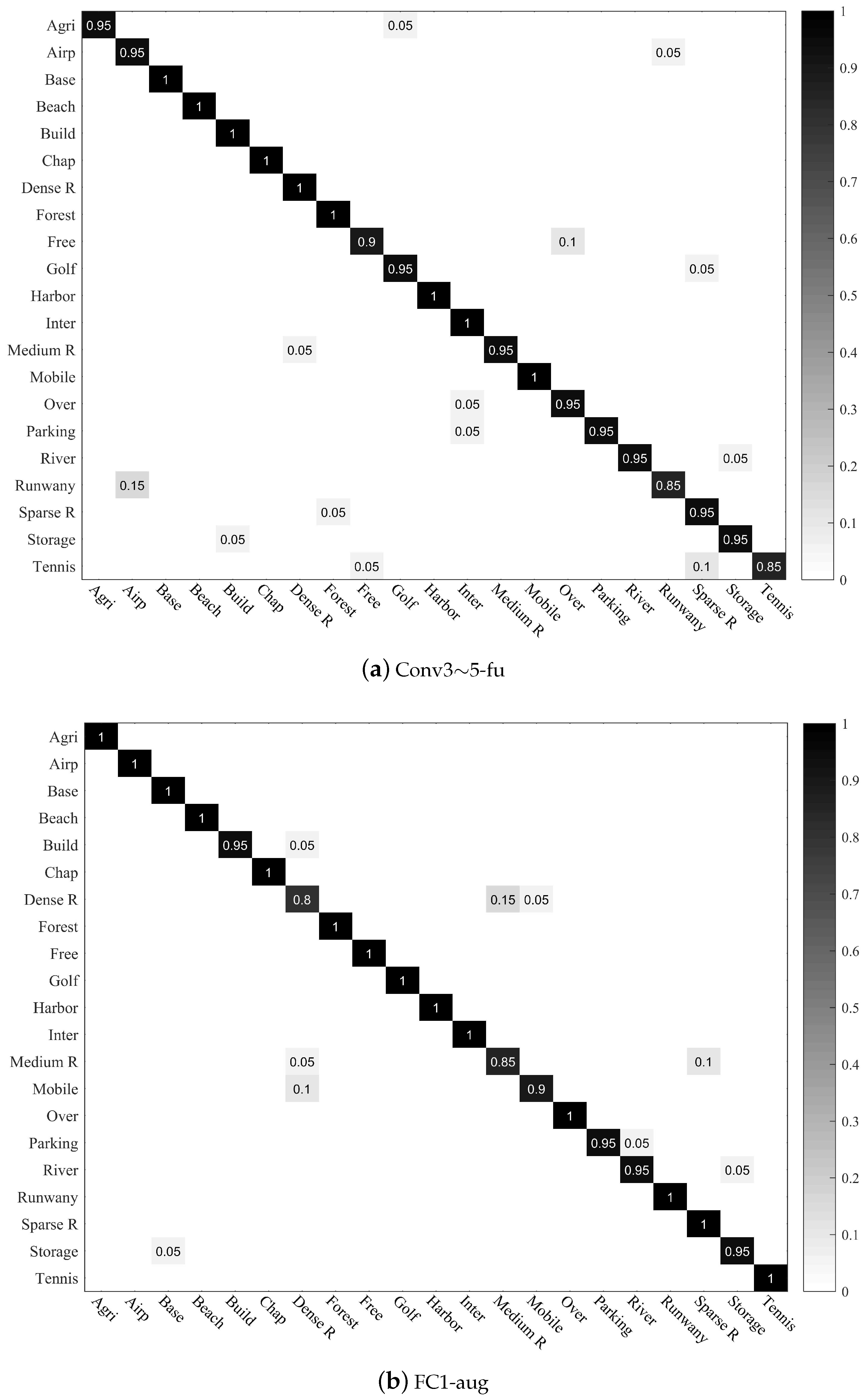
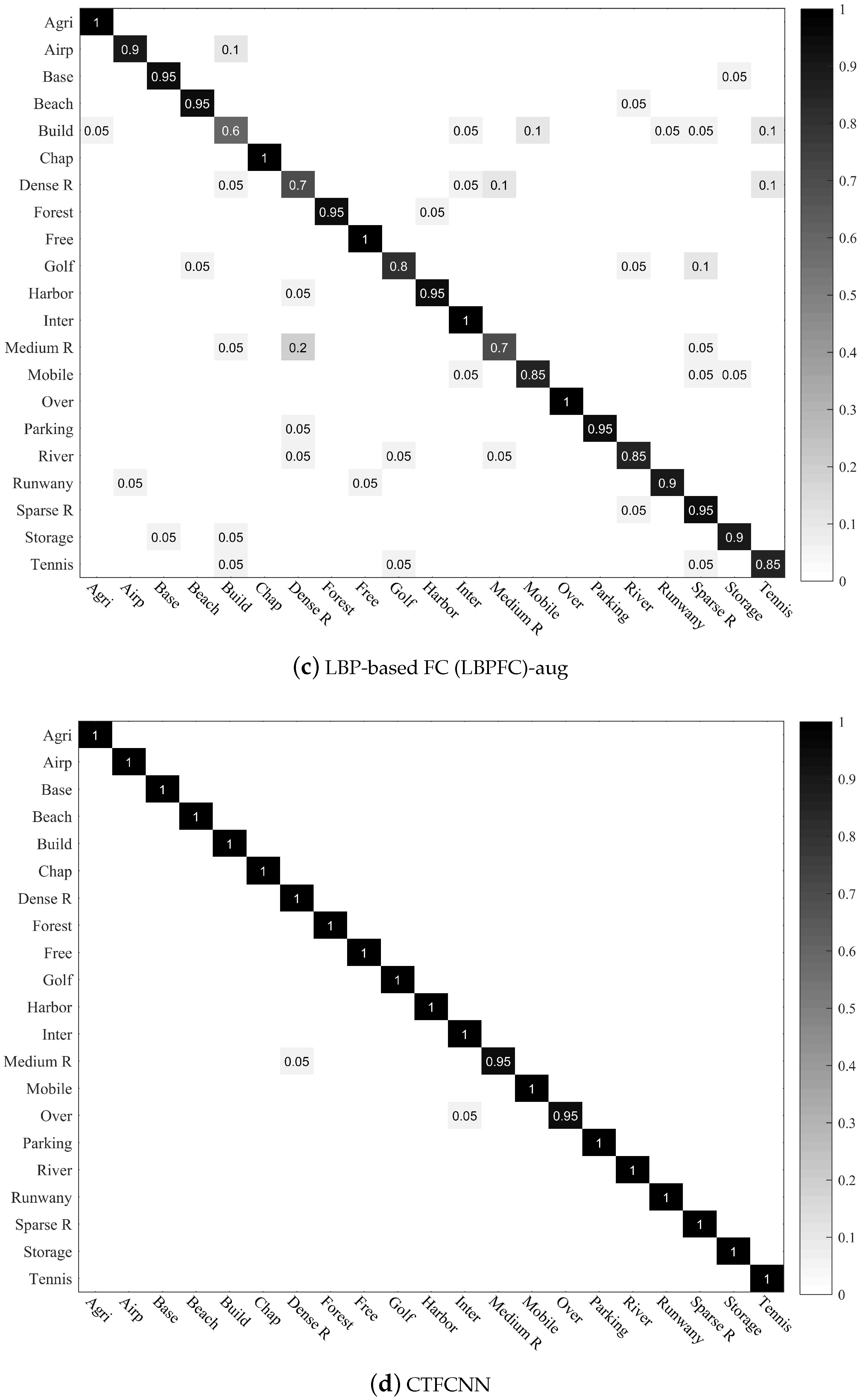
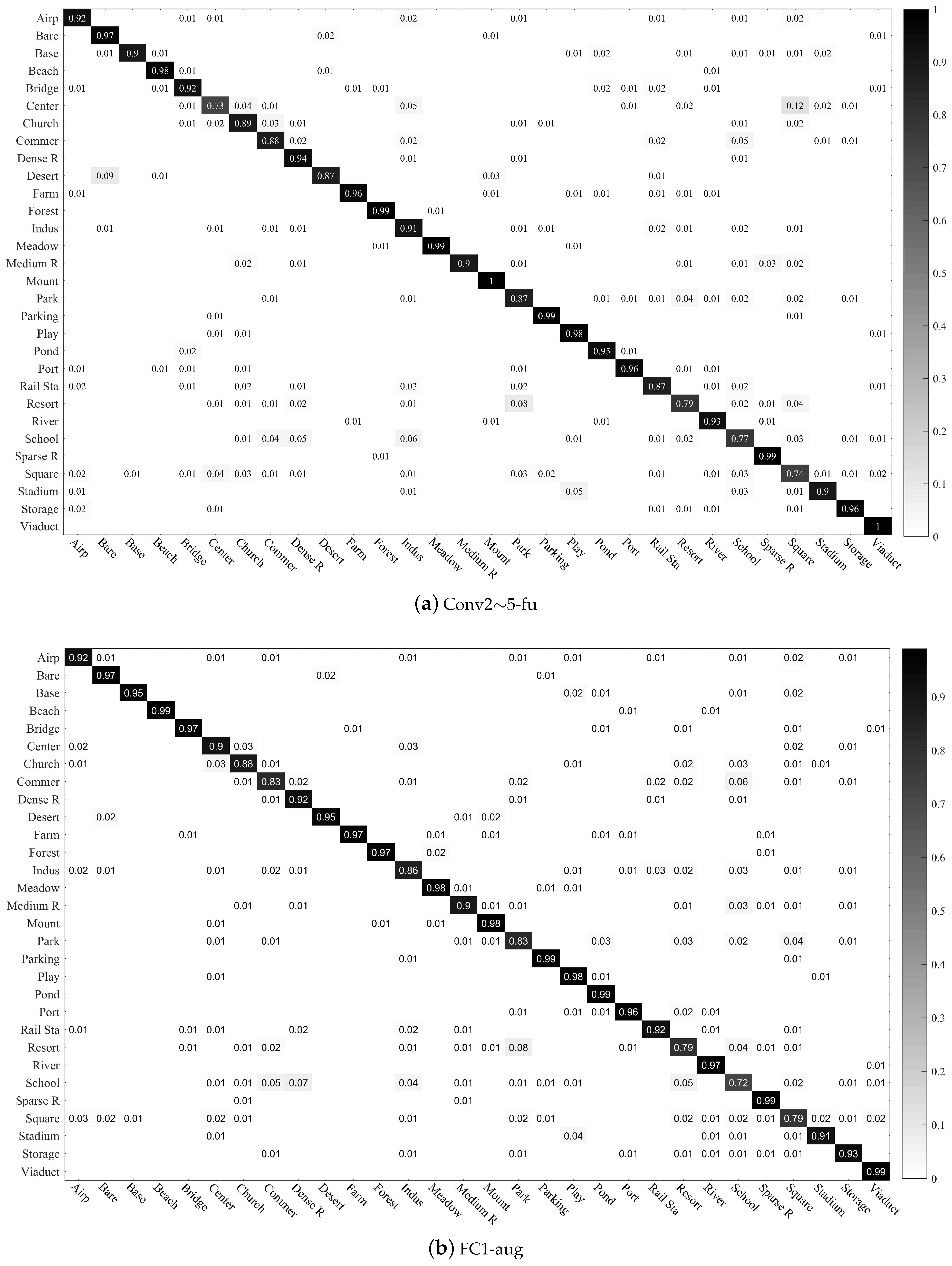
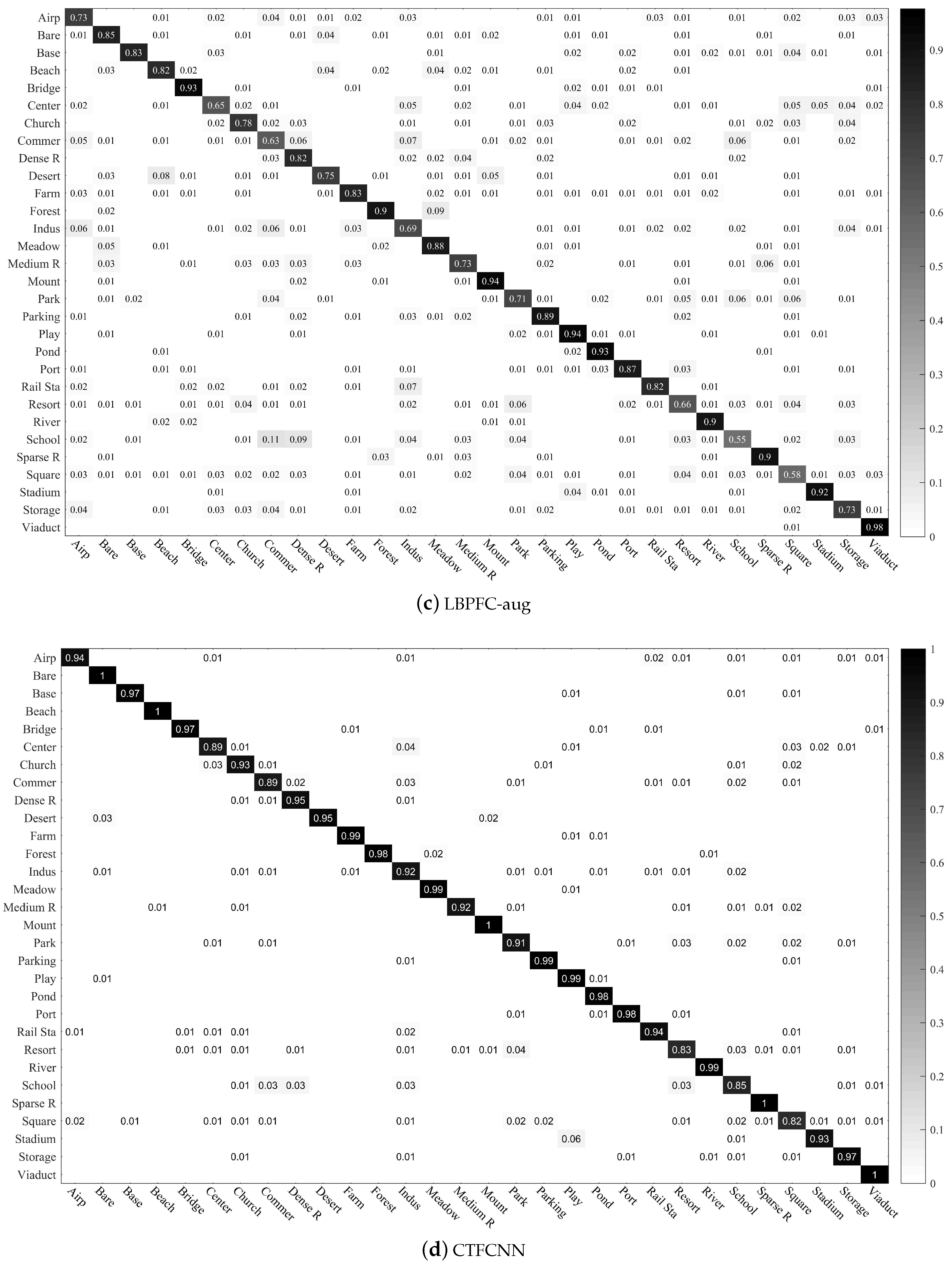
The confusion matrices for the two public datasets are shown in Figure 10 and Figure 11, respectively.

Figure 10 shows the confusion matrices of four methods on the UC-Merced dataset, including single-feature-based methods and the CTFCNN method. It is clear that the CTFCNN method obtains the highest classification performance, and the accuracy of most categories is close to 100%. This shows that the CTFCNN method fully explores the discriminating ability of the pre-trained CNN. Furthermore, our proposed method achieves a relatively good classification accuracy in some high similarity scene categories, such as dense residential (100%), medium residential (95%), and sparse residential (100%).

The confusion matrices for the AID dataset are shown in Figure 11. According to the results, the CTFCNN method is superior to the other methods. In the classes of park (a:0.87, b:0.83, c:0.71, d:0.91), square (a:0.74, b:0.79, c:0.58, d:0.82), school (a:0.77, b:0.72, c:0.55, d:0.85), and resort (a:0.79, b:0.79, c:0.66, d:0.83), the classification performance of the CTFCNN is significantly improved. These semantic classes contain the same types of ground objects (e.g., building, road, and vegetation) and are visually similar, so they are prone to be misclassified. The CTFCNN method still obtains a competitive classification performance, which proves the effectiveness of the feature fusion framework.

4.5. Comparisons with the Most Recent Methods

To comprehensively evaluate the performance of the CTFCNN method, the experimental results of some state-of-the-art methods for two widely-used public datasets are compared in

Table 2. Overall accuracy (mean ± SD) comparison of recent methods under the training ratio of 80% on the UC-Merced dataset.

Method	Published Time	Classification Accuracy (%)
VLAD [69]	2014	92.50
VLAT [69]	2014	94.30
MS-CLBP + FV [70]	2016	93.00 ± 1.20
OverFeat [71]	2017	90.91 ± 1.19
GoogLeNet [22]	2017	94.31 ± 0.89
CaffeNet [22]	2017	95.02 ± 0.81
VGG-VD-16 [22]	2017	95.21 ± 1.20
Bidirectional adaptive feature fusion [72]	2017	95.48
CNN-ELM [73]	2017	95.62 ± 0.32
salM${}^3$LBP-CLM [74]	2017	95.75 ± 0.80
TEX-Net-LF [56]	2017	96.62 ± 0.49
MDDC [75]	2017	96.92 ± 0.57
CaffeNet (conv1 ∼ 5 + fc1) [54]	2017	97.76 ± 0.46
DCA by concatenation [55]	2017	96.90 ± 0.56
DCA by addition [55]	2017	96.90 ± 0.09
DAN (with adaptation) [46]	2017	96.51 ± 0.36
SSF-AlexNet [44]	2018	92.43
Aggregate strategy 1 [17]	2018	97.28
Aggregate strategy 2 [17]	2018	97.40
LASC-CNN (multiscale) [76]	2018	97.14
SPP-net+MKL [77]	2018	96.38 ± 0.92
VGG19 + Hybrid-KCRC (RBF) [52]	2018	96.26
pre-trained ResNet-50 + SRC [53]	2019	96.67
VGG19 + SPM-CRC [51]	2019	96.02
VGG19 + WSPM-CRC [51]	2019	96.14
CTFCNN	Ours	98.44 ± 0.58

Note: The results of the proposed method are marked in bold.

and

Table 3. Overall accuracy (mean ± SD) comparison of recent methods under the training ratio of 50% on the AID dataset.

Method	Published Time	Classification Accuracy (%)
MS-CLBP+FV [70]	2017	86.48 ± 0.27
GoogLeNet [22]	2017	86.39 ± 0.55
VGG-VD-16 [22]	2017	89.64 ± 0.36
CaffeNet [22]	2017	89.53 ± 0.31
DCA with concatenation [55]	2017	89.71 ± 0.33
Fusion by concatenation [55]	2017	91.86 ± 0.28
Fusion by addition [55]	2017	91.87 ± 0.36
Bidirectional adaptive feature fusion [72]	2017	93.56
salM${}^3$LBP-CLM [74]	2017	89.76 ± 0.45
TEX-Net-LF [56]	2017	92.96 ± 0.18
Converted CaffeNet [78]	2018	92.17 ± 0.31
Two-stage deep feature fusion [78]	2018	94.65 ± 0.33
Multilevel fusion [79]	2018	94.17 ± 0.32
ARCNet-VGG16 [4]	2019	93.10 ± 0.55
VGG19 + Hybrid-KCRC (RBF) [52]	2018	91.82
VGG-16-CapsNet [43]	2019	94.74 ± 0.17
VGG19 + SPM-CRC [51]	2019	92.55
VGG19 + WSPM-CRC [51]	2019	92.57
CTFCNN	Ours	94.91 ± 0.24

Note: The results of the proposed method are marked in bold.

, respectively. In these tables, the results of all methods (including the proposed CTFCNN method) were obtained under the same training ratio. In the UC-Merced dataset, the ratio of training–testing was 80% vs. 20%. As for the AID dataset, the ratio was 50% vs. 50%.

From Table 2, we see that the CNN-based methods have achieved more satisfactory results than mid-level methods (i.e., VLAD, VLAT, and MS-CLBP+FV). In [22], three kinds of pre-trained CNN models were employed as feature extractors, and the features from the first fully connected layer were used for classification. In [44,46,51,52,53,71], deep features from pre-trained CNNs were reprocessed to achieved excellent performance. In [73], a deep-learning-based classification method was presented to improve classification performance by combining pre-trained CNNs and extreme learning machine (ELM). In [56,72,74], deep features and hand-crafted features were combined to get a discriminative scene presentation. In [54,55], multilayer features based on a convolutional neural network were fused to get better results. In addition, the work reported in [75,76] attempted to adopt a multiscale feature fusion strategy. In contrast, our proposed method provides an improvement over recent CNN-based methods and focuses on combing triple-part features of a CNN model for classification. On the UC-Merced dataset, the highest classification accuracy of the CTFCNN was 98.44%.

Compared with the UC-Merced dataset, the AID dataset is available later (in 2017), and it is larger scale dataset. However, the CTFCNN method achieved excellent classification results (94.91%) on the AID dataset. As can be seen from Table 3, the performance of our proposed method is better than some state-of-the-art methods, which are based on pre-trained CNNs. In [78,79], a two-stage deep feature fusion method and multilevel fusion methods achieve satisfactory results. The reason is that they adopt multiple types of CNN models, including CaffeNet and VGG-VD-16, while our method only employs one type of CNN model. The classification result in [43] is good, because CNN and CapsNet are integrated, and feature maps from a pre-tained VGG-16 are fed into CapsNet and participated in fine-tuning. The above analysis indicates that the proposed CTFCNN method can effectively extract the discriminating features of scenes to achieve better classification.

5. Conclusions

In this paper, we proposed a CTFCNN framework to fully exploit the discriminant ability of a pre-trained CaffeNet. In this framework, CaffeNet is employed as a feature extractor to get multilayer convolutional features, features from the fully connected layer, and LBP-based FC features. Then, the iBoVW method is developed to process the convolutional features, which employs LPP and a nonlinear coding method. For the LBP-based FC features, a new solution is proposed to integrate texture images and pre-trained CNN models. Finally, three features are combined by weighted concatenation. As a result, the proposed framework can effectively achieve the representations of HSRRS images and improve the performance of scene classification. Experimental results on two public datasets (UC-Merced and AID) show that the CTFCNN method obtains much better results than some state-of-the-art methods in terms of overall accuracy, and the highest OAs achieved were 98.44% and 94.91%, respectively. In the future, we will incorporate fine-tuning techniques and focus on combing features from regions of interest (ROIs) to further improve the classification performance.

References

- Cheng, G.; Han, J.W.; Lu, X.Q. Remote sensing image scene classification: Benchmark and state of the art. Proc. IEEE 2017, 105, 1865–1883. [Google Scholar] [CrossRef]
- Zhou, W.X.; Newsam, S.; Li, C.M.; Shao, Z.F. PatternNet: A benchmark dataset for performance evaluation of remote sensing image retrieval. ISPRS J. Photogramm. Remote Sens. 2018, 145, 197–209. [Google Scholar] [CrossRef] [Green Version]
- Zhang, F.; Du, B.; Zhang, L.P. Scene Classification via a Gradient Boosting Random Convolutional Network Framework. IEEE Trans. Geosci. Remote Sens. 2016, 54, 1793–1802. [Google Scholar] [CrossRef]
- Wang, Q.; Liu, S.T.; Chanussot, J.; Li, X.L. Scene Classification with Recurrent Attention of VHR Remote Sensing Images. IEEE Trans. Geosci. Remote Sens. 2019, 57, 1155–1167. [Google Scholar] [CrossRef]
- Pham, M.T.; Mercier, G.; Regniers, O.; Michel, J. Texture Retrieval from VHR Optical Remote Sensed Images Using the Local Extrema Descriptor with Application to Vineyard Parcel Detection. Remote Sens. 2016, 8, 368. [Google Scholar] [CrossRef]
- Napoletano, P. Visual descriptors for content-based retrieval of remote-sensing images. Int. J. Remote Sens. 2018, 39, 1343–1376. [Google Scholar] [CrossRef]
- Yang, Y.; Newsam, S. Geographic image retrieval using local invariant features. IEEE Trans. Geosci. Remote Sens. 2013, 51, 818–832. [Google Scholar] [CrossRef]
- Sun, W.W.; Wang, R.S. Fully Convolutional Networks for Semantic Segmentation of Very High Resolution Remotely Sensed Images Combined With DSM. IEEE Geosci. Remote Sens. Lett. 2018, 15, 474–478. [Google Scholar] [CrossRef]
- Hu, T.Y.; Yang, J.; Li, X.C.; Gong, P. Mapping Urban Land Use by Using Landsat Images and Open Social Data. Remote Sens. 2016, 8, 151. [Google Scholar] [CrossRef]
- Huang, B.; Zhao, B.; Song, Y.M. Urban land-use mapping using a deep convolutional neural network with high spatial resolution multispectral remote sensing imagery. Remote Sens. Environ. 2018, 214, 73–86. [Google Scholar] [CrossRef]
- Zhong, Y.F.; Han, X.B.; Zhang, L.P. Multi-class geospatial object detection based on a position-sensitive balancing framework for high spatial resolution remote sensing imagery. ISPRS J. Photogramm. Remote Sens. 2018, 138, 281–294. [Google Scholar] [CrossRef]
- Deng, Z.P.; Sun, H.; Zhou, S.L.; Zhao, J.P.; Lei, L.; Zou, H.X. Multi-scale object detection in remote sensing imagery with convolutional neural networks. ISPRS J. Photogramm. Remote Sens. 2018, 145, 3–22. [Google Scholar] [CrossRef]
- Cheng, G.; Han, J.W.; Zhou, P.C.; Guo, L. Multi-class geospatial object detection and geographic image classification based on collection of part detectors. ISPRS J. Photogramm. Remote Sens. 2014, 98, 119–132. [Google Scholar] [CrossRef]
- Manfreda, S.; McCabe, M.F.; Miller, P.E.; Lucas, R.; Pajuelo Madrigal, V.; Mallinis, G.; Ben Dor, E.; Helman, D.; Estes, L.; Ciraolo, G.; et al. On the use of unmanned aerial systems for environmental monitoring. Remote Sens. 2018, 10, 641. [Google Scholar] [CrossRef]
- Khan, N.; Chaudhuri, U.; Banerjee, B.; Chaudhuri, S. Graph convolutional network for multi-label VHR remote sensing scene recognition. Neurocomputing 2019, 357, 36–46. [Google Scholar] [CrossRef]
- He, N.J.; Fang, L.Y.; Li, S.T.; Plaza, A.; Plaza, J. Remote Sensing Scene Classification Using Multilayer Stacked Covariance Pooling. IEEE Trans. Geosci. Remote Sens. 2018, 51, 6899–6910. [Google Scholar] [CrossRef]
- Liu, N.; Wan, L.H.; Zhang, Y.; Zhou, T.; Huo, H.; Fang, T. Exploiting Convolutional Neural Networks with Deeply Local Description for Remote Sensing Image Classification. IEEE Access 2018, 6, 11215–11228. [Google Scholar] [CrossRef]
- Jin, P.; Xia, G.S.; Hu, F.; Lu, Q.K.; Zhang, L.P. AID++: An Updated Version of AID on Scene Classification. In Proceedings of the 2018 IEEE International Geoscience and Remote Sensing Symposium (IGARSS), Valencia, Spain, 22–27 July 2018; pp. 4721–4724. [Google Scholar]
- Hu, F.; Xia, G.S.; Yang, W.; Zhang, L.P. Recent advances and opportunities in scene classification of aerial images with deep models. In Proceedings of the 2018 IEEE International Geoscience and Remote Sensing Symposium (IGARSS), Valencia, Spain, 22–27 July 2018; pp. 4371–4374. [Google Scholar]
- Romero, A.; Gatta, C.; Camps-Valls, G. Unsupervised Deep Feature Extraction for Remote Sensing Image Classification. IEEE Trans. Geosci. Remote Sens. 2016, 54, 1349–1362. [Google Scholar] [CrossRef]
- Yu, Y.L.; Liu, F.X. Dense connectivity based two-stream deep feature fusion framework for aerial scene classification. Remote Sens. 2018, 10, 1158. [Google Scholar] [CrossRef]
- Xia, G.S.; Hu, J.; Hu, F.; Shi, B.; Bai, X.; Zhong, Y.; Zhang, L.; Lu, X. AID: A benchmark data set for performance evaluation of aerial scene classification. IEEE Trans. Geosci. Remote Sens. 2017, 55, 3965–3981. [Google Scholar] [CrossRef]
- Luo, B.; Jiang, S.J.; Zhang, L.P. Indexing of remote sensing images with different resolutions by multiple features. IEEE J. Sel. Top. Appl. Earth Obs. Remote Sens. 2013, 6, 1899–1912. [Google Scholar] [CrossRef]
- Yang, Y.; Newsam, S. Comparing SIFT descriptors and Gabor texture features for classification of remote sensed imagery. In Proceedings of the 15th IEEE International Conference on Image Processing (ICIP 2008), San Diego, CA, USA, 12–15 October 2008; pp. 1852–1855. [Google Scholar]
- Yang, Y.; Newsam, S. Bag-of-visual-words and spatial extensions for land-use classification. In Proceedings of the 18th SIGSPATIAL International Conference on Advances in Geographic Information Systems, San Jose, CA, USA, 2–5 November 2010; pp. 270–279. [Google Scholar]
- Zhu, Q.Q.; Zhong, Y.F.; Zhao, B.; Xia, G.S.; Zhang, L.P. Bag-of-visual-words scene classifier with local and global features for high spatial resolution remote sensing imagery. IEEE Geosci. Remote Sens. Lett. 2016, 13, 747–751. [Google Scholar] [CrossRef]
- Zhao, L.J.; Tang, P.; Huo, L.Z. Land-use scene classification using a concentric circle-structured multiscale bag-of-visual-words model. IEEE J. Sel. Top. Appl. Earth Obs. Remote Sens. 2014, 7, 4620–4631. [Google Scholar] [CrossRef]
- Wu, H.; Liu, B.Z.; Su, W.H.; Zhang, W.; Sun, J.G. Hierarchical coding vectors for scene level land-use classification. Remote Sens. 2016, 8, 436. [Google Scholar] [CrossRef]
- Qi, K.L.; Wu, H.Y.; Shen, C.; Gong, J.Y. Land-Use Scene Classification in High-Resolution Remote Sensing Images Using Improved Correlatons. Remote Sens. Lett. 2015, 12, 2403–2407. [Google Scholar]
- Perronnin, F.; Sánchez, J.; Mensink, T. Improving the Fisher Kernel for Large-Scale Image Classification. In Proceedings of the European Conference on Computer Vision, Crete, Greece, 5–11 September 2010; pp. 143–156. [Google Scholar]
- Wang, G.L.; Fan, B.; Xiang, S.M.; Pan, C.H. Aggregating rich hierarchical features for scene classification in remote sensing imagery. IEEE J. Sel. Top. Appl. Earth Obs. Remote Sens. 2017, 10, 4104–4115. [Google Scholar] [CrossRef]
- Lu, X.Q.; Zheng, X.T.; Yuan, Y. Remote Sensing Scene Classification by Unsupervised Representation Learning. IEEE Trans. Geosci. Remote Sens. 2017, 55, 5148–5157. [Google Scholar] [CrossRef]
- Zou, J.; Li, W.; Chen, C.; Du, Q. Scene classification using local and global features with collaborative representation fusion. Inf. Sci. 2018, 348, 209–226. [Google Scholar] [CrossRef]
- Fernandez-Beltran, R.; Haut, J.M.; Paoletti, M.E.; Plaza, J.; Plaza, A.; Pla, F. Remote Sensing Image Fusion Using Hierarchical Multimodal Probabilistic Latent Semantic Analysis. IEEE J. Sel. Top. Appl. Earth Obs. Remote Sens. 2018, 11, 4982–4993. [Google Scholar] [CrossRef]
- Zhong, Y.F.; Zhu, Q.Q.; Zhang, L.P. Scene Classification Based on the Multifeature Fusion Probabilistic Topic Model for High Spatial Resolution Remote Sensing Imagery. IEEE Trans. Geosci. Remote Sens. 2015, 53, 6207–6222. [Google Scholar] [CrossRef]
- Ball, J.E.; Anderson, D.T.; Chan, C.S. Comprehensive survey of deep learning in remote sensing: Theories, tools, and challenges for the community. J. Appl. Remote Sens. 2017, 11, 042609. [Google Scholar] [CrossRef]
- Zhu, X.X.; Tuia, D.; Mou, L.; Xia, G.S.; Zhang, L.; Xu, F.; Fraundorfer, F. Deep Learning in Remote Sensing: A Comprehensive Review and List of Resources. IEEE Geosci. Remote Sens. Mag. 2017, 5, 8–36. [Google Scholar] [CrossRef] [Green Version]
- Yang, H.P.; Yu, B.; Luo, J.C.; Chen, F. Semantic segmentation of high spatial resolution images with deep neural networks. GISci. Remote Sens. 2019, 56, 749–768. [Google Scholar] [CrossRef]
- Wang, Q.; Yuan, Z.H.; Du, Q.; Li, X.L. GETNET: A General End-to-End 2-D CNN Framework for Hyperspectral Image Change Detection. IEEE Trans. Geosci. Remote Sens. 2019, 57, 3–13. [Google Scholar] [CrossRef]
- Yuan, Q.Q.; Zhang, Q.; Li, J.; Shen, H.F.; Zhang, L.P. Hyperspectral Image Denoising Employing a Spatial-Spectral Deep Residual Convolutional Neural Network. IEEE Trans. Geosci. Remote Sens. 2019, 57, 1205–1218. [Google Scholar] [CrossRef]
- Jian, L.; Gao, F.H.; Ren, P.; Song, Y.Q.; Luo, S.H. A Noise-Resilient Online Learning Algorithm for Scene Classification. Remote Sens. 2018, 10, 1836. [Google Scholar] [CrossRef]
- Scott, G.J.; Hagan, K.C.; Marcum, R.A.; Hurt, J.A.; Anderson, D.T.; Davis, C.H. Enhanced Fusion of Deep Neural Networks for Classification of Benchmark High-Resolution Image Data Sets. IEEE Geosci. Remote Sens. Lett. 2018, 15, 1451–1455. [Google Scholar] [CrossRef]
- Zhang, W.; Tang, P.; Zhao, L.J. Remote Sensing Image Scene Classification Using CNN-CapsNet. Remote Sens. 2019, 11, 494. [Google Scholar] [CrossRef]
- Chen, J.B.; Wang, C.Y.; Ma, Z.; Chen, J.S.; He, D.X.; Ackland, S. Remote Sensing Scene Classification Based on Convolutional Neural Networks Pre-Trained Using Attention-Guided Sparse Filters. Remote Sens. 2018, 10, 290. [Google Scholar] [CrossRef]
- Liu, Y.S.; Suen, C.Y.; Liu, Y.B.; Ding, L.W. Scene Classification Using Hierarchical Wasserstein CNN. IEEE Trans. Geosci. Remote Sens. 2019, 57, 2494–2509. [Google Scholar] [CrossRef]
- Othman, E.; Bazi, Y.; Melgani, F.; Alhichri, H.; Alajlan, N.; Zuair, M. Domain Adaptation Network for Cross-Scene Classification. IEEE Trans. Geosci. Remote Sens. 2017, 55, 4441–4456. [Google Scholar] [CrossRef]
- Liu, Y.S.; Huang, C. Scene Classification via Triplet Networks. IEEE J. Sel. Top. Appl. Earth Obs. Remote Sens. 2018, 11, 220–237. [Google Scholar] [CrossRef]
- Zou, Q.; Ni, L.H.; Zhang, T.; Wang, Q. Deep Learning Based Feature Selection for Remote Sensing Scene Classification. IEEE Geosci. Remote Sens. Lett. 2015, 12, 2321–2325. [Google Scholar] [CrossRef]
- Penatti, O.A.; Nogueira, K.; dos Santos, J.A. Do deep features generalize from everyday objects to remote sensing and aerial scenes domains? In Proceedings of the 2015 IEEE Conference on Computer Vision and Pattern Recognition Workshops (CVPRW), Boston, MA, USA, 7 June 2015; pp. 44–51. [Google Scholar]
- Hu, F.; Xia, G.S.; Hu, J.W.; Zhang, L.P. Transferring Deep Convolutional Neural Networks for the Scene Classification of High-Resolution Remote Sensing Imagery. Remote Sens. 2015, 7, 14680–14707. [Google Scholar] [CrossRef] [Green Version]
- Liu, B.D.; Jie, M.; Xie, W.Y.; Shao, S.; Li, Y.; Wang, Y.J. Weighted Spatial Pyramid Matching Collaborative Representation for Remote-Sensing-Image Scene Classification. Remote Sens. 2019, 11, 518. [Google Scholar] [CrossRef]
- Liu, B.D.; Xie, W.Y.; Meng, J.; Li, Y.; Wang, Y.J. Hybrid collaborative representation for remote-sensing image scene classification. Remote Sens. 2018, 10, 1934. [Google Scholar] [CrossRef]
- Flores, E.; Zortea, M.; Scharcanski, J. Dictionaries of deep features for land-use scene classification of very high spatial resolution images. Pattern Recognit. 2019, 89, 32–44. [Google Scholar] [CrossRef]
- Li, E.Z.; Xia, J.S.; Du, P.J.; Lin, C.; Samat, A. Integrating Multilayer Features of Convolutional Neural Networks for Remote Sensing Scene Classification. IEEE Trans. Geosci. Remote Sens. 2017, 55, 5653–5665. [Google Scholar] [CrossRef]
- Chaib, S.; Liu, H.; Gu, Y.F.; Yao, H.X. Deep Feature Fusion for VHR remote sensing scene classification. IEEE Trans. Geosci. Remote Sens. 2017, 55, 4775–4784. [Google Scholar] [CrossRef]
- Anwer, R.M.; Khan, F.S.; van deWeijer, J.; Monlinier, M.; Laaksonen, J. Binary patterns encoded convolutional neural networks for texture recognition and remote sensing scene classification. ISPRS J. Photogramm. Remote Sens. 2018, 138, 74–85. [Google Scholar] [CrossRef] [Green Version]
- Gu, J.X.; Wang, Z.H.; Kuen, J.; Ma, L.Y.; Shahroudy, A.; Shuai, B.; Liu, T.; Wang, X.X.; Wang, G.; Cai, J.F.; et al. Recent Advances in Convolutional Neural Networks. Pattern Recognit. 2018, 77, 354–377. [Google Scholar] [CrossRef]
- Yang, X.; He, H.B.; Wei, Q.L.; Luo, B. Reinforcement learning for robust adaptive control of partially unknown nonlinear systems subject to unmatched uncertainties. Inf. Sci. 2018, 463, 307–322. [Google Scholar] [CrossRef]
- Jia, Y.; Shelhamer, E.; Donahue, J.; Karayev, S.; Long, J.; Girshick, R.; Guadarrama, S.; Darrell, T. Caffe: Convolutional architecture for fast feature embedding. In Proceedings of the 22nd ACM International Conference on Multimedia, Orlando, FL, USA, 3–7 November 2014; pp. 675–678. [Google Scholar]
- Lima, E.; Sun, X.; Dong, J.Y.; Wang, H.; Yang, Y.T.; Liu, L.P. Learning and Transferring Convolutional Neural Network Knowledge to Ocean Front Recognition. IEEE Geosci. Remote Sens. Lett. 2017, 14, 354–358. [Google Scholar] [CrossRef]
- Zhao, F.A.; Mu, X.D.; Yang, Z.; Yi, Z.X. Hierarchical feature coding model for high-resolution satellite scene classification. J. Appl. Remote Sens. 2019, 13, 016520. [Google Scholar] [CrossRef]
- Ahonen, T.; Hadid, A.; Pietikainen, M. Face description with local binary patterns: Application to face recognition. IEEE Trans. Pattern Anal. Mach. Intell. 2006, 28, 2037–2041. [Google Scholar] [CrossRef] [PubMed]
- Li, W.; Chen, C.; Su, H.J.; Du, Q. Local Binary Patterns and Extreme Learning Machine for Hyperspectral Imagery Classification. IEEE Trans. Geosci. Remote Sens. 2015, 53, 3681–3693. [Google Scholar] [CrossRef]
- Huang, H.; Li, Z.Y.; Pan, Y.S. Multi-Feature Manifold Discriminant Analysis for Hyperspectral Image Classification. Remote Sens. 2019, 11, 651. [Google Scholar] [CrossRef]
- Yang, F.; Xu, Q.Z.; Li, B. Ship Detection From Optical Satellite Images Based on Saliency Segmentation and Structure-LBP Feature. IEEE Geosci. Remote Sens. Lett. 2017, 14, 602–606. [Google Scholar] [CrossRef]
- Fan, R.E.; Chang, K.W.; Hsieh, C.J.; Wang, X.R.; Lin, C.J. LIBLINEAR: A library for large linear classification. J. Mach. Learn. Res. 2008, 9, 1871–1874. [Google Scholar]
- Vedaldi, A.; Lenc, K. Matconvnet: Convolutional neural networks for matlab. In Proceedings of the 23rd ACM International Conference on Multimedia, Brisbane, Australia, 26–30 October 2015; ACM: New York, NY, USA, 2015; pp. 689–692. [Google Scholar]
- Levi, G.; Hassner, T. Emotion recognition in the wild via convolutional neural networks and mapped binary patterns. In Proceedings of the 2015 ACM on International Conference on Multimodal Interaction, Seattle, WA, USA, 9–13 Novmber 2015; pp. 503–510. [Google Scholar]
- Negrel, R.; Picard, D.; Gosselin, P.H. Evaluation of second-order visual features for land-use classification. In Proceedings of the 2014 12th International Workshop on Content-Based Multimedia Indexing (CBMI 2014), Klagenfurt, Austria, 18–20 June 2014; pp. 1–5. [Google Scholar]
- Huang, L.H.; Chen, C.; Li, W.; Du, Q. Remote sensing image scene classification using multi-scale completed local binary patterns and fisher vectors. Remote Sens. 2016, 8, 483. [Google Scholar] [CrossRef]
- Nogueira, K.; Penatti, O.A.B.; dos Santos, J.A. Towards better exploiting convolutional neural networks for remote sensing scene classification. Pattern Recognit. 2017, 61, 539–556. [Google Scholar] [CrossRef] [Green Version]
- Ji, W.J.; Li, X.L.; Lu, X.Q. Bidirectional Adaptive Feature Fusion for Remote Sensing Scene Classification. In Proceedings of the Second CCF Chinese Conference (CCCV 2017), Tianjin, China, 11–14 October 2017; pp. 486–497. [Google Scholar]
- Weng, Q.; Mao, Z.Y.; Lin, J.W.; Guo, W.Z. Land-use classification via extreme learning classifier based on deep convolutional features. IEEE Geosci. Remote Sens. Lett. 2017, 14, 704–708. [Google Scholar] [CrossRef]
- Bian, X.Y.; Chen, C.; Tian, L.; Du, Q. Fusing local and global features for high-resolution scene classification. IEEE J. Sel. Top. Appl. Earth Obs. Remote Sens. 2017, 10, 2889–2901. [Google Scholar] [CrossRef]
- Qi, K.L.; Yang, C.; Guan, Q.F.; Wu, H.Y.; Gong, J.Y. A Multiscale Deeply Described Correlatons-Based Model for Land-Use Scene Classification. Remote Sens. 2017, 9, 917. [Google Scholar] [CrossRef]
- Yuan, B.H.; Li, S.J.; Li, N. Multiscale deep features learning for land-use scene recognition. J. Appl. Remote Sens. 2018, 12, 015010. [Google Scholar] [CrossRef]
- Liu, Q.S.; Hang, R.L.; Song, H.H.; Li, Z. Learning Multiscale Deep Features for High-Resolution Satellite Image Scene Classification. IEEE Trans. Geosci. Remote Sens. 2018, 56, 117–126. [Google Scholar] [CrossRef]
- Liu, Y.S.; Liu, Y.B.; Ding, L.W. Scene Classification Based on Two-Stage Deep Feature Fusion. IEEE Geosci. Remote Sens. Lett. 2018, 15, 183–186. [Google Scholar] [CrossRef]
- Yu, Y.; Liu, F. Aerial Scene Classification via Multilevel Fusion Based on Deep Convolutional Neural Networks. IEEE Geosci. Remote Sens. Lett. 2018, 15, 287–291. [Google Scholar] [CrossRef]
Figure 1.
Architecture of CaffeNet.
Figure 2.
The principle of local binary pattern (LBP) descriptors. HSRRS—high spatial resolution remote sensing.
Figure 3.
Framework of the proposed CTFCNN method. HSRRS—high spatial resolution remote sensing; CNN—convolutional neural network; FC—fully connected; PCA—principal component analysis; SVM—support vector machine.
Figure 4.
The procedures of deep local feature extraction and improved bag-of-view-word (iBoVW) encoding.
Figure 5.
Example images for two remote sensing image datasets.
Figure 6.
OAs with respect to different sizes of visual vocabulary on two public datasets.
Figure 7.
Overall accuracy (OA) with respect to different sizes of visual vocabulary on two public datasets.
Figure 8.
Figure 9.
OAs of different feature extraction methods on two public datasets.
Figure 10.
Confusion matrices of CTFCNN for the UC-Merced dataset. In confusion matrices, each row denotes the instances in actual category, and each column of the matrix denotes the instances in a predicted category. Blank positions indicate that the value is 0, and the diagonal data indicates the accuracy of each class.
Figure 11.
Confusion matrices of CTFCNN for the AID dataset.