Evaluation of Leaf N Concentration in Winter Wheat Based on Discrete Wavelet Transform Analysis

Abstract

Leaf nitrogen concentration (LNC) is an important indicator for accurate diagnosis and quantitative evaluation of plant growth status. The objective was to apply a discrete wavelet transform (DWT) analysis in winter wheat for the estimation of LNC based on visible and near-infrared (400–1350 nm) canopy reflectance spectra. In this paper, in situ LNC data and ground-based hyperspectral canopy reflectance was measured over three years at different sites during the tillering, jointing, booting and filling stages of winter wheat. The DWT analysis was conducted on canopy original spectrum, log-transformed spectrum, first derivative spectrum and continuum removal spectrum, respectively, to obtain approximation coefficients, detail coefficients and energy values to characterize canopy spectra. The quantitative relationships between LNC and characteristic parameters were investigated and compared with models established by sensitive band reflectance and typical spectral indices. The results showed combining log-transformed spectrum and a sym8 wavelet function with partial least squares regression (PLS) based on the approximation coefficients at decomposition level 4 most accurately predicted LNC. This approach could explain 11% more variability in LNC than the best spectral index mSR₇₀₅ alone, and was more stable in estimating LNC than models based on random forest regression (RF). The results indicated that narrowband reflectance spectroscopy (450–1350 nm) combined with DWT analysis and PLS regression was a promising method for rapid and nondestructive estimation of LNC for winter wheat across a range in growth stages.

1. Introduction

Nitrogen (N) is one of the essential elements in plants. N deficiency seriously affects the photosynthesis process and physiological metabolism and results in poor wheat grain yield and quality [1,2]. Excessive N over fertilization not only fails to increase crop yield, but also causes the unnecessary purchase of fertilizer and results in environmental pollution [3,4]. Knowledge of in-season plant N status is the key to guiding N fertilization for farmers. Leaf nitrogen concentration (LNC) is an important indicator of N nutrition in crops and is desired to be obtained by a rapid, non-destructive method [5]. Hyperspectral remote sensing captures continuous and subtle spectral absorption features of crop canopy from narrow bands, which has been widely applied to differentiate and quantify the biophysical and biochemical parameters of agricultural crops [6]. Absorption characteristics of N itself are quite weak and often are expressed by amino acid absorption characteristics in protein. The sensitive absorption wavelength of N lies in short-wave-infrared (SWIR), which is easily obscured by water-vapor absorption characteristics [7,8]. Visible spectrum (VIS) and near-infrared (NIR) band reflectance are often used to estimate LNC indirectly due to the strong positive correlation with leaf chlorophyll content and pronounced sensitivity to canopy structures [9,10,11,12].

Among the estimating approaches, linear or non-linear regression models are typically analyzed based on individual input variable of sensitive waveband reflectance. However, the canopy reflectance spectra and sensitive wavebands of LNC are easily and strongly influenced by the soil background, vegetation canopy geometry and atmospheric conditions [13]. Spectral transformation techniques such as first derivative transformation, continuum removal and log-transformation processing techniques are applied to reduce the effects of the surroundings and to enhance the spectral sensitivity to crop N content [11,14,15]. However, it remains to be discussed about which spectral transformation is more effective in canopy N evaluation. Meanwhile, a number of spectral indices sensitive to chlorophyll and canopy structures with robustness have been developed to minimize spectral noise and to estimate N-related indicators [16,17,18]. These include the modified normalized difference (mND₇₀₅) and the modified simple ratio (mSR₇₀₅), which effectively reduce the impact of differences in leaf surface reflectance and improve the sensitivity of pigment and N content estimation [19]. Chen et al. [20] developed the three-band double-peak canopy nitrogen index (DCNI) to predict the LNC of maize and wheat during the critical N management stage. However, these indices are calculated by utilizing a limited number of wavelengths in specific spectral regions, which have not exploited the entire range in hyperspectral data [21] and are calibrated against a specific database, which cannot be generalized to other databases [22]. There is an urgent need to propose an approach that could take advantage of the entire canopy spectral information as well as diminish the impacts of band autocorrelation and data redundancy.

The wavelet transform (WT) is a multi-resolution analysis tool that has found several applications in signal processing and compression [23], pattern recognition and classification [24], and recently was involved in precision agriculture applications such as detection of crop-yield-reducing weeds [25], estimation of leaf chlorophyll content [22], crop residue management [26] and diagnosis of crop diseases [27]. Discrete wavelet transform (DWT) is capable of decomposing canopy original spectra into different DWT coefficients in fine-scale detail coefficient (DC) and coarse-scale approximation coefficient (AC) on the basis of mother wavelet functions. DC provides a detailed view of the input hyperspectral signal in response to noise and special information inhered in the signal. Low-frequency AC is an expression of global behavior of the signal, which corresponds to the main and large trend in a signal. The AC and DC together reflect the time-frequency properties of the canopy spectral signal at different scales [23,24,25]. It is considered as a productive tool for hyperspectral feature extraction [25], and has been successfully used in quantifying pigment concentrations [28], retrieving soil moisture [29], estimating crop residue mass [26] and leaf area index (LAI) mapping [30]. However, little application of DWT in crop agronomy parameter evaluation is reported in the literature. Moreover, the relationship between DWT features and LNC has not yet been studied.

In this study, we focused on the relationship between leaf N concentration and canopy spectral reflectance to explore the possibilities of using the entire VIS-NIR region (400–1350 nm) for winter wheat LNC assessment. The objectives of this study were (1) to analyze the impacts of the spectral transformation type, mother wavelet and decomposition level on feature extraction of the entire canopy spectra with a DWT analysis; (2) to construct DWT-based LNC estimating models with partial least squares (PLS) and random forest (RF) regression and (3) to compare the models in (2) with sensitive band reflectance-based and spectral index-based LNC estimation models (SR-LNC and SI-LNC) to find a promising LNC monitoring model across a range of wheat growth stages.

2. Materials and Methods

2.1. Data Acquisition

2.1.1. Experimental Design

The experiments were conducted in Guanzhong region, Shaanxi Province, China. The winter wheat was planted in mid-October and harvested in mid-June of the following year. In experiment 1, the commonly adopted wheat cultivar in this region, Xiaoyan 22 was cultivated in 2013–2015 at No.1 experiment station of Northwest Agriculture and Forestry University (108°03’ E, 34°17’ N; elevation: 454 m). A total of 24 plots were set and each plot size was 12 m² (3 m × 4 m) with a planting row spacing of 0.2 m and a plant density of 185 kgha⁻¹. Six N rates (0, 30, 60, 90, 120 and 150 kg ha⁻¹) and six P rates (0, 15, 30, 60, 75 and 90 kg ha⁻¹) were employed with two replications. 30 kg ha⁻¹ P₂O₅ and 60 kg ha⁻¹ N were applied as a basal fertilizer for N and P treatments, respectively. There was no K fertilizer application due to the K sufficiency in this area. Experiment 2 was conducted at Qian County (108°10’ E, 34°37’ N; elevation: 830 m) in Xianyang City during the years 2014 to 2015. A total of 36 plots were set and each plot was 36 m² (6 m × 6 m) with a similar cultivar as experiment 1. Six N rates (0, 45, 90, 135, 180 and 225 kg ha⁻¹), six P rates (0, 22.5, 45, 67.5, 90 and 112.5 kg ha⁻¹) and six K rates (0, 15, 30, 45, 60 and 75 kg ha⁻¹) were applied and replicated twice. 60 kg ha⁻¹ K₂O and 45 kg ha⁻¹ P₂O₅, 60 kg ha⁻¹ K₂O and 90 kg ha⁻¹ N and 90 kg ha⁻¹ N and 45 kg ha⁻¹ P₂O₅ were applied as a basal fertilizer for N, P and K treatments, respectively, before planting. For all the treatments, N, P₂O₅ and K₂O fertilizers were applied as urea, potassium chloride and superphosphate, respectively. All the plot crop planting and management patterns followed the local standard practices for wheat production.

2.1.2. Canopy Spectral Measurement

All canopy spectral measurements were collected by a field portable spectrometer (SVC HR-1024I, USA) whose sensor could collect the canopy spectrum from 350–2500 nm with a sampling interval of 3.5 nm for 350–1000 nm, 3.6 nm for 1000–1850 nm and 2.5 nm for the 1850–2500 nm spectral region. Each spectral measurement was obtained with a 25° field-of-view operating from a height of 1.3m above the ground under clear sky conditions between 10:00 and 14:00 local time. Before each measurement, a white BaSO₄ calibration panel was used to calculate the black and baseline reflectance. To minimize the effects caused by the surroundings, the canopy spectrum in each plot was obtained by randomly selecting three sampling sites, and then averaging these into a single spectral sample. Each sample consisted of an average of ten scans at an optimized integration time. Canopy spectral data were measured during the main growth stages in each growing season. A total of 84, 84, 74 and 73 samples were obtained in tillering, jointing, booting and filling growth stages.

2.1.3. Leaf Nitrogen Concentration Measurement

Samples for LNC determination were collected immediately after measurements of the canopy spectra. Wheat plants from an area of 0.08 m² (0.2 m × 0.4 m) and 0.25 m² (0.5 m × 0.5 m) of each plot in experiments 1 and 2 were cut respectively at ground level. All green leaves were separated from stems, sealed in plastic bags and transferred to the laboratory with ice chests. Then, the samples were oven-dried at 105 °C for 30 min, followed by oven drying at 80 °C until a constant weight was achieved. Finally, dried leaves were finely ground and a subsample of ground leaves was taken to analyze for LNC (g per 100 g dry weight, %) using the Kjeldahl method [31].

2.2. Spectral Transformation

The spectral response in VIS-NIR bands at 400–1350 nm was used to monitor the wheat LNC in this study. All the canopy spectral reflectance curves were resampled at 1 nm spectral interval, and then the Savitzky–Golay smoothing procedure [32] with a nine-point moving window and a second-order polynomial fitting was applied to each spectrum. The smoothed canopy spectrum was labeled as the original spectrum (OS). After that, three kinds of commonly used spectral transformations were calculated to compare with OS, including a log-transformed spectrum (LOGS), first derivative spectrum (FDS) and continuum removal spectrum (CRS). LOGS was determined by calculating a log function of the spectral reflectance’s reciprocal [14]. FDS was derived through calculating differences in reflectance between adjacent wavebands [33]. CRS was obtained by normalizing the absorption valley in the spectral curve onto the continuum line of the absorption valley [34].

2.3. Analytical Methods

2.3.1. Discrete Wavelet Transform Analysis

The background and principle of discrete wavelet transform (DWT) can be found in the literature [25]. It can be described as a set of inner products between a finite-length signal and a discretized wavelet basis made by scaled and transformed versions of a mother wavelet. The result is known as the DWT coefficient. The mathematical expression is as follows,

$$W_{i,k}=\langle f(\lambda ),{\varphi }_{i,k}(\lambda )\rangle ,$$

(1)

$${\varphi }_{i,k}(\lambda )=\frac{1}{\sqrt{2^i}}\psi (\frac{\lambda }{2^i}-k),$$

(2)

where W_i,k is a DWT coefficient; f(λ) is a signal; φ_i,k(λ) is the discretized wavelet basis used to fit optimally the signal; i is the ith decomposition level or step and k is the kth wavelet coefficient at the ith level. With DWT analysis, signals are analyzed over a discrete set of scales, typically being dyadic (2ⁱ, i = 1, 2, 3, … i is the decomposition level) [25,28,30].

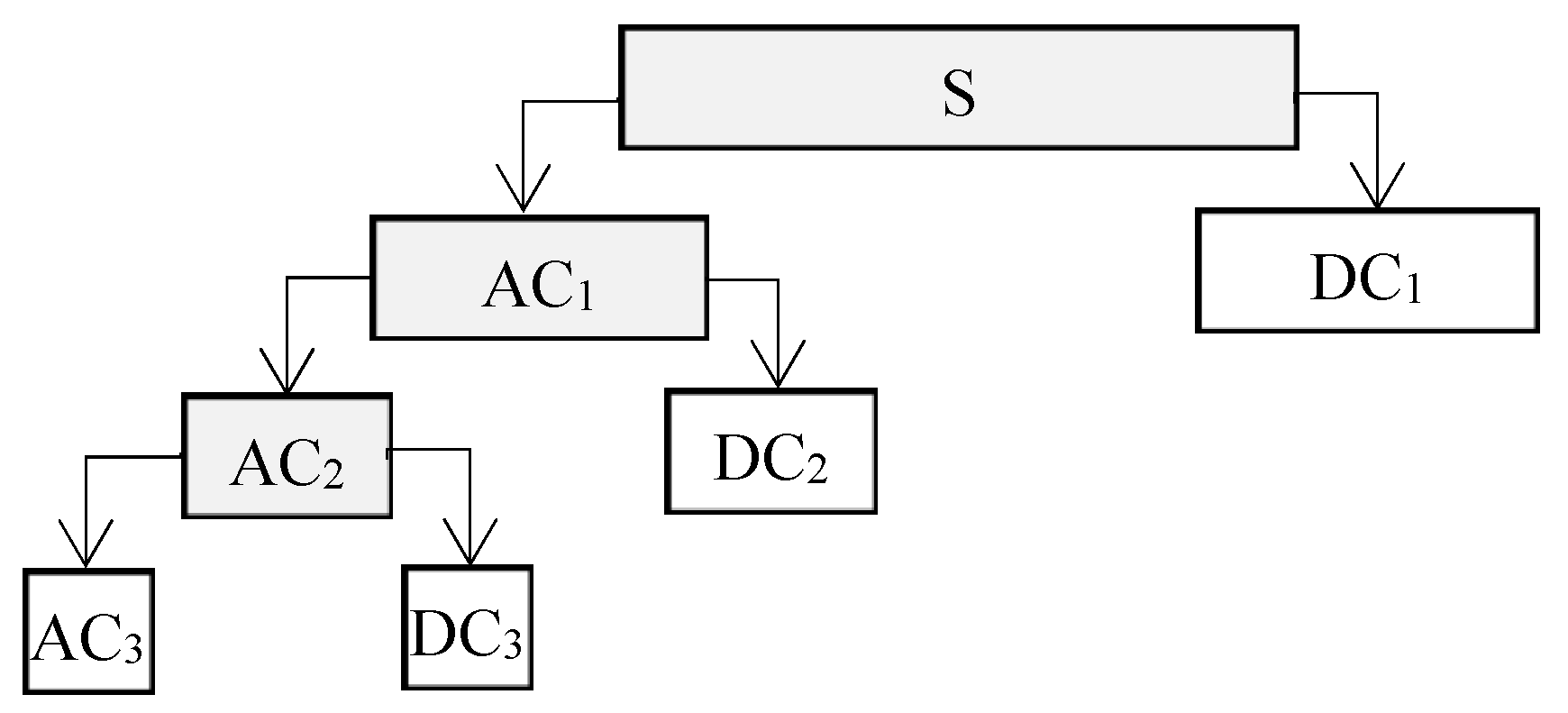
In practice, the wavelet basis performs as a set of high-pass and low-pass filters to decompose the signal into low-scale, high-frequency detail coefficients (DCs) and high-scale, low-frequency approximation coefficients (ACs) according to scale. The length of the ACs and DCs is related to the type of mother wavelet and decomposition level. In a multi-level decomposition, the filtering process can be iterated with successive approximations being decomposed in turn, so that the signal is broken down into many lower resolution components (Figure 1). Through the DWT, not only can the detailed behavior be separated from the macroscopic behavior, but also the dimensionality of hyperspectral data is reduced. All the information in the original signal is contained in the ACs at a particular decomposition level i (L_i) plus the DCs at decomposition level 1 to level j (L₁–L_i).

Considering the canopy spectrum as a signal changing with wavelength, the ACs and DCs after multi-level DWT decomposition were investigated as feature parameters of canopy spectra to find whether it is a productive tool for LNC estimation in this paper. DWT analysis could be implemented with the function ‘wavedec’ in MATLAB Wavelet Toolbox. The function, ‘wrcoef’, was used to reconstruct the spectral signal so as to find out how ACs delineate the canopy spectral information. Energy value (EV) [30] is a set of compressed ACs and DCs, which tries to take advantage of ACs and DCs to characterize the whole signal information. It also can be considered as a feature parameter of canopy hyper-spectral signal and can be obtained through the expression (3):

$$E{V}_i=\sqrt{\frac{1}{K}{\displaystyle \sum _{k=1}^K{w_{i,k}}^2}},$$

(3)

where EV_i denotes the wavelet energy value of the ith decomposition level (L_i), w_i,k is the kth wavelet coefficient at L_i and K represents the total number of wavelet coefficients under each level. As shown in Figure 1, EV₃ will be calculated with the AC₃, DC₁, DC₂ and DC₃ according to expression (3). Five mother wavelet functions including db10, sym8, coif5, bior6.8 and rbio6.8 from the Daubechies, Symlet, Coiflet, Biorthogonal and Reverse biorthogonal wavelet families, respectively, were assessed in this study, which are commonly tested wavelet families in the canopy spectra decomposition [25,26,27,28,30].

2.3.2. Existing Spectral Indices Calculation

A total of ten correlated hyperspectral indices from three categories were selected and examined for comparison with the DWT approach, including (1) chlorophyll indices: Modified red edge simple ratio index (mSR₇₀₅), MERIS terrestrial chlorophyll index (MTCI), structurally insensitive pigment index (SIPI) and normalized pigment chlorophyll index (NPCI); (2) nitrogen indices: Nitrogen reflectance index (NRI), normalized difference red-edge index (NDRE) and double-peak canopy nitrogen index (DCNI); (3) greenness indices: Green normalized difference vegetation index (GNDVI), optimized soil-adjusted vegetation index (OSAVI) and modified triangular vegetation index (MTVI₂). The definitions and reference sources for these ten spectral indices are summarized in

Table 1. The definitions and reference sources of narrowband spectral indices tested in this study.

Category	Index	Formula	Developed by
Chlorophyll indices	mSR705	(R750 – R445)/(R705 − R445)	[19]
	MTCI	(R754 − R709)/(R709 − R681)	[35]
	SIPI	(R800 − R445)/(R800 − R680)	[36]
	NPCI	(R430 − R680)/(R430 + R680)	[36]
Nitrogen indices	NRI	(R570 − R670)/(R570 + R670)	[37]
	NDRE	(R790 − R720)/(R790 + R720)	[38]
	DCNI	(R720 − R700)/(R700 − R670)/(R720 − R670 + 0.03)	[20]
Greenness indices	GNDVI	(R750 − R550)/( R750 + R550)	[39]
	OSAVI	1.16(R800−R670)/(R800 + R670 + 0.16)	[40]
	MTVI2	1.5(1.2(R800 − R550) − 2.5(R670 − R550))/sqrt((2R800 + 1)2 − (6R800 − 5sqrt(R670)) − 0.5)	[41]
Ri is the reflectance at i nm wavelength

.

2.3.3. Modeling Method

The ordinary least squares (OLS) regression analysis was used to construct the LNC estimation model based on sensitive-band reflectance and spectral index. Two types of multivariate models, partial least squares (PLS) regression and random forest (RF) regression, were carried out to establish the estimation model on the basis of wavelet coefficients and energy values.

PLS regression is a bilinear multivariate regression method. It compresses the input data into a number of independent latent variables (LVs) and maximizes the covariance between the LV scores and dependent variables. The operation makes it possible to avoid high collinearity among multi-variables and shows better prediction performance when compared with stepwise regression or principal component regression [21,42]. The basic PLS algorithm could be obtained in Geladi and Kowalski [43]. The number of latent variables is selected on the basis of the standard error of leave-one-out cross-validation. Parameter optimization and modeling were implemented with the PLS Toolbox based on MATLAB^® 7.0 (MathWorks, Inc., Natick, MA, USA).

RF regression is an ensemble machine learning algorithm based on regression trees [44,45]. It uses the bootstrap sampling method and randomized subspace method to build decision trees, in which only randomly selected predictors are used for each tree. The final prediction result is determined by the average of all decision trees. Two parameters need to be optimized in RF: ‘ntree’, the number of regression trees grown based on a bootstrap sample of the observations; ‘mtry’, the number of different predictors (independent variables) tested at each node. The random forest library developed in the R package (R Development Core Team 2008) was employed to implement the RF algorithm in this study. The parameter ‘mtry’ was set as 1/3 of the number of independent variables and the ‘ntree’ was set at 500 as suggested by Breiman [43].

2.3.4. Calibration and Validation

In order to ensure the range of LNC is represented in both datasets, all the observations were pooled together and then divided into calibration and validation dataset according to LNC values in an ascending sort order with a proportion of 4:1 [46]. The calibration and validation data sets were evenly distributed (

Table 2. The statistical description of leaf nitrogen concentration (%) across all growth stages.

Data Set	No. of Samples	Min	Max	Range	Mean	SD	Variance	Skewness	Kurtosis	CV (%)
Whole	315	0.22	3.87	3.64	1.47	0.77	0.59	0.76	2.98	52.03
Calibration	252	0.22	3.60	3.38	1.46	0.76	0.58	0.73	2.88	51.88
Validation	63	0.35	3.87	3.52	1.5	0.79	0.63	0.86	3.26	53.00

). LNC ranged from 0.22% to 3.87% across all growth stages, with an average value of 1.47%. The coefficient of variation (CV) was 52.03% indicating a moderate temporal variation.

The coefficient of determination (R²), root mean square error (RMSE), relative error (RE, %) and the ratio of prediction to deviation (RPD) were used to measure the predictive performance of each estimation model by different methods. Higher values of R² and RPD, and lower values of RMSE and RE indicate better dependability and accuracy of the regression model in predicting LNC [21,47,48]. RPD is a ratio of standard deviation to RMSE. RPD values greater than 2.0 indicate a stable and accurate predictive model, an RPD value between 1.4 and 2.0 indicates a fair model that could be improved by more accurate prediction techniques and a value less than 1.4 indicates poor predictive capacity [21]. Rc², Rv², RMSEc, RMSEv, REc, REv, RPD_c and RPD_v in this paper represented R², RMSE, RE and RPD in the calibration and validation data set, respectively. A 1:1 plot of observed vs. estimated values was drawn to demonstrate the degree of model fit.

3. Results

3.1. LNC Estimation Models (SR-LNC) Based on Sensitive-Band Reflectance

3.1.1. Correlations Between Canopy Spectra and LNC

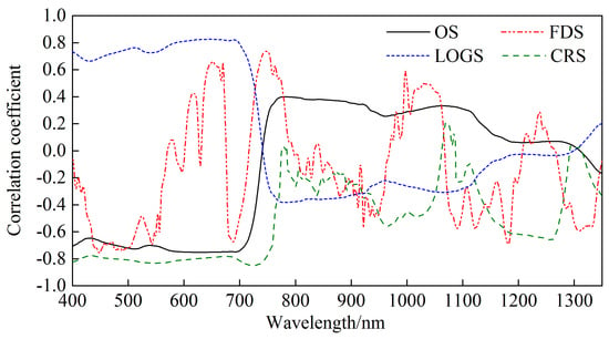
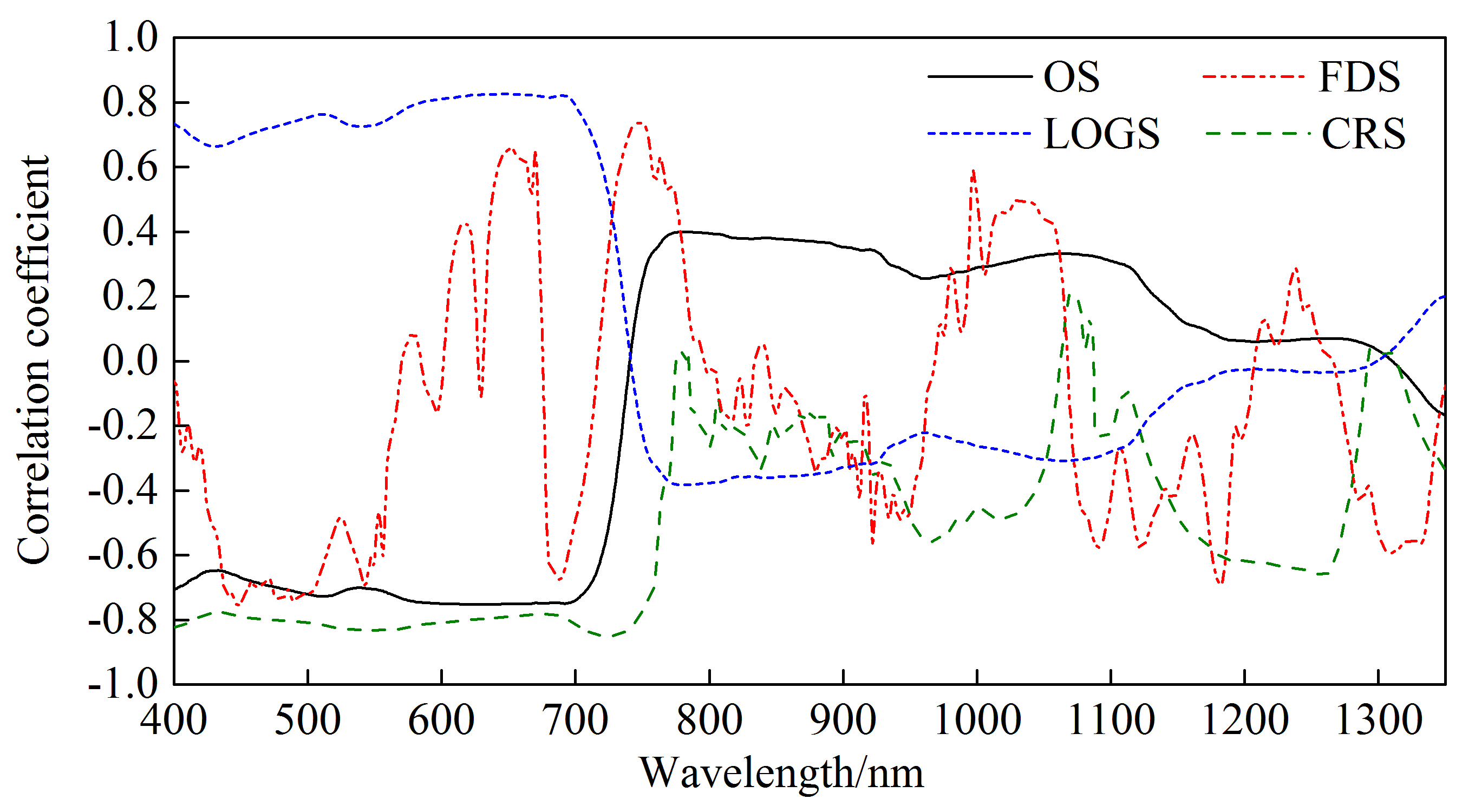
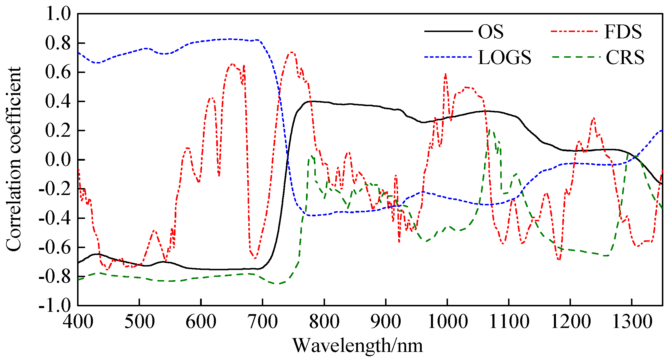
In general, winter wheat canopy reflectance was more significantly correlated with LNC at VIS than NIR wavelengths (Figure 2). The absolute values of the correlation coefficient were greater than 0.6 at 400–750 nm. Correlations were similar from 614 to 640 nm, with the strongest negative value of −0.75. The correlation between FDS and LNC changed rapidly at 400–1300 nm. It was slightly better at 435–465 nm than other wavelengths, and the best correlation coefficient was −0.76 at 447 nm. A weak negative correlation between LOGS and LNC was found in the near-infrared region (750–1300 nm), whereas a strong positive correlation was observed at 400–750 nm, which significantly improved the relationship between OS and LNC at 600–700 nm. The highest correlations appeared at 642–648 nm with a correlation coefficient of 0.83. Correlation between CRS and LNC was better at 400–765 nm, 934–1050 nm, 1124–1290 nm and 1304–1350 nm than that between OS and LNC. Moreover, the correlation coefficients were greater than 0.6 at 400–760 nm and 1180–1270 nm, and the best correlation coefficient was −0.85 at 721–727 nm. As reflectance at 640 nm was affected by chlorophyll absorption [8], and 725 nm within the red-edge wavelength region was highly related with canopy nitrogen content [17], 640 nm and 725 nm were selected as the bands of OS and CRS most sensitive to LNC, respectively. According to the best correlation with canopy spectra, 447 nm and 645 nm (center part of 642–648 nm) were regarded as the bands of FDS and LOGS most sensitive to LNC, respectively. The spectral reflectance of sensitive bands is used to establish LNC estimation models.

3.1.2. Construction of SR-LNC Estimation Models

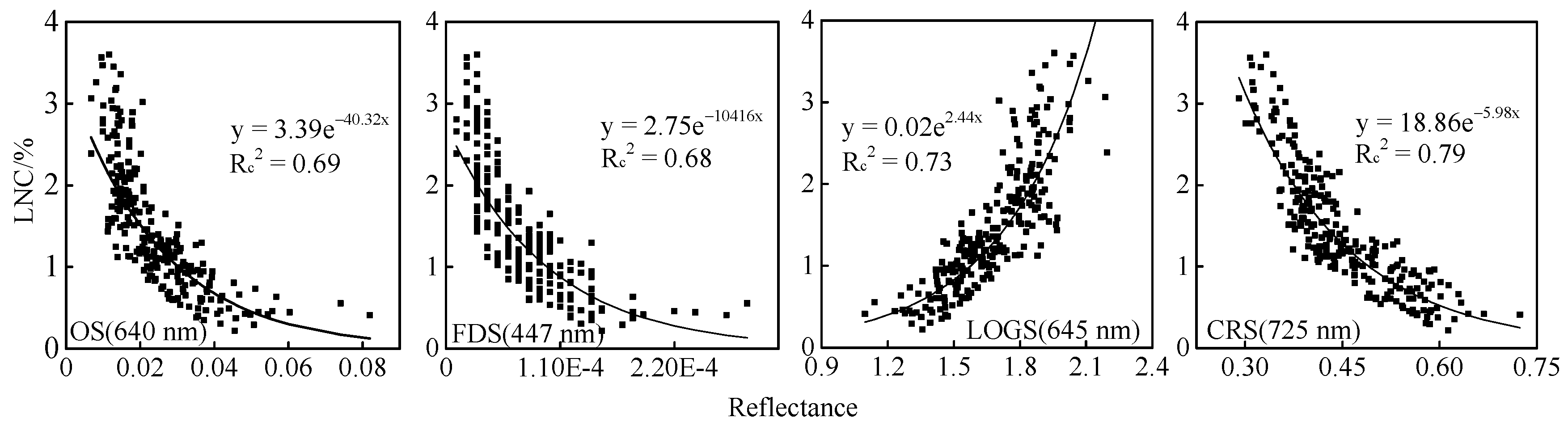
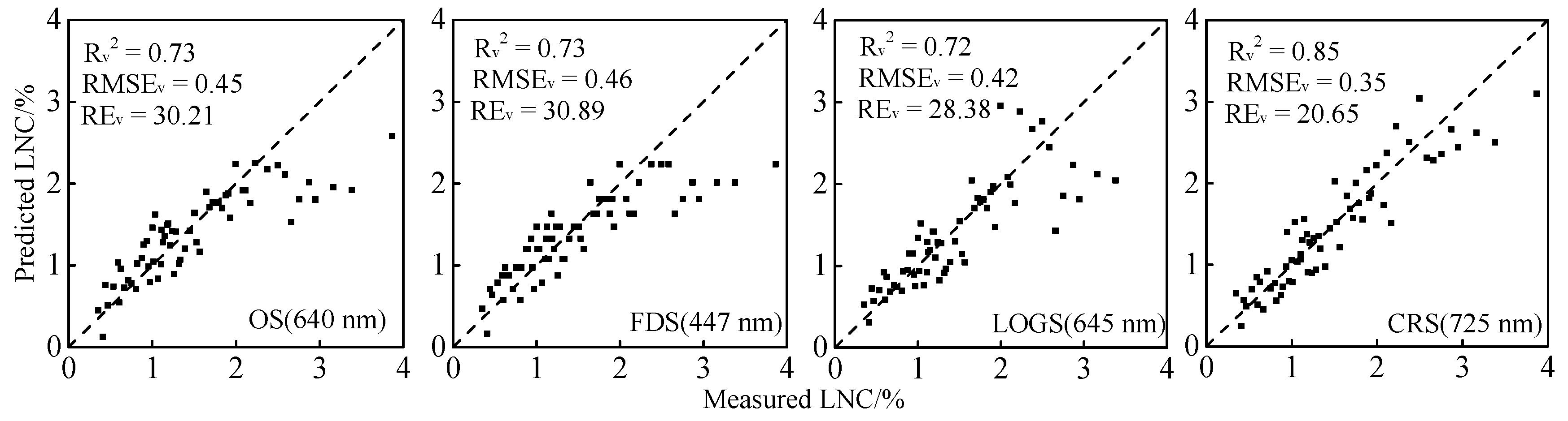
The calibration and validation accuracy of FDS at 447 nm and OS at 640 nm were similar to each other (Figure 3; Figure 4). LOGS at 645 nm and CRS at 725 nm significantly improved the LNC prediction accuracy relative to the FDS and OS models, and the R_c²s in exponential prediction models were 0.73 and 0.79, respectively. The R_v²s in validation samples were 0.72 and 0.85, RMSE_vs were 0.42 and 0.35 and RE_vs were 28.38 and 20.65 for LOGS and CRS, respectively. Scatter plots between predicted and measured LNC values indicated that higher LNC values were underestimated (Figure 4). CRS was superior to other spectra in predicting LNC at sensitive reflectance bands, with predicted and measured LNC values falling close to the 1:1 line.

3.2. LNC Estimation Models (SI-LNC) Based on Spectral Indices

All the spectral indices were significantly correlated with LNC as shown in

Table 3. Estimation models and prediction errors of leaf nitrogen concentration based on the spectral indices. ** at 0.01 significance level.

Category	Index	Correlation Coefficient	Equation	Rc2	Rv2	RMSEv	REv
Chlorophyll indices	mSR705	0.91 **	LNC = 0.2702x − 0.6773	0.83	0.86	0.28	18.81
	MTCI	0.89 **	LNC = 0.5454x − 1.0901	0.78	0.84	0.31	20.94
	SIPI	0.79 **	LNC = 1E − 06e15.28x	0.71	0.69	0.57	37.80
	NPCI	0.80 **	LNC = 1.9583e4.13x	0.70	0.71	0.45	30.13
Nitrogen indices	NRI	0.70 **	LNC = 6.2342x − 0.5199	0.50	0.50	0.56	37.64
	NDRE	0.86 **	LNC = 0.046e6.28x	0.80	0.85	0.30	20.27
	DCNI	0.79 **	LNC = 0.039x − 0.8904	0.63	0.74	0.41	27.06
Greenness indices	GNDVI	0.85 **	LNC = 0.002e8.44x	0.81	0.82	0.33	21.90
	OSAVI	0.69 **	LNC = 0.0099e6.61x	0.55	0.54	0.55	36.61
	MTVI2	0.60 **	LNC = 5.293x − 1.0551	0.36	0.42	0.60	40.08

. The mSR₇₀₅ index was the best of ten spectral indices, which could explain 83% variability in LNC. The higher R_v² (0.86), lower RMSE_v (0.28) and RE_v (18.81) also illustrated a better performance of mSR₇₀₅. The NDRE index was the best of three nitrogen indices, which could explain 80% of variability in LNC. The GNDVI was the best among the three greenness indices. Both GNDVI and NDRE were exponentially related to LNC, while the accuracy of GNDVI was slightly worse than NDRE.

3.3. LNC Estimation Models (DWT-LNC) Based on DWT Features

3.3.1. Selection of Optimum Mother Wavelet and Decomposition Level

The number of DWT coefficients describes the extent of data compression. As shown in

Table 4. The number of wavelet coefficients under different mother wavelets and decomposition levels.

Mother Wavelet	L1	L2	L3	L4	L5	L6	L7	L8	L9	L10	L11	L12
bior6.8	484	250	133	75	46	31	24	20	18	17	17	17
coif5	490	259	144	86	57	43	36	32	30	29	29	29
db10	485	252	135	77	48	33	26	22	20	19	19	19
rbio6.8	484	250	133	75	46	31	24	20	18	17	17	17
sym8	483	249	132	73	44	29	22	18	16	15	15	15

, the number of DWT coefficients changed with the mother wavelet and decomposition level, and was independent on spectral transformation types. It tended to drop off from L₁ to L₁₂, and the downward trend became stable at L₁₀. Among five mother wavelets, sym8 had the strongest data compression ability, while coif5 was the weakest. For example, the total number of wavebands in this study was 951 (from 400–1350 nm). After DWT analysis at decomposition level 10, the number of DWT coefficients with mother wavelet function sym8 was 15, while coif5 had 29, which was determined from the wavelet basis length [25].

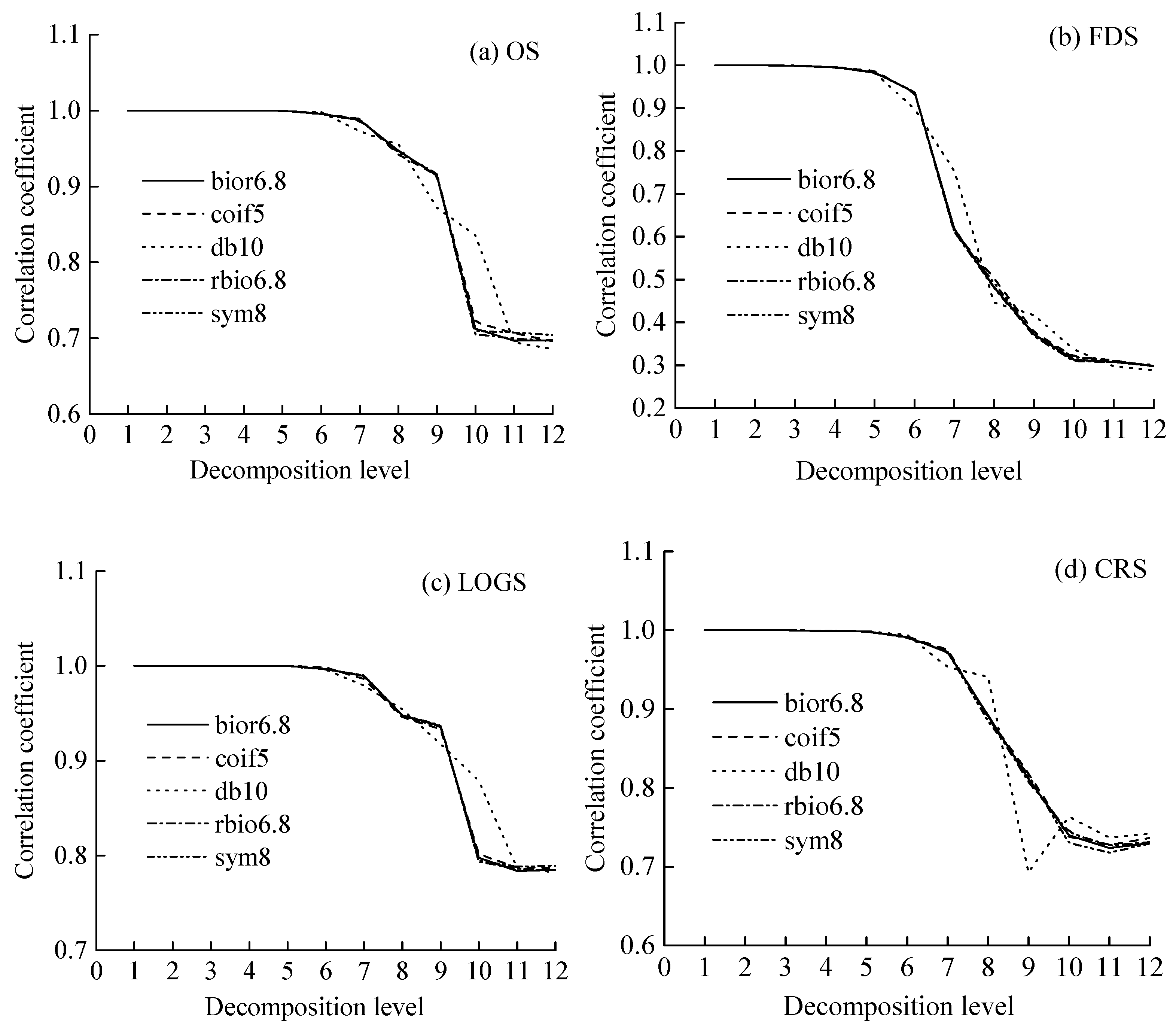
Since the approximation coefficient (AC) was considered as an indicator of global information for the canopy spectrum, ACs of each transformed spectrum at decomposition level 1 to 12 were utilized to perform signal reconstruction in order to find out how ACs delineated the canopy reflectance spectra. The correlations between canopy spectral signals and reconstruction signals are shown in Figure 5. The correlation coefficient decreased from L₅ until leveling off at L₁₀, which indicated that the explanatory and signal restoring ability of ACs to canopy spectra declined gradually from L₅ to L₁₀. All the correlation coefficients were still above 0.7 at L₁₀ except with FDS, which went down to less than 0.6 rapidly after decomposition level 6. The mother wavelet db10 was more labile compared to the others, especially poor was the large fluctuation in CRS correlations. Taking into account the data compression effectiveness, stability of mother wavelet and ability to maintain the information quality of the canopy spectra, a mother wavelet sym8 at decomposition level of L₁–L₁₀ was chosen to conduct the DWT to analyze the correlation with LNC.

3.3.2. DWT-LNC Models Based on PLS Regression

PLS Regression Using Wavelet ACs

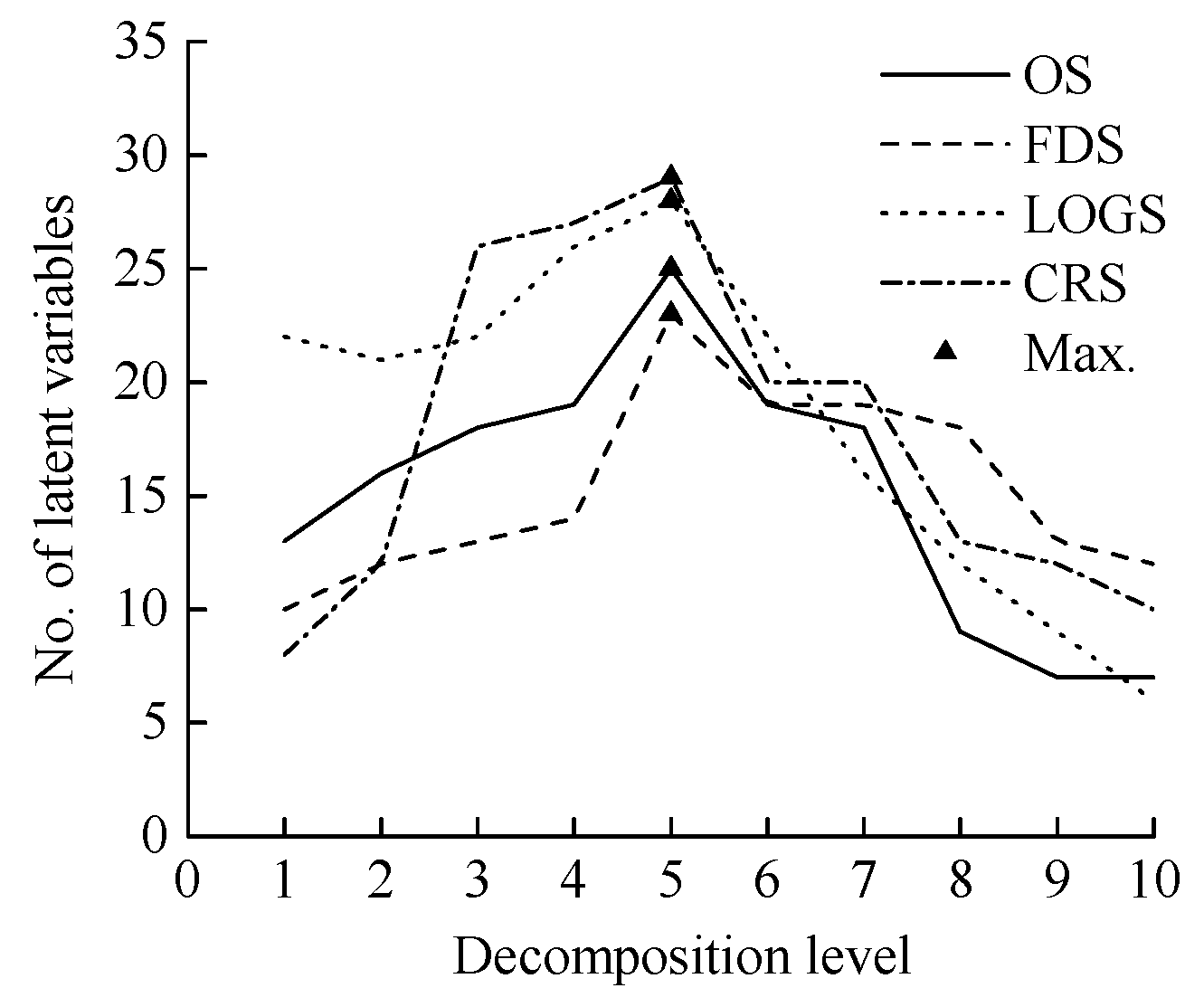
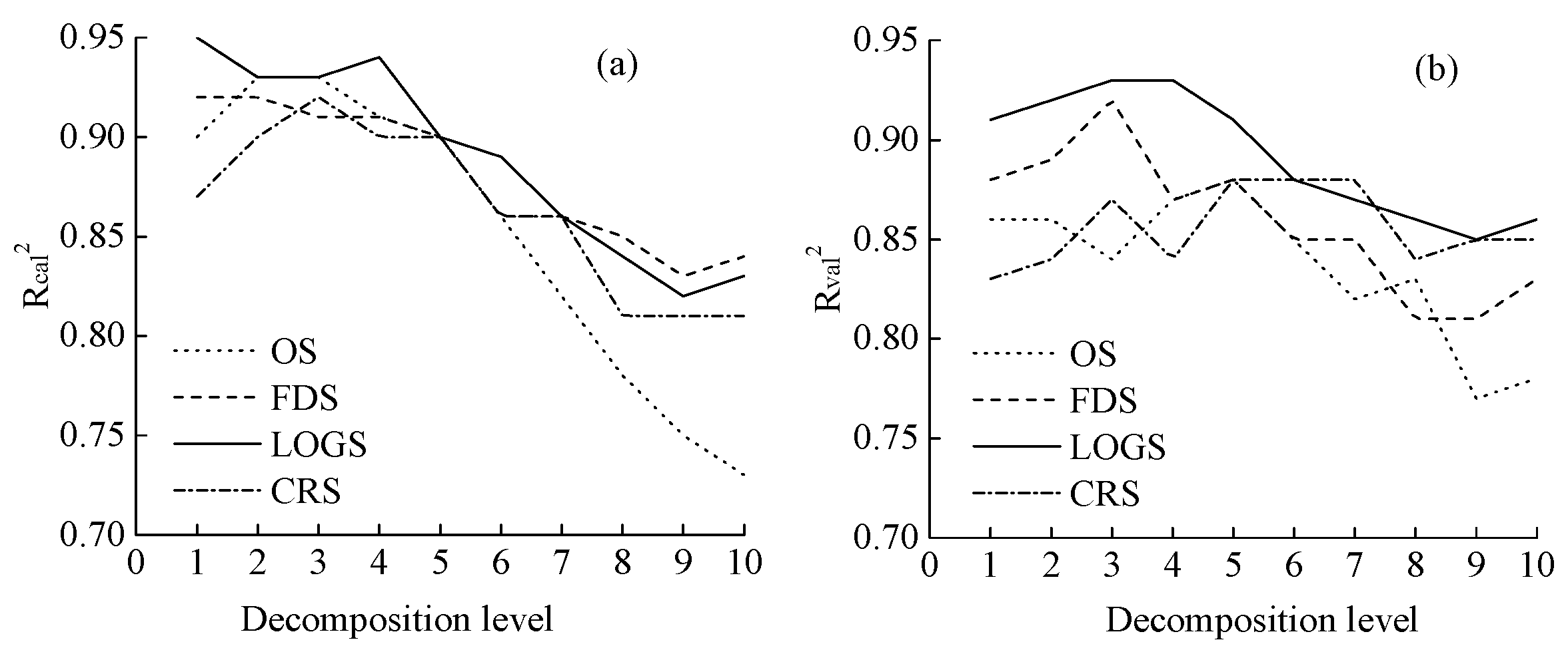
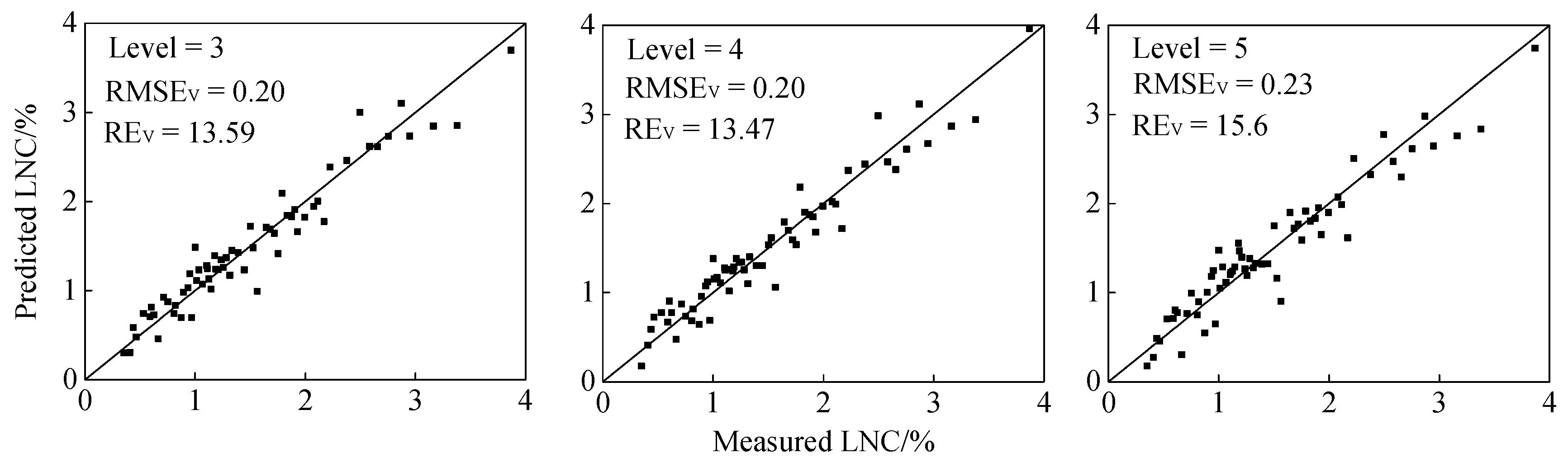
All the LNC estimation models established by calibration of sample measurements with ACs of sym8 at L₁ to L₁₀ passed the 0.01 significance level test. The number of latent variables (LVs) extracted by PLS regression increased and then decreased with the decomposition level (Figure 6). The maximum number of latent variables emerged at L₅, which implied a lower convergence rate of the PLS regression at L₅. As a whole, all the estimating models had high prediction accuracy (R_c² was greater than 0.70). The general trend of R_c² in each predicting model increased and then decreased gradually with an increasing decomposition level (Figure 7). The ACs could explain 90%–93% of the variability in LNC at L₁ to L₅, except with CRS at L₁. The variation of R_v² was consistent with R_c², and all the R_v²s were greater than 0.75.

Table 5. The coefficient of determination, root mean square error and relative error of the validation set based on a partial least squares regression with wavelet approximation coefficients.

	OS			FDS			LOGS			CRS
	Rv2	RMSEv	REv	Rv2	RMSEv	REv	Rv2	RMSEv	REv	Rv2	RMSEv	REv
AC1	0.86	0.29	19.59	0.88	0.27	18.07	0.91	0.24	15.78	0.83	0.33	22.06
AC2	0.86	0.30	19.68	0.89	0.26	17.22	0.92	0.23	15.19	0.84	0.33	22.13
AC3	0.84	0.32	21.24	0.92	0.23	15.50	0.93	0.20	13.59	0.87	0.33	22.18
AC4	0.87	0.29	19.09	0.87	0.27	18.18	0.93	0.20	13.47	0.84	0.33	22.20
AC5	0.88	0.28	18.45	0.88	0.29	19.49	0.91	0.23	15.60	0.88	0.28	18.37
AC6	0.85	0.31	20.98	0.85	0.31	20.76	0.88	0.27	17.95	0.88	0.27	18.24
AC7	0.82	0.34	22.62	0.85	0.31	20.52	0.87	0.30	20.11	0.88	0.27	17.99
AC8	0.83	0.33	22.28	0.81	0.31	20.84	0.86	0.30	19.83	0.84	0.31	20.87
AC9	0.77	0.38	25.13	0.81	0.35	23.07	0.85	0.30	20.29	0.85	0.31	20.74
AC10	0.78	0.37	24.90	0.83	0.32	21.64	0.86	0.29	19.59	0.85	0.30	20.14

shows the variation in RMSE and RE. LOGS had stronger prediction ability over other models, with the highest values of R_v² and R_c², and lowest RE_v and RMSE_v values at L₁–L₁₀. All the RMSE_vs were below 0.30. The R_v²s were 0.93, 0.93 and 0.91 respectively for the LOGS at L₃, L₄ and L_5. Measured and predicted LNC values with ACs from LOGS at L₃–L₅ closely approximated a 1:1 line (Figure 8), and the PLS model at L₄ yielded the optimal prediction accuracy (RMSE_v = 0.20, RE_v = 13.47).

PLS Regression Using Wavelet DCs

The high-frequency detail coefficient of DWT analysis represented noise or minor absorption in the canopy spectrum [21,28,49]. Figure 5 shows that the correlation coefficients between canopy spectral signals and reconstruction signals by ACs at decomposition level 1 to 5 were close to 1, which indicates that DCs at L₁ to L₅ were very small in amplitude (near zero) and could be removed without major loss in the information content of the signal.

Table 6. The coefficient of determination, root mean square error and relative error of the validation set based on a partial least squares regression with detail coefficients at decomposition level 6 to level 10. DC_i denotes the detail coefficient (DC) at L_i.

DC	OS			FDS			LOGS			CRS
	Rv2	RMSEv	REv	Rv2	RMSEv	REv	Rv2	RMSEv	REv	Rv2	RMSEv	REv
DC6	0.84	0.32	21.43	0.81	0.35	23.02	0.89	0.26	17.53	0.85	0.30	20.25
DC7	0.83	0.33	21.75	0.77	0.38	25.19	0.89	0.27	17.73	0.84	0.32	21.41
DC8	0.83	0.33	22.17	0.57	0.52	34.54	0.87	0.29	18.38	0.81	0.35	23.13
DC9	0.77	0.38	25.36	0.48	0.57	38.05	0.88	0.28	18.77	0.81	0.36	23.76
DC10	0.76	0.39	26.17	0.39	0.62	41.63	0.88	0.28	19.55	0.77	0.38	25.53

summarizes the validation results of PLS models based on DCs at L₆–L₁₀. Prediction accuracy decreased with the decomposition level. The performance of LOGS was better than other spectral transformations, but it was still worse than PLS modeling with ACs (Table 5).

PLS Regression Using EVs

Energy values achieve further compression of spectral signals. After multi-level one-dimensional wavelet analysis at decomposition level n, n + 1 variables were used to calculate the energy value according to Equation (3), and the relationship between energy value and LNC was analyzed by using PLS regression (

Table 7. The coefficient of determination, root mean square error and relative error of the validation set based on a partial least squares regression with wavelet energy values. EV_i denotes energy value (EV) at decomposition level i.

EV	OS			FDS			LOGS			CRS
	Rv2	RMSEv	REv	Rv2	RMSEv	REv	Rv2	RMSEv	REv	Rv2	RMSEv	REv
EV1	0.14	0.73	49.02	0.46	0.58	38.83	0.47	0.57	38.22	0.64	0.47	31.61
EV2	0.25	0.69	46.14	0.43	0.59	39.80	0.72	0.42	28.67	0.71	0.43	28.43
EV3	0.19	0.71	47.34	0.41	0.61	40.58	0.71	0.44	29.36	0.72	0.41	27.66
EV4	0.19	0.71	47.34	0.36	0.63	42.08	0.65	0.46	31.14	0.74	0.40	26.74
EV5	0.29	0.67	44.42	0.32	0.65	43.47	0.69	0.43	29.05	0.75	0.39	26.34
EV6	0.74	0.42	27.93	0.65	0.47	26.41	0.81	0.34	22.85	0.75	0.39	26.41
EV7	0.79	0.36	23.99	0.66	0.47	31.49	0.81	0.34	22.91	0.76	0.38	25.88
EV8	0.87	0.29	19.22	0.74	0.41	27.61	0.83	0.32	21.56	0.80	0.35	23.56
EV9	0.87	0.29	19.15	0.76	0.40	27.02	0.84	0.32	21.35	0.81	0.34	23.19
EV10	0.87	0.29	19.28	0.82	0.35	23.23	0.88	0.26	17.82	0.83	0.33	22.17

). With an increase in decomposition level, R_v² increased and then decreased with OS and LOGS, while a general tendency of first increasing then decreasing and a conspicuous monotonic increase were found, respectively, with FDS and CRS (Table 7). However, all the R_v² reached the maximum at L₁₀. Energy value could explain over 80% of the variability of LNC at L₁₀ with fewer variables (number of variables was 11). LOGS still gave the best performance over the other transformations (with R_c² of 0.85 and R_v² of 0.88), but the overall accuracy was still lower than those using approximate coefficients at L₃–L₅ (Figure 6). The RMSE and RE of validation set were 0.26 and 17.82 respectively, also a poorer correlation compared with the results in Table 5.

3.3.3. DWT-LNC Based on RF Regression

ACs and EV₁₀ were selected to build the RF regression models. As showed in

Table 8. Validation of leaf nitrogen concentration estimation models based on a random forest regression with discrete wavelet transform features. AC_i denotes approximation coefficient (AC) at Li; EV₁₀ is the energy value at L₁₀.

	OS			FDS			LOGS			CRS
	Rv2	RMSEv	REv	Rv2	RMSEv	REv	Rv2	RMSEv	REv	Rv2	RMSEv	REv
AC1	0.86	0.29	19.64	0.87	0.29	19.30	0.89	0.26	17.53	0.89	0.27	17.93
AC2	0.86	0.30	19.86	0.87	0.29	19.25	0.89	0.27	17.91	0.89	0.28	18.38
AC3	0.87	0.29	19.34	0.87	0.29	19.20	0.89	0.26	17.21	0.88	0.28	18.41
AC4	0.86	0.29	19.52	0.86	0.29	19.52	0.91	0.24	16.08	0.89	0.27	17.78
AC5	0.87	0.28	18.89	0.87	0.29	19.01	0.90	0.25	16.35	0.89	0.28	18.44
AC6	0.86	0.28	18.91	0.86	0.29	19.44	0.86	0.28	18.40	0.88	0.29	19.25
AC7	0.88	0.29	19.41	0.71	0.43	28.76	0.86	0.30	20.12	0.86	0.31	20.77
AC8	0.83	0.33	21.84	0.69	0.45	29.85	0.85	0.31	20.84	0.84	0.32	21.57
AC9	0.85	0.31	20.67	0.64	0.49	32.45	0.80	0.36	24.02	0.81	0.35	23.27
AC10	0.83	0.32	21.49	0.51	0.56	37.15	0.74	0.41	27.17	0.76	0.39	26.23
EV10	0.82	0.35	23.34	0.77	0.38	25.36	0.86	0.29	19.43	0.84	0.32	21.16

, R²s in the validation set were slightly lower than the calibration set and most of them were less than 0.90, except for results using ACs of LOGS in L₄ and L₅. After L₅, the RMSE_v and RE_v tended to go up slightly for all transformations especially with FDS. In general, LOGS was better than other transformations in estimating LNC by ACs with RF regression. ACs at L₄ had the best RMSE_v and RE_v, being 0.24 and 16.08, respectively, while the ACs at L₁₀ were the worst in the RF regression models. The accuracy of RF models based on energy values of wavelet coefficients was improved compared with the PLS regression, but still poorer than using ACs.

3.4. Estimation Accuracy Comparison

Compared with OS at 640 nm, the sensitive band reflectance of CRS at 725 nm provided a significant improvement in the accuracy of estimating LNC. The R_c² and R_v² increased to 0.79 and 0.85, and the RMSE_v and RE_v decreased to 0.35 and 20.65, respectively (Figure 2). The accuracy also was better than the results of LOGS and FDS at 645 nm and 447 nm, respectively (Figure 3 and Figure 4). However, it was still lower than the performance of some spectral indices especially mSR₇₀₅ (R_c² = 0.83, R_v² = 0.86, RMSE_v = 0.28 and RE_v = 18.81; Table 3). The LOGS was obviously distinguished from four transformed canopy spectra in the discrete wavelet transform analysis and exhibited a promising potential for revising LNC. For PLS modeling, LOGS combined with ACs at L₄ produced the best performance both in the calibration and validation sets. The prediction result of LNC in the high-value region was better than SR-based and SI-based LNC estimation models. DCs and EVs performed worse in LNC evaluation by using PLS regression. The best prediction accuracy of DCs was at the decomposition level 6 (R_v² = 0.89, RMSE_v = 0.26 and RE_v = 17.53), which was slightly higher than the mSR₇₀₅ index. EVs at L₁₀ had similar prediction accuracy as DCs at L₆. With RF regression, LOGS at L₄ showed the highest accuracy in LNC prediction on the basis of ACs, with the R_v², RMSE_v and RE_v being 0.91, 0.24 and 16.28, respectively, which were slightly worse than the PLS regression. LNC estimation result using energy values was improved by a RF regression, but it was still lower than the PLS and RF models with ACs at L₄.

The ration of prediction to deviation (RPD) is calculated by dividing the standard deviation (SD) of the reference data by the standard error of prediction. Since the SD values for calibration and validation data set are constants, the RPD value will not change the ranking of best performing indicators. However, the RPD is a dimensionless parameter and can be classified to different categories to evaluate the model accuracy.

Table 9. The ratio of prediction to deviation (RPD) values in the calibration models and validation models of leaf nitrogen concentration.

Model	OLS regression		PLS regression			RF regression
	CRS725	mSR705	AC4	DC6	EV10	AC4	EV10
RPDc	1.95	2.43	3.97	2.81	2.61	3.04	2.38
RPDv	2.26	2.82	3.95	3.04	3.04	3.29	2.72

exhibited the RPD values in some of the estimation models. All the RPDs in the calibration set and validation set exceeded 2.0 except the OLS regression model based on the CRS₇₂₅, which indicated all the estimation models in Table 9 had stable and accurate predictive abilities. The PLS model with AC₄ produced the best performance (RPD_c = 3.97 and RPD_v = 3.95), and followed by the RF regression model with AC₄ (RPD_c = 3.04 and RPD_v = 3.29). Overall, by comparing all the methods in this article with statistical indicators of R², RMSE, RE and RPD, an integrated approach using DWT ACs and PLS regression exhibited the highest stability and reliability in LNC estimation.

4. Discussion

A large number of studies have been conducted with passive and active remote sensing technologies for the timely and non-destructive evaluation of LNC [9,10,11,13,14,15,16,17,50]. In the present study, we mainly discussed the effect of the entire range of canopy reflectance (400–1350 nm) on LNC estimation and provided a guide for feature extraction by DWT analysis and PLS regression.

4.1. Sensitive Band Reflectance and Spectral Transformation

This study demonstrated that spectral measurements were apparently useful for describing the N status of wheat canopies. It is known that pure chlorophyll a and b had absorption peaks at red and blue wavelength regions, respectively. The red edge (680–760 nm) caused by the strong absorption of pigments in the red spectrum and leaf scattering in the NIR spectrum has been found to be sensitive to crop growth [12,14,16,17,18]. As N concentration was linked to the plant photosynthetic pigments concentration especially chlorophyll, the correlation between leaf nitrogen concentration and spectral reflectance in visible light was better than in the near-infrared region as shown in Figure 2. All the sensitive wavebands of spectral transformations were located in visible light (OS at 640 nm, FDS at 447 nm, LOGS at 645 nm and CRS at 725 nm). In previous research, the first derivative was closely related to N concentration in corn and wheat [20], which was designed to eliminate background signals or noise and to resolve overlapping spectral features. The LOG transformation performed accurately compared with the original reflectance when estimating N concentrations [14]. CRS yielded the highest accuracy in estimating grass leaf nitrogen concentrations, followed by the LOGS [51]. Continuum removal enhanced the differences in absorption strength [34]. All indicated that spectral transformation could provide more sensitive features than canopy original spectrum and could be used to increase the accuracy of crop N estimation. We compared the LNC estimation accuracy of these four spectral transformations in this study. The result showed the performance of CRS (R_c² = 0.79) was higher than that of LOGS, FDS and OS (Figure 3) in winter wheat LNC prediction. The same conclusion was obtained in the grass foliar nitrogen retrieval reported by Ramoelo et al. [51], where an R² of 0.81 was based on a greenhouse experiment using continuum removal in combination with a PLS regression. As a whole, the exponential model was more suitable for delineating the quantitative relationship between sensitive band reflectance and LNC than a linear regression (Figure 3). This may be caused by the fact that the relationship between leaf N and chlorophyll concentration was not linear [10,52].

4.2. Relationship Between Spectral Indices and LNC

Canopy spectra obtained by remote sensing were affected by the canopy structure and surrounding conditions, while the spectral index could eliminate the impacts at a certain extent through the combination of characteristic bands [12]. Reflectance in the red-edge region (680–760 nm) was closely related to the chlorophyll content in plants as well as the nutritional status of plants, which had always been considered to be important in relationships with biochemical or biophysical parameters [53]. The mSR₇₀₅ index of chlorophyll indices, NDRE index of nitrogen indices and GNDVI of greenness indices in this paper were constructed on the basis of red edge reflectance, could explain 83%, 80% and 81% of the variability in LNC, respectively (Table 3), and had better performance than other spectral indices. This was consistent with the report that the GNDVI performed similarly as NDRE in estimating maize N concentration [52]. Green and red edge reflectance were sensitive to a wider range of chlorophyll levels than red reflectance. The predictive ability of NDRE in the category of nitrogen indices was higher than with NRI and DCNI in this study (Table 3). NDRE is similar in form to NDVI, but with the red band being replaced by a red edge band. NRI, a normalized near-infrared over green waveband reflectance ratio, has been used to assess in-season corn N status and to develop N variability maps [37,54], but in our study, the predictive ability (R_c² = 0.50) of NRI was lower than NDRE (R_c² = 0.80). These results demonstrated the importance of red edge vegetation indices for estimating winter wheat N status.

Three-band spectral indices were proposed to solve the saturation problem associated with two-band indices [18,55,56]. Chen et al. [20] developed the three-band spectral index DCNI using the double-peak characteristics of the red edge to predict the nitrogen content of maize and wheat showed the determination coefficient of the prediction equation being 0.72 and 0.44, respectively. However, the DCNI (R_c² = 0.63) explained 20% less variability in LNC than mSR₇₀₅ in this study (Table 3). The RMSE of mSR₇₀₅ (RMSE_v = 0.28) indicated an ordinary performance of the LNC prediction model, and an RMSE_v of 0.41 indicated poor model performance of DCNI [48].

4.3. Features and Parameters Selection of the DWT Analysis

The mother wavelet function and decomposition level were two crucial parameters required for DWT analysis. The scaled and translated mother wavelet was used to fit the canopy spectra. Cocchi et al. [57] demonstrated the difficulty in developing a priori rules for identifying the most appropriate mother wavelet because the optimum mother wavelet changed with the particular task [58]. Five commonly used mother wavelets in vegetation spectra decomposition were tested in this study. Results showed that the mother wavelet sym8 was excellent in dimensionality reduction and signal reconstruction than other wavelets. Features based on the sym8 made a good LNC estimation accuracy (Table 5, Table 6 and Table 7), which indicated the shape of the wavelet sym8 could explicate the differences between the LNC.

Three DWT features (AC, DC and EV) were extracted to analyze the relationship with LNC. The wavelet low-frequency approximation coefficient (AC) was a reflection of global features in canopy spectra, while the high-frequency detail coefficient (DC) was a depiction of noise information, which together contained all of the information presented in the original spectrum. Energy value (EV) was a set of compressed ACs and DCs, which tried to take advantage of ACs and DCs to express the whole signal information. Blackburn and Ferwerda [59] used the approximation coefficients at level 8 along with detail coefficients from level 1 to 8 to estimate chlorophyll concentration. However, most of the characteristic information of canopy spectra was in the approximation coefficients at a lower decomposition scale. For their study, DCs were very small in amplitude and could be removed without major loss in the information content of the signal kept in ACs. After a certain decomposition level, more and more useful information would be eliminated, contributing to noisy signals and declining information content of canopy reflectance spectra [59]. In contrast, we found that ACs in decomposition level 1 to 5 preserved almost 100% of the information features for the canopy spectra (Figure 5). Our results also illustrated that LNC was much better correlated with the main information in ACs, not DCs (Table 5; Table 6), so the ACs in L₁ to L₅ could be used directly to predict the LNC, instead of using the whole reflectance spectra, while ignoring the high-frequency DCs.

Energy value achieved a further data compression of canopy spectral signals. Pu and Gong (2004) [28] indicated that the energy value features extracted by the WT method were the most effective way of mapping forest crown closure (CC) and leaf area index (LAI). The mapped accuracy for CC was 84.90% and for LAI was 75.39%. In this study, the EVs at AC₄ with PLS regression could explain 83% (R_c² = 0.83) of the variability in LNC. EVs had a poorer performance and ability to estimate LNC compared with the ACs. This might be due to excessive dimensionality reduction, resulting in a loss of some sensitive information in the canopy spectrum.

Our results showed that the wavelet coefficients were different depending upon whether they were derived from the reflectance spectra or transformed spectra. The differences indicated that transformed spectra were more sensitive to LNC than original reflectance spectra (Table 5, Table 6, Table 7 and Table 8). The LOG-transformation was more useful in extracting additional information that was more difficult to obtain from other transforms of reflectance spectra.

4.4. Estimation Models of LNC

The results of this study indicated that the combination of multi-spectral bands generally improved the accuracy of LNC estimation (Table 4). The hyper-spectral narrow-band index (mSR₇₀₅) explained 4% more variability in LNC estimation than the best performing single sensitive band CRS₇₂₅. The advantage of multi-variable regression was obvious (Table 9). Approximation coefficients at decomposition level 4 using LOG-transformed spectra had the best prediction accuracy in PLS-LNC models. The prediction accuracy of the RF-LNC model with LOGS at L₄ was similar to the PLS-LNC model, while the R², RMSE, RPD and RE of validation set were slightly worse than the PLS regression (Table 8 and Table 9). That is, the prediction and verification accuracy of the PLS model was more stable than that of the RF model. This is likely because the accuracy of the RF model was greatly influenced by the undefined input parameters, although it was efficient for large input variables and non-linear problems [42,43,44,45].

All the RPD values of validation models in Table 9 being greater than 2.0 indicated good LNC prediction models were built with different approaches. However, the OLS model based on the sensitive band reflectance should be noted that higher LNC values were underestimated (Figure 4). Considering the difficulty of feature extraction with wavelets, spectral index mSR₇₀₅ might alternatively be suggested to predict LNC, especially in multi-spectral remote sensing applications. Wavelet analysis of a reflectance spectrum was performed by scaling and shifting the wavelet function to produce wavelet coefficients that were assigned to different frequency components. It made the DWT analysis to have the potential to capture much more of the information contained within the canopy hyper-spectra [25,28,30,57,58,59]. Our results showed that using DWT coefficients and PLS regression together could overcome the limitations of individual variable technology and offer a practical approach to LNC detection. The model produced by using AC₄ with PLS regression had the best performance (RPD_c = 3.97 and RPD_v = 3.95) and was recommended for LNC estimation across all growth stages.

4.5. Research Challenges

In this study, the performance of SR-LNC and VI-LNC models were analyzed in detail and compared with models by DWT analysis combing with PLS and RF regression. The LOGS combined with DWT ACs and PLS regression made good use of the full canopy reflectance spectra and produced good prediction accuracy of LNC, but it was difficult to interpret exactly which wavelength was contributing to the best performing models. It remains a particular challenge to test the performance of more mother wavelets. We also need to find whether this method could be successfully applied and whether it works well across various growth stages, varieties and eco-sites for estimation of LNC, and whether canopy spectra information can be used to detect the LNC status of the crop as precisely as the nitrogen nutrition index (NNI) approach.

5. Conclusions

Canopy spectra measurements were useful for estimating the nitrogen status of a wheat crop, thereby providing information to help decide on nitrogen fertilizer application in precision farming systems. The results of this study demonstrated that sensitive band reflectance of transformation canopy spectra and spectral indices gave a better correlation for LNC than the correlation using the original canopy spectra. DWT analysis accomplished feature extraction successfully from the narrow-band hyperspectral canopy spectrum across VIS and NIR wavelengths on the basis of keeping original spectrum information quality and reducing canopy spectral data space dimensions. Combining LOGS and the sym8 mother wavelet, approximation coefficients at the 4th decomposition level provided the best approach for estimating LNC by a PLS regression. This approach could explain 11% more variability in LNC than the corresponding best performing spectral index mSR₇₀₅ and was more stable in LNC estimation than the RF regression.

References

- Singh, B.; Singh, G. Effects of controlled irrigation on water potential, nitrogen uptake and biomass production in Dalbergia sissoo seedlings. Environ. Exp. Bot. 2006, 55, 209–219. [Google Scholar] [CrossRef]
- Wang, H.; Guo, Z.; Shi, Y.; Zhang, Y.; Yu, Z. Impact of tillage practices on nitrogen accumulation and translocation in wheat and soil nitrate-nitrogen leaching in drylands. Soil Till. Res. 2015, 153, 20–27. [Google Scholar] [CrossRef]
- Banedjschafie, S.; Bastani, S.; Widmoser, P.; Mengel, K. Improvement of water use and N fertilizer efficiency by subsoil irrigation of winter wheat. Eur. J. Agron. 2008, 28, 1–7. [Google Scholar] [CrossRef]
- Munoz-Huerta, R.F.; Guevara-Gonzalez, R.G.; Contreras-Medina, L.M.; Torres-Pacheco, I.; Prado-Olivarez, J.; Ocampo-Velazquez, R.V. A review of methods for sensing the nitrogen status in plants: advantages, disadvantages and recent advances. Sensors 2013, 13, 10823–10843. [Google Scholar] [CrossRef]
- Vigneau, N.; Ecarnot, M.; Rabatel, G.; Roumet, P. Potential of field hyperspectral imaging as a non destructive method to assess leaf nitrogen content in Wheat. Field Crop Res. 2011, 122, 25–31. [Google Scholar] [CrossRef] [Green Version]
- Miao, Y.; Mulla, D.J.; Randall, G.W.; Vetsch, J.A.; Vintila, R. Combining chlorophyll meter readings and high spatial resolution remote sensing images for in-season site-specific nitrogen management of corn. Precis. Agric. 2009, 10, 45–62. [Google Scholar] [CrossRef]
- Curran, P.J. Remote sensing of foliar chemistry. Remote Sens. Environ. 1989, 30, 271–278. [Google Scholar] [CrossRef]
- Fourty, T.; Baret, F.; Jacquemoud, S.; Schmuck, G.; Verdebout, J. Leaf optical properties with explicit description of its biochemical composition: direct and inverse problems. Remote Sens. Environ. 1996, 56, 104–117. [Google Scholar] [CrossRef]
- Poorter, H.; Evans, J.R. Photosynthetic nitrogen-use efficiency of species that differ inherently in specific leaf area. Oecologia 1998, 116, 26–37. [Google Scholar] [CrossRef]
- Schepers, J.S.; Francis, D.D.; Vigil, M.; Below, F.E. Comparison of corn leaf nitrogen concentration and chlorophyll meter readings. Commun. Soil Sci. Plan. 1992, 23, 2173–2187. [Google Scholar] [CrossRef]
- Kokaly, R.F. Investigating a physical basis for spectroscopic estimates of leaf nitrogen concentration. Remote Sens. Environ. 2001, 75, 153–161. [Google Scholar] [CrossRef]
- Gitelson, A.A.; Vina, A.; Ciganda, V.; Rundquist, D.C.; Arkebauer, T.J. Remote estimation of canopy chlorophyll content in crops. Geophys. Res. Lett. 2005, 32, 93–114. [Google Scholar] [CrossRef]
- Feng, W.; Zhang, H.Y.; Zhang, Y.S.; Qi, S.L.; Heng, Y.R.; Guo, B.B.; Ma, D.Y.; Guo, T.C. Remote detection of canopy leaf nitrogen concentration in winter wheat by using water resistance vegetation indices from in-situ hyperspectral data. Field Crop Res. 2016, 198, 238–246. [Google Scholar] [CrossRef]
- Yoder, B.J.; Pettigrew-Crosby, R.E. Predicting nitrogen and chlorophyll content and concentrations from reflectance spectra (400-2500 nm) at leaf and canopy scales. Remote Sens. Environ. 1995, 53, 199–211. [Google Scholar] [CrossRef]
- Mutanga, O.; Skidmore, A.K.; van Wieren, S. Discriminating tropical grass (Cenchrus ciliaris) canopies grown under different nitrogen treatments using spectroradiometry. ISPRS J. Photogramm. 2003, 57, 263–272. [Google Scholar] [CrossRef]
- Tian, Y.C.; Yao, X.; Yang, J.; Cao, W.X.; Hannaway, D.B.; Zhu, Y. Assessing newly developed and published vegetation indices for estimating rice leaf nitrogen concentration with ground-and space-based hyperspectral reflectance. Field Crop Res. 2011, 120, 299–310. [Google Scholar] [CrossRef]
- Inoue, Y.; Sakaiya, E.; Zhu, Y.; Takahashi, W. Diagnostic mapping of canopy nitrogen content in rice based on hyperspectral measurements. Remote Sens. Environ. 2012, 126, 210–221. [Google Scholar] [CrossRef]
- Feng, W.; Guo, B.B.; Wang, Z.J.; He, L.; Song, X.; Wang, Y.H.; Guo, T.C. Measuring leaf nitrogen concentration in winter wheat using double-peak spectral reflection remote sensing data. Field Crop Res. 2014, 159, 43–52. [Google Scholar] [CrossRef]
- Sims, D.A.; Gamon, J.A. Relationships between leaf pigment content and spectral reflectance across a wide range of species, leaf structures and developmental stages. Remote Sens. Environ. 2002, 81, 337–354. [Google Scholar] [CrossRef]
- Chen, P.; Haboudane, D.; Tremblay, N.; Wang, J.; Vigneault, P.; Li, B. New spectral indicator assessing the efficiency of crop nitrogen treatment in corn and wheat. Remote Sens. Environ. 2010, 114, 1987–1997. [Google Scholar] [CrossRef]
- Yao, X.; Huang, Y.; Shang, G.; Zhou, C.; Cheng, T.; Tian, Y.; Cao, W.; Zhu, Y. Evaluation of six algorithms to monitor wheat leaf nitrogen concentration. Remote Sens. 2015, 7, 14939–14966. [Google Scholar] [CrossRef]
- Wang, H.F.; Huo, Z.G.; Zhou, G.S.; Liao, Q.H.; Feng, H.K.; Wu, L. Estimating leaf SPAD values of freeze-damaged winter wheat using continuous wavelet analysis. Plant Physiol. Bioch. 2016, 98, 39–45. [Google Scholar] [CrossRef] [PubMed]
- Quandt, V.I.; Pacola, E.R.; Pichorim, S.F.; Gamba, H.R.; Sovierzoski, M.A. Pulmonary crackle characterization: approaches in the use of discrete wavelet transform regarding border effect, mother-wavelet selection, and subband reduction. Res. Biomed. Eng. 2015, 31, 148–159. [Google Scholar] [CrossRef]
- Chang, T.; Kuo, C.C. Texture analysis and classification with tree-structured wavelet transform. IEEE Trans. Image Process. 1993, 2, 429–441. [Google Scholar] [CrossRef] [PubMed]
- Bruce, L.M.; Koger, C.H.; Li, J. Dimensionality reduction of hyperspectral data using discrete wavelet transform feature extraction. IEEE Trans. Geosci. Remote 2002, 40, 2331–2338. [Google Scholar] [CrossRef]
- Sahadevan, A.S.; Shrivastava, P.; Das, B.S.; Sarathjith, M.C. Discrete wavelet transform approach for the estimation of crop residue mass from spectral reflectance. IEEE J-STARS 2014, 7, 2490–2495. [Google Scholar] [CrossRef]
- Shi, Y.; Huang, W.; Zhou, X. Evaluation of wavelet spectral features in pathological detection and discrimination of yellow rust and powdery mildew in winter wheat with hyperspectral reflectance data. J. Appl. Remote Sens. 2017, 11, 026025. [Google Scholar] [CrossRef]
- Blackburn, G.A. Wavelet decomposition of hyperspectral data: a novel approach to quantifying pigment concentrations in vegetation. Int. J. Remote Sens. 2007, 28, 2831–2855. [Google Scholar] [CrossRef]
- Peng, J.; Shen, H.; Wu, J.S. Soil moisture retrieving using hyperspectral data with the application of wavelet analysis. Environ. Earth Sci. 2013, 69, 279–288. [Google Scholar] [CrossRef]
- Pu, R.; Gong, P. Wavelet transform applied to EO-1 hyperspectral data for forest LAI and crown closure mapping. Remote Sens. Environ. 2004, 91, 212–224. [Google Scholar] [CrossRef]
- Bremner, J.M. Determination of nitrogen in soil by the Kjeldahl method. J. Agric. Sci. 1960, 55, 11–33. [Google Scholar] [CrossRef]
- Savitzky, A.; Golay, M.J. Smoothing and differentiation of data by simplified least squares procedures. Anal. Chem. 1964, 36, 1627–1639. [Google Scholar] [CrossRef]
- Dawson, T.P.; Curran, P.J.; Plummer, S.E. LIBERTY-Modeling the effects of leaf biochemical concentration on reflectance spectra. Remote Sens. Environ. 1998, 65, 50–60. [Google Scholar] [CrossRef]
- Clark, R.N.; Roush, T.L. Reflectance spectroscopy: Quantitative analysis techniques for remote sensing applications. J. Geophys. Res.-Solid Earth 1984, 89, 6329–6340. [Google Scholar] [CrossRef]
- Daughtry, C.S.T.; Walthall, C.L.; Kim, M.S.; De Colstoun, E.B.; McMurtrey Iii, J.E. Estimating corn leaf chlorophyll concentration from leaf and canopy reflectance. Remote Sens. Environ. 2000, 74, 229–239. [Google Scholar] [CrossRef]
- Penuelas, J.; Baret, F.; Filella, I. Semi-empirical indices to assess carotenoids / chlorophyll a ratio from leaf spectral reflectance. Photosynthetica 1995, 31, 221–230. [Google Scholar]
- Filella, I.; Serrano, L.; Serra, J.; Penuelas, J. Evaluating wheat nitrogen status with canopy reflectance indices and discriminant analysis. Crop Sci. 1995, 35, 1400–1405. [Google Scholar] [CrossRef]
- Barnes, E.M.; Clarke, T.R.; Richards, S.E.; Colaizzi, P.D.; Haberland, J.; Kostrzewski, M.; Waller, P.; Choi, C.; Riley, E.; Thompson, T.; et al. Coincident detection of crop water stress, nitrogen status and canopy density using ground based multispectral data. In Proceedings of the 5th International Conference on Precision Agriculture, Bloomington, MN, USA, 16–19 July 2000. [Google Scholar]
- Gitelson, A.A.; Kaufman, Y.J.; Merzlyak, M.N. Use of a green channel in remote sensing of global vegetation from EOS-MODIS. Remote Sens. Environ. 1996, 58, 289–298. [Google Scholar] [CrossRef]
- Rondeaux, G.; Steven, M.; Baret, F. Optimization of soil-adjusted vegetation indices. Remote Sens. Environ. 1996, 55, 95–107. [Google Scholar] [CrossRef]
- Haboudane, D.; Miller, J.R.; Pattey, E.; Zarco-Tejada, P.J.; Strachan, I.B. Hyperspectral vegetation indices and novel algorithms for predicting green LAI of crop canopies: Modeling and validation in the context of precision agriculture. Remote Sens. Environ. 2004, 90, 337–352. [Google Scholar] [CrossRef]
- Ecarnot, M.; Compan, F.; Roumet, P. Assessing leaf nitrogen content and leaf mass per unit area of wheat in the field throughout plant cycle with a portable spectrometer. Field Crop Res. 2013, 140, 44–50. [Google Scholar] [CrossRef]
- Geladi, P.; Kowalski, B.R. Partial least-squares regression: a tutorial. Anal. Chim. ACTA 1986, 185, 1–17. [Google Scholar] [CrossRef]
- Breiman, L. Random forests. Mach. Learn. 2001, 45, 5–32. [Google Scholar] [CrossRef]
- Liaw, A.; Wiener, M. Classification and regression by randomForest. R News 2002, 2, 18–22. [Google Scholar]
- Wang, J.; Ding, J.; Abulimiti, A.; Cai, L. Quantitative estimation of soil salinity by means of different modeling methods and visible-near infrared (VIS–NIR) spectroscopy, Ebinur Lake Wetland, Northwest China. PeerJ 2018, 6, e4703. [Google Scholar] [CrossRef] [PubMed]
- Nguyen, H.T.; Lee, B.W. Assessment of rice leaf growth and nitrogen status by hyperspectral canopy reflectance and partial least square regression. Eur. J. Agron. 2006, 24, 349–356. [Google Scholar] [CrossRef]
- Zhu, Y.; Yao, X.; Tian, Y.; Liu, X.; Cao, W. Analysis of common canopy vegetation indices for indicating leaf nitrogen accumulations in wheat and rice. Int. J. Appl. Earth Obs. 2008, 10, 1–10. [Google Scholar] [CrossRef]
- Jahn, B.R.; Brooksby, P.A.; Upadhyaya, S.K. Wavelet-based spectral analysis for soil nitrate content measurement. Trans. ASAE 2005, 48, 2065–2071. [Google Scholar] [CrossRef]
- Cao, Q.; Miao, Y.; Feng, G.; Gao, X.; Li, F.; Liu, B.; Yue, S.; Cheng, S.; Ustin, S.L.; Khosla, R. Active canopy sensing of winter wheat nitrogen status: An evaluation of two sensor systems. Comput. Electron Agric. 2015, 112, 54–67. [Google Scholar] [CrossRef]
- Ramoelo, A.; Skidmore, A.K.; Schlerf, M.; Mathieu, R.; Heitkonig, I.M. Water-removed spectra increase the retrieval accuracy when estimating savanna grass nitrogen and phosphorus concentrations. ISPRS J. Photogramm. 2011, 66, 408–417. [Google Scholar] [CrossRef]
- Li, F.; Miao, Y.; Feng, G.; Yuan, F.; Yue, S.; Gao, X.; Liu, Y.; Liu, B.; Ustin, S.L.; Chen, X. Improving estimation of summer maize nitrogen status with red edge-based spectral vegetation indices. Field Crop Res. 2014, 157, 111–123. [Google Scholar] [CrossRef]
- Cho, M.A.; Skidmore, A.K. A new technique for extracting the red edge position from hyperspectral data: The linear extrapolation method. Remote Sens. Environ. 2006, 101, 181–193. [Google Scholar] [CrossRef]
- Diker, K.; Bausch, W.C. Potential use of nitrogen reflectance index to estimate plant parameters and yield of maize. Biosyst. Eng. 2003, 85, 437–447. [Google Scholar] [CrossRef]
- Hunt, E.R.; Daughtry, C.S.T.; Eitel, J.U.; Long, D.S. Remote sensing leaf chlorophyll content using a visible band index. Agron. J. 2011, 103, 1090–1099. [Google Scholar] [CrossRef]
- Wang, W.; Yao, X.; Yao, X.; Tian, Y.; Liu, X.; Ni, J.; Cao, W.; Zhu, Y. Estimating leaf nitrogen concentration with three-band vegetation indices in rice and wheat. Field Crop Res. 2012, 129, 90–98. [Google Scholar] [CrossRef]
- Cocchi, M.; Seeber, R.; Ulrici, A. Multivariate calibration of analytical signals by WILMA (wavelet interface to linear modelling analysis). J. Chemometr. 2003, 17, 512–527. [Google Scholar] [CrossRef]
- Ferwerda, J.G.; Jones, S.D. Continuous wavelet transformations for hyperspectral feature detection. In Progress in Spatial Data Handling; Springer: Berlin/Heidelberg, Germany, 2006. [Google Scholar]
- Blackburn, G.A.; Ferwerda, J.G. Retrieval of chlorophyll concentration from leaf reflectance spectra using wavelet analysis. Remote Sens. Environ. 2008, 112, 1614–1632. [Google Scholar] [CrossRef]
Figure 1.
Process of multi-level discrete wavelet transform decomposition of signal S. ACi and DCi denote the approximation coefficient (AC) and detail coefficient (DC) at the ith decomposition level (Li). Taking L3 for example, the output wavelet decomposition vectors include AC3, DC1, DC2 and DC3. The size of each box demonstrates the length of the successive approximation and detail coefficients vectors.
Figure 2.
Correlation coefficients between leaf nitrogen concentration and transformed canopy spectra, including original spectrum (OS), first derivative spectrum (FDS), log-transformed spectrum (LOGS) and continuum removal spectrum (CRS).
Figure 3.
Leaf nitrogen concentration prediction models based on sensitive band reflectance. The solid line represents the exponential fitting.
Figure 4.
Scatter plots between the measured and predicted leaf nitrogen concentration based on sensitive band reflectance. The dash line is the 1:1 line.
Figure 5.
Correlations between reconstructed signals and transformed spectra for different mother wavelets at each decomposition level. (a) OS, (b) FDS, (c) LOGS and (d) CRS.
Figure 6.
The number of latent variables in a partial least squares regression based on approximation coefficients.
Figure 7.
Relationships between determination coefficients and decomposition level of partial least squares regression models with approximation coefficients in the calibration (a) and validation set (b).
Figure 8.
Relationships between measured and predicted leaf nitrogen concentration (%) based on the approximation coefficients of the log-transformed spectra (LOGS) at decomposition level 3, 4 and 5 in validation set.