Spatiotemporal Mapping and Monitoring of Whiting in the Semi-Enclosed Gulf Using Moderate Resolution Imaging Spectroradiometer (MODIS) Time Series Images and a Generic Ensemble Tree-Based Model

 ,
,  ,
,
Abstract
:
1. Introduction
1.1. Background
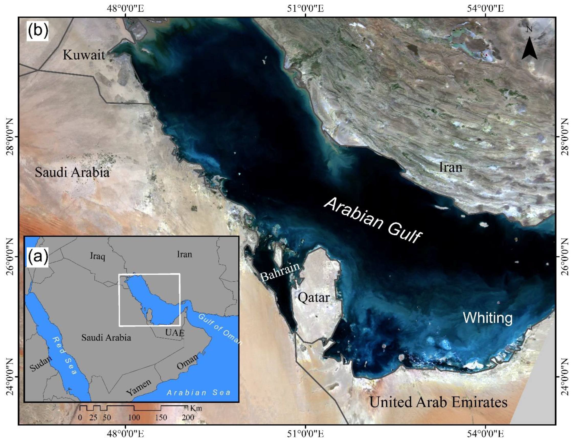
1.2. Study Region
2. Methodology
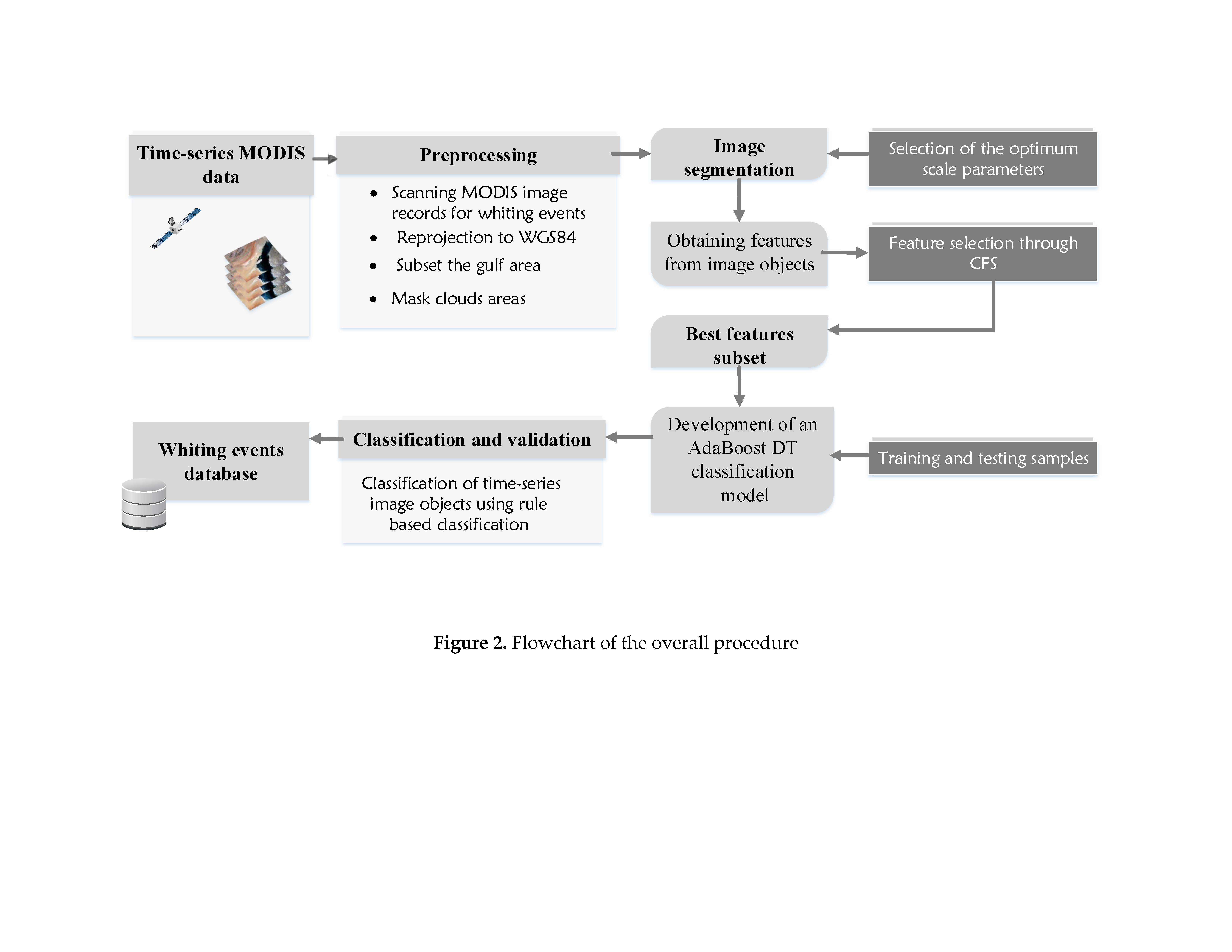
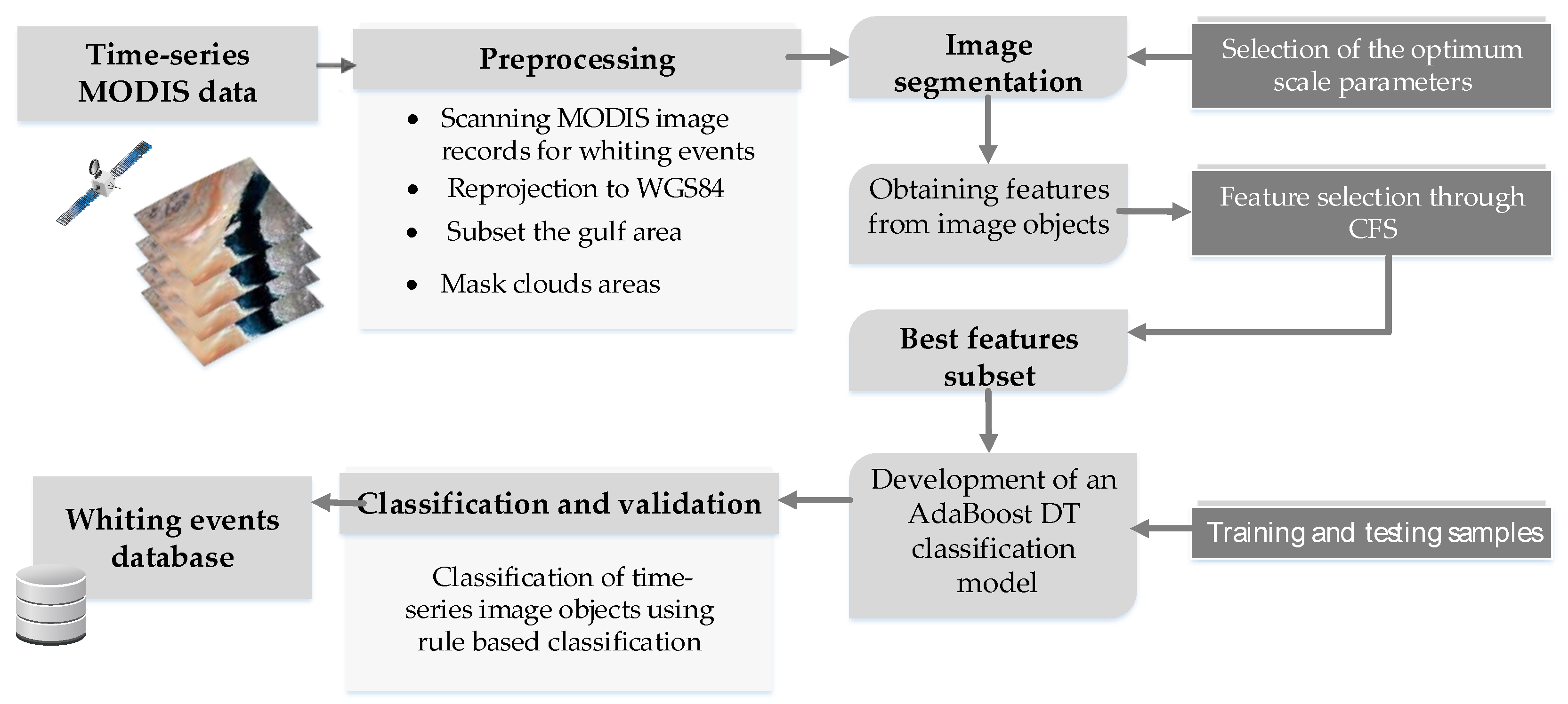
2.1. Overview
2.2. MODIS Datasets for Whiting Exploration
2.3. Object-Based Analysis and Image Segmentation Optimisation
2.4. Feature Selection
2.4.1. CFS
2.4.2. Feature Acquisition and Computation
2.5. Boosting Decision Tree Classification
3. Results & Discussion
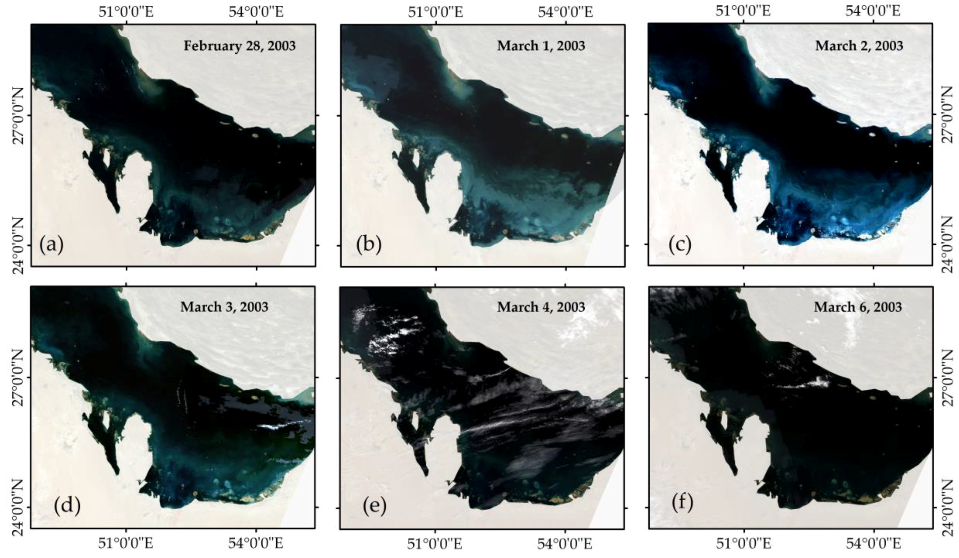
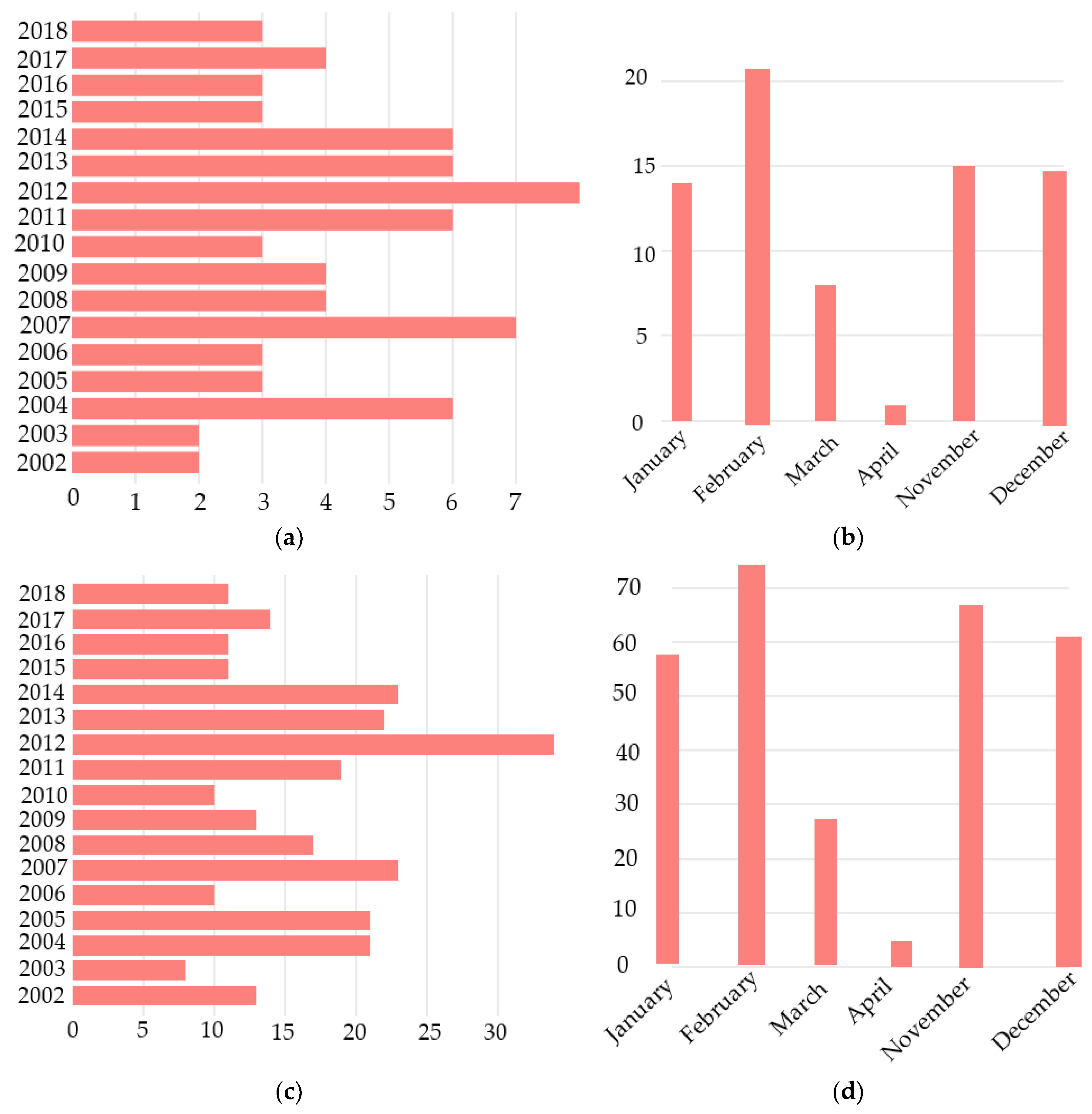
3.1. Whiting Temporal Pattern in the Gulf
3.2. Results of the Integrated GEOBIA Approach
3.2.1. Results of Image Segmentation
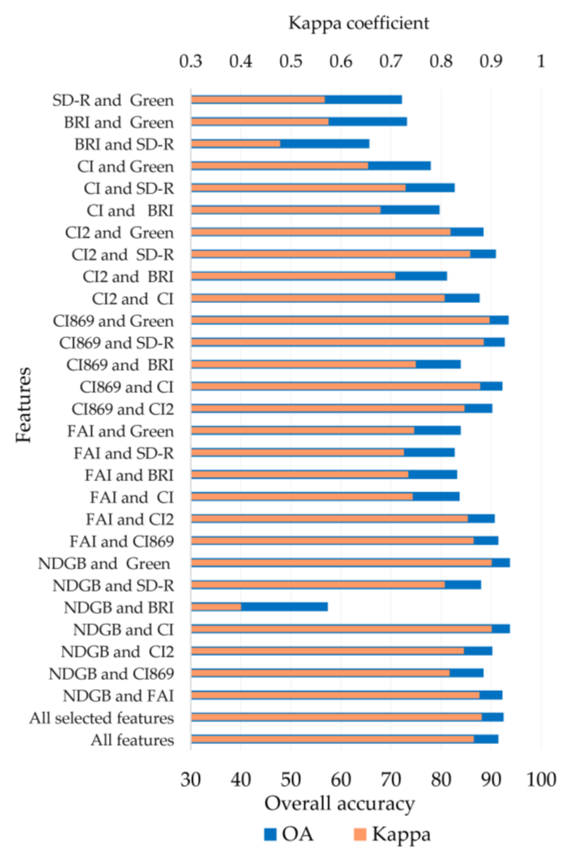
3.2.2. Results of FS and Analysis
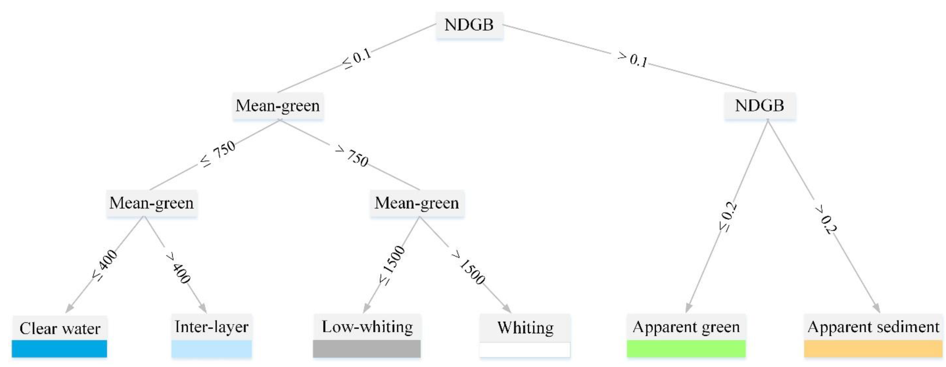
3.2.3. Classification Results
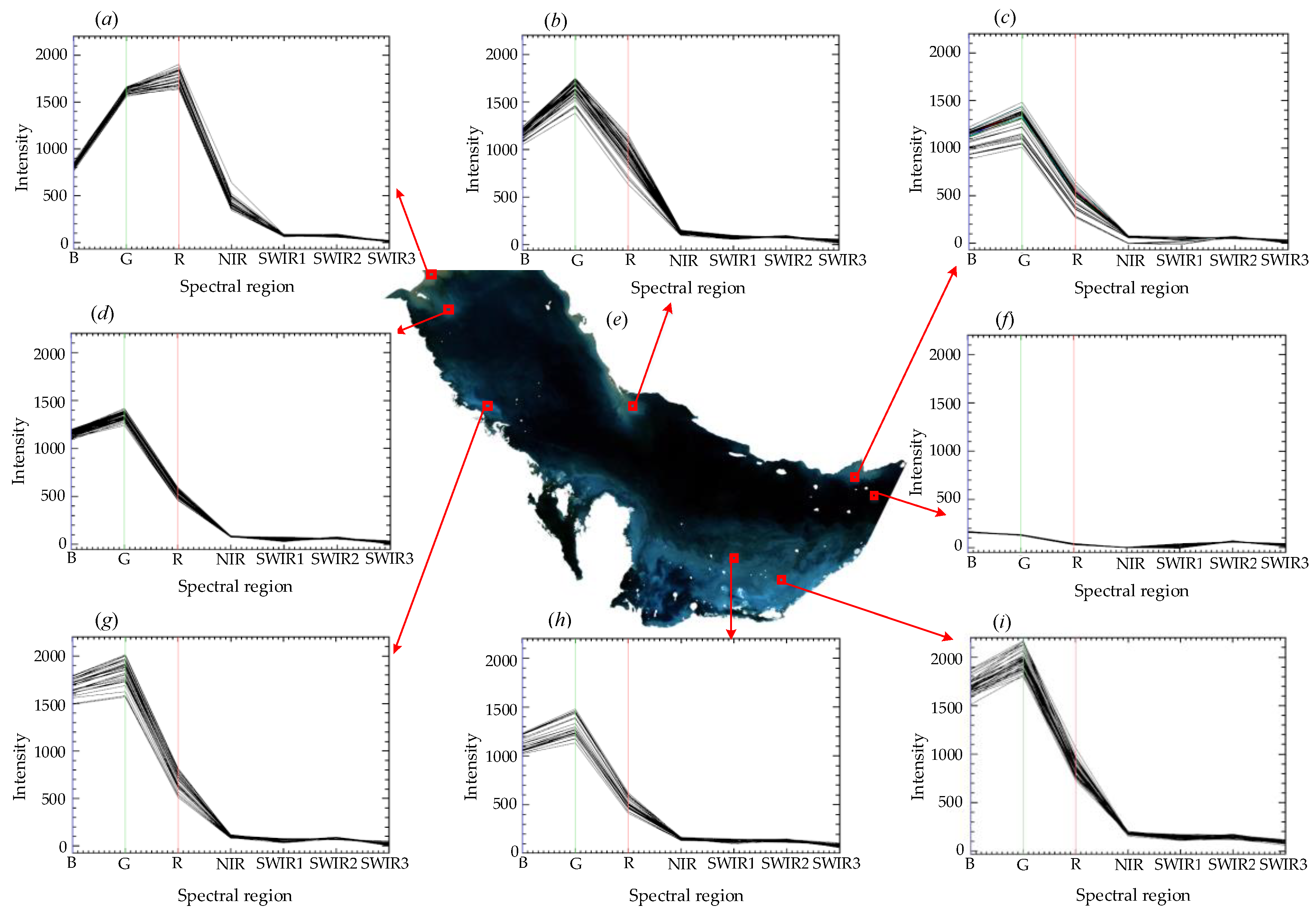
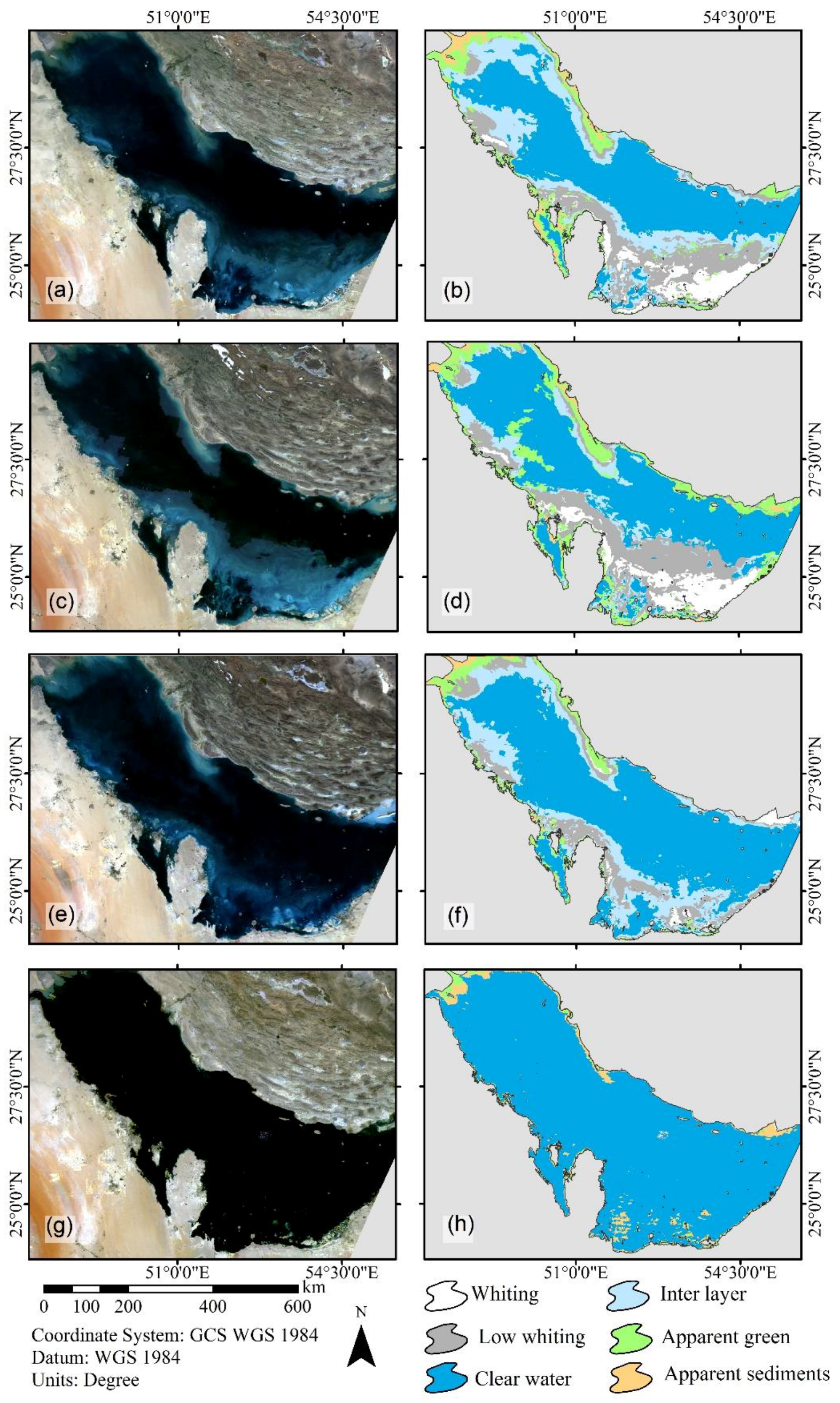
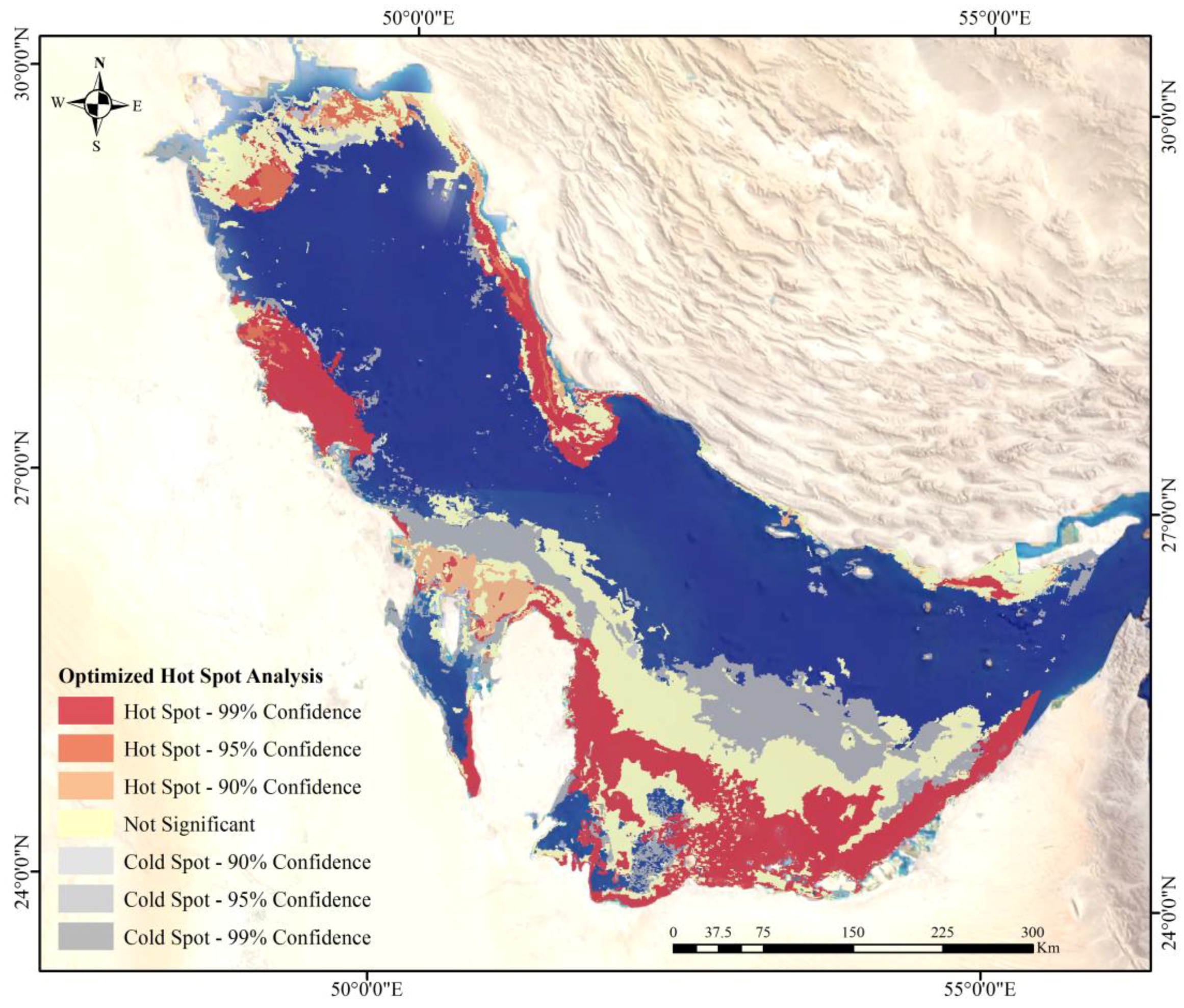
3.3. Spatial Distribution of Whiting in the Gulf
4. Conclusions
Author Contributions
Funding
Conflicts of Interest
References
- Long, J.S.; Hu, C.; Robbins, L.L.; Byrne, R.H.; Paul, J.H.; Wolny, J.L. Optical and biochemical properties of a southwest Florida whiting event. Estuar. Coast. Shelf Sci. 2017, 196, 258–268. [Google Scholar] [CrossRef]
- Morse, J.W.; He, S. Influence of T, S and PCO2 on the homogeneous nucleation of calcium carbonate from seawater. Implications for whiting formation. Mar. Chem. 1993, 41, 291–298. [Google Scholar] [CrossRef]
- Watkins, J.M.; Rudstam, L.G.; Crabtree, D.L.; Walsh, M.G. Is reduced benthic flux related to the Diporeia decline? Analysis of spring blooms and whiting events in Lake Ontario. J. Great Lakes Res. 2013, 39, 395–403. [Google Scholar] [CrossRef]
- Thompson, J.B.; Schultze-Lam, S.; Beveridge, T.J.; Des Marais, D.J. Whiting events: Biogenic origin due to the photosynthetic activity of cyanobacterial picoplankton. Limnol. Oceanogr. 1997, 42, 133–141. [Google Scholar] [CrossRef] [PubMed]
- Wurgaft, E.; Steiner, Z.; Luz, B.; Lazar, B. Evidence for Inorganic Precipitation of CaCO3 on Suspended Solids in the Open Water of the Red Sea. Mar. Chem. 2016, 186, 145–155. [Google Scholar] [CrossRef]
- Friedman, G.M. Biochemical and ultrastructural evidence for the origin of whitings: A biologically induced calcium carbonate precipitation mechanism: Comment and reply. Geology 1993, 21, 287–288. [Google Scholar] [CrossRef]
- Bloch, R.; Littman, H.Z.; Elazari-Volcani, B. Occasional whiteness of the dead sea. Nature 1944, 154, 402–403. [Google Scholar] [CrossRef]
- Bustos-Serrano, H.; Morse, J.W.; Millero, F.J. The formation of whitings on the Little Bahama Bank. Mar. Chem. 2009, 113, 1–8. [Google Scholar] [CrossRef]
- Bathurst, R.G.C. Carbonate Sediments and Their Diagenesis, 2nd ed.; Developments in Sedimentology; Elsevier: Amsterdam, The Netherlands, 1975; Volume 12, p. 658. [Google Scholar]
- Long, J.S.; Hu, C.; Wang, M. Long-term spatiotemporal variability of southwest Florida whiting events from MODIS observations. Int. J. Remote Sens. 2018, 39, 906–923. [Google Scholar] [CrossRef]
- Robbins, L.L.; Blackwelder, P.L. Biochemical and ultrastructural evidence for the origin of whiting: A biologically induced calcium carbonate precipitation mechanism. Geology 1992, 20, 464–468. [Google Scholar] [CrossRef]
- Dierssen, H.M.; Zimmerman, R.C.; Burdige, D.J. Optics and remote sensing of Bahamian carbonate sediment whitings and potential relationship to wind-driven Langmuir circulation. Biogeosciences 2009, 6, 487–500. [Google Scholar] [CrossRef] [Green Version]
- Broecker, W.S.; Takahashi, T. Calcium carbonate precipitation on the Bahama Banks. J. Geophys. Res. 1966, 71, 1575–1602. [Google Scholar] [CrossRef]
- Boss, S.K.; Neumann, A.C. Physical versus chemical processes of “whiting” formation in the Bahamas. Carbonates Evaporites 1993, 8, 135–148. [Google Scholar] [CrossRef]
- Shinn, E.A.; Steinen, R.P.; Lidz, B.H.; Swart, P.K. Whitings, a Sedimentologic Dilemma. J. Sediment. Petrol. 1989, 59, 147–161. [Google Scholar] [CrossRef]
- Cloud, P.E. Environment of Calcium Carbonate Deposition West of Andros Island Bahamas. Geol. Surv. Prof. Pap. 1962, 350, 170. [Google Scholar]
- Riding, R.E.; Awramik, S.M. Microbial Sediments; Springer: Berlin, Germany, 2000; ISBN 978-3-642-08275-7. [Google Scholar]
- Ohlendorf, C.; Sturm, M. Precipitation and Dissolution of Calcite in a Swiss High Alpine Lake. Arctic Antarct. Alp. Res. 2001, 33, 410–417. [Google Scholar] [CrossRef]
- Otsuki, A.; Wetzel, R.G. Calcium and total alkalinity budgets and calcium carbonate precipitation of a small hard-water lake. Arch. Hydrobiol. 1974, 73, 14–30. [Google Scholar] [CrossRef]
- Morse, J.W.; Gledhill, D.K.; Millero, F.J. CaCO3 precipitation kinetics in waters from the Great Bahama Bank: Implications for the relationship between Bank hydrochemistry and whitings. Geochim. Cosmochim. Acta 2003, 67, 2819–2826. [Google Scholar] [CrossRef]
- Shinn, E.A.; Kendall, C.G.S.C. Back to the Future. Sediment. Rec. 2011, 9, 4–9. [Google Scholar] [CrossRef]
- Lidz, B.; Gibbons, H. Research on Whitings (Floating Patches of Calcium Carbonate Mud) Leads to Possible Explanation of Immense Middle East Oil Deposits. Available online: https://soundwaves.usgs.gov/2008/07/research.html (accessed on 30 September 2018).
- Whitton, B.A. Ecology of Cyanobacteria II: Their Diversity in Space and Time; Springer: Dordrecht, The Netherlands, 2012; ISBN 978-94-007-3854-6. [Google Scholar]
- Robbins, L.L.; Tao, Y.; Evans, C.A. Temporal and spatial distribution of whitings on Great Bahama Bank and a new lime mud budget. Geology 1997, 25, 947–950. [Google Scholar] [CrossRef]
- Long, J.; Hu, C.; Robbins, L. Whiting events in SW Florida coastal waters: A case study using MODIS medium-resolution data. Remote Sens. Lett. 2014, 5, 539–547. [Google Scholar] [CrossRef]
- Strong, A.E.; Eadie, B.J. Satellite observations of calcium carbonate precipitation in the Great Lakes. Limnol. Ocean. 1978, 23, 877–887. [Google Scholar] [CrossRef]
- Heine, I.; Brauer, A.; Heim, B.; Itzerott, S.; Kasprzak, P.; Kienel, U.; Kleinschmit, B. Monitoring of calcite precipitation in hardwater lakes with multi-spectral remote sensing archives. Water 2017, 9, 15. [Google Scholar] [CrossRef]
- Millero, J. The carbonate chemistry of grand bahama bank waters: After 18 years another look. J. Geophys. Res. 1984, 89, 3604–3614. [Google Scholar]
- Long, J.S. Whiting Events Off Southwest Florida: Remote Sensing and Field Observations. Ph.D. Dissertation, University of South Florida, Tampa, FL, USA, 2016. [Google Scholar]
- Lloyd, R.A. Remote Sensing of Whitings in the Bahamas. Master’s Thesis, University of South Florida, Tampa, FL, USA, 2012. [Google Scholar]
- Tao, Y. Whitings on the Great Bahama Bank: Distribution in Space and Time Using Space Shuttle Photographs. Ph.D. Dissertation, University of South Florida, Tampa, FL, USA, 1994. [Google Scholar]
- Balch, W.M.; Gordon, H.R.; Bowler, B.C.; Drapeau, D.T.; Booth, E.S. Calcium carbonate measurements in the surface global ocean based on Moderate-Resolution Imaging Spectroradiometer data. J. Geophys. Res. C Ocean. 2005, 110, 1–21. [Google Scholar] [CrossRef]
- Gordon, R.; Boynton, G.C.; Balch, W.M.; Harbour, D.S.; Smyth, T.J.; Bay, W.B. Retrieval of Coccolithophore from SeaWiFS Imagery Calcite Concentration radiance. Geophys. Res. Lett. 2001, 28, 1587–1590. [Google Scholar] [CrossRef]
- Mitchell, C.; Hu, C.; Bowler, B.; Drapeau, D.; Balch, W.M. Estimating Particulate Inorganic Carbon Concentrations of the Global Ocean From Ocean Color Measurements Using a Reflectance Difference Approach. J. Geophys. Res. Ocean. 2017, 122, 8707–8720. [Google Scholar] [CrossRef]
- Wells, A.J.; Illing, L.V. Present-day precipitation of calcium carbonate in the Persian Gulf. Dev. Sedimentol. 1964, 1, 429–435. [Google Scholar] [CrossRef]
- Shanableh, A.; Imteaz, M.; Hamad, K.; Omar, M.; Merabtene, T.; Siddique, M. Potential impact of global warming on whiting in a semi-enclosed gulf. Int. J. Glob. Warm. 2017, 13, 411–425. [Google Scholar]
- Shanableh, A.; Al-Ruzouq, R.; Al-Khayyat, G. Assessing the Spatial and Temporal Capacity of a Semi-Enclosed Gulf to Absorb and Release CO2 Using GIS and Remote Sensing. In Proceedings of the Global Civil Engineering Conference, Kuala Lumpur, Malaysia, 25–28 July 2017; pp. 1161–1173. [Google Scholar]
- Sheppard, C.; Al-Husiani, M.; Al-Jamali, F.; Al-Yamani, F.; Baldwin, R.; Bishop, J.; Benzoni, F.; Dutrieux, E.; Dulvy, N.K.; Durvasula, S.R.V.; et al. Environmental Concerns for the Future of Gulf Coral Reefs; Springer: Dordrecht, The Netherlands, 2012; p. E1. ISBN 978-94-007-3007-6. [Google Scholar]
- Kaempf, J.; Sadrinasab, M. The circualtion of the Persian Gulf: A numerical study. Ocean Sci. 2006, 2, 27–41. [Google Scholar] [CrossRef]
- Ben-Hasan, A.; Walters, C.; Christensen, V.; Al-Husaini, M.; Al-Foudari, H. Is reduced freshwater flow in Tigris-Euphrates rivers driving fish recruitment changes in the Northwestern Arabian Gulf? Mar. Pollut. Bull. 2018, 129, 1–7. [Google Scholar] [CrossRef] [PubMed]
- Blaschke, T.; Hay, G.J.; Kelly, M.; Lang, S.; Hofmann, P.; Addink, E.; Queiroz Feitosa, R.; van der Meer, F.; van der Werff, H.; van Coillie, F.; et al. Geographic Object-Based Image Analysis—Towards a new paradigm. ISPRS J. Photogramm. Remote Sens. 2014, 87, 180–191. [Google Scholar] [CrossRef]
- Makinde, E.O.; Salami, A.T.; Olaleye, J.B.; Okewusi, O.C. Object Based and Pixel Based Classification Using Rapideye Satellite Imager of ETI-OSA, Lagos, Nigeria. Geoinform. FCE CTU 2016, 15, 59. [Google Scholar] [CrossRef]
- Petropoulos, G.P.; Vadrevu, K.P.; Kalaitzidis, C. Spectral angle mapper and object-based classification combined with hyperspectral remote sensing imagery for obtaining land use/cover mapping in a Mediterranean region. Geocarto Int. 2013, 28, 114–129. [Google Scholar] [CrossRef]
- da Silva Junior, C.A.; Nanni, M.R.; de Oliveira-Júnior, J.F.; Cezar, E.; Teodoro, P.E.; Delgado, R.C.; Shiratsuchi, L.S.; Shakir, M.; Chicati, M.L. Object-based image analysis supported by data mining to discriminate large areas of soybean. Int. J. Digit. Earth 2019, 12, 270–292. [Google Scholar] [CrossRef]
- Bisquert, M.; Bégué, A.; Deshayes, M. Object-based delineation of homogeneous landscape units at regional scale based on modis time series. Int. J. Appl. Earth Obs. Geoinf. 2015, 37, 72–82. [Google Scholar] [CrossRef]
- Cano, E.; Denux, J.P.; Bisquert, M.; Hubert-Moy, L.; Chéret, V. Improved forest-cover mapping based on MODIS time series and landscape stratification. Int. J. Remote Sens. 2017, 38, 1865–1888. [Google Scholar] [CrossRef]
- Vintrou, E.; Desbrosse, A.; Bégué, A.; Traoré, S.; Baron, C.; Lo Seen, D. Crop area mapping in West Africa using landscape stratification of MODIS time series and comparison with existing global land products. Int. J. Appl. Earth Obs. Geoinf. 2012, 14, 83–93. [Google Scholar] [CrossRef]
- Bontemps, S.; Bogaert, P.; Titeux, N.; Defourny, P. An object-based change detection method accounting for temporal dependences in time series with medium to coarse spatial resolution. Remote Sens. Environ. 2008, 112, 3181–3191. [Google Scholar] [CrossRef]
- Bisquert, M.; Bégué, A.; Deshayes, M.; Ducrot, D. Environmental evaluation of MODIS-derived land units. GISci. Remote Sens. 2017, 54, 64–77. [Google Scholar] [CrossRef]
- Bellón, B.; Bégué, A.; Lo Seen, D.; de Almeida, C.A.; Simões, M. A remote sensing approach for regional-scale mapping of agricultural land-use systems based on NDVI time series. Remote Sens. 2017, 9, 600. [Google Scholar] [CrossRef]
- Kim, M.; Madden, M.; Warner, T.T. Forest Type Mapping using Object-specific Texture Measures from Multispectral Ikonos Imagery: Segmentation Quality and Image Classification Issues. Photogramm. Eng. Remote Sens. 2009, 75, 819–829. [Google Scholar] [CrossRef]
- Baatz, M.; Sch, A. Multiresolution Segmentation: An optimization approach for high quality multi-scale image segmentation. J. Photogramm. Remote Sens. 2004, 58, 239–258. [Google Scholar]
- Grybas, H.; Melendy, L.; Congalton, R.G. A comparison of unsupervised segmentation parameter optimization approaches using moderate- and high-resolution imagery. GISci. Remote Sens. 2017, 54, 515–533. [Google Scholar] [CrossRef]
- Kim, M.; Warner, T.A.; Madden, M.; Atkinson, D.S. Multi-scale GEOBIA with very high spatial resolution digital aerial imagery: Scale, texture and image objects. Int. J. Remote Sens. 2011, 32, 2825–2850. [Google Scholar] [CrossRef]
- Hussain, M.; Chen, D.; Cheng, A.; Wei, H.; Stanley, D. Change detection from remotely sensed images: From pixel-based to object-based approaches. ISPRS J. Photogramm. Remote Sens. 2013, 80, 91–106. [Google Scholar] [CrossRef]
- Gao, Y.; Mas, J.F.; Kerle, N.; Pacheco, J.A.N. Optimal region growing segmentation and its effect on classification accuracy. Int. J. Remote Sens. 2011, 32, 3747–3763. [Google Scholar] [CrossRef]
- Johnson, B.; Bragais, M.; Endo, I.; Magcale-Macandog, D.; Macandog, P. Image Segmentation Parameter Optimization Considering Within- and Between-Segment Heterogeneity at Multiple Scale Levels: Test Case for Mapping Residential Areas Using Landsat Imagery. ISPRS Int. J. Geo-Inf. 2015, 4, 2292–2305. [Google Scholar] [CrossRef] [Green Version]
- Drǎguţ, L.; Csillik, O.; Eisank, C.; Tiede, D. Automated parameterisation for multi-scale image segmentation on multiple layers. ISPRS J. Photogramm. Remote Sens. 2014, 88, 119–127. [Google Scholar] [CrossRef] [Green Version]
- Zhang, X.; Xiao, P.; Feng, X. An unsupervised evaluation method for remotely sensed imagery segmentation. IEEE Geosci. Remote Sens. Lett. 2012, 9, 156–160. [Google Scholar] [CrossRef]
- Espindola, G.M.; Camara, G.; Reis, I.A.; Bins, L.S.; Monteiro, A.M. Parameter selection for region-growing image segmentation algorithms using spatial autocorrelation. Int. J. Remote Sens. 2006, 27, 3035–3040. [Google Scholar] [CrossRef]
- Laliberte, A.S.; Browning, D.M.; Rango, A. A comparison of three feature selection methods for object-based classification of sub-decimeter resolution UltraCam-L imagery. Int. J. Appl. Earth Obs. Geoinf. 2012, 15, 70–78. [Google Scholar] [CrossRef]
- Ma, L.; Cheng, L.; Li, M.; Liu, Y.; Ma, X. Training set size, scale, and features in Geographic Object-Based Image Analysis of very high resolution unmanned aerial vehicle imagery. ISPRS J. Photogramm. Remote Sens. 2015. [Google Scholar] [CrossRef]
- Al-Ruzouq, R.; Shanableh, A.; Barakat, A.; Gibril, M.; AL-Mansoori, S. Image Segmentation Parameter Selection and Ant Colony Optimization for Date Palm Tree Detection and Mapping from Very-High-Spatial-Resolution Aerial Imagery. Remote Sens. 2018, 10, 1413. [Google Scholar] [CrossRef]
- Georganos, S.; Grippa, T.; Vanhuysse, S.; Lennert, M.; Shimoni, M.; Kalogirou, S.; Wolff, E. Less is more: Optimizing classification performance through feature selection in a very-high-resolution remote sensing object-based urban application. GISci. Remote Sens. 2018, 55, 221–242. [Google Scholar] [CrossRef]
- Zhou, Y.; Chen, Y.; Feng, L.; Zhang, X.; Shen, Z.; Zhou, X. Supervised and Adaptive Feature Weighting for Object-Based Classification on Satellite Images. IEEE J. Sel. Top. Appl. Earth Obs. Remote Sens. 2018, 11, 3224–3234. [Google Scholar] [CrossRef]
- Benediktsson, J.A.; Pesaresi, M.; Arnason, K. Classification and feature extraction for remote sensing images from urban areas based on morphological transformations. IEEE Trans. Geosci. Remote Sens. 2003, 41, 1940–1949. [Google Scholar] [CrossRef] [Green Version]
- Dash, M.; Liu, H. Feature selection for classification. Intell. Data Anal. 1997, 1, 131–156. [Google Scholar] [CrossRef]
- Löw, F.; Michel, U.; Dech, S.; Conrad, C. Impact of feature selection on the accuracy and spatial uncertainty of per-field crop classification using Support Vector Machines. ISPRS J. Photogramm. Remote Sens. 2013, 85, 102–119. [Google Scholar] [CrossRef]
- Guyon, I.; Elisseeff, A. An introduction to variable and feature selection. J. Mach. Learn. Res. 2003, 3, 1157–1182. [Google Scholar]
- Duro, D.C.; Franklin, S.E.; Dubé, M.G. Multi-scale object-based image analysis and feature selection of multi-sensor earth observation imagery using random forests. Int. J. Remote Sens. 2012, 33, 4502–4526. [Google Scholar] [CrossRef]
- Hu, M.; Wu, F. Filter-wrapper hybrid method on feature selection. In Proceedings of the 2010 Second WRI Global Congress on Intelligent Systems, Wuhan, China, 16–17 December 2010; pp. 98–101. [Google Scholar] [CrossRef]
- Ma, L.; Fu, T.; Blaschke, T.; Li, M.; Tiede, D.; Zhou, Z.; Ma, X.; Chen, D. Evaluation of Feature Selection Methods for Object-Based Land Cover Mapping of Unmanned Aerial Vehicle Imagery Using Random Forest and Support Vector Machine Classifiers. ISPRS Int. J. Geo-Inf. 2017, 6, 51. [Google Scholar] [CrossRef]
- Gumus, E.; Kirci, P. Selection of spectral features for land cover type classification. Expert Syst. Appl. 2018, 102, 27–35. [Google Scholar] [CrossRef]
- Hamedianfar, A.; Barakat, A.M. Gibril Large-scale urban mapping using integrated geographic object-based image analysis and artificial bee colony optimization from worldview-3 data. Int. J. Remote Sens. 2019. [Google Scholar] [CrossRef]
- Ridha, M.; Pradhan, B. Catena An improved algorithm for identifying shallow and deep-seated landslides in dense tropical forest from airborne laser scanning data. Catena 2018, 167, 147–159. [Google Scholar] [CrossRef]
- Hall, M.A.; Smith, L.A. Feature subset selection: A correlation based filter approach. In International Conference on Neural Information Processing and Intelligent Information Systems; Springer: Berlin, Germany, 1997; pp. 855–858. [Google Scholar]
- Hall, M.A. Correlation-based feature selection of discrete and numeric class machine learning. In Proceedings of the 17th International Conference on Machine Learning, San Francisco, CA, USA, 29 June–2 July 2000; pp. 359–366. [Google Scholar]
- Hall, M.A.; Smith, L.A. Practical feature subset selection for machine learning. In Proceedings of the 21st Australasian Computer Science Conference ACSC’98, Perth, Australia, 4–6 February 1998; Volume 98, pp. 181–191. [Google Scholar]
- Hall, M.A.; Holmes, G. Benchmarking Attribute Selection Techniques for Discrete Class Data Mining. IEEE Trans. Knowl. Data Eng. 2003, 15, 1437–1447. [Google Scholar] [CrossRef]
- Trimble, T. ECognition Developer 8.7 Reference Book; Trimble Germany GmbH: Munich, Germany, 2011; pp. 319–328. [Google Scholar]
- Curran, P. Multispectral remote sensing of vegetation amount. Prog. Phys. Geogr. 1980, 4, 315–341. [Google Scholar] [CrossRef]
- Mcfeeters, S.K. The use of the Normalized Difference Water Index ( NDWI ) in the delineation of open water features. Int. J. Remote Sens. 1996, 17, 1425–1432. [Google Scholar] [CrossRef]
- Xu, H. Modification of normalised difference water index (NDWI) to enhance open water features in remotely sensed imagery. Int. J. Remote Sens. 2006, 27, 3025–3033. [Google Scholar] [CrossRef]
- Hu, C. A novel ocean color index to detect floating algae in the global oceans. Remote Sens. Environ. 2009, 113, 2118–2129. [Google Scholar] [CrossRef]
- Hu, C.; Lee, Z.; Franz, B. Chlorophyll a algorithms for oligotrophic oceans: A novel approach based on three-band reflectance difference. J. Geophys. Res. Ocean. 2012, 117, 1–25. [Google Scholar] [CrossRef]
- Xue, K.; Zhang, Y.; Duan, H.; Ma, R.; Loiselle, S.; Zhang, M. A remote sensing approach to estimate vertical profile classes of phytoplankton in a Eutrophic lake. Remote Sens. 2015, 7, 14403–14427. [Google Scholar] [CrossRef]
- Fensholt, R.; Sandholt, I. Derivation of a shortwave infrared water stress index from MODIS near- and shortwave infrared data in a semiarid environment. Remote Sens. Environ. 2003, 87, 111–121. [Google Scholar] [CrossRef]
- Jordan, C.F. Derivation of Leaf-Area Index from Quality of Light on the Forest Floor. Ecology 1969, 50, 663–666. [Google Scholar] [CrossRef]
- Huete, A.; Didan, K.; Miura, T.; Rodriguez, E.P.; Gao, X.; Ferreira, L.G. Overview of the radiometric and biophysical performance of the MODIS vegetation indices. Remote Sens. Environ. 2002, 83, 195–213. [Google Scholar] [CrossRef]
- Tucker, C.J. Red and photographic infrared linear combinations for monitoring vegetation. Remote Sens. Environ. 1979, 8, 127–150. [Google Scholar] [CrossRef] [Green Version]
- Zarco-Tejada, P.J.; Berjón, A.; López-Lozano, R.; Miller, J.R.; Martín, P.; Cachorro, V.; González, M.R.; De Frutos, A. Assessing vineyard condition with hyperspectral indices: Leaf and canopy reflectance simulation in a row-structured discontinuous canopy. Remote Sens. Environ. 2005, 99, 271–287. [Google Scholar] [CrossRef]
- Freund, Y.; Schapire, R.E. A Decision-Theoretic Generalization of On-Line Learning and an Application to Boosting. J. Comput. Syst. Sci. 1997, 55, 119–139. [Google Scholar] [CrossRef] [Green Version]
- Friedl, M.A.; McIver, D.K.; Hodges, J.C.F.; Zhang, X.Y.; Muchoney, D.; Strahler, A.H.; Woodcock, C.E.; Gopal, S.; Schneider, A.; Cooper, A.; et al. Global land cover mapping from MODIS: Algorithms and early results. Remote Sens. Environ. 2002, 83, 287–302. [Google Scholar] [CrossRef]
- DeFries, R. Multiple Criteria for Evaluating Machine Learning Algorithms for Land Cover Classification from Satellite Data. Remote Sens. Environ. 2000, 74, 503–515. [Google Scholar] [CrossRef]
- Zhou, Z.; Huang, J.; Wang, J.; Zhang, K.; Kuang, Z.; Zhong, S.; Song, X. Object-oriented classification of sugarcane using time-series middle-resolution remote sensing data based on AdaBoost. PLoS ONE 2015, 10, e0142069. [Google Scholar] [CrossRef] [PubMed]
- Maxwell, A.E.; Warner, T.A.; Fang, F. Implementation of machine-learning classification in remote sensing: An applied review. Int. J. Remote Sens. 2018, 39, 2784–2817. [Google Scholar] [CrossRef]
- Congalton, R.G.; Green, K. Assessing the Accuracy of Remotely Sensed Data: Principles and Practices, 2nd ed.; CRC Press, Taylor & Francis Group: Boca Raton, FL, USA, 2009; p. 183. ISBN 978-1-4200-5512-2. [Google Scholar]
- Xu, L.; Yan, P.; Chang, T. Best first strategy for feature selection. In Proceedings of the 9th International Conference on Pattern Recognition, Rome, Italy, 14 May–17 November 1988; pp. 706–708. [Google Scholar]
- Cheng, Z.; Zu, Z.; Lu, J. Traffic crash evolution characteristic analysis and spatiotemporal hotspot identification of urban road intersections. Sustainability 2018, 11, 161. [Google Scholar] [CrossRef]
- Al-Ruzouq, R.; Hamad, K.; Abu Dabous, S.; Zeiada, W.; Khalil, M.A.; Voigt, T. Weighted Multi-attribute Framework to Identify Freeway Incident Hot Spots in a Spatiotemporal Context. Arab. J. Sci. Eng. 2019. [Google Scholar] [CrossRef]


| No. | Examined Feature Name | Abbreviations | Description | MODIS Bands | Ref. |
|---|---|---|---|---|---|
| 1–7 | Mean values of an image object of MODIS reflectance (ref.) bands | Ref. 1–7 | Mean of bands 1–7 (Red, NIR, Blue, Green, SWIR1, SWIR2 and SWIR3) | B1–B7 | [80] |
| 8–14 | Standard deviation of an image object of ref. bands | SD 1–7 | Standard deviations of individual bands 1–7 | B1–B7 | [80] |
| 15 | Normalised difference vegetation index | NDVI | B2, B1 | [81] | |
| 16 | Normalised difference water index | NDWI | B4, B2 | [82] | |
| 17 | Modified normalised difference water index | MNDWI | B4, B7 | [83] | |
| 18 | Floating algae index | FAI | B1, B2, B5 | [84] | |
| 19 | Color index for estimating PIC | CI | B1, B3, B4 | [85] | |
| 20 | Color index using 547, 667 and 869 nm for estimating PIC | CI869 | B1, B2, B4 | [34] | |
| 21 | Color index using 547 and 667 nm for estimating PIC | CI2 | B1, B4 | [34] | |
| 22 | Normalised difference algal bloom index | NDBI | B4, B1 | [86] | |
| 23 | Shortwave infrared water stress index | SIWS | B6, B2 | [87] | |
| 24 | Ratio vegetation index 1 | RVI 1 | B2, B1 | [88] | |
| 25 | Ratio vegetation index 2 | RVI 2 | B1, B2 | [88] | |
| 26 | Enhanced vegetation index | EVI | 2.5 | B2, B1, B3 | [89] |
| 27 | Ratio of the reflectance values of red and green bands | Ratio RG | B1, B4 | [90] | |
| 28 | Blue/red index | BRI | B3, B1 | [91] | |
| 29 | Blue/green index | BGI | B3, B4 | [91] | |
| 30 | Normalised difference between green and red bands | NDGR | B4, B1 | - | |
| 31 | Normalised difference between green and blue bands | NDGB | B4, B3 | - | |
| 32 | Normalised difference between blue and green bands | NDBG | B3, B4 | - |
| Dates | Whiting Samples | Clear Water | Other Segments |
|---|---|---|---|
| 28 February 2003 | 74 | 149 | 74 |
| 2 March 2003 | 100 | 125 | 126 |
| 3 March 2003 | 121 | 36 | 74 |
| 26 February 2004 | 69 | 124 | 66 |
| 2 February 2018 | 36 | 160 | 72 |
| Sum | 400 | 594 | 412 |
| Year | Month | Dates | Period (d) | Frequency Event | Year | Month | Dates | Period (d) | Frequency Event |
|---|---|---|---|---|---|---|---|---|---|
| 2002 | February | 1–5 | 5 | 1 | November | 10–11 | 2 | 2 | |
| December | 23–30 | 8 | 1 | November | 24–25 | 2 | |||
| 2003 | February | 28–1 | 2 | - | December | 1–6 | 6 | 2 | |
| March | 1–3 | 3 | 1 | December | 27–30 | 4 | |||
| December | 9–11 | 3 | 1 | 2012 | January | 15–16 | 2 | 2 | |
| 2004 | January | 29–31 | 3 | 1 | January | 21–26 | 6 | ||
| February | 7–10 | 4 | 3 | February | 3–7 | 5 | 2 | ||
| February | 16–17 | 2 | February | 21–24 | 4 | ||||
| February | 25–27 | 3 | March | 4–13 | 10 | 2 | |||
| March | 21–23 | 3 | 1 | March | 18–19 | 2 | |||
| November | 24–29 | 6 | 1 | November | 2–3 | 2 | 2 | ||
| 2005 | February | 10–11 | 2 | 1 | November | 12–14 | 3 | ||
| November | 1–11 | 11 | 2 | 2013 | January | 11–18 | 8 | 1 | |
| November | 24–31 | 8 | February | 4–5 | 2 | 2 | |||
| 2006 | January | 15–20 | 6 | 1 | February | 14–15 | 2 | ||
| December | 9–10 | 2 | 2 | March | 12–13 | 2 | 1 | ||
| December | 25–26 | 2 | December | 11–18 | 8 | 2 | |||
| 2007 | January | 1–4 | 4 | 1 | December | 20–27 | 8 | ||
| March | 4–5 | 2 | 2 | 2014 | February | 11–13 | 3 | 2 | |
| March | 11–13 | 3 | February | 19–21 | 3 | ||||
| April | 19–21 | 3 | 1 | November | 7–10 | 4 | 2 | ||
| November | 25–30 | 6 | 1 | November | 26–30 | 5 | |||
| December | 11–13 | 3 | 2 | December | 2–7 | 6 | 2 | ||
| December | 24–25 | 2 | December | 25–26 | 2 | ||||
| 2008 | February | 3–7 | 5 | 2 | 2015 | January | 19–24 | 6 | 1 |
| February | 21–27 | 7 | February | 27–28 | 2 | 1 | |||
| March | 6–7 | 2 | 1 | November | 13–15 | 3 | 1 | ||
| December | 17–19 | 3 | 1 | 2016 | Jan | 4–6 | 3 | 1 | |
| 2009 | January | 4–7 | 4 | 2 | Jan–Feb | 29–2 | 4 | 1 | |
| January | 14–16 | 3 | February | 10–13 | 4 | 1 | |||
| February | 3–6 | 4 | 1 | 2017 | February | 4–8 | 5 | 1 | |
| November | 7–8 | 2 | 1 | November | 10–14 | 5 | 2 | ||
| 2010 | January | 27–28 | 2 | 1 | November | 29–30 | 2 | ||
| November | 23–28 | 6 | 1 | December | 4–5 | 2 | 1 | ||
| December | 16–17 | 2 | 1 | 2018 | January | 2–5 | 4 | 1 | |
| 2011 | January | 12–14 | 3 | 1 | January | 29–31 | 3 | 1 | |
| February | 4–5 | 2 | 2 | February | 1–4 | 4 | 1 |
| SP | No. of Objects | Weighted Variance | Moran’s I | WV Norm | MI Norm | OF | F-Measure |
|---|---|---|---|---|---|---|---|
| 10 | 32,227 | 326.8510 | 0.4118 | 1 | 0 | 1 | 0 |
| 20 | 12,446 | 1012.3473 | 0.2597 | 0.8883 | 0.3747 | 1.2630 | 0.5271 |
| 30 | 6695 | 1784.3010 | 0.2013 | 0.7625 | 0.5187 | 1.2812 | 0.6174 |
| 40 | 4208 | 2606.2537 | 0.1425 | 0.6285 | 0.6636 | 1.2921 | 0.6456 |
| 50 | 2891 | 3394.2522 | 0.1022 | 0.5001 | 0.7630 | 1.2631 | 0.6042 |
| 60 | 2197 | 4173.2623 | 0.0789 | 0.3732 | 0.8204 | 1.1936 | 0.5130 |
| 70 | 1755 | 4780.7261 | 0.0485 | 0.2742 | 0.8953 | 1.1695 | 0.4198 |
| 80 | 1459 | 5468.1106 | 0.0316 | 0.1621 | 0.9370 | 1.0991 | 0.2764 |
| 90 | 1202 | 6039.1318 | 0.0178 | 0.0691 | 0.9708 | 1.0399 | 0.1290 |
| 100 | 1039 | 6463.0462 | 0.0060 | 0 | 1 | 1 | 0 |
| Classifier | OA | KC |
|---|---|---|
| AdaBoost DT | 97.86% | 0.97 |
| Gradient boosted DT | 97.12% | 0.96 |
| Single DT | 96.19% | 0.95 |
| Random forest | 95.00% | 0.93 |
| Year | Date | Whiting Area (km2) | Percentage of Gulf Area |
|---|---|---|---|
| 2002 | 5 February | 15,655 | 6.55 |
| 2003 | 2 March | 53,687 | 22.46 |
| 2004 | 9 February | 29,874 | 12.50 |
| 2005 | 6 April | 44,894 | 18.78 |
| 2006 | 30 January | 30,549 | 12.78 |
| 2007 | 11 December | 20,481 | 8.57 |
| 2008 | 22 February | 47,887 | 20.04 |
| 2009 | 5 February | 22,584 | 9.45 |
| 2010 | 16 December | 12,100 | 5.06 |
| 2011 | 5 December | 17,340 | 7.26 |
| 2012 | 4 March | 60,847 | 25.46 |
| 2013 | 4 February | 39,544 | 16.55 |
| 2014 | 10 November | 15,137 | 6.33 |
| 2015 | 15 November | 19,201 | 8.03 |
| 2016 | 10 February | 30,480 | 12.75 |
| 2017 | 6 January | 45,753 | 19.14 |
| 2018 | 3 February | 22,159 | 9.27 |
© 2019 by the authors. Licensee MDPI, Basel, Switzerland. This article is an open access article distributed under the terms and conditions of the Creative Commons Attribution (CC BY) license (http://creativecommons.org/licenses/by/4.0/).
Share and Cite
Shanableh, A.; Al-Ruzouq, R.; Gibril, M.B.A.; Flesia, C.; AL-Mansoori, S. Spatiotemporal Mapping and Monitoring of Whiting in the Semi-Enclosed Gulf Using Moderate Resolution Imaging Spectroradiometer (MODIS) Time Series Images and a Generic Ensemble Tree-Based Model. Remote Sens. 2019, 11, 1193. https://doi.org/10.3390/rs11101193
Shanableh A, Al-Ruzouq R, Gibril MBA, Flesia C, AL-Mansoori S. Spatiotemporal Mapping and Monitoring of Whiting in the Semi-Enclosed Gulf Using Moderate Resolution Imaging Spectroradiometer (MODIS) Time Series Images and a Generic Ensemble Tree-Based Model. Remote Sensing. 2019; 11(10):1193. https://doi.org/10.3390/rs11101193
Chicago/Turabian StyleShanableh, Abdallah, Rami Al-Ruzouq, Mohamed Barakat A. Gibril, Cristina Flesia, and Saeed AL-Mansoori. 2019. "Spatiotemporal Mapping and Monitoring of Whiting in the Semi-Enclosed Gulf Using Moderate Resolution Imaging Spectroradiometer (MODIS) Time Series Images and a Generic Ensemble Tree-Based Model" Remote Sensing 11, no. 10: 1193. https://doi.org/10.3390/rs11101193