A Comprehensive Evaluation of Approaches for Built-Up Area Extraction from Landsat OLI Images Using Massive Samples

1
Beijing Key Laboratory for Remote Sensing of Environment and Digital Cities, Faculty of Geographical Science, Beijing Normal University, Beijing 100875, China
2
State Key Laboratory of Remote Sensing Science, Jointly Sponsored by Beijing Normal University and Institute of Remote Sensing and Digital Earth of Chinese Academy of Sciences, Beijing 100875, China
*
Author to whom correspondence should be addressed.
Remote Sens. 2019, 11(1), 2; https://doi.org/10.3390/rs11010002
Submission received: 4 December 2018
/
Revised: 16 December 2018
/
Accepted: 17 December 2018
/
Published: 20 December 2018
(This article belongs to the Special Issue Remote Sensing for Urban Morphology)
Abstract
:Detailed information about built-up areas is valuable for mapping complex urban environments. Although a large number of classification algorithms for such areas have been developed, they are rarely tested from the perspective of feature engineering and feature learning. Therefore, we launched a unique investigation to provide a full test of the Operational Land Imager (OLI) imagery for 15-m resolution built-up area classification in 2015, in Beijing, China. Training a classifier requires many sample points, and we proposed a method based on the European Space Agency’s (ESA) 38-m global built-up area data of 2014, OpenStreetMap, and MOD13Q1-NDVI to achieve the rapid and automatic generation of a large number of sample points. Our aim was to examine the influence of a single pixel and image patch under traditional feature engineering and modern feature learning strategies. In feature engineering, we consider spectra, shape, and texture as the input features, and support vector machine (SVM), random forest (RF), and AdaBoost as the classification algorithms. In feature learning, the convolutional neural network (CNN) is used as the classification algorithm. In total, 26 built-up land cover maps were produced. The experimental results show the following: (1) The approaches based on feature learning are generally better than those based on feature engineering in terms of classification accuracy, and the performance of ensemble classifiers (e.g., RF) are comparable to that of CNN. Two-dimensional CNN and the 7-neighborhood RF have the highest classification accuracies at nearly 91%; (2) Overall, the classification effect and accuracy based on image patches are better than those based on single pixels. The features that can highlight the information of the target category (e.g., PanTex (texture-derived built-up presence index) and enhanced morphological building index (EMBI)) can help improve classification accuracy. The code and experimental results are available at https://github.com/zhangtao151820/CompareMethod.
1. Introduction
“Built-up area” refers to land used for urban and rural residential purposes and public facilities. Built-up areas are one of the most important elements of land use and play an extremely important role in urban development planning [1]. Extracting built-up areas is crucial for mapping and the management of complex urban environments across local and regional scales [2,3,4,5,6]. Landsat images, a good source of data for generating information about built-up areas over large areas, are frequently used for this purpose [7,8]. However, the mapping of built-up land poses a significant challenge for remote sensing due to the high spatial frequency and heterogeneity of surface features. Various algorithms have been applied to extract built-up areas, including supervised classification, unsupervised clustering, and reinforcement learning [9,10,11]. In the process of built-up area extraction, the most important considerations are how to design or learn better features to characterize the buildings and how to choose a more appropriate classification strategy. Li et al. [12] tested two unsupervised and 13 supervised classification algorithms to distinguish urban land in Guangzhou City and then assessed all the algorithms in a per-pixel classification decision experiment and all the supervised algorithms in a segment-based experiment. Momeni et al. [13] compared the influence of spatial resolution, spectral band set, and the classification approach for mapping detailed urban land cover in Nottingham, UK. A WorldView-2 image provides the basis for a set of 12 images with variable spatial and spectral characteristics within three different approaches, namely maximum likelihood (ML), support vector machine (SVM), and object-based image analysis (OBIA), to yield 36 output land cover maps. Lu and Weng [14] summarized the major advanced classification approaches and the techniques used for improving classification accuracy. Radar imagery, which uses active remote sensing to obtain information regarding surface objects, has the advantages of (1) not being affected by weather and (2) acquiring three-dimensional hierarchical information, and as a result, it has been used in the recognition of urban building. Xiang et al. [15,16,17] utilized polarimetric Synthetic Aperture Radar (PolSAR) imagery and proposed a multiple-component model-based decomposition method to identify urban buildings. Their experimental results demonstrated that the decomposed scattering powers and the proposed polarimetric coherence coefficient ratio are both capable of distinguishing urban areas from natural areas with an accuracy of about 83.1% and 80.1%, respectively. However, SAR images cannot be obtained conveniently in a wide range. It is impossible to classify large urban built-up areas by using only small-scale SAR datasets.
In this paper, we focused on the following three aspects: (1) In the large region of mapping built-up areas, Google Earth Engine (GEE) was used to obtain high-quality images; (2) using existing built-up area data products and open map data, a large number of samples were selected quickly and automatically, and the samples were then filtered and corrected; and (3) from the viewpoint of feature engineering and feature learning, the influence of the classification strategy and the features on the result of built-up area extraction was synthetically analyzed.
In the following sections, we review the methods and techniques of feature engineering and feature learning and the classification strategies based on single pixels and image patches. The application and advantages and disadvantages of these methods and techniques in built-up area extraction are discussed. We also discuss the progress and shortcomings of built-up area mapping based on low- and medium-resolution images.
1.1. Feature Engineering versus Feature Learning
A key step for pattern recognition and classification is to select independent and measurable features with a large amount of information, distinction, and independence. Feature engineering performs mathematical operations on the image to obtain the typical and specific features that can represent the extracted object. This is equivalent to the realization of feature transformation, mapping from the original image feature space to a new feature space after feature engineering. Different combinations of bands can highlight different surface features. The simplest feature transformation of remote sensing images is the band operation. The normalized difference building index (NDBI), an index-based built-up index (IBI), and a texture-derived built-up presence index (PanTex) were proposed to characterize buildings in [18,19,20]. However, these methods based on the remote sensing index have a strong dependence on threshold selection, and finding a suitable threshold is very difficult. In recent years, very high-resolution and hyperspectral images have been gradually used in building extraction. The texture, shape, geometry, and three-dimensional features of images have been applied to recognize and distinguish objects. Many methods based on morphological filtering [2], spatial structure features [3,21], grayscale texture features [4], image segmentation [5,22], geometric features [6,23,24], and three-dimensional modeling [25] have increasingly been applied to building extraction. Pattern classification based on feature engineering has a good advantage in extracting certain ground objects (vegetation and water). However, for the recognition and classification of built-up areas, because of the uneven distribution and fragmentation of buildings, large surface spectral heterogeneity, and morphological characteristics without a fixed pattern, it is difficult to find a suitable feature in a wide range of urban and suburban areas.
In recent years, with the rise of artificial intelligence and large data, pattern classification based on feature learning has become a popular research topic, especially in in-depth learning [9,10,11,26,27] and reinforcement learning [28,29,30,31,32,33]. Feature learning automatically learns and utilizes features from raw data. Deep learning (DL) can automatically extract hierarchical data features by unsupervised or semi-supervised feature-learning algorithms. In contrast, traditional machine learning methods require manual design features. DL is a representation learning algorithm based on large-scale data in machine learning. Modern DL methods have often been applied successfully in the field of feature learning, such as self-encoder [34], restricted Boltzmann machine [35], and generative adversarial networks [36]. These implement automatic learning abstract feature representation in an unsupervised or semi-supervised manner, and their results support advanced achievements in areas such as speech recognition, image classification [37], and object recognition [38]. With the rapid development of convolutional neural networks (CNNs), especially the excellent performance of deep CNNs on the ImageNet contest [39,40,41,42], CNNs have shown great advantages in image pattern recognition, scene classification [43], object detection, and other issues. An increasing number of researchers have applied CNN to remote sensing image classification. CNNs of different structures were used for building extraction in [44,45,46]. Yang et al. [47] showed that the combination of a subset of spectral bands can promote the classification accuracy of CNNs.
1.2. Pixel-Based versus Patch-Based Classification
With the improvement of image spatial resolution, the basic unit of remote sensing land cover mapping has undergone a transformation from image pixels to image objects (segments and patches). The goal of remote sensing land cover mapping is usually to obtain the semantic category of each pixel. Traditionally, built-up extraction has been conducted using pixel-based approaches, where land cover classes are allocated to each individual pixel. In a feature space, a classifier (e.g., SVM or k-nearest neighbors (KNN)) is used to separate the feature space into several regions. In the transformation of the feature space and the image plane space, there is the problem that the same object with different spectra and different objects can have the same spectrum, because the spatial relationship cannot be considered. Therefore, the classification results of the image plane will exhibit salt-and-pepper noise and fragmentation. Momeni et al. [13] compared the influence of spatial resolution, spectral band set, and the classification approach for mapping detailed urban land cover based on WorldView-2 images. Their results demonstrated that spatial resolution is clearly the most influential factor when mapping complex urban environments. Wang et al. [48] identified and inspected an urban built-up area boundary based on the temperature retrieval method and used qualitative and quantitative analysis methods to analyze the spatio-temporal characteristics of the expansion of the Jingzhou urban built-up area from 1990 to 2014.
With the improvement of image spatial resolution, and especially with the launch of the SPOT, QuickBird, and Worldview satellites, a large number of high-resolution images are now publicly available. High-resolution images, hyperspectral images, and radar data are widely used to extract built-up areas. Relying on single-pixel spectral information cannot adequately describe and reflect the feature information of ground objects. Instead of the pixels’ features, one might use image patches as the features of geo-objects. In one image patch, the spatial relations and semantic links between pixels are considered, regarding a patch as one or more target objects, such as scene recognition, semantic segmentation, and object detection. Zhong and Wang [7] presented a multiple conditional random fields (CRFs) ensemble model to incorporate multiple features and learn their contextual information; their experiments on a wide range of images showed that their ensemble model produces higher extraction accuracy for built-up areas than a single CRF. Ning and Lin [49] presented a method for extracting built-up areas from very high-resolution (VHR) remote sensing imagery using the feature-level-based fusion of right-angle corners, right-angle sides, and road marks. On average, the completeness and the quality of their proposed method are 17.94% and 13.33% better than those of the PanTex method, respectively.
1.3. Built-Up Area Extraction from Medium-Resolution Images
Although an increasing number of high-resolution images are available, medium-resolution images are still the most widely used for a wide range of ground object extractions, due to limited computer performance and considerable data mining technology. Worldwide, the spatial resolution of built-up area data ranges from low to high, with resolutions of 500, 250, 38, and 30 m. The International Geosphere Biosphere Programme (IGBP) scheme was classified using the C4.5 decision tree algorithm that ingested a full year of 8-day moderate-resolution imaging spectroradiometer (MODIS) Nadir Bidirectional Reflectance Distribution Function (BRDF)-adjusted reflectance data [50]. Schaaf et al. [8] utilized a random forest (RF) classification algorithm to map global land cover in 2001 and 2010 with spatial-temporal consistency based on MODIS data and Landsat images. Gong [51] produced the first 30-m resolution global land cover maps based on four classifiers (ML, J4.8 decision tree, RF, and SVM) using Landsat Thematic Mapper (TM) and Enhanced Thematic Mapper Plus (ETM+) data. Based on TM and ETM+ images, Chen et al. [52] applied the pixel-object hierarchical classification method to extract the global man-made surface, and the user accuracy reached 80%. Using the symbolic classification algorithm [53], the ESA processed massive Landsat images and high-resolution images to extract 38-m resolution global residential areas in 1975, 1990, 2000, and 2014, with an overall accuracy of more than 85%. Based on the GEE platform [54], Liu et al. proposed the urban comprehensive land use index [55] and found the appropriate threshold in the global sub-climate areas and extracted multi-temporal urban built-up areas [56].
In smaller regions, research on built-up area extraction methods has become a popular topic. For example, Zhang et al. [57] proposed an empirical normalized difference of a seasonal brightness temperature index (NDSTI) for enhancing a built-up area based on the contrast heat emission seasonal response of the area to solar radiation and adopted a decision tree classification method for the rapid and accurate extraction of the area. Goldblatt et al. [5] presented an efficient and low-cost machine-learning approach for the pixel-based image classification of built-up areas at a large geographic scale using Landsat data. Their methodology combines nighttime-light data and Landsat 8 images and overcomes the lack of extensive ground reference data. Ma et al. [58] presented a sample-optimized approach for classifying urban area data in several cities of western China using a combination of the Defense Meteorological Satellite Program (DMSP)- Operational Linescan System (OLS) for nighttime-light data, Landsat images, and GlobeLand30. Goldblatt et al. [59] applied a classification and regression tree, SVM, and RFs to extract urban areas in India based on a single pixel using the GEE platform.
In this paper, we compare the accuracy and efficiency of the approaches for built-up area extraction from Landsat 8-OLI images based on single pixels or image patches in two perspectives of feature engineering and feature learning. We systematically and comprehensively compare the impact of features and classifiers on built-up area extraction results using 15-m resolution OLI-images. Moreover, given the influential role that the classification approach plays on output accuracy and how this is linked intrinsically with image specifications, all the image datasets are classified using parametric and non-parametric pixel-based and patch-based classifiers. This enables a fuller and more robust assessment of the Landsat 8 data and transmits helpful and practical information for urban planners and other user communities on the level of thematic detail that can be achieved when mapping complex built-up areas. Finally, an analysis was conducted using a relatively large image covering approximately 32,400 km2 of the city of Beijing, China, and its surroundings. This means that built-up area extraction is generated at a scale of practical value and relevance (the whole city-scale), unlike the earlier experiments of Li et al. [12] and Momeni et al. [13], which were limited to very small local areas.
2. Study Site and Data
2.1. Study Area and OLI Image
The study area is the city of Beijing, the capital of China, which is located at 36°N latitude, 107°E longitude. Beijing has a population of slightly more than 21 million. The climate is a typical northern, temperate, semi-humid, continental monsoon climate, with a hot and rainy summer, a cold and dry winter, and a short spring and autumn. The landscape consists of 62% mountains and 38% plains. The topography of Beijing is high in the northwest and low in the southeast, with an average elevation of approximately 43.5 m. Beijing is a typical international metropolis with prosperous business circles and developed transportation systems. The objects on the ground surface are complex and heterogeneous. Within the Fifth Ring, the buildings are densely distributed, while the buildings are sparse in the suburbs outside the Fifth Ring. Therefore, we determined that choosing Beijing as an experimental area is typical, scientific, and reasonable.
The Landsat 8-OLI land imager has nine bands, and the imaging width is 185 × 185 km. The resolution of Bands 1–7 is 30 m, and Band 8 is a panchromatic band with a resolution of 15 m. Compared with the Enhanced Thematic Mapper Plus (ETM+) sensor on Landsat-7 (Table 1), the OLI terrestrial imager has made the following adjustments: (1) The wavelength of Band 5 is adjusted to 0.845–0.885 µm, thus eliminating the influence of water vapor absorption at 0.825 µm; (2) the Band 8 panchromatic wave band is narrow, so that vegetation and non-vegetation areas can be distinguished better; and (3) the newly added blue band of Band 1 (0.433–0.453 µm) is mainly used for the observation of coastal zones.
We selected OLI images on GEE; due to the large amount of cloud cover in spring and autumn, the images are mainly from summer. To ensure data quality, we utilized the minimum cloud cover synthesis algorithm provided by GEE to preprocess and generate the required images [54]. To facilitate the built-up area extraction at 15-m resolution, the first seven bands (Bands 1–7) of the Landsat 8 OLI images were up-sampled to 15 m using the nearest neighborhood sampling. We then clipped the image with a size of 12,000 × 12,000 pixels. As shown in Figure 1, the false color (combination of Bands 4, 6, and 7) showed that the quality of the data was good and met the requirements. To facilitate the mapping display and to more clearly express the details, we chose two representative regions, A and B, with sizes of 1000 × 1000 pixels. Region B is an urban central region with a dense distribution of buildings, while region A is a suburban region with a sparse distribution of buildings. However, we still considered the whole research area as the analysis object when conducting the experiment.
2.2. Massive Samples Automatically Selected from Built-Up Production
The training and testing samples were automatically selected from the 38-m global built-up production of the ESA in 2014 [53]. A large number of sample points were automatically generated, filtered, and corrected. As shown in Figure 2, the detailed process included three steps: (1) Randomly selecting 20,000 sample points in each experimental area; (2) using the buildings and water datasets of OpenStreetMap (OSM) in China and the MOD13Q1-NDVI data to filter and correct the selected sample points; and (3) combining with ArcGIS Online image for manual correction. The aim was to modify the built-up sample points in the vegetation area and the water body into non-built-up sample points and to modify the non-built-up sample points in the built-up area into the built-up sample points. Finally, sample points of the built-up area and non-built-up area were obtained. The sample points after filtration and correction were hierarchically divided into training samples and test samples at a proportion of 6:4. Finally, a total of 11,499 training samples and 7667 test samples were obtained. In Figure 1, the yellow points represent built-up samples and the blue points represent non-built-up samples.
3. Research Methods
In this paper, the accuracy and efficiency of extracting a 15-m resolution built-up area based on a single pixel and image patch were compared and analyzed comprehensively from the two perspectives of feature engineering and feature learning. As shown in Table 2, we proceeded based upon four classifications: (1) Single-pixel classification under feature engineering, that is, pre-set features using the original eight-band spectrum, building remote sensing indices (NDBI and IBI), enhanced morphological building index (EMBI), building area presence indices (PanTex), and the texture feature mean of these five features (the classifiers were SVM, RF, and AdaBoost); (2) Image patch classification under feature engineering, the original eight-band features, considering the single pixel within the neighborhood of 3 × 3, 5 × 5, 7 × 7 pixel patches, that is, generating a new feature vector and then classifying (the classifiers were still SVM, RF, and AdaBoost); (3) Single-pixel classification under feature learning (For eigenvectors of eight bands on a single pixel, one-dimensional CNN was used to learn the spectral features, and then, classification was realized); and (4) Image patch classification under feature learning, the original eight bands, considering the 5 × 5 neighborhood pixel block, using two-dimensional CNN, while learning the spectral and plane spatial location relationship features. Thus, the built-up area was distinguished.
3.1. Feature Engineering
3.1.1. Pixel-Based Classification
Based on single pixel classification, spectral (original eight bands (OS8) and the built-up remote sensing index including IBI and NDBI (RSBI)), morphological (EMBI), and textural features (PanTex and texture from the gray-level co-occurrence matrix named GLCM (TEGL)) were considered in this paper. The EMBI and textural features were computed mathematically from the panchromatic band, while NDBI and IBI in RSBI were calculated from multi-spectral bands. The panchromatic band is very important for the extraction of the 15-m resolution built-up area, and to make the feature dimension greater than 1, RSBI, EMBI, and PanTex included the panchromatic band. As shown in Figure 3, the range of values of each feature was different, in order to train better the classifiers, so all the features were normalized to the range of 0–1 and then linearly stretched to 0–255 with the type of UINT8. We applied SVM, RF, and AdaBoost to realize the classification for a single pixel. There were 15 classification results based on three kinds of classifiers and five kinds of features.
(1) Spectrum
OS8: The first seven bands, which were sampled up to 15 m, were stacked with the panchromatic band to form eight-band data as the original spectral feature.
RSBI: Buildings have unique spectral characteristics. Through the combination and operation of different bands, a remote sensing index that can characterize the building information was obtained. In [18], Zha et al. proposed a method based on the normalized difference building index (NDBI) to automate the process of mapping built-up areas. Built-up areas were effectively mapped through the arithmetic manipulation of NDBI (see Equation (1)) derived from the near-infrared (NIR) and short-wave infrared bands (SWIR1).
where SWIR1 is Band 6 of Landsat 8 and NIR is Band 5.
In [19], a new index derived from existing indices, IBI, was proposed for the rapid extraction of built-up land features in satellite imagery. The IBI is distinguished from conventional indices by its first-time use of thematic index-derived bands including RED, GREEN, NIR, and SWIR1 to construct an index rather than using the original image bands. Built-up areas are effectively extracted by setting the appropriate threshold for IBI. The IBI is calculated using Equation (2):
where SWIR1 is Band 6 of Landsat 8, NIR is Band 5, RED is Band 4, and GREEN is Band 3.
(2) Morphology: Pan + EMBI
Referring to the study of Huang and Zhang [60], EMBI (see Equation (3)), which is regarded as a characteristic feature of a building object, is the mean value of the multi-directional and multi-scale differential morphological sequence:
where, denotes the different morphological characteristics of the size and direction of structural elements and and denote the number of directions and dimensions of structural elements, respectively.
Considering the building size on a 15-m resolution panchromatic image, we set the size of the linear structure element from 1 pixel to 6 pixels, and the direction from 10° to 180°, so = 18 and = 6, and there are 108 linear structure elements. As shown in Figure 3, EMBI is calculated based on these linear structure elements.
(3) Texture
Built-Up Presence Index: Pan + PanTex
Based on the high local contrast of buildings, a texture calculation method of the building area existence index (PanTex) was proposed by Pesaresi et al. [20]. Their method was slightly adjusted in this paper. For the panchromatic image, the grayscale co-occurrence matrix (GLCM) [61] of the 12 displacement vectors shown in Figure 4 was calculated in a sliding window of 5 × 5. Then, based on each GLCM, the contrast texture statistical features were computed. Finally, 12 contrast features of all the displacement vectors were maximized as the pixel values of the center pixel in the sliding window. The PanTex was calculated using Equation (4):
where w = 5 indicates the size of the analysis window as 5 × 5, Vi represents the displacement vector used to calculate the GLCM, the maximum value of i is 12, and CON represents the contrast characteristics calculated based on the GLCM. The CON is calculated using Equation (5):
where i and j are the discrete values of the row and column directions in the GLCM and P(i, j) are the corresponding values of i and j in the GLCM.
Five Mean Texture Features: Texture from GLCM
ASM: The angular second moment (ASM) reflects the distribution of the grayscale and the size of the texture [62]. The value of the ASM depends on the distribution of the elements in the GLCM. If the values of all the elements tend to be the same, the ASM values are smaller; however, if the values of the elements are more different and distributed more centrally, the ASM values are larger. Additionally, the large ASM value means that the distribution of the texture patterns is more uniform and regular.
CON: The contrast (CON) can show the clarity of the image and the depth of the texture [63]. It reflects how the values of the GLCM elements are distributed and the local variation information of the image, that is, the moment of inertia near the main diagonal of the GLCM. The greater the value of the element from the diagonal in the GLCM, the greater the contrast.
COR: The correlation (COR) measures the similarity of the spatial gray level co-occurrence matrix elements in row or column directions; thus, the magnitude of the correlation value reflects the local gray level correlation in the image [62,63,64]. When the values of the matrix elements are uniform and equal, the value of the correlation is large; on the contrary, if the pixel values of the matrix differ greatly, the value of the correlation is small. If there are horizontal directional textures in the image, the COR of the horizontal direction matrix is larger than the COR value of the other matrix.
where , , , and are respectively given by:
ENT: Entropy (ENT) is the measure of the amount of information in an image and represents the degree of non-uniformity or complexity of the texture in an image [62,63,64]. Texture information is also a random measure of the image information. Entropy is larger when all the elements in the GLCM have the largest randomness, all values of the GLCM are almost equal, and the elements of the GLCM are dispersed.
HOM: The homogeneity (HOM) reflects the homogeneity of the image texture and measures the local variation of the image texture [63,64,65]. A large value indicates that there is a lack of variation among different regions of the image texture, and the local distribution is very uniform.
For each pixel of a 15-m resolution panchromatic gray image, all the GLCMs of all the displacement vectors were calculated by considering the neighborhood window of 5 × 5. Then, the ASM, CON, COR, ENT, and HOM corresponding to each GLCM were calculated. In the end, the average value was determined. Five texture features based on GLCM in the 5 × 5 neighborhood were finally obtained: mean-ASM, mean-CON, mean-COR, mean-ENT, and mean-HOM.
3.1.2. Patch-Based Classification
For each pixel, we considered its neighborhood windows of 3 × 3, 5 × 5, and 7 × 7, and input the pixel patch into the classifier, which is equivalent to the increase of the feature dimension. In the original eight-band images, the feature dimensions of patches in 3, 5, and 7 neighborhoods are 72, 200, and 392, respectively. We also applied SVM, RF, and AdaBoost to realize the classification for the image patches. There were nine classification results based on three types of classifiers and three types of image patch size.
3.1.3. Classification Algorithm
The main idea of SVM [58,23] is to establish an optimal decision hyperplane to maximize the distance between the nearest two classes of samples on both sides of the plane, in order to provide good generalization ability for classification problems. RF is a parallel ensemble classification algorithm, and AdaBoost is a serial classifier. The essence of RF is an improvement to the decision tree algorithm, which merges multiple decision trees, and the establishment of each tree depends on the samples extracted independently [59,65]. The core idea of AdaBoost is to train different weak classifiers using the same training set and then assemble these weak classifiers to form a stronger final classifier. In this paper, we used the three classifiers (svm.SVC, ensemble.RandomForestClassifier, and ensemble.AdaBoostClassifier) provided by the Python sklearn module. Referring to [12,13,51,14] and through theoretical analysis and experiment, the parameters of the three classifiers are shown in Table 3.
3.2. Feature Learning
The original image was input into the CNN model in the form of a three-dimensional pixel patch or a single-pixel sequence. For the input layer, the up-sampled seven bands were stacked with the panchromatic band. After the convolution layer and pooling layer of the CNN, the multi-level features of the buildings and non-buildings could be automatically learned. For single-pixel classification, a one-dimensional convolution (CNN_1D) was utilized to learn the spectral features. For image patch classification, the two-dimensional convolution (CNN_2D) was applied to learn the spectral and spatial relations simultaneously. The loss function was cross-entropy, and the categories were determined by the softmax layer. We compared the accuracy and efficiency of the one-dimensional temporal convolution on a single pixel with that of the two-dimensional spatial convolution in the neighborhood. We applied Python–Keras module to build the CNN and combined the sklearn module to realize the classification and accuracy evaluation.
3.2.1. CNN_1D Classification
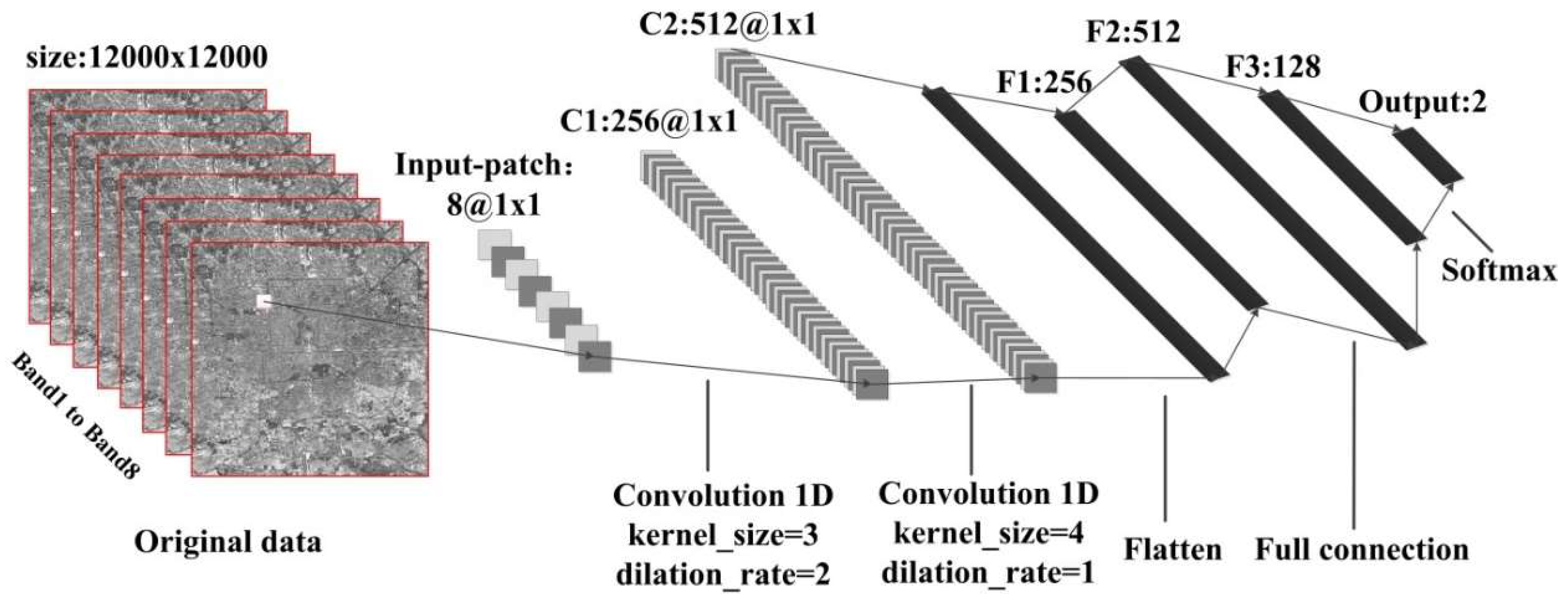
For each pixel, only the spectral information was taken into account without considering the spatial relationship between pixels. Within the convolutional layer, as shown in Figure 5, there were two one-dimensional convolution (Conv1D) layers realizing one-dimensional band directional convolution, which was equivalent to complex band operation. We then used three fully connected layers. To prevent overfitting, one batch-normalization layer and one dropout layer were added. The output layer consisted of a softmax operator, which output two categories. In the whole network, we used the popular function called rectified linear unit (ReLU) to solve the vanishing gradient problem for the training epochs in the network.
3.2.2. CNN_2D Classification
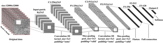
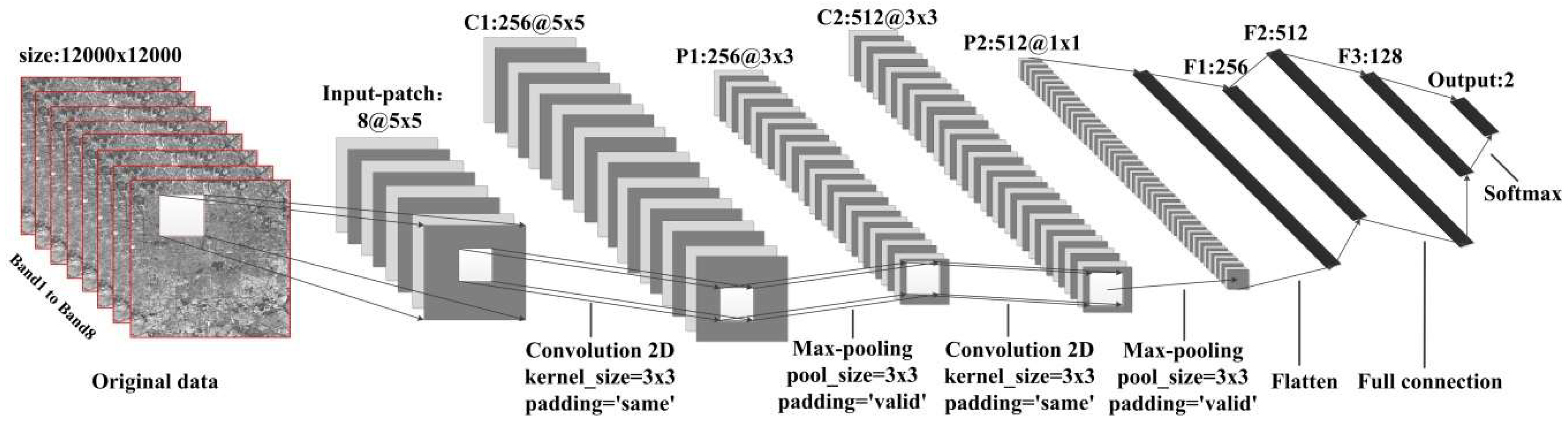
In a 15-m resolution image, the size of a building is generally less than five pixels. For each pixel, the 5-neighborhood was considered, which means that the size of the image patch was 5 × 5 × 8. Therefore, as shown in Figure 6, an image patch with eight bands and a 5 × 5 neighborhood centered on each sample was input into the neural network. Within the convolutional layer, there were two two-dimensional convolution (Conv2D) and two max-pooling layers, which aimed to extract spectral and spatial features, and more high-grade features. In the fully connected layer, we used three fully connected layers. Meanwhile, one batch-normalization layer and one dropout layer were added to prevent overfitting. The output layer consisted of a softmax operator, which outputs two categories. In the whole network, we also used ReLU as the activation function.
4. Experimental Results and Evaluation
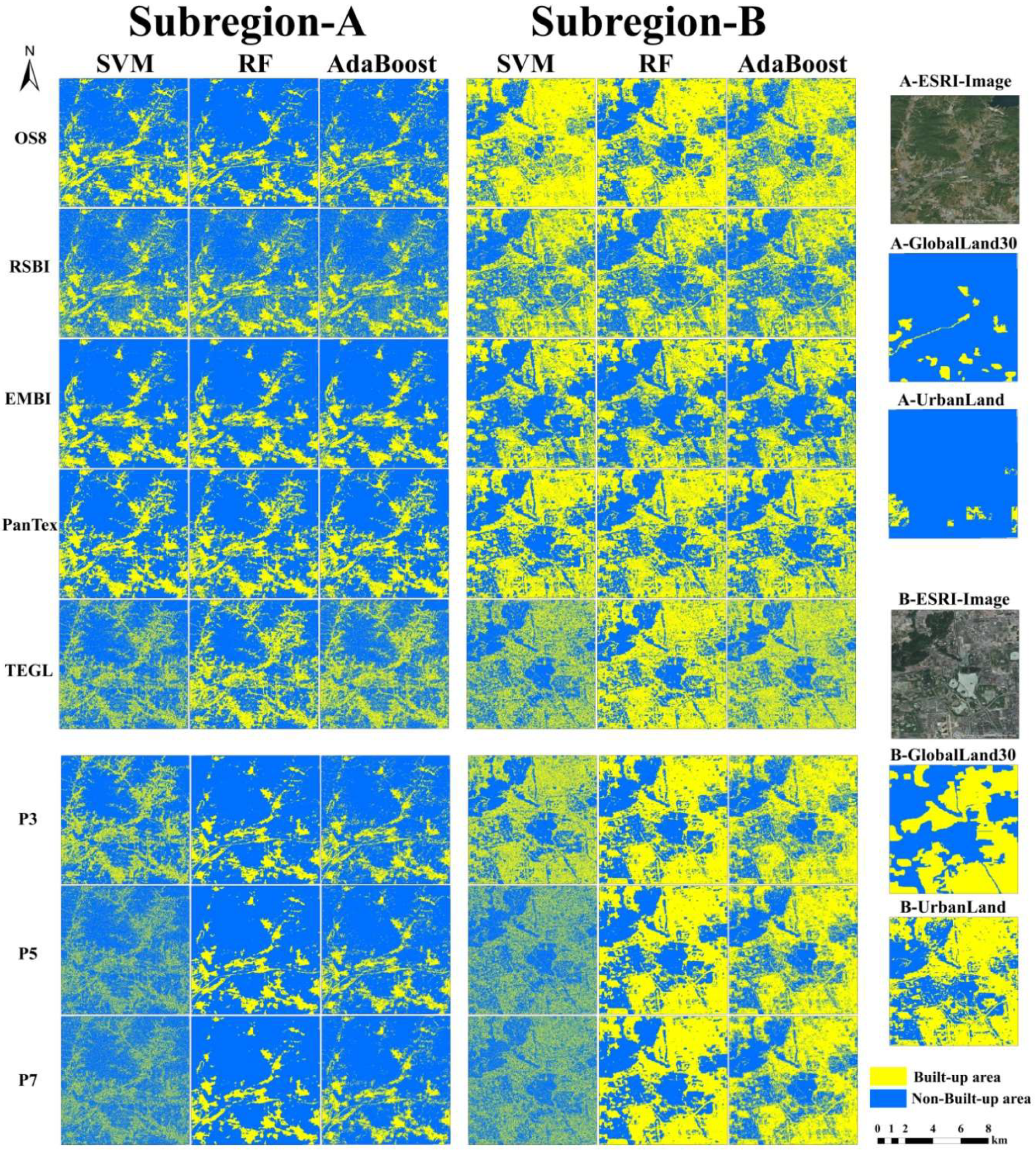
In total, 26 built-up land cover results were produced. However, considering the large range of research, the large amount of map data, and the reduction of the mapping resolution, we cut out the results of two small areas (A and B) for map display. As shown in Figure 7, for feature engineering based on a single pixel, 30 maps were produced using a combination of five features (OS8, RSBI, EMBI, PanTex, and TEGL) and three classifiers (SVM, RF, and AdaBoost). For feature engineering based on image patches, 18 maps were produced using a combination of three kinds of neighborhoods (P3, P5, and P7) and three classifiers (SVM, RF, and AdaBoost). For feature learning, four maps were used, including the result of one-dimensional convolution on a single pixel and the result of two-dimensional convolution on an image patch. The main aim of this paper was to compare the accuracy and efficiency of extracting a 15-m resolution built-up area based on a single pixel and image patch in two cases of feature engineering and feature learning. For completeness, all 52 classified maps for sub-regions A and B were extracted and are provided in Figure 7 and Figure 8. For the sake of qualitative comparison, we compared the results of all the conditions with those of Global-Urban-2015 [56] and GlobalLand30 [52].
A total of 7667 test samples was used for the accuracy evaluation. The test samples were classified to obtain the predictive label of each sample, and then, the confusion matrix shown in Table 4 was obtained according to the real label and the predictive label. The overall accuracy (OA), recall, and precision were calculated based on the confusion matrix: OA represents the correctly predicted sample size for all the samples, recall indicates the size of the predicted built-up sample in all the true built-up samples, and precision indicates the size of the true built-up sample in all the predicted built-up samples. These three precision indices were used to comprehensively evaluate the accuracy of the built-up area extraction.
The OA, Recall, and Precision were calculated using Equations (11)–(13), respectively:
where the meanings of TP, TN, FN, and FP are shown in Table 4.
4.1. Feature Engineering and Feature Learning
From the perspective of feature engineering and feature learning, based on feature engineering classification, the classification results were highly correlated with the setting of features, and the appropriate features were conducive to improving the classification accuracy. However, feature learning does not need to consider manual feature setting. CNN can automatically learn multi-level features from the original image and then achieve classification by black box operation. As shown in Figure 7 and Figure 8 and Table 5 and Table 6, the classification accuracy based on feature learning is generally better than that based on feature engineering. However, in feature engineering, when the original eight bands considered the neighborhood and the classifier was RF, the overall accuracy reached 90%, which is comparable to the results of CNN_2D.
4.2. Single Pixel and Image Patch
Considering a single pixel and image patch, the classification based on a single pixel only considers the feature vectors of the pixel, ignoring the spatial relationship between pixels in the image spatial plane. As shown in Figure 7 and Table 5, overall, the classification effect and accuracy based on the image patch were better than those based on a single pixel; however, the feature dimension of the image patch was large, and there may have been feature redundancy. When training samples are large, a more complex classification model is needed. As shown in Figure 9 and Table 6, CNN based on the image patch had a significant advantage over CNN based on a single pixel.
Under feature engineering, the accuracy of classifications based on a single pixel was significantly lower than that based on an image patch. Comparing OS8, RSBI, EMBI, PanTex, and TEGL, the order of OA and Recall from high to low was as follows: OS8, PanTex, EMBI, RSBI, and TEGL. The original spectrum (OS8) had the best effect, and the OA of OS8 and PanTex was higher than 82%. The analysis shows that the feature dimension is not necessarily related to the improvement of classification accuracy. Highlighting the characteristics of the target category information can help improve classification accuracy. Combining Figure 4 and Figure 7, PanTex and EMBI can effectively distinguish built-up areas, while RSBI and TEGL cannot reflect buildings well. In particular, the five texture features under TEGL have redundancy and conflict. In the five-dimensional feature space, it is difficult to learn the appropriate classification boundary, which leads to a poor classification effect.
As shown in Figure 8 and Figure 10, the built-up area extraction effect based on CNN_2D performed the best. We found many details in the results of CNN_2D that were missing in the other two productions (GlobalLand30 and Global-Urban-2015). One of the reasons for this is that the result of CNN_2D was produced from satellite images with higher spatial resolutions. Consequently, within the urban area, non-built-up areas (e.g., water and vegetation in dense buildings) could be discriminated from built-up areas within the Landsat 8 images. Meanwhile, in the suburbs, small built-up areas and narrow roads could become distinguishable from the background. Another reason is the higher classification accuracy of the CNN.
4.3. Classification Strategy
From the perspective of classification strategy, compared with traditional machine learning algorithms such as SVM, RF, and AdaBoost, CNN has the advantages of autonomous learning, stability, and robustness. Additionally, CNN can learn the dual characteristics of the spectrum and spatial structure in a black box. Users can migrate and use the trained network structure and only need to focus on input and output. As shown in Figure 7 and Figure 8, the classification accuracy of P5-RF and P7-RF differed little from that of CNN_2D and was far superior to the other classification results. CNN has the structure of batch normalization and dropout, which can prevent overfitting. With the increase of the convolutional layer and pooling layer, the network becomes increasingly complex and has stronger fitting and predicting ability. Integrated classifiers (such as RF and AdaBoost), which synthesize the prediction results of all the base classifiers and determine the final category by a voting method, can effectively prevent overfitting and still have higher classification accuracy when the feature dimension is high. However, SVM is more suitable for small sample learning. When the number of samples is too large and the feature dimension is high, most of the training samples are regarded as support vectors, resulting in overfitting, and the final classification accuracy is very low, even worse than a random guess. The OA of P3-SVM, P5-SVM, and P7-SVM were 0.730, 0.525, and 0.525, respectively, and the training accuracy was 1 for all the measures. Overfitting clearly occurred and led to the classification failure.
4.4. Time Complexity
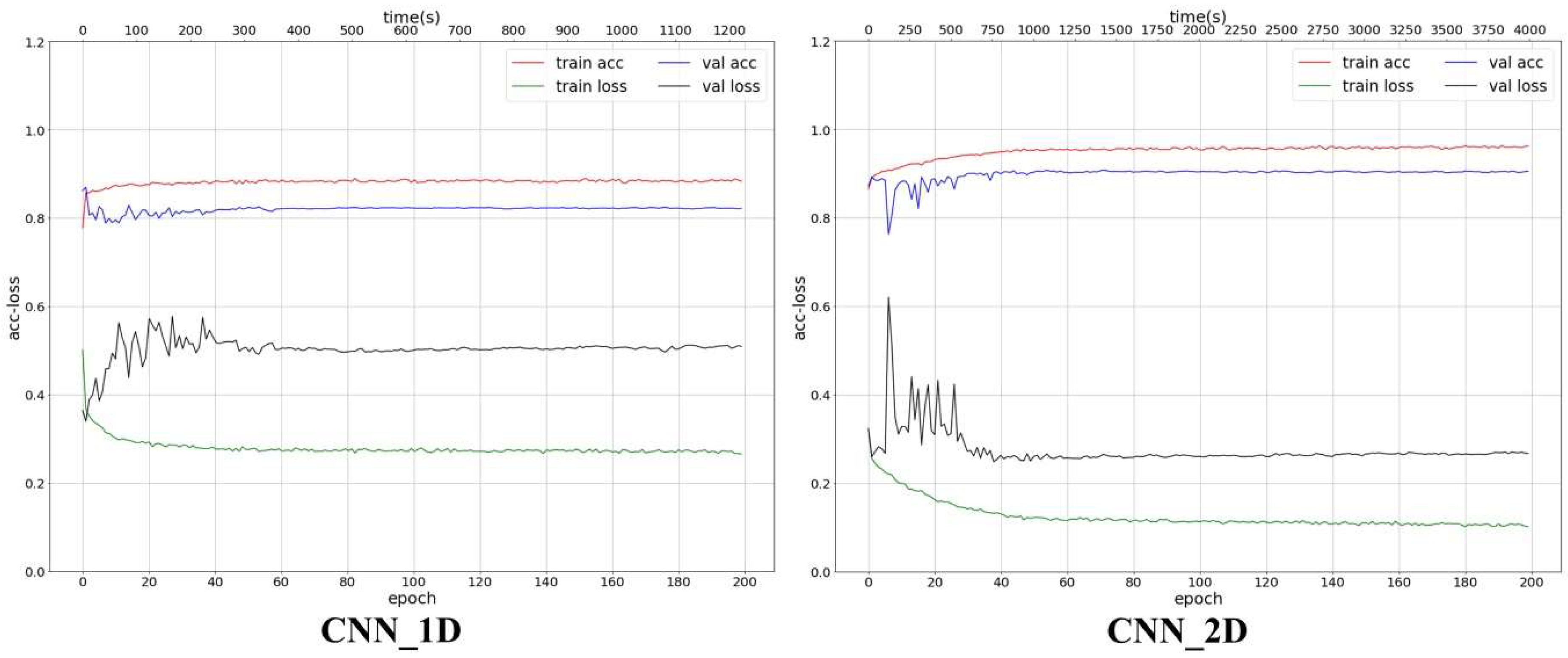
According to the training time of the model, the time of the classifiers based on feature engineering was significantly less than that of the models based on feature learning. As shown in Table 7 and Figure 11, the training time of the classifiers based on feature engineering was less than 300 s, while that of the models based on feature learning was more than 400 s. For feature engineering, the training time of the classifiers based on image patch (P3, P5, and P7) was significantly higher than that of the classifiers based on single pixel. The lower the dimension of the feature, the shorter the training time. Compared with the three classifiers, SVM, RF, and AdaBoost, the training time of SVM was significantly longer than that of RF and AdaBoost. When the feature dimension was very low (below three), the training time of RF and AdaBoost was extremely short. For feature learning, when the model was stable, the training time of CNN_1D and CNN_2D models was 400 s and 1000 s, respectively, so the time complexity of CNN_2D was higher than that of CNN_1D.
5. Discussion
5.1. Support Vectors of SVM
As shown in Figure 7 and Figure 9 and Table 5 and Table 8, P3-SVM, P5-SVM, and P7-SVM were overfitted, and the number of support vectors in the 11,499 training samples was 11,431, 11,485, and 11,493, respectively. Therefore, all the training samples were regarded as support vectors, so the model training was too complex with poor generalization ability and was unable to accurately predict the unclassified data. In the above experimental analysis, the penalty coefficient (C) and Gamma, which are the key parameters, were set to 10 and 100, respectively. The setting of these two parameters was reasonable and scientifically based on prior knowledge and experimental attempts. When the features were OS8, RSBI, EMBI, PanTex, and TEGL, the classification results met expectations, and no overfitting was observed. When considering 3, 5, and 7 neighborhoods, the number of features was 72, 200, and 392, respectively, the feature dimension increased significantly, and these high-dimensional features had greater correlation and redundancy, resulting in overfitting in SVM.
We analyzed the principle of the SVM classification algorithm. The overfitting was mainly due to the irregular distribution and clustering of the training data in the feature space, resulting in a large number of samples as support vectors, and the classification boundary was very complex. Therefore, we utilized the L2 regularization method provided by Python sklearn to process the original eight-band data and eliminate the noise and scattering of the data and then used SVM to classify. The results show that the overfitting was effectively suppressed. As shown in Table 8 and Table 9, after L2 regularization, the number of support vectors corresponding to OS8, P3, P5, and P7 was significantly reduced, and the OAs were 0.800, 0.832, 0.858, and 0.874, respectively. The classification effect significantly improved, which agreed with logic and expectations.
5.2. CNN_2D versus VGG16
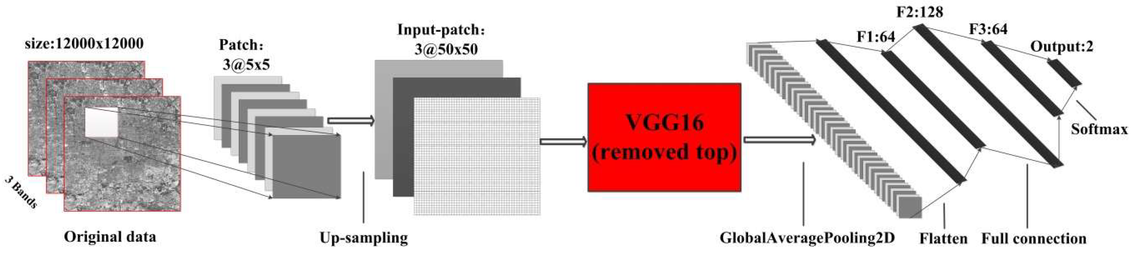
We compared the results of CNN_2D with VGG16 [40]. As shown in Figure 12, we reserved the weight of the convolution layers and the pooling layers of VGG16 and reset the top layers, including the fully-connected layers, the BatchNormalization layer and the softmax layer. Because the original image has 8 bands and cannot be directly input to VGG16, we fused panchromatic and multi-spectral bands by Gram–Schmidt pan sharpening to obtain the fusion image with 15-m resolution and seven bands. Then, we considered three bands in two ways: (1) The first three principal components were taken after principal component analysis; and (2) the 432 bands representing red, green and blue (RGB) were taken directly. For VGG16, there had to be three channels of input data, and the size had to be greater than 48 × 48, which were determined by the parameters of the VVG16 model in python–keras, so the neighborhood of 5 × 5 was up-sampled to 50 × 50 by nearest neighbor sampling.
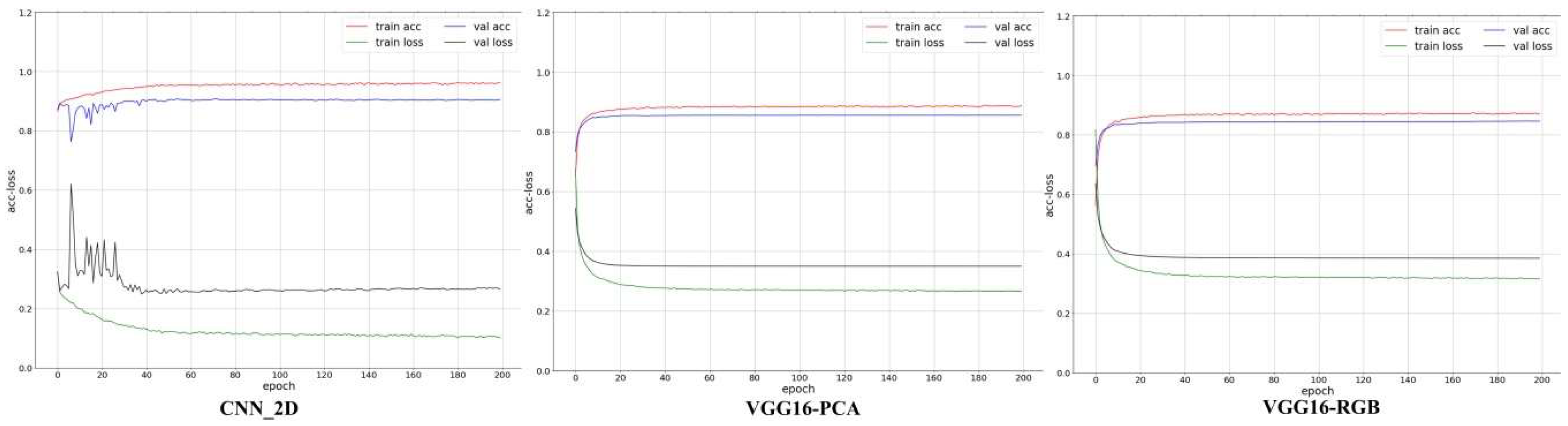
We set the ratio of the training samples and validation samples to 6:4 for training the proposed CNN and VGG16. The accuracy and loss of the training process are shown in Figure 13.
We recorded the training accuracy, training loss, test accuracy, test loss, and training time of 200 epochs. Table 10 shows that the accuracy of the CNN_2D was significantly better than that of VGG16, and the training time was greatly shortened. In Figure 14, the classification effect of CNN_2D was obviously greater than that of VGG16, and the extraction of built-up areas was more detailed and accurate.
6. Conclusions
This paper presented a unique investigation to provide a full evaluation of OLI imagery for 15-m resolution built-up area classification from two viewpoints. First, traditional feature engineering and modern feature learning strategies were compared. Next, the influence of a single pixel and image patch was examined. In contrast, previous studies have generally tended to conduct limited comparisons between, for instance, coarse and fine resolution or pixel- and object-based classification. First, our training samples were automatically selected and filtered based on the existing product data. Then, we made a multi-level and all-around comparison from two different perspectives: (1) single pixel and image patch; and (2) feature engineering and feature learning. In feature engineering, we took into account the spectrum, morphology, texture, and other characteristics. In previous studies, there has been no such detailed and comprehensive consideration. Finally, our work was conducted on a relatively large image area—the city of Beijing, China, and its surroundings—ensuring that urban land cover information is generated at a scale of practical value. In contrast, earlier experiments have often been limited to very small, local areas. All the tests were evaluated by the same set of test samples with overall accuracy and a Kappa coefficient. The results can be summarized as follows:
- (1)
- The classification accuracy based on feature learning is generally better than that based on feature engineering. However in feature engineering, when the original eight bands consider the neighborhood and the classifier is RF, the overall accuracy reaches 90%, which is comparable to the results of CNN_2D.
- (2)
- The classification effect and accuracy based on the image patch are better than those based on a single pixel; however, the feature dimension of the image patch is large, and there may be feature redundancy. When training samples are large, a more complex classification model is needed. CNNs based on image patches have a significant advantage over CNNs based on single pixels. The results of CNN_2D, water, and vegetation in dense buildings can be discriminated from built-up areas within the Landsat 8 images. Meanwhile, in the suburbs, small built-up areas and narrow roads become distinguishable from the background.
- (3)
- Compared with traditional machine learning algorithms, such as SVM, RF, and AdaBoost, CNN has the advantages of autonomous learning, stability, and robustness. The classification accuracy of P5-RF and P7-RF differs little from that of CNN_2D and is far superior to the other classification results. The accuracy of CNN_2D is significantly better than that of VGG16. L2 regularization can eliminate the noise and scattering of the original eight-band data, effectively suppress SVM overfitting, and significantly reduce the number of support vectors.
The results of this paper can be used as a reference for the extraction and mapping of large 15-m resolution building areas. The comprehensive comparison of classification algorithms can help researchers in remote sensing image pattern recognition to understand the principle and applicability of the algorithm and better carry out scientific research. In this paper, a large number of samples were selected automatically based on existing data products, which is of great significance for improving the efficiency and effectiveness of supervised classification and can save considerable manpower and time. At the same time, there are some shortcomings to this research, such as not using multi-scale remote sensing data (low-, medium-, and high-resolution) for the comparative analysis of built-up area extraction, the fact that the spatial relationship of the pixels in an image patch was not analyzed in depth, and the fact that the hidden layer of CNN was not displayed and analyzed in detail. We will study these problems in follow-up work and hope that more scholars will develop an interest and become involved.
Author Contributions
Conceptualization, H.T.; Funding acquisition, H.T.; Investigation, H.T. and T.Z.; Methodology, T.Z.; Software, T.Z.; and Supervision, H.T.
Funding
This work was supported by the National Key R&D Program of China (No. 2017YFB0504104) and the National Natural Science Foundation of China (No. 41571334).
Conflicts of Interest
The authors declare no conflict of interest.
References
- Chen, X.H.; Cao, X.; Liao, A.P.; Chen, L.J.; Peng, S.; Lu, M.; Chen, J.; Zhang, W.W.; Han, G.; Wu, H.; et al. Global mapping of artificial surfaces at 30-m resolution. Sci. China Earth Sci. 2016, 59, 2295–2306. [Google Scholar] [CrossRef]
- Chaudhuri, D.; Kushwaha, N.K.; Samal, A.; Agarwal, R.C. Automatic Building Detection from High-Resolution Satellite Images Based on Morphology and Internal Gray Variance. IEEE J. Sel. Top. Appl. Earth Obs. Remote Sens. 2016, 9, 1767–1779. [Google Scholar] [CrossRef]
- Jin, X.; Davis, C.H. Automated building extraction from high-resolution satellite imagery in urban areas using structural, contextual, and spectral information. EURASIP J. Adv. Signal Process. 2005, 2005, 2196–2206. [Google Scholar] [CrossRef]
- Pesaresi, M.; Guo, H.; Blaes, X.; Ehrlich, D.; Ferri, S.; Gueguen, L.; Halkia, M.; Kauffmann, M.; Kemper, T.; Lu, L.L.; et al. A Global Human Settlement Layer from Optical HR/VHR RS Data: Concept and First Results. IEEE J. Sel. Top. Appl. Earth Obs. Remote Sens. 2013, 6, 2102–2131. [Google Scholar] [CrossRef]
- Goldblatt, R.; Stuhlmacher, M.F.; Tellman, B.; Clinton, N.; Hanson, G.; Georgescu, M.; Wang, C.Y.; Serrano-Candela, F.; Khandelwa, A.K.; Cheng, W.H.; et al. Using Landsat and nighttime lights for supervised pixel-based image classification of urban land cover. Remote Sens. Environ. 2018, 205, 253–275. [Google Scholar] [CrossRef]
- Yang, J.; Meng, Q.Y.; Huang, Q.Q.; Sun, Z.H. A New Method of Building Extraction from High Resolution Remote Sensing Images Based on NSCT and PCNN. Int. Conf. Agro-Geoinform. 2016, 428–432. [Google Scholar]
- Zhong, P.; Wang, R. A Multiple Conditional Random Fields Ensemble Model for Urban Area Detection in Remote Sensing Optical Images. IEEE Trans. Geosci. Remote Sens. 2007, 45, 3978–3988. [Google Scholar] [CrossRef]
- Schaaf, C.B.; Gao, F.; Strahler, A.H.; Lucht, W.; Tsang, T.; Strugnell, N.C.; Zhang, X.Y.; Jin, Y.F.; Muller, J.P.; Lewis, P.; et al. First operational BRDF, albedo nadir reflectance products from MODIS. Remote Sens. Environ. 2002, 83, 135–148. [Google Scholar] [CrossRef] [Green Version]
- Zhu, X.X.; Tuia, D.; Mou, L.C.; Xia, G.S.; Zhang, L.P.; Xu, F.; Fraundorfer, F. Deep Learning in Remote Sensing: A Comprehensive Review and List of Resources. IEEE Geosci. Remote Sens. Mag. 2017, 5, 8–36. [Google Scholar] [CrossRef] [Green Version]
- Minar, M.R.; Naher, J. Recent Advances in Deep Learning: An Overview. arXiv, 2018; arXiv:1807.08169. [Google Scholar]
- Alom, M.Z.; Taha, T.M.; Yakopcic, C.; Westberg, S.; Hasan, M.; Van Esesn, B.; Awwal, A.S.; Asari, V.K. The History Began from AlexNet: A Comprehensive Survey on Deep Learning Approaches. arXiv, 2018; arXiv:1803.01164. [Google Scholar]
- Li, C.; Wang, J.; Wang, L.; Hu, L.Y.; Gong, P. Comparison of Classification Algorithms and Training Sample Sizes in Urban Land Classification with Landsat Thematic Mapper Imagery. Remote Sens. 2014, 6, 964–983. [Google Scholar] [CrossRef] [Green Version]
- Momeni, R.; Aplin, P.; Boyd, D.S. Mapping Complex Urban Land Cover from Spaceborne Imagery: The Influence of Spatial Resolution, Spectral Band Set and Classification Approach. Remote Sens. 2016, 8, 88. [Google Scholar] [CrossRef]
- Lu, D.; Weng, Q. A survey of image classification methods and techniques for improving classification performance. Int. J. Remote Sens. 2007, 28, 823–870. [Google Scholar] [CrossRef] [Green Version]
- Xiang, D.; Tang, T.; Canbin, H.; Fan, Q.H.; Su, Y. Built-up Area Extraction from PolSAR Imagery with Model-Based Decomposition and Polarimetric Coherence. Remote Sens. 2016, 8, 685. [Google Scholar] [CrossRef]
- Xiang, D.; Tang, T.; Ban, Y.; Su, Y.; Kuang, G. Unsupervised polarimetric SAR urban area classification based on model-based decomposition with cross scattering. ISPRS J. Photogramm. Remote Sens. 2016, 116, 86–100. [Google Scholar] [CrossRef]
- Xiang, D.; Tang, T.; Ban, Y.; Su, Y.; Samhällsplanering, Q.M.; Skolan, F.A.O.; Samhällsbyggnad; Geoinformatik. Man-Made Target Detection from Polarimetric SAR Data via Nonstationarity and Asymmetry. IEEE J. Sel. Top. Appl. Earth Obs. Remote Sens. 2016, 9, 1459–1469. [Google Scholar] [CrossRef]
- Zha, Y.; Gao, J.; Ni, S. Use of normalized difference built-up index in automatically mapping urban areas from TM imagery. Int. J. Remote Sens. 2003, 24, 583–594. [Google Scholar] [CrossRef]
- Xu, H. A new index for delineating built-up land features in satellite imagery. Int. J. Remote Sens. 2008, 29, 4269–4276. [Google Scholar] [CrossRef]
- Pesaresi, M.; Gerhardinger, A.; Kayitakire, F. A Robust Built-Up Area Presence Index by ani-sotropic Rotation-Invariant Texture Measure. IEEE J. Sel. Top. Appl. Earth Obs. Remote Sens. 2009, 1, 180–192. [Google Scholar] [CrossRef]
- Benedek, C.; Descombes, X.; Zerubia, J. Building development monitoring in multitemporal remotely sensed image pairs with stochastic birth-death dynamics. IEEE Trans. Pattern Anal. Mach. Intell. 2012, 34, 33–50. [Google Scholar] [CrossRef] [PubMed]
- Grinias, I.; Panagiotakis, C.; Tziritas, G. MRF-based Segmentation and Unsupervised Classification for Building and Road Detection in Peri-urban Areas of High-resolution. ISPRS J. Photogramm. Remote Sens. 2016, 122, 145–166. [Google Scholar] [CrossRef]
- Inglada, J. Automatic recognition of man-made objects in high resolution optical remote sensing images by SVM classification of geometric image features. ISPRS J. Photogramm. Remote Sens. 2007, 62, 236–248. [Google Scholar] [CrossRef]
- Anagiotakis, C.; Kokinou, E.; Sarris, A. Curvilinear Structure Enhancement and Detection in Geophysical Images. IEEE Trans. Geosci. Remote Sens. 2011, 49, 2040–2048. [Google Scholar] [CrossRef]
- Lowe, D.G. Distinctive image features from scale-invariant keypoints. Int. J. Comput. Vis. 2004, 60, 91–110. [Google Scholar] [CrossRef]
- LeCun, Y.; Bengio, Y.; Hinton, G. Deep learning. Nature 2015, 521, 436–444. [Google Scholar] [CrossRef] [PubMed]
- Schmidhuber, J. Deep learning in neural networks: An overview. Neural Netw. 2015, 61, 85–117. [Google Scholar] [CrossRef] [Green Version]
- Silver, D.; Schrittwieser, K.; Antonoglou, L.; Huang, A.; Hubert, T.; Baker, L.; Lai, M.; Bolton, A.; Chen, Y.T.; Lillicrap, T.; et al. Mastering the game of Go without human knowledge. Nature 2017, 550, 354–359. [Google Scholar] [CrossRef] [PubMed]
- Li, Y. Deep Reinforcement Learning: An Overview. arXiv, 2017; arXiv:1701.07274. [Google Scholar]
- Andreas, J.; Klein, D.; Levine, S. Modular Multitask Reinforcement Learning with Policy Sketches. arXiv, 2016; arXiv:1611.01796. [Google Scholar]
- Anschel, O.; Baram, N.; Shimkin, N. Averaged-DQN: Variance Reduction and Stabilization for Deep Reinforcement Learning. arXiv, 2016; arXiv:1611.01929. [Google Scholar]
- Arulkumaran, K.; Deisenroth, K.; Deisenroth, M.; Bharath, A.A. A Brief Survey of Deep Reinforcement Learning. arXiv, 2017; arXiv:1708.05866. [Google Scholar] [CrossRef]
- Babaeizadeh, M.; Frosio, L.; Tyree, S.; Clemons, J.; Kautz, J. Reinforcement Learning through Asynchronous Advantage Actor-Critic on a GPU. arXiv, 2016; arXiv:1611.06256. [Google Scholar]
- Hinton, G.E.; Salakhutdinov, R.R. Reducing the dimensionality of data with neural networks. Science 2006, 313, 504–507. [Google Scholar] [CrossRef] [PubMed]
- Ackley, D.H.; Hinton, G.E.; Sejnowski, T.J. A Learning Algorithm for Boltzmann Machines. Connectionist Models and Their Implications: Readings from Cognitive Science; Ablex Publishing Corp.: New York, NY, USA, 1988; pp. 147–169. [Google Scholar]
- Creswell, A.; White, T.; Dumoulin, V.; Arulkumaran, K.; Sengupta, B.; Bharath, A. Generative Adversarial Networks: An Overview. IEEE Signal Process. Mag. 2017, 35, 53–65. [Google Scholar] [CrossRef]
- Zhao, W.; Du, S. Learning multiscale and deep representations for classifying remotely sensed imagery. ISPRS J. Photogramm. Remote Sens. 2016, 113, 155–165. [Google Scholar] [CrossRef]
- Han, J.; Zhang, D.; Cheng, G.; Guo, L.; Ren, J.C. Object Detection in Optical Remote Sensing Images Based on Weakly Supervised Learning and High-Level Feature Learning. IEEE Trans. Geosci. Remote Sens. 2015, 53, 3325–3337. [Google Scholar] [CrossRef] [Green Version]
- Krizhevsky, A.; Sutskever, I.; Hinton, G.E. ImageNet classification with deep convolutional neural networks. In International Conference on Neural Information Processing Systems; Curran Associates Inc.: Red Hook, NY, USA, 2012; pp. 1097–1105. [Google Scholar]
- Simonyan, K.; Zisserman, A. Very Deep Convolutional Networks for Large-Scale Image Recognition. arXiv, 2014; arXiv:1409.1556. [Google Scholar]
- Szegedy, C.; Liu, W.; Jia, Y.; Sermanet, P.; Reed, S.; Anguelov, D.; Erhan, D.; Vanhoucke, V.; Rabinovich, A. Going Deeper with Convolutions. In Proceedings of the 2015 IEEE Conference on Computer Vision and Pattern Recognition (CVPR), Boston, MA, USA, 7–12 June 2015; pp. 1–9. [Google Scholar]
- He, K.; Zhang, X.; Ren, S.; Sun, J. Deep Residual Learning for Image Recognition. In Proceedings of the 2016 IEEE Conference on Computer Vision and Pattern Recognition (CVPR), Las Vegas, NV, USA, 27–30 June 2016; pp. 770–778. [Google Scholar]
- Castelluccio, M.; Poggi, G.; Sansone, C.; Verdoliva, L. Land Use Classification in Remote Sensing Images by Convolutional Neural Networks. Acta Ecol. Sin. 2015, 28, 627–635. [Google Scholar]
- Vakalopoulou, M.; Karantzalos, K.; Komodakis, N.; Paragios, N. Building detection in very high resolution multispectral data with deep learning features. In Proceedings of the 2015 IEEE International Geoscience and Remote Sensing Symposium (IGARSS), Milan, Italy, 26–31 July 2015; pp. 1873–1876. [Google Scholar]
- Huang, Z.; Cheng, G.; Wang, H.; Li, H.; Shi, L.; Pan, C. Building extraction from multi-source remote sensing images via deep deconvolution neural networks. In Proceedings of the 2016 IEEE International Geoscience and Remote Sensing Symposium (IGARSS), Beijing, China, 10–15 July 2016; pp. 1835–1838. [Google Scholar]
- Makantasis, K.; Karantzalos, K.; Doulamis, A.; Loupos, K. Deep Learning-Based Man-Made Object Detection from Hyperspectral Data. Lect. Notes Comput. Sci. 2015, 717–727. [Google Scholar]
- Yang, N.; Tang, H.; Sun, H.; Yang, X. DropBand: A Simple and Effective Method for Promoting the Scene Classification Accuracy of Convolutional Neural Networks for VHR Remote Sensing Imagery. IEEE Geosci. Remote Sens. Lett. 2018, 5, 257–261. [Google Scholar] [CrossRef]
- Wang, L.; Zhu, J.H.; Xu, Y.Q.; Wang, Z.Q. Urban Built-Up Area Boundary Extraction and Spatial-Temporal Characteristics Based on Land Surface Temperature Retrieval. Remote Sens. 2018, 10, 473. [Google Scholar] [CrossRef]
- Ning, X.; Lin, X. An Index Based on Joint Density of Corners and Line Segments for Built-Up Area Detection from High Resolution Satellite Imagery. ISPRS Int. J. Geo-Inf. 2017, 6, 338. [Google Scholar] [CrossRef]
- Friedl, M.A.; Mciver, D.K.; Hodges, J.C.F.; Zhang, X.Y.; Muchoney, D.; Strahler, A.H.; Woodcock, C.E.; Gopal, S.; Schneider, A.; Cooper, A.; et al. Global land cover mapping from MODIS: Algorithms and early results. Remote Sens. Environ. 2002, 83, 287–302. [Google Scholar] [CrossRef]
- Gong, P.; Wang, J.; Yu, L.; Zhao, Y.C.; Zhao, Y.Y.; Liang, L.; Niu, Z.G.; Huang, X.M.; Fu, H.H.; Liu, S.; et al. Finer resolution observation and monitoring of global land cover: First mapping results with Landsat TM and ETM+ data. Int. J. Remote Sens. 2013, 34, 2607–2654. [Google Scholar] [CrossRef]
- Chen, J.; Chen, J.; Liao, A.; Cao, X.; Chen, L.J.; Chen, X.H.; He, C.Y.; Han, G.; Peng, S.; Lu, M.; et al. Global land cover mapping at 30 m resolution: A POK-based operational approach. ISPRS J. Photogramm. Remote Sens. 2015, 103, 7–27. [Google Scholar] [CrossRef]
- Pesaresi, M.; Ehrlich, D.; Ferri, S.; Florczyk, A.; Carneiro Freire, S.; Halkia, S.; Julea, A.; Kemper, T.; Soille, P.; Syrris, V. Operating Procedure for the Production of the Global Human Settlement Layer from Landsat Data of the Epochs 1975, 1990, 2000, and 2014; EUR 27741; Publications Office of the European Union: Luxembourg, 2016; JRC97705. [Google Scholar]
- Gorelick, N.; Hancher, M.; Dixon, M.; Ilyushchenko, S.; Thau, D.; Moore, R. Google Earth Engine: Planetary-scale geospatial analysis for everyone. Remote Sens. Environ. 2017, 202, 18–27. [Google Scholar] [CrossRef]
- Liu, X.; Hu, G.; Ai, B.; Li, X.; Shi, Q. A Normalized Urban Areas Composite Index (NUACI) Based on Combination of DMSP-OLS and MODIS for Mapping Impervious Surface Area. Remote Sens. 2015, 7, 17168–17189. [Google Scholar] [CrossRef] [Green Version]
- Liu, X.; Hu, G.; Chen, Y.; Li, X.; Xu, X.C.; Li, S.Y.; Pei, F.S.; Wang, S.J. High-resolution multi-temporal mapping of global urban land using Landsat images based on the Google Earth Engine Platform. Remote Sens. Environ. 2018, 209, 227–239. [Google Scholar] [CrossRef]
- Zhang, P.; Sun, Q.; Liu, M.; Li, J.; Sun, D.F. A Strategy of Rapid Extraction of Built-Up Area Using Multi-Seasonal Landsat-8 Thermal Infrared Band 10 Images. Remote Sens. 2017, 9, 1126. [Google Scholar] [CrossRef]
- Ma, X.; Tong, X.; Liu, S.; Luo, X.; Xie, H.; Li, C.M. Optimized Sample Selection in SVM Classification by Combining with DMSP-OLS, Landsat NDVI and GlobeLand30 Products for Extracting Urban Built-Up Areas. Remote Sens. 2017, 9, 236. [Google Scholar] [CrossRef]
- Goldblatt, R.; You, W.; Hanson, G.; Khandelwal, A.K. Detecting the Boundaries of Urban Areas in India: A Dataset for Pixel-Based Image Classification in Google Earth Engine. Remote Sens. 2016, 8, 634. [Google Scholar] [CrossRef]
- Huang, X.; Zhang, L. A Multidirectional and Multiscale Morphological Index for Automatic Building Extraction from Multispectral GeoEye-1 Imagery. Photogramm. Eng. Remote Sens. 2011, 77, 721–732. [Google Scholar] [CrossRef]
- Smith, J.R.; Chang, S. Automated Binary Texture Feature Sets for Image Retrieval. Acoust. Speech Signal Process. Conf. IEEE Int. Conf. IEEE Comput. Soc. 1996, 4, 2239–2242. [Google Scholar]
- Haralick, R.M.; Shanmugam, K.; Dinstein, I.H. Textural features for image classification. IEEE Trans. Syst. Man Cybern. 1973, 6, 610–621. [Google Scholar] [CrossRef]
- Haralick, R.M. Statistical and structural approaches to texture. Proc. IEEE 1979, 67, 786–804. [Google Scholar] [CrossRef]
- Tamura, H.; Mori, S.; Yamawaki, T. Textural features corresponding to visual perception. IEEE Trans. Syst. Man Cybern. 1978, 8, 460–473. [Google Scholar] [CrossRef]
- Pelletier, C.; Valero, S.; Inglada, J.; Champion, N.; Dedieu, G. Assessing the robustness of Random Forests to map land cover with high resolution satellite image time series over large areas. Remote Sens. Environ. 2016, 187, 156–168. [Google Scholar] [CrossRef]
Figure 1.
Research area and samples (Subregion B is an urban central region with dense buildings, while subregion A is a suburban region with sparse buildings).
Figure 1.
Research area and samples (Subregion B is an urban central region with dense buildings, while subregion A is a suburban region with sparse buildings).

Figure 2.
Sample generation and correction. ESA: European Space Agency; OSM: OpenStreetMap.

Figure 3.
Feature maps of different feature descriptors. ASM: angular second moment; CON: contrast; COR: correlation; ENT: entropy; and HOM: homogeneity (A and B represent the two subregions).
Figure 3.
Feature maps of different feature descriptors. ASM: angular second moment; CON: contrast; COR: correlation; ENT: entropy; and HOM: homogeneity (A and B represent the two subregions).

Figure 4.
The 12 displacement vectors in the 5 × 5 window.

Figure 5.
Network structure of CNN_1D.

Figure 6.
Network structure of CNN_2D.

Figure 7.
Classification results based on feature engineering. (The first five rows are the classification results of three classifiers within five set features. The last three rows are the classification results of three classifiers within three kinds of image patch.)
Figure 7.
Classification results based on feature engineering. (The first five rows are the classification results of three classifiers within five set features. The last three rows are the classification results of three classifiers within three kinds of image patch.)

Figure 8.
Classification results based on feature learning (A and B represent the two subregions. The first column is the online images of ERSI. The second and third columns represent the classification results of CNN_1D and CNN_2D, respectively. The fourth and fifth columns represent the results of GlobalLand30 and UrbanLand, respectively).

Figure 9.
Classification accuracies of the built-up area based on feature engineering.

Figure 10.
Classification accuracies of the built-up area based on feature learning.

Figure 11.
The training process of the CNN_1D and CNN_2D (training time: s).

Figure 12.
Transfer learning and fine-tuning of VGG16.

Figure 13.
Accuracy and loss in the training process of the proposed CNN_2D, VGG16-PCA, and VGG16-RGB.
Figure 13.
Accuracy and loss in the training process of the proposed CNN_2D, VGG16-PCA, and VGG16-RGB.

Figure 14.
Results of built-up area by CNN_2D, VGG16-PCA, and VGG16-RGB (A and B represent the two subregions. The first column is the online images of ERSI. The second column represents the classification results of CNN_2D. The third and fourth columns represent the classification results of VGG16-PCA and VGG16-RGB, respectively).


Table 1.
Comparison of Landsat 7 and Landsat 8 satellite bands.
| Landsat 8-OLI | Landsat 7-ETM+ | ||||||
|---|---|---|---|---|---|---|---|
| Band Index | Band Name | Bandwidth (μm) | Resolution (m) | Band Index | Band Name | Bandwidth (μm) | Resolution (m) |
| Band 1 | COASTAL | 0.43–0.45 | 30 | ||||
| Band 2 | BLUE | 0.45–0.51 | 30 | Band 1 | BLUE | 0.45–0.52 | 30 |
| Band 3 | GREEN | 0.53–0.59 | 30 | Band 2 | GREEN | 0.52–0.60 | 30 |
| Band 4 | RED | 0.64–0.67 | 30 | Band 3 | RED | 0.63–0.69 | 30 |
| Band 5 | NIR | 0.85–0.88 | 30 | Band 4 | NIR | 0.77–0.90 | 30 |
| Band 6 | SWIR1 | 1.57–1.65 | 30 | Band 5 | SWIR1 | 1.55–1.75 | 30 |
| Band 7 | SWIR2 | 2.11–2.29 | 30 | Band 7 | SWIR2 | 2.09–2.35 | 30 |
| Band 8 | PAN | 0.50–0.68 | 15 | Band 8 | PAN | 0.52–0.90 | 15 |
Table 2.
Overall framework of method and technology.
| Feature Engineering | Feature Learning | |||||
|---|---|---|---|---|---|---|
| Feature Description | Abbreviations | Classifier | Network Architecture | Abbreviations | ||
| Pixel | Spectrum | Original eight Bands | OS8 | CNN with one-dimensional convolution on inputting bands of each pixel | CNN_1D | |
| Pan + NDBI + IBI | RSBI | |||||
| Morphology | Pan + EMBI | EMBI | SVM | |||
| Texture | Pan + Built-up presence index | PanTex | RF | |||
| Texture from GLCM | TEGL | |||||
| Patch | Original eight Bands | 3 × 3 neighborhood | P3 | AdaBoost | CNN fed with an image patch of size 5 × 5 | CNN_2D |
| 5 × 5 neighborhood | P5 | |||||
| 7 × 7 neighborhood | P7 | |||||
Table 3.
Parameters of the classifiers used in our experiments (Python sklearn).
| Algorithm | Abbreviation | Parameter Type | Parameter Name (sklearn) | Parameter Set |
|---|---|---|---|---|
| Support Vector Machine | SVM | kernel-type | kernel | rbf |
| penalty coefficient | C | 10 | ||
| gamma | gamma | 100 | ||
| Random Forests | RF | base classifier | base_estimator | decision Tree |
| number of trees | n_estimators | 60 | ||
| AdaBoost Classifier | AdaBoost | base classifier | base_estimator | decision Tree |
| number of trees | n_estimators | 60 | ||
| learning rate | learning_rate | 10−3 |
Table 4.
The representation of the confusion matrix for the test samples.
| Prediction | ||||
|---|---|---|---|---|
| Non-Built-Up | Built-Up | Sum | ||
| Ground Truth | Non-Built-up | True Negative (TN) | False Positive (FP) | Actual Negative (TN + FP) |
| Built-up | False Negative (FN) | True Positive (TP) | Actual Positive (FN + TP) | |
| Sum | Predicted Negative (TN + FN) | Predicted Positive (FP + TP) | TN+ TP+ FN+ FP | |
Table 5.
Accuracy evaluation based on feature engineering.
| Feature Engineering | SVM | RF | AdaBoost | ||||||
|---|---|---|---|---|---|---|---|---|---|
| OA | Recall | Precision | OA | Recall | Precision | OA | Recall | Precision | |
| OS8 | 0.849 | 0.922 | 0.794 | 0.887 | 0.904 | 0.864 | 0.841 | 0.834 | 0.831 |
| RSBI | 0.782 | 0.762 | 0.774 | 0.805 | 0.781 | 0.802 | 0.780 | 0.745 | 0.781 |
| EMBI | 0.810 | 0.760 | 0.825 | 0.810 | 0.760 | 0.825 | 0.809 | 0.755 | 0.827 |
| PanTex | 0.824 | 0.825 | 0.808 | 0.821 | 0.820 | 0.805 | 0.817 | 0.811 | 0.804 |
| TEGL | 0.662 | 0.517 | 0.693 | 0.758 | 0.733 | 0.752 | 0.696 | 0.664 | 0.686 |
| P3 | 0.730 | 0.960 | 0.644 | 0.900 | 0.902 | 0.889 | 0.850 | 0.838 | 0.841 |
| P5 | 0.525 | 0.001 | 0.429 | 0.903 | 0.906 | 0.891 | 0.855 | 0.839 | 0.853 |
| P7 | 0.525 | 0.000 | 0.000 | 0.906 | 0.907 | 0.896 | 0.855 | 0.846 | 0.848 |
Table 6.
Accuracy evaluation based on feature learning.
| CNN Model | Training Accuracy | OA | Recall | Precision |
|---|---|---|---|---|
| CNN_1D | 0.872 | 0.823 | 0.675 | 0.935 |
| CNN_2D | 0.968 | 0.901 | 0.915 | 0.882 |
Table 7.
The training time of the different classifier based on feature learning (unit: s).
| Features | SVM | RF | AdaBoost |
|---|---|---|---|
| OS8 | 32.86 | 0.44 | 0.03 |
| RSBI | 24.39 | 0.35 | 1.07 |
| EMBI | 3.87 | 0.21 | 0.44 |
| PanTex | 3.16 | 0.2 | 0.44 |
| TEGL | 32.78 | 0.56 | 1.93 |
| P3 | 77.75 | 1.32 | 0.27 |
| P5 | 162.29 | 2.52 | 0.89 |
| P7 | 273.53 | 3.62 | 1.81 |
Table 8.
Number of support vectors of SVM.
| Classifier | OS8 | P3 | P5 | P7 |
|---|---|---|---|---|
| SVM | 9612 | 11,431 | 11,485 | 11,493 |
| SVM-L2 | 6368 | 5201 | 4564 | 4250 |
Table 9.
Accuracy evaluation based on SVM-L2.
| Feature | Training Accuracy | OA | Recall | Precision |
|---|---|---|---|---|
| OS8 | 0.799 | 0.800 | 0.721 | 0.835 |
| P3 | 0.833 | 0.832 | 0.769 | 0.862 |
| P5 | 0.863 | 0.858 | 0.821 | 0.872 |
| P7 | 0.881 | 0.874 | 0.858 | 0.874 |
Table 10.
The accuracy and loss of CNN_2D, VGG16-PCA, and VGG16-RGB.
| CNN-Strategy | Training Accuracy | OA | Recall | Precision | Training Time (s) |
|---|---|---|---|---|---|
| CNN_2D | 0.968 | 0.901 | 0.915 | 0.882 | 4000 |
| VGG16-PCA | 0.886 | 0.806 | 0.782 | 0.812 | 36,000 |
| VGG16-RGB | 0.873 | 0.790 | 0.755 | 0.781 | 34,000 |
© 2018 by the authors. Licensee MDPI, Basel, Switzerland. This article is an open access article distributed under the terms and conditions of the Creative Commons Attribution (CC BY) license (http://creativecommons.org/licenses/by/4.0/).
Share and Cite
MDPI and ACS Style
Zhang, T.; Tang, H. A Comprehensive Evaluation of Approaches for Built-Up Area Extraction from Landsat OLI Images Using Massive Samples. Remote Sens. 2019, 11, 2. https://doi.org/10.3390/rs11010002
AMA Style
Zhang T, Tang H. A Comprehensive Evaluation of Approaches for Built-Up Area Extraction from Landsat OLI Images Using Massive Samples. Remote Sensing. 2019; 11(1):2. https://doi.org/10.3390/rs11010002
Chicago/Turabian StyleZhang, Tao, and Hong Tang. 2019. "A Comprehensive Evaluation of Approaches for Built-Up Area Extraction from Landsat OLI Images Using Massive Samples" Remote Sensing 11, no. 1: 2. https://doi.org/10.3390/rs11010002
Note that from the first issue of 2016, this journal uses article numbers instead of page numbers. See further details here.