Comparison of SIFT Encoded and Deep Learning Features for the Classification and Detection of Esca Disease in Bordeaux Vineyards

Abstract

Grapevine wood fungal diseases such as esca are among the biggest threats in vineyards nowadays. The lack of very efficient preventive (best results using commercial products report 20% efficiency) and curative means induces huge economic losses. The study presented in this paper is centered around the in-field detection of foliar esca symptoms during summer, exhibiting a typical “striped” pattern. Indeed, in-field disease detection has shown great potential for commercial applications and has been successfully used for other agricultural needs such as yield estimation. Differentiation with foliar symptoms caused by other diseases or abiotic stresses was also considered. Two vineyards from the Bordeaux region (France, Aquitaine) were chosen as the basis for the experiment. Pictures of diseased and healthy vine plants were acquired during summer 2017 and labeled at the leaf scale, resulting in a patch database of around 6000 images (224 × 224 pixels) divided into red cultivar and white cultivar samples. Then, we tackled the classification part of the problem comparing state-of-the-art SIFT encoding and pre-trained deep learning feature extractors for the classification of database patches. In the best case, 91% overall accuracy was obtained using deep features extracted from MobileNet network trained on ImageNet database, demonstrating the efficiency of simple transfer learning approaches without the need to design an ad-hoc specific feature extractor. The third part aimed at disease detection (using bounding boxes) within full plant images. For this purpose, we integrated the deep learning base network within a “one-step” detection network (RetinaNet), allowing us to perform detection queries in real time (approximately six frames per second on GPU). Recall/Precision (RP) and Average Precision (AP) metrics then allowed us to evaluate the performance of the network on a 91-image (plants) validation database. Overall, 90% precision for a 40% recall was obtained while best esca AP was about 70%. Good correlation between annotated and detected symptomatic surface per plant was also obtained, meaning slightly symptomatic plants can be efficiently separated from severely attacked plants.

1. Introduction

Grapevine trunk diseases involve a complex group of fungi colonizing the trunk, which leads to slow degradation of perennial organs, and often ends with the death of a part of the plant or the entire plant. One side effect of that degradation is the expression of typical “striped” foliar symptoms during the summer period [1]. However, esca disease remains quite elusive because of the periodicity of the expression of these symptoms. Diseased plants do not necessarily express symptoms, and plant death (apoplexy) may suddenly happen during hot and dry summers [2]. Because of its toxicity, sodium arsenite was banned from french vineyards in 2001, ruling out the only effective chemical product against the fungi complex [3]. Since then, many research efforts were conducted to find new ways of preventing the spread of the disease in vineyards, which for instance led to commercial biocontrol products (Esquive WP). In France, approximately 10% of vine plants are affected by those diseases [4], meaning a need to replace them in the next few years. This results in huge economic losses for the viticulture profession but also in younger vineyards, endangering the local identity of historic wine-growing regions.

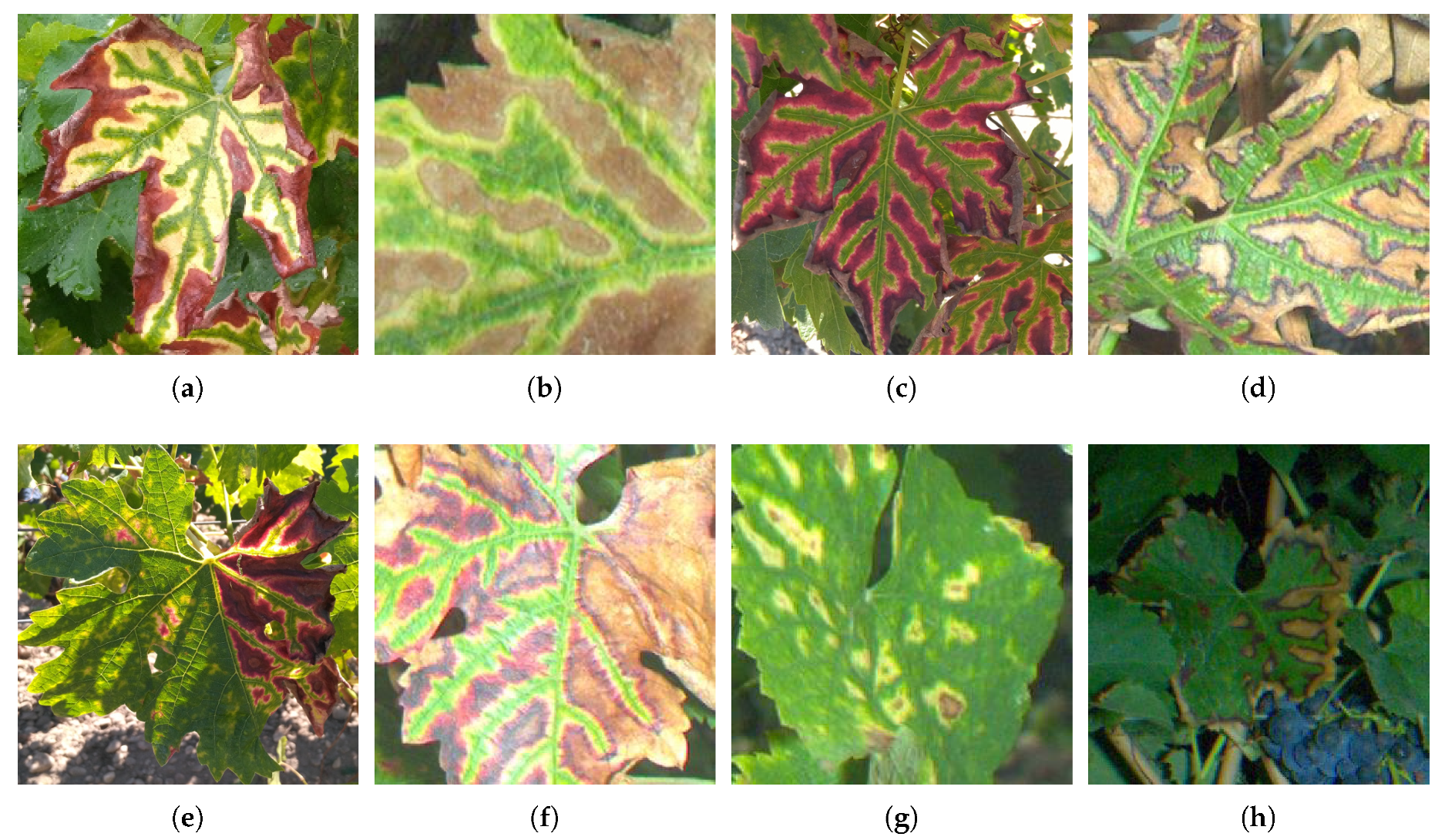
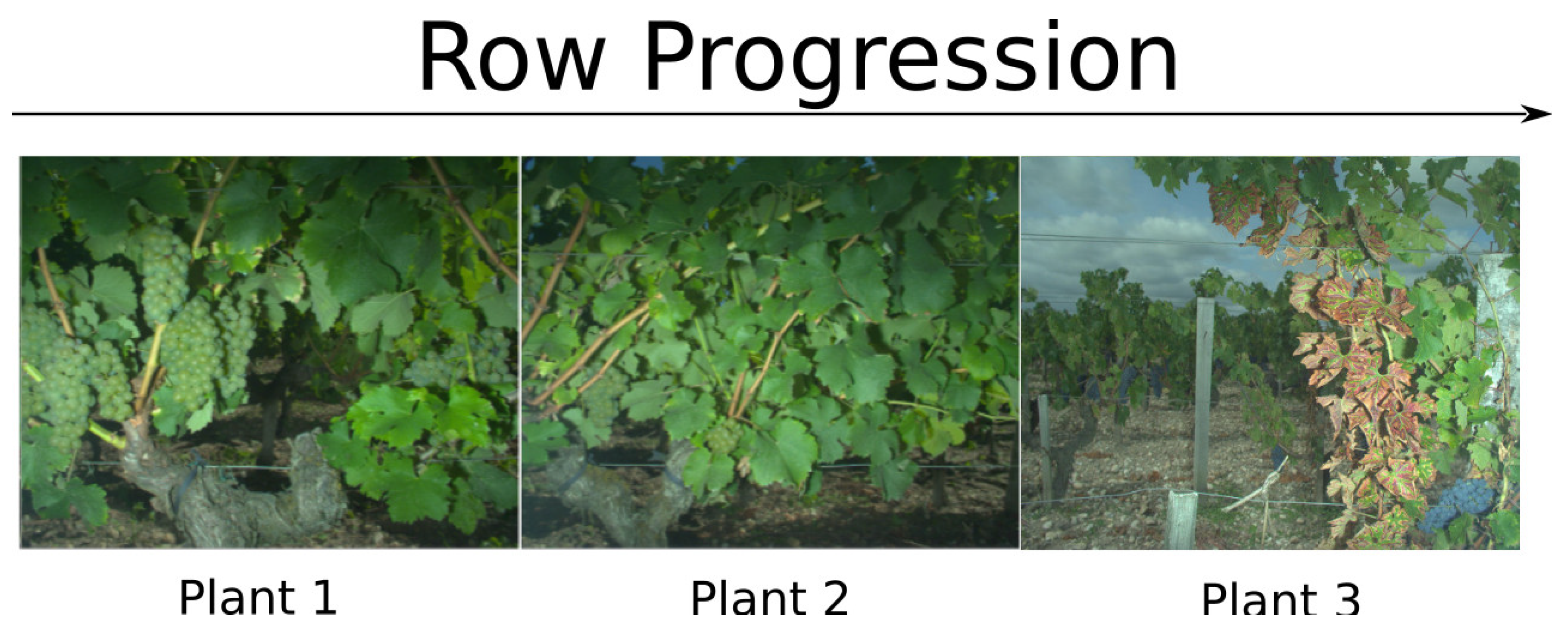
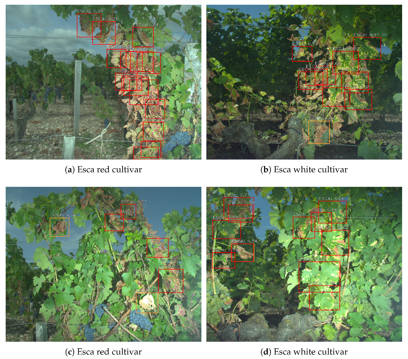
Esca foliar symptoms exhibit a particular pattern allowing in many cases accurate disease diagnosis. For instance, red cultivar esca symptoms appear as red spots turning yellow or necrotic [1]. These spots follow the shape of the leaf’s primary and secondary veins, resulting in the well known tiger-stripe pattern and its green → yellow → red → brown color gradient (Figure 1a–d). However, symptoms tend to appear differently between white cultivars and red cultivars. White cultivars usually show a wide strip of chlorotic yellow tissues (Figure 1a,b) while red cultivars show a narrow yellow strip (Figure 1c,d). In the case of apoplexy, leaves quickly turn to a pale green and wilt in a few days. Wilting is however not specific to esca and could be related to many other issues.

Typical tiger-striped esca patterns are however not so frequent in the vineyard as most leaves found on symptomatic grapevines show attenuated patterns, appearing only partly on the leaf and with varying intensity (Figure 1e) or partly wilted (Figure 1f). Circular patterns can also be observed in some cases (Figure 1g,h)

A year after year cartography of symptomatic plants could help disease management in the long term, allowing better replacement cycles and specific treatments. However, in reality, the exhaustive location list of these symptomatic plants is unknown. The random expression of yearly symptoms renders disease tracking even more confusing. Vine growers are usually unable to keep data of vineyard evolution between years. The only known solution is plant-by-plant human notation, a time-consuming task prone to errors (missed plants, symptoms appearing on one side of the row only, etc.).

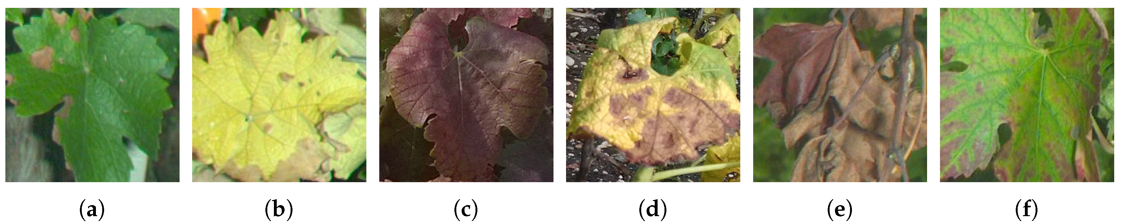
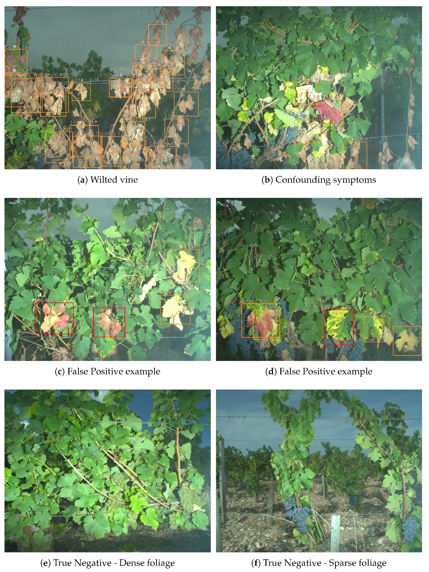
These issues motivate for the conception of an automated esca detection device, which may prove to be a significant challenge. Indeed, the presence of wilting, reddening and yellowing zones on the limb is not specific to esca. Actually, most grapevine diseases and deficiencies involve similar colorations, only the spatial patterns of these colors are different. Powdery Mildew/Black Rot (Figure 2a), Flavescence Dorée (Figure 2c-d), wilted leaves (Figure 2e), deficiencies (Figure 2f) and insect damages are among the other confounding factors found in the vineyard.

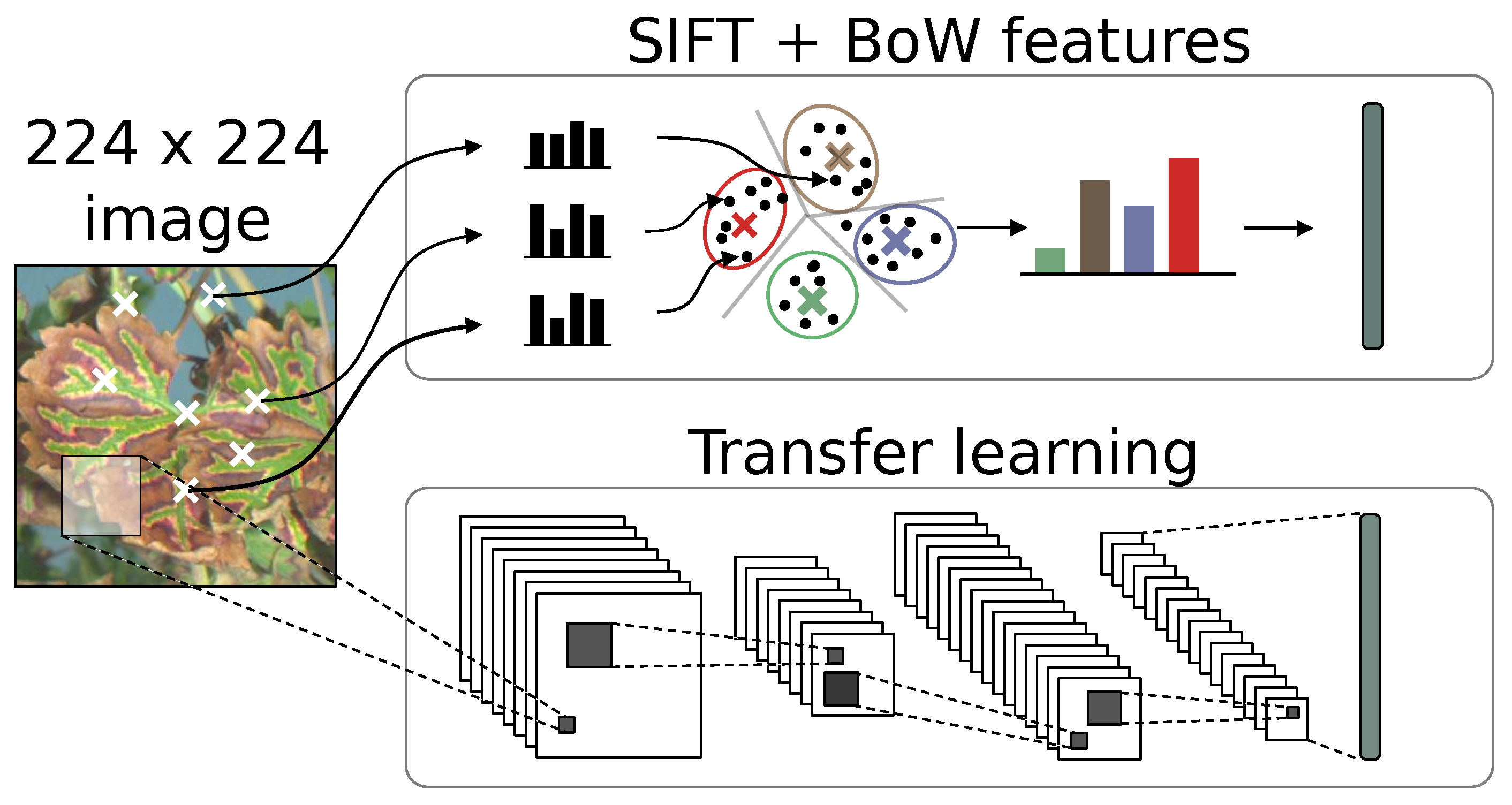
Sensors and computer vision are strong candidates to answer these questions in a non-destructive and automatic way. Another inherent advantage of imagery is that it allows a localized diagnostic in the plant, only pointing the symptomatic areas and quantifying the symptomatic portion of the plant. Huge improvements in the field of image analysis these last 15 years brought new promising tools for a great variety of tasks involving agriculture, which are referenced in numerous recent reviews [5,6]. More notably, deep learning methods have become increasingly popular, motivating a comparison between that novel state-of-the-art approach and more classical ones. These enhancements are used in this paper in the form of Scale Invariant Feature Transform (SIFT) based encoding and pre-trained deep learning convolutional neural network, allowing to generate sets of features describing in a compact way the composition of grapevine plant images. Thus, the main contributions of this paper are:

• the comparison of those popular methods in modern Content-Based Image Retrieval (CBIR) [7] applied to a specific and challenging plant disease problem, from leaf classification to detection of the disease at the plant scale; and
• the evaluation of the ability to discriminate esca samples from other leaf symptoms. Esca samples are also divided into three severity subclasses (used during the testing stage) to assess the performances on easy and hard samples.

This paper is divided into four main sections. Section 2 describes related works about computer vision methods and examples of agricultural applications. Section 3 describes the experimental design and image labeling steps leading to the creation of a custom database. In Section 4, we tackle the classification of leaf image patches from the databases, using the two distinct above-mentioned feature extraction approaches. Finally, Section 5 addresses the plant-scale detection problem on the basis of the classification step.

2. Related Works

Imagery using airborne or ground cameras is a popular choice for the detection of diseases or plant stresses in the field, whether it uses visible, multispectral [8], hyperspectral [9], thermal [10] or fluorescence [11] imagery. In-field esca detection is mainly studied using aerial multispectral imagery [12]. In this work, multispectral aerial imagery allows exhaustive vineyard cover and brings rich spectral information but suffers from geometric problems (stitching of images from different viewpoints) and lacking resolution for precise symptomatic leaves imaging. Differentiation between esca and flavescence dorée, another threatening disease with similar foliar symptoms, is also considered in some works, showing a will to differentiate target disease from other diseases [13,14]. The latter uses a combination of hyperspectral measurements and RGB imagery with textural analyses, in laboratory conditions. RGB imagery may seem less attractive at first glance but is actually a cost-effective choice. While it does not include rich spectral information (three-channel broadband sensor), spatial information may be used for disease detection problems involving symptoms with defined patterns, such as esca. We chose to study the problem using proximal sensing to propose a complementary application to remote sensing surveys.

The most simple image processing methods regarding disease detection are image binarization ones, considering a threshold to separate green (healthy) elements from the symptomatic parts, e.g., the work in [15] estimates virulence of wheat pathogen and compares it to traditional visual estimate methods. For that, colorspace transformations may be applied, such as RGB to HSV transformation (keeping hue information in a single channel) or vegetation indices (greenness index). Morphological operations can also be used to smooth the results and reduce false detections. These approaches are quite limited for more complex applications since they are sensitive to natural conditions (lighting, angle, shades, and organs with similar colors). Because of the absence of spatial information, they also perform badly if the underlying goal is to differentiate between diseases with similar discolorations.

Facing the limitations of color thresholding techniques, spatial information extraction was considered, taking into account the spatial relationships between pixels at first, and then between shapes and objects. Circular Hough transform was used as a powdery mildew spots detector [16]. Segmentation [17] allows retaining homogeneous spatial regions and then classify them according to the contained color features. Texture analysis, using for example standard Haralick indices, computed on gray level co-occurrence matrices, can also naturally be used and combined with other color features [18].

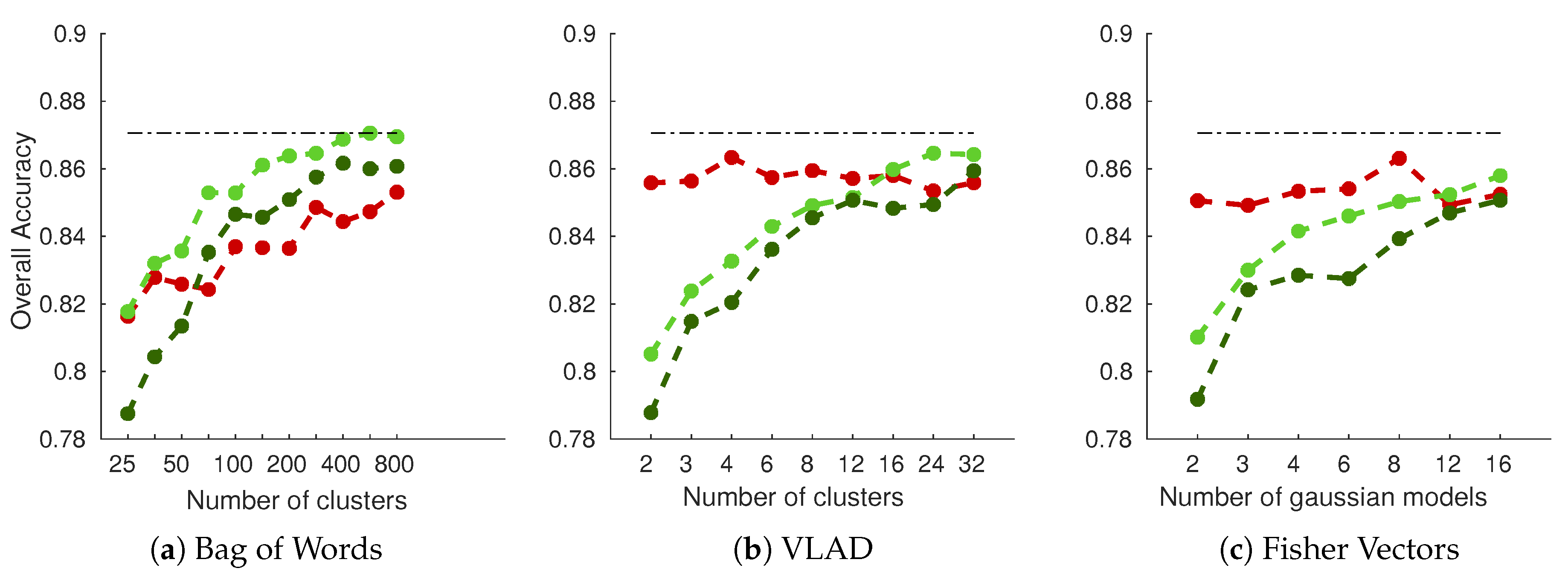
Lately, techniques naturally encoding the object composition of the image have been devised, allowing huge progress on general image classification tasks. SIFT keypoint detection is a powerful method used both for image classification and image correspondence [19]. The intuition behind SIFT relies on finding “keypoints” in an image and then computing a 128-dimensional descriptor around that point to summarize local gradient histograms information in a scale and rotational invariant way. That wealth of local informations can then be aggregated into a compact image representation using bag of visual word-type approaches [20]. SIFT descriptors are used for diverse agricultural applications such as leaf species classification [21]. In that case, the descriptors help to distinguish species based on the architecture of leaf venation and shape. In [22], species retrieval from a database of roughly 80 species is performed, using a fusion of several features including SIFT and Gabor filter, using HSI colorspace. A smartphone leaf identification system is devised for portable android device in [23] using SURF (a fast SIFT variant) features with bag of visual words. Similarly, rice flowering steps can be detected using the same SIFT descriptors [24]. Spatial grids of SIFT descriptors is also used in that study. As for disease detection, a set of three soybean diseases are classified in [25] on scanned leaves. Best results are achieved using a multiscale grid in the form of the Pyramid Histogram of Words (PHOW) method. Extensive experiments around SIFT variants (including color fusions and different keypoint detectors) are also performed in [26] for the classification of flowers pictures from three datasets. In the case of esca detection, SIFT/Bag of Words (BoW) combinations are of particular interest. Esca symptoms can be summarized as local patterns on the leaf (following the five main veins) with oriented soft gradients at different scales, meaning SIFT descriptors are good candidates to extract that information. On the other hand, BoW describes the composition of complex images with many objects and shape, similar to natural grapevine images. Other techniques based on local descriptors such as Local Binary Patterns [27], Gabor Wavelets [28], Histogram of Gradients [29] and structure tensor [30] are also popular methods in the literature.

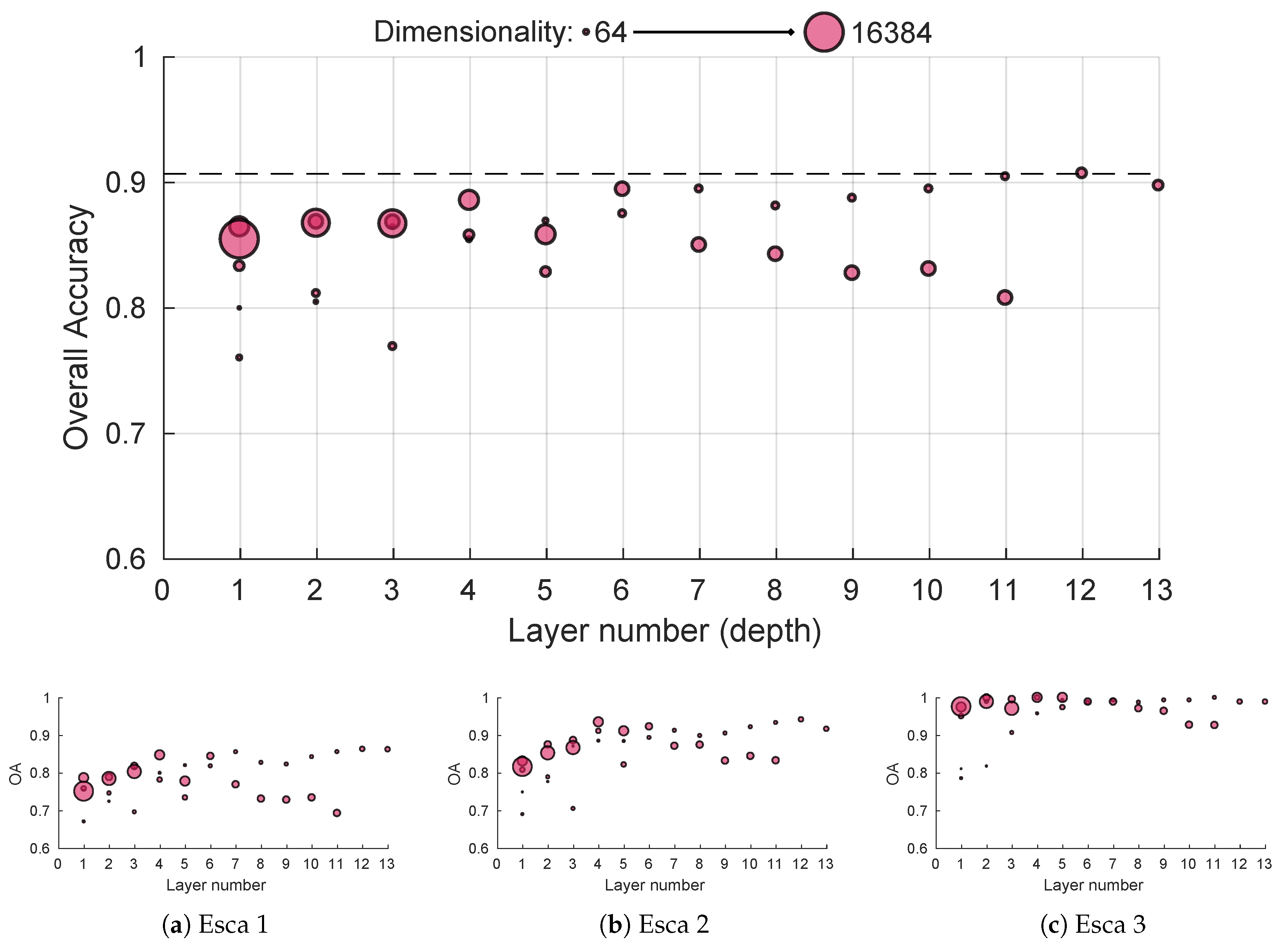
Deep learning methods introduced a new shift in the way we envision features. Convolutional Neural Networks (CNNs) architectures use a network of image filters to extract features from an image [31]. The weights determining the nature of these filters are learned during the training step. The user only defines the global structure of the CNN. CNNs are successfully used for image classification [32] and detection problems [33] on huge image databases (e.g., CalTech101 and Imagenet). The excellent results on these datasets have motivated the use of deep learning for many agricultural applications. For instance, plant identification is performed in [34]. In that study, two image databases are considered, one being the above-mentioned Flavia dataset and the other a custom database of smartphone images in natural conditions. In [35], the authors used VGG and AlexNet CNNs for classification on the Plant Village dataset. This database comprises images of different diseases and species in laboratory and infield conditions. It is worth noting that the network trained on laboratory images does not seem to generalize well on real field images. Web images can also be gathered to create a plant disease database such as in [36]. Using more advanced frameworks, Fuentes et al. performed the detection of tomato diseases using ResNet classification network and Faster R-CNN detection architecture [37]. In that paper, a data augmentation process is used to generate more samples based on variations of existing samples and reduce the overfitting effect. Fruit detection is also tackled in [38], merging RGB and NIR Imagery, exhibiting good detection results even for partially occluded fruits. Sometimes authors also try to deeply modify existing methodologies, e.g., in [39], the LeNet-5 network is used in combination with a novel k-means based weight initialization in order to improve classification performances of different weeds type in a soybean field and, in [40], a custom network is devised for the quantification of maize tassels on in-field images. CNN’s state-of-the-art performances on many applications motivated the use of deep learning techniques for esca detection.

From these works, several tendencies can be noticed:

• Image databases tend to grow bigger and to be more diverse. In parallel, laboratory studies in controlled conditions evolved into field condition acquisitions. Classification and detection problems are getting harder but in the meantime they are closer to potential commercial applications.
• Feature extractors become less and less specific. Many agricultural applications actually do not use ad-hoc approaches. Thanks to transfer learning, very general trained feature extractors can be efficiently used for specific tasks.
• Classifier importance has been revised downwards. State-of-the art classifiers such as SVM, random forest or artificial neural network provide satisfactory results that almost entirely depend on the two above-mentioned points. This means that, in most cases, noticeable performance gaps can only be achieved using larger databases and better feature extractors.

3. Data Collection and Processing

In field data collection was performed during summer 2017, in mid-august. Two plots from the Bordeaux region of France were used at the basis for the experiment: red cultivar Cabernet-Sauvignon vineyard in Pauillac and white cultivar Sauvignon-Blanc vineyard in Castres-Gironde. In both cases, the 50 first plants were sampled on even numbered rows. Since esca plants represent about 5% of the plants, esca samples are more sparse than healthy samples, thus additional plants presenting esca symptoms were handpicked to complete the database. Cartography of esca prevalence in the last five years was available, allowing to know in advance which plants are diseased.

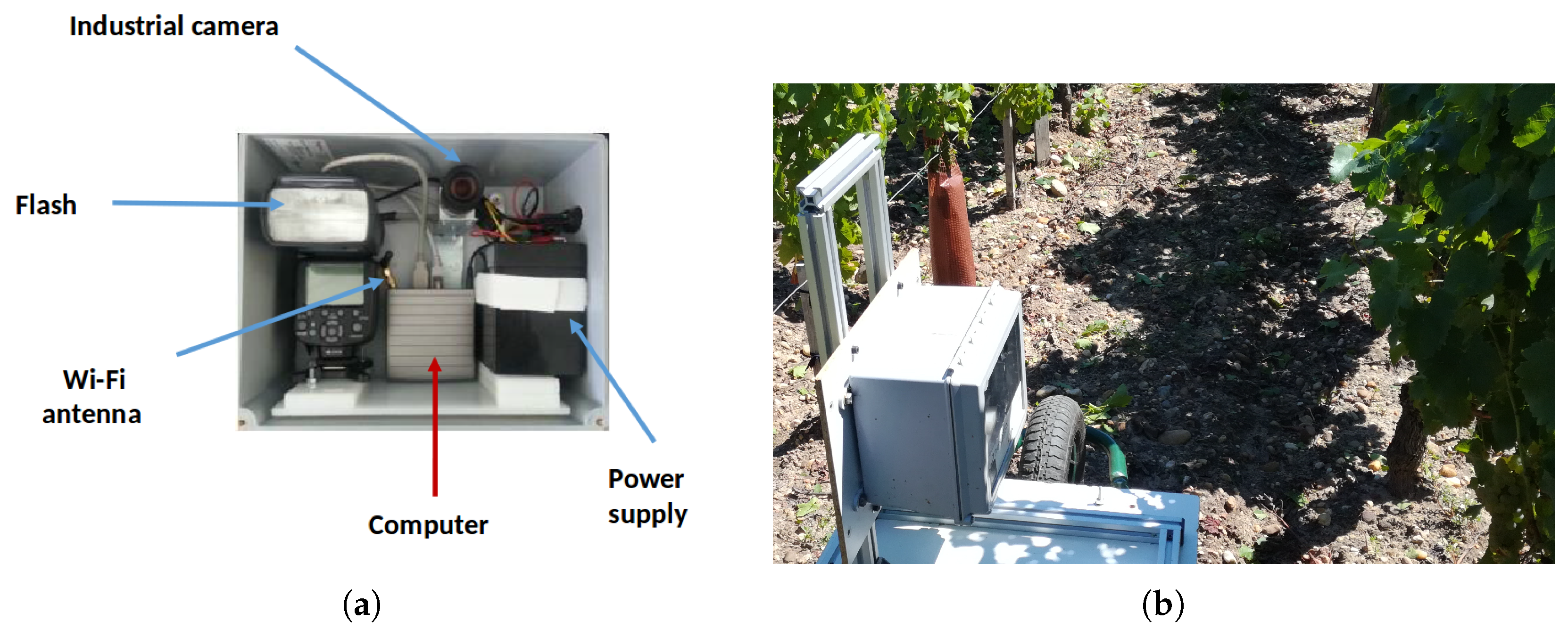
Images were acquired using a RGB 2592 × 2048 camera; the camera was protected in a sturdy box packed with a microcomputer (image storage and acquisition program) and an electronic flash (Figure 3).

Data acquisition was then triggered using a custom smartphone app for one-time acquisition or regular acquisitions. The device was then mounted on a transformed wheelbarrow advancing in the vinerow and aiming at the plants on the right side (Figure 4). This device could also be easily mounted on a tractor for fast and automatic acquisitions. Lens and flash calibration depend on natural conditions and thus were done on the field to obtain a clear image of the grapevine plant foreground with homogeneous lighting and blurry background (next vine rows). A picture was taken for each plant, centered as much as possible on the trunk. Spatial resolution of images is about 1 mm.

The differences in symptom expression shown in Figure 1 are greatly exacerbated by acquisition geometry and scene complexity. Leaves are visible at different angles and may be partially hidden. Esca symptoms are frequently overlain with stems, wires and other leaves. They may also appear blurry because of their relative position with the foreground, while the out-of-field background may trigger false positives. This means that the proposed classification algorithm should be robust to changes in illumination, rotation and obstructing elements. To take into account these differences, esca symptoms were roughly separated into three subclasses during the labeling process:

• Esca₃: Very well defined symptoms, most of the foliar area is affected, no occlusions (e.g., Figure 1a–d).
• Esca₂: Strong to medium symptoms (some parts of the leaf may not be affected), possible partial occlusions (e.g., Figure 1e,f).
• Esca₁: Weak symptoms or strongly occluded symptoms (e.g., Figure 1g,h). May be confounded with other diseases and abiotic stresses.

Since samples from these subclasses are scarce, these were only used during the testing stage as a way to evaluate more precisely the performances.

Image labeling was manually done using the free software LabelImg, outputting. xml files containing a list of bounding boxes for every labeled image. The files were then processed using a python script in order to create databases of rectangular leaf patches, which were then resized to 224 × 224 patches (

Table 1. Summary of image database samples: Number of 224 × 224 patches per class.

	Control	Esca			Confound.	Total
		Esca 1	Esca 2	Esca 3
White Cultivar	1554	326	165	43	630	2718
Red Cultivar	2045	259	218	60	953	3535
Total	3599	585	383	103	1583	6253

) during the feature extraction step.

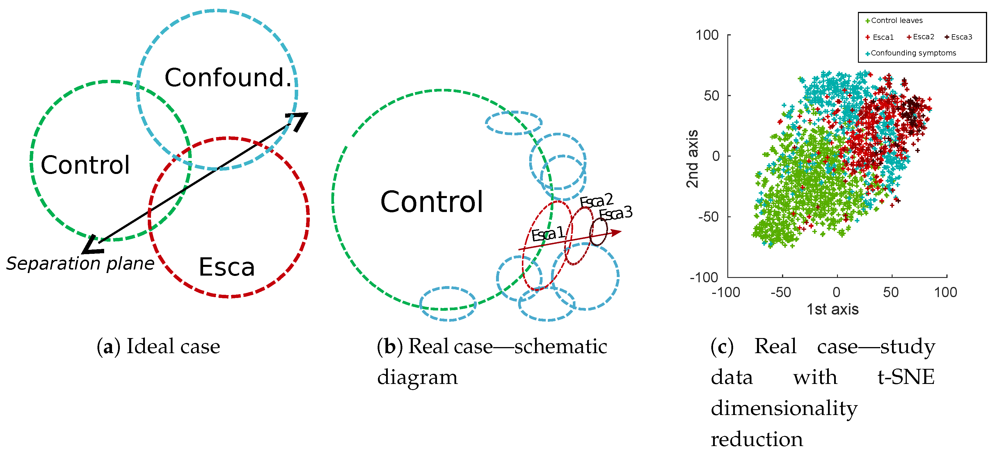
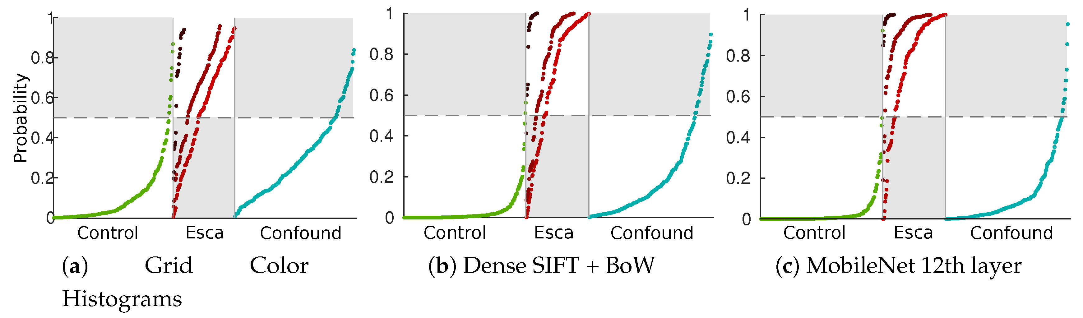
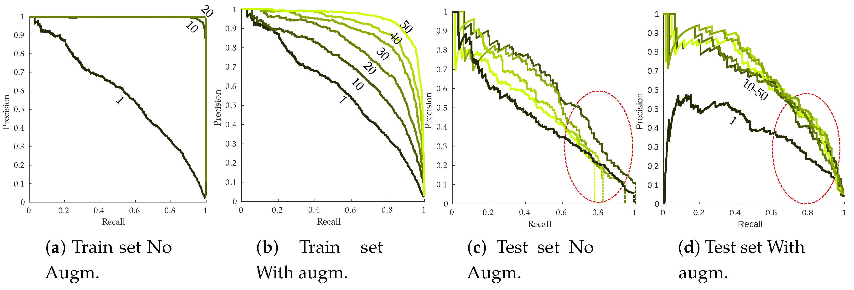
Natural class unbalance is easily noticeable, which can be explained by the low prevalence of esca symptoms in vineyards compared to the huge amount of control plants. It is also obvious that most of labeled esca symptoms are not “textbook examples” symptoms. Very well-defined symptoms are actually sparse, roughly 50 samples per cultivar in our database, which is not only caused by actual symptoms themselves but also by acquisition geometry. More generally, in real applications, background samples are often numerous, while targeted disease are scarce and present with varying intensity (displayed with green and red circles in Figure 5). Confounding factors (blue circles in Figure 5) could be separated in many different subclasses but most of them would have very few samples. In some cases, these subclasses are likely to be confounded with targeted esca class in the feature space (deficiencies) and in some cases not (powdery mildew, wilted leaves). A 2D visualization of features extracted from the database using t-distributed Stochastic Neighbor Embedding algorithm (t-SNE) algorithm can be found in Figure 5c. The t-SNE is a non-supervised dimensionality reduction technique known for its ability to find relevant embeddings in high dimensional spaces [41].

4. Leaf-Scale Classification

4.1. Methodology

Leaf classification consists in learning a model to predict which of the three classes a given leaf belongs to. Before learning the rules leading to prediction, features describing the leaf have to be extracted.

4.1.1. SIFT Descriptors

Scale-Invariant Feature Transform (SIFT) [19] is commonly used to describe local regions from an image in a scale and rotational invariant way. Most of the time, SIFT refers to a two-step process including keypoints detection (using for example the Difference of Gaussian (DoG) method) and computation of SIFT descriptors around these keypoints. The first step can however be replaced by any other method such as Harris detector or a simple regular grid of keypoints. Given a keypoint (coordinates), its scale (defining the zone covered by the descriptor in the image) and the main dominant orientation of the gradient within that zone, local gradient histograms were sampled in eight directions on a 4 × 4 grid (examples of SIFT descriptor grids at different scales and angles are provided in Figure 6b). A 128-dimensional SIFT descriptor was then formed by aggregating the 16 histograms of gradients in the grid. Finally, normalization is often applied on the resulting vector. The resulting features are known to be scale and rotation invariant, which means that a rotated and scaled image should provide very similar SIFT features than those computed on the original image. For classification tasks, it allows more robustness to these changes. Interestingly, in the case of standard keypoint detection only, healthy leaves samples yield significantly less keypoints than symptomatic leaves, which makes sense since keypoints mainly react to leaf veination and edges while symptoms also trigger many other keypoints at different scales, as illustrated in Figure 6. Keypoints position, scale and main orientation are displayed in Figure 6a while examples of individual descriptors (orientation histograms within cells of a 4 × 4 grid) built on these keypoints are displayed in Figure 6b.

In this study, performance of DoG + SIFT approach was evaluated, along with two other sampling strategies:

• Dense SIFT, in which keypoints are sampled on a grid at fixed scale and orientation. Step and scale parameters were chosen on the basis of a preliminary grid search experiment. Grid step was fixed to 4 pixels while scale parameter was 5.
• PHOW SIFT [42], an extension of Dense SIFT using a multi-scale grid. In this experiment, the proposed SIFT scales were $[4,8,12]$. Grid step was augmented to 8 to reduce the size of the resulting descriptors and prevent memory issues during the training step.

4.1.2. Feature Encoding

While the computed SIFT local descriptors are informative on their own, they do not provide a compact representation of the image. Since the number of extracted descriptors may vary between images, direct comparison between them is not possible. Bag Of Visual Word (BoW) [20] was developed to create a vocabulary of descriptors (called visual words) that best describe the image. It can be summarized in 2 steps:

• Unsupervised clustering (most of the time using k-means) is performed in the descriptors space so that families of similar descriptors are grouped. This leads to the creation of a dictionary of k words, a list representing the diversity of descriptors in the learning database. In that step, common grapevine elements at different scales are learned.
• Image encoding is then applied to a test image. SIFT descriptors are computed and assigned to the nearest cluster/word in the descriptors’ space. Frequency of appearance of each vocabulary entry then allows us to construct an histogram of fixed size (k) describing image composition.

Vector of Locally Aggregated Descriptors (VLAD) [43] addresses the main problems inherent to BoW method, namely the lack of weighting. As in BoW, each descriptor is assigned to its nearest cluster, and then, for each cluster, we consider the sum of differences between assigned descriptors and the centroid of the cluster in the SIFT 128-dimensional space. More discriminative property is thus achieved by using first order information in the process. The drawback to that information is the augmentation of the descriptor’s dimensionality, which can be critical for problems with small sample number. Fisher Vectors [44] (FV) enrich first order information with second-order statistics by substituting the initial k-means clustering step with a Gaussian Mixture Model (GMM) parameters estimation (means, covariance matrix and prior weights), with an expectation maximization algorithm. Similar to VLAD, first- and second-order statistics are then aggregated in the resulting FV. VLAD can thus be seen as a simplified version of FV. It is worth noting that the dimensionality of the resulting features does not depend on the total number of local descriptors in the training database or on the number of descriptors per image. However, these substantially affect the quality of representation if too few samples are available. As mentioned before, VLAD and FV dimensionality are two orders of magnitude higher for SIFT encoding (

Table 2. Dimensionality of encoded image features and range of k parameter tested in the experiments (k = Number of words/clusters/Gaussian models in the SIFT descriptor space).

	BoW	VLAD	FV
Dimensionality	k	128 × k	256 × k
Tested k values	25 → 800	2 → 32	2 → 16

). To alleviate the risks associated with high dimensionality, lower k values are used when considering theses approaches. VLAD and FV approaches are known to have very good performances using small dictionary size.

SIFT detection applies to single channels image, thus SIFT + BoW approach describes the composition of a single channel. To combine the information of several channel, fusion of features, after the encoding part, was performed. As recommended in the literature [44], an L2 normalization followed by square rooting was used for the three approaches.

SIFT keypoint detection and encoding algorithms were freely adapted from VLFeat toolbox, which provides useful functions for computer vision and machine learning in Matlab environment (Matlab R2017a) [45].

4.2. Deep Learning Approach

In the imagery field, deep learning often refers to convolutional Neural Networks (CNNs), which can be seen as a classifier on top of an automated feature extractor. CNNs are networks containing multiple layered image filters with multiple connexions between layers. The weights defining the nature of these filters are however not defined by the user but instead by the learning process, linked with a classification neural network (fully connected layers). Weights evolve during the optimization process so that a loss function is minimized. Several training strategies can be considered, depending on the application and the database:

• Full Training consists in training both the convolution and the classification part of the network. Full training is more appropriate for databases of sufficient size or simple applications.
• Fine-Tuning consists in training only part of the convolutional layers of a pre-trained network (trained on a huge database such as Imagenet). In this transfer learning method, shallow and general layers are kept frozen while deep layers are re-trained with a very small learning rate to learn features specific to the database. Fine-tuning generally works well for small databases.
• Feature extractor approach is a more direct case of transfer learning. It also uses a pre-trained network but directly treats it as a multi-usage generic feature extractor. No training is done on the convolutional part and feature map extraction can be performed at any level of the network. Based on these extracted features, any classifier could be used to obtain the final decision.

In this study, we chose the feature extractor approach as the comparison basis with SIFT features, since it is an adapted solution for small datasets. Using pre-trained general feature extractor allowed us to evaluate the viability of transfer learning on our very specific application. Since we treated feature extraction as a bottleneck, the same classification strategy and framework could be applied for both SIFT and deep learning experiments (Figure 7).

4.2.1. Convolutional Network Choice

In many studies, network choice is motivated by a trade-off between speed and accuracy often linked with the network’s depth and the input image size. Deeper networks usually yield better results on more complex image sets at the cost of lower speeds and with more demanding GPU memory consumption. The number of parameters in the network is however not necessarily correlated with the depth of the network. VGG16 is an example of a relatively shallow network with a huge number of parameters beneath. Recent networks may also introduce new building blocks in the convolutional structure, such as ResNet50 using residual learning to compensate for gradient dissipation problems in deep neural nets. In that study, we chose to use the lightweight MobileNet family [46] as the convolutional basis. MobileNet is an adaptable family of networks using 13 convolutional layers (each containing a full set of filters) generated by two parameters: input image size and network depth $\alpha$. Every element of the MobileNet family was trained on ImageNet database, providing a set of ready-to-use networks for different applications. MobileNet can also be easily embedded on mobile platforms. This is particularly interesting in the case of this study because the long term goal is tractor-mounted real time acquisition and processing. Here, we considered the default MobileNet for our application, using standard 224 × 224 input size and $\alpha =1$ for a network of approximately 4 millions parameters. This network has proved its efficiency notably on the Imagenet database, on which it reached a Top-5 accuracy of about 87%.

4.2.2. Feature Extraction on Pre-Trained Network

Feature maps obtained using the feature extractor approach can be used in different ways, mainly depending on two parameters:

• Network Depth. Every convolutional layer output can be used as the final feature map. First layers tend to capture low level information (mainly edges and color filters) while last layers tend to encode more complex spatial relationships such as shapes, parts and objects
• Pooling Strategy. Feature maps are multi-dimensional arrays, implying the need for a post-processing step before flattening and feeding them to a classifier. CNNs often use max pooling or average pooling techniques, or even a combination of the two. Output feature maps tend to be sparse so max pooling may be the best choice in most situations.

The many possible combinations of network depth and pooling strategy create final features of different natures and dimensionality, as shown in

Table 3. Resulting dimensionality of grid pooling strategies on convolutional layers outputs.

Layer [Output]	1 × 1 (global)	2 × 2	4 × 4	8 × 8	16 × 16
Conv1 [112 × 112 × 64]	64	256	1024	4096	16384
Conv2/3 [56 × 56 × 128]	128	512	2048	8192	.
Conv4/5 [28 × 28 × 256]	256	1024	4096	.	.
Conv6/7/8/9/10/11 [14 × 14 × 512]	512	2048	.	.	.
Conv 12/13 [7 × 7 × 1024]	1024	.	.	.	.

. Pooling is performed using five different grid sizes, maximum values for each cell of the grid and for each channel are then flattened to construct the final descriptor. For instance, Conv1 output (64 channels) with 2 × 2 pooling yields a 256-dimension descriptor.

Deep learning feature extraction was performed using Python 3 and the Keras/Tensorflow framework, allowing an easy access to pre-trained models on the ImageNet database.

For both experiments, preprocessing simply consisted of an image standardization (zero mean and unit variance). This step is done automatically using the Keras framework for the deep neural network and was implemented in Matlab for the SIFT based experiments.

4.2.3. Classifier Choice

In this study, we chose the conventional Support Vector Machine (SVM) classifier, which, on preliminary tests, gave better results than other well-known classifiers such as Random Forest or K-Nearest-Neighbors. Distance matrix was computed to use the ${\chi }^2$ metric for BoW experiments and Euclidean distance for other experiments. Radial Basis Function kernel was then used on the matrix before training a linear SVM using libSVM library. Training and testing were performed on separate datasets. Partitioning of the dataset was done using a set of 10, randomly pre-generated, 50%/50% train/test splits with balanced number of samples per classes. That way, the same train/test splits were used for the compared experiments. A 10-fold cross validation was also used during the SVM training. Ten percent of the training set was randomly used for the validation set to tune the $\sigma$ parameter of the RBF kernel.

4.2.4. Evaluation Metrics

The overall accuracy was considered as the evaluation metric on the test set. Overall accuracy summarizes accuracy for all classes, which is the proportion of samples assigned to the correct class. Overall accuracy is also in that case the non-weighted mean of class accuracies since all classes are balanced in the generated test sets. Esca subclass accuracy can be simply defined as the proportion of a given subclass sample being assigned to the correct class, for example the proportion of leaves heavily affected by esca correctly classified as esca. Following the probabilistic SVM approach [47], posterior probabilities can also be extracted for the samples in the testing step to get an estimate of the classifier relative confidence for each decision.

As a complimentary measure to overall accuracy, two other indicator were introduced. First, Matthews Correlation Coefficient (MCC) can be seen as a balanced measure similar to the ${\chi }^2$ statistic on a binary contingency table (the confusion matrix).

$$\begin{array}{c}\hfill MCC=\frac{TP\times TN-FP\times FN}{\sqrt{(TP+FP)\times (FN+TN)\times (FP+TN)\times (TP+FN)}}\end{array}$$

(1)

which ranges between −1 and 1, the former being a totally incorrect classifier and the latter a totally correct classifier. Pairwise coefficients for binary cases are averaged in order to obtain multiclass MCC.

Then, to compare competing experiments and determine whether the difference is significant, one can also use the McNemar test [48]. Using a contingency table between two classification prediction results, the H0 null hypothesis indicates probabilities of each outcome are the same while the H1 hypothesis indicates they are not. If the H0 null hypothesis is true, the statistic should follow a ${\chi }^2$ distribution with a single degree of freedom.

4.3. Results

4.3.1. Performances of Simple Color Based Methods

We compared the performances for our two approaches but also for two other simple color-based methods. Color histogram method simply considers the global image histogram as the final feature. Various bin sizes and color fusion strategies (in the form of concatenated histograms) were experimented to get the best result. An overall accuracy of around 75% (respectively, 74.4% and 74.9% for white and red cultivar datasets) was achieved using that method, meaning a decent part of the samples can be actually well classified using the most simple approach, which is not surprising. Most of the well classified samples are from the control class (about 88% class accuracy) while esca and confounding factors class are harder to classify (respectively, 65% and 67% class accuracy), showing difficulties to differentiate symptoms. In an effort to use spatial information, grid of color histograms considers a spatial grid laid on the image, and then a histogram is computed within each cell of the grid. Local histogram are then either concatenated or encoded using the three methods presented in this paper (BoW, VLAD, and FV). In the best case, this yields a gain of around 5% of good classifications compared to simple color histogram approach, meaning the base performance using grid color histogram approaches and channel fusion is about 80% (respectively, 79.7% and 80.4% for white and red cultivar datasets).

4.3.2. SIFT Performances

As shown in Figure 8 (results for RGB fusion on white cultivar dataset), performances are dominated by dense grid of SIFT descriptors encoded with simple BoW histogram, reaching around 87% accuracy. Performances are gradually increased with the number of clusters for BoW encoding. That does not hold true for VLAD and FV encoding, however, in which only grid-based methods yield increasing performances, while DoG SIFT yields relatively stable performances. This is an interesting property of these two methods, since it means that good results can be achieved with small dictionary sizes. It is also interesting to note that single scale dense grid seems to perform better on all experiments than multiscale grid. This could be an un undesirable effect of the threefold augmented descriptor dimensionality. Similar interpretations could be drawn on the red cultivar dataset.

4.3.3. CNN Performances

While general CNN performances depend on the depth extraction, decent image representation can be achieved using only the first convolutional block, providing accuracies similar to the SIFT method using a trained set of 64 filters sensitive to edge and color with posterior max pooling (Figure 9). Performances seem to gradually improve with depth until the sixth layer; worst-case performances in case of inadequate pooling also seem on the rise (worst performance was above 85% and best one above 90% for block 6). For deeper layers, performances are more uncertain, although global best accuracy was achieved using global max pooling in the 12th block output. This could mean deeper layer features lack the generalization ability of more shallow ones. Interestingly, it seems high dimension features perform better on shallow layers while low dimension features perform better on deep layers. Things are slightly more different for the sub-accuracy scores. Typical esca symptoms get easily classified with near 100% accuracy for every depth in the network as shown in Figure 9c. However, shallow features tend to struggle on more subtle foliar symptoms, the fourth layer marking an important performance boost in more difficult symptoms classification (Figure 9a,b). Similar behaviors were observed for the red cultivar dataset.

4.3.4. Summary

While both studied methods provide similar results (best accuracies around 91% accuracy on white cultivar and 88% on red cultivar), deep learning features present the advantage of slightly better performances (

Table 4. Summary of best mean performances (%) for the whole dataset (OA), esca subclasses (esca1–esca3) and the confounding factors class (Conf) using 10 different train/test runs with balanced classes. Mean standard deviation for all results is around 1.6%. Bold values indicate best results for both extractor families. RGB, HSV and hue images were considered for SIFT based extractors and only the best result is displayed. Max pooling, average pooling and a combination of these two were also considered for deep learning based descriptors.

		White Cultivar					Red Cultivar
		OA	Esca1	Esca2	Esca3	Conf	OA	Esca1	Esca2	Esca3	Conf
DoG SIFT	BoW	85.4	80.1	82.7	97.6	79.5	83.4	82.2	92.2	100	74.1
	VLAD	86	83.2	88.1	98.8	81.1	83.6	83.7	94.1	99.2	75.2
	FV	85.7	82.4	85.6	98.4	81.4	83.2	82.5	93.2	97.7	74.6
Dense SIFT	BoW	87.9	82.3	90.2	100	81.1	85.4	85.9	90.8	99.7	76.7
	VLAD	86.7	80.1	91.6	99.8	82.4	82.7	81.3	89.2	96.3	75.1
	FV	86	82	89.9	99.2	80	81.5	82.2	88.4	96.5	72.5
PHOW SIFT	BoW	87.1	80.5	87.1	98.6	79.5	84.4	84.9	92.2	100	74.9
	VLAD	85.8	80	89.8	99.8	80.6	80.9	81.1	89.6	99.7	72
	FV	85.5	80.9	87.7	97.8	80.4	80	80.1	87.4	98.9	70.6
MobileNet 224-1.0 Imagenet features	1st layer	87.8	80.6	87.6	95.5	82.1	86.4	89.5	92.7	96.5	71.4
	7th layer	90.2	85.6	93	99.3	85.9	86.4	92.7	97.8	100	76.1
	12th layer	90.7	86.3	94.2	98.9	86.9	87.8	92.1	98.3	99.8	78.3

) at lower parameterization costs. It provides significant enhancements in the classification of confounding factors: the most difficult class due to its extreme variability. Dimensionality seems to play a role in the classification performances, best accuracy being obtained with final features with around ${10}^3$ dimensions. While perfect classification seems hard, if not impossible, best features perfectly separated healthy leaves from symptomatic leaves (even in the most complex cases) and limited the number of other symptoms wrongly detected as esca.

Table 5. Overall accuracy and Matthews Correlation Coefficient (MCC) performance indicators on three selected experiments (white cultivar).

	Grid Color Histograms	Dense SIFT + BoW	MobileNet 12th Layer
Overall Accuracy (%)	79.7	87.9	90.7
MCC	0.69	0.76	0.84

presents a comparison of the performances for three selected experiments using overall accuracy and Matthews Correlation Coefficient (MCC). While similar behaviors are observed, it seems the gap between SIFT approach and deep learning approach widens using the MCC.

Using the McNemar test on the above-mentioned experiments showed the “MobileNet 12th layer” approach performed significantly better than the “Grid color histograms” and “Dense SIFT + BoW” methods (respective p-values were $\approx 0$ and 1.5 ×${10}^{-2}$).

The difference between weak features (using the best color histogram strategy) and strong features can be seen in Figure 10 using SVM posterior probabilities on the test set [47]. In that figure, sorted probabilities are plotted separately to visualize the repartitions for the three labeled classes (control, esca and confounding factors) and the three esca subclasses (darker reds indicate more defined symptoms). Grey zones indicate bad classification cases for a given class.

From these results, we can conclude that transfer learning approaches are a promising method for informative feature extraction related to esca (and possibly other diseases). Deep and intermediate layers outputs, combined with aggressive pooling (low resulting dimensionality) yielded the best performances on the MobileNet network. Next, the discriminative power of deep learning features was extended to disease detection on plant images.

5. Plant-Scale Detection

5.1. Methodology

Detection Network

Detection at the plant scale involves finding and classifying symptomatic leaves on a picture containing the full plant. This results in much harder blind search problems within complex images. A good detection network should output anchor boxes and associated classes fitting the human annotations. Detection algorithms have drastically evolved during the last 15 years; their evolution can roughly be summarized into three main steps:

• Standard Sliding-Window approaches, in which each window is fed to the trained CNN. This is the slower approach.
• Two-Step Detectors, using a Region Proposal Network (RPN) to get anchor boxes and then feeding the proposal to the trained CNN (R-CNN and Faster R-CNN).
• One-step Detectors, in which both processes are done simultaneously, using dense sampling (YOLO, SSD, and RetinaNet).

Among these three, the last two are the most used nowadays. Actually, these strategies represent a trade-off between speed and accuracy, two-step network providing state-of-the-art accuracies and one-step networks providing fast inference (brought by the need for real time applications at several frames per second). Recent detection networks use a trained CNN such as MobileNet, ResNet or VGG as the feature extractor backbone. RetinaNet [49] uses anchor boxes in the same fashion as the enhancements of the Faster R-CNN network. It combines a regression subnet and a classification subnet (4 3 × 3 convolutional layers) applied on pyramid of features at different depths [50] (Figure 11). Each pyramid element has its own output and is fed to the regression and classification head. Multi-scale anchors are proposed for every feature level with different aspect ratios. In that case, RetinaNet uses 15 anchors types over each element of the pyramid. The known problem with one-stage detectors using dense sampling is that they fall short in terms of accuracy compared to two-stage partly because of class imbalance during training. Thus, heavy presence of easy negative samples (in our cases healthy leaves) may overwhelm the detector. To overcome that issue, RetinaNet uses focal loss. Focal loss consists in a change in the cross entropy function, allowing to give less weight to easily classified background zones of the image, summed on every anchor of the image. On the contrary, hard cases are given large weights during the training. Predictions from all feature pyramid levels are then merged using standard non-maximum suppression (NMS).

RetinaNet was thus applied using the same MobileNet backbone as in the previous experiments. As mentioned above, the goal of the backbone is to compute rich multi-scale feature maps over the whole image which can then be fed to the subnetworks dedicated to classification and regression. In that regard, previous experiments on leaf classification are useful to ensure the feature extraction part is relevant. Trunk and grape classes were also added to the database to take into account these natural organs present in every vineyard.

5.2. Parameters of the Experiment

Performances were evaluated with respect to two main parameters: image size and data augmentation. Image size is a crucial parameter in the speed/accuracy balance. We thus tested different input image width: 500, 1000 and 1500 pixels. On the other hand, data augmentation enriches the training database by applying various transformations to images during the learning process at each epoch. Data augmentation is known for performance boosts and overfitting limitation for datasets with few samples. In the experiment, we consider whether using data augmentation. Data augmentation consisted of random geometrical transformations, including images rotations, resizing, shearing and random flips.

As for the training parameters, Adam optimizer [51] was used with a learning rate parameter of ${10}^{-5}$ and 50 epochs (however, due to overfitting during late epochs, predictive model at Epoch 20 was used as the basis for the later detection examples). Batch size depends on the input image size; bigger images need smaller batch sizes in order to not overwhelm GPU memory (GTX GeForce 1060 with 6Go memory).

5.3. Evaluation Metrics

Image search problems work differently from classification problems. Classification associates an image with a label while detection associate an image with a variable number of bounding boxes and labels. Here, we used the common Recall/Precision indicator to evaluate the segmentation quality. Recall (R) indicates which proportion of annotations (bounding boxes) our trained algorithm is able to detect while precision (P) indicates the accuracy associated with this recall (proportion of true positives in the detections assigned to the class). This can be formulated as a function of true positives (TP) and false positives (FP):

$$\begin{array}{l}R=\frac{TP}{N}\\ P=\frac{TP}{TP+FP}\end{array}$$

(2)

where N is the number of actual annotations in the class. Varying the classification score threshold allow us to construct the RP curve. From this latter, average precision (AP) for a given class can be computed as a weighted sum of precision values through possible recalls:

$$AP=\sum _{i=1}^N(R_i-R_{i-1})P_i$$

(3)

where i is the position on the RP curve or in other terms the threshold index in the sorted scores vector (easy high-scored samples are recalled first while hard low-scored samples are recalled last). Most of existing detection benchmarks consider mean AP values along all classes. However, we only used in the results the AP metric for the esca class since we are only interested in esca detection’s performances. Assignment of an annotation box to a detection box is decided using the intersection over union (IoU) value between the two rectangles. IoU = 0.5 threshold was used in this study. Train/test split was performed using a set of 1133 images for training and 141 images for testing. Testing set was designed so that it is representative of the diversity of hard/easy esca and confounding factors cases. Image repartition is detailed for the detection task in

Table 6. Repartition of plants in the training and the testing database in the detection framework. Percentages do not necessarily add to 100% since some plants can have both esca symptoms and other symptoms.

	Number of Images	Images with no Symptoms	Images with Esca Symptoms	Images with other Symptoms
Training	1133	669 (59%)	170 (15%)	353 (31%)
Testing	141	43 (31%)	25 (18%)	78 (55%)

:

5.4. Results

5.4.1. Detection Examples

Once the whole detection network has been trained, it can be used for inference on new images that did not participate for training. Examples of detections on esca plants can be found in Figure 12 for both cultivars. Esca is detected using red frames while other symptoms are detected using orange frames. Only esca and confounding factors classes were represented since healthy leaves, grapes and wood are background classes. As expected, well defined symptoms are easily spotted with good confidence rate though some difficulties remain for more challenging areas. While detection of isolated leaves is easy, zones with many overlain leaves are sources of errors. Depending on the situation, detections may only cover a part of a leaf or a group of overlapping leaves. Both are actually correct, which is why the original dataset was labeled in both ways. Leaves with bad contrast are most of the time recognized such as in the upper left corner of Figure 12d. Stems, wood, soil and background do not trigger false positive detections.

As for other symptoms, totally wilted vines such as in Figure 13a do not seem to trigger false detections (although wilted vine may indicate esca apoplectic form). Some false positives remain however for symptoms closely related to esca, such as in Figure 13c,d. Healthy leaves, which have dense or very sparse foliage do not trigger false detections as well (Figure 13e,f). Scores are typically higher for esca symptoms than for other symptoms (meaning score threshold may introduce false negatives for the latter class). This is not surprising since that class is not as specific as the esca class and thus the network may have not learned a specific signature but a wide range of signatures of symptomatic leaves that do not fall in the esca class.

5.4.2. Recall–Precision Curves

Figure 14 presents the RP curves for the training and the testing set as well as the effect of data augmentation on detection performances. Without data-augmentation, overfitting is strongly noticeable on the training set (Figure 14a). Perfect RP metrics are already reached by the end of the first 10 epochs, meaning every annotation is detected with high confidence scores. Meanwhile, test sets RP curves are strongly lagging behind. This kind of behavior is not desirable since the network should not learn rules specific to the training set. Effect of simple data augmentation can be easily seen, with more progressive training that does not end with perfect performances (Figure 14b), although there is still a noticeable gap between training and testing performances. It is worth noting that performances seem to degrade during the last epochs, stressing the need for early stopping of the algorithm. Symptomatic leaves easier to recall (most likely leaves from the $esc{a}_3$ or $esc{a}_2$ subclasses) are retrieved with similar precision when data augmentation is used or not. More difficult leaves however seem to strongly benefit from data augmentation, with a slower precision decay (as indicated by the red circles from Figure 14c,d). Using a 75% recall, base algorithm yielded approximately 40% correct detections while this number jumped to 60% using data augmentation. A side effect of overfitting can be seen in Figure 14c. Maximum achievable recall on test dataset drops throughout the epochs (indicated by the dotted vertical lines). For the 50 epochs mark, less than 80% of the annotated symptoms are recalled, even using very low classification threshold. Over-specific models tend to ignore these kind of samples. Data augmentation fully resolves the issue, maximum recall being close to 100% even at the end of the 50 training epochs (Figure 14d).

AP curves presented in Figure 15 show similar behavior on training and testing sets. A significant gain of about 20% in the best case was observed when data augmentation was considered. In that case, getting higher AP values is difficult since for high detection thresholds the many hard labeled samples may not be detected (false negatives). Note also that some detections may not have been labeled (false positives), which is linked to the challenge of creating the annotation database. Image size seems to play a minor role on performances except for the 500 pixel width images which yield significantly lower performances. While data augmentation is a great tool to compensate for small databases, it cannot bring new information. Larger and more diverse databases will always be preferred to data augmentation but this latter seems sufficient for our application. As mentioned above, to compensate for overfitting on the training set, learning phase termination was set to 20 epochs (dashed red line on Figure 15).

5.4.3. Esca Intensity for Each Plant

Evaluation metrics presented beforehand are useful for assessing the quality of the segmentation but they do not take into account the fact detections may belong to the same image. Some plants are more affected than others and we need a quantitative estimation of symptom intensity for each plant. Thus, as a complementary tool to RP curves, we considered the relation between the annotated esca surface per image and the detected esca surface (Figure 16). Figure 16a shows this relation on the training set and Figure 16b on the testing set with 0.5 score threshold.

Samples on the scatter plot origin are images without esca annotations that did not trigger an esca detection, which can be seen as a group of true negatives (TN). Similarly, samples on the y-axis (red dots) are false positive (FP) samples and those on the x-axis (blue dots) are false negative (FN) ones. No false negative was observed on the testing set meaning every annotated esca plant triggered at least one detection. Test set resulted in seven false positive images (two of them are presented in Figure 13c,d, meaning detections occurred while nothing in the image was labeled as esca. Detected surface is however rather low in those samples, meaning these false positives would be labeled with low esca intensity. As for true positives (TP), decent correlation is obtained on the test set, meaning that it is possible to roughly quantify esca intensity for each plant.

5.4.4. Computation Times

Table 7. Computation times for a GTX 1060 GPU (6go memory).

Image Width	500	1000	1500
Learning time (hours for one epoch)	0.12	0.40	0.44
Prediction time (seconds for one image)	0.15	0.16	0.18

presents the learning and prediction times estimated in the Keras/RetinaNet code. Both learning and prediction times increase with image size. However, prediction time does not seem to benefit much from smaller images. In any cases, the obtained frame rates would be sufficient for real time applications, provided similar performances can be obtained when switching from desktop GPU to mobile hardware.

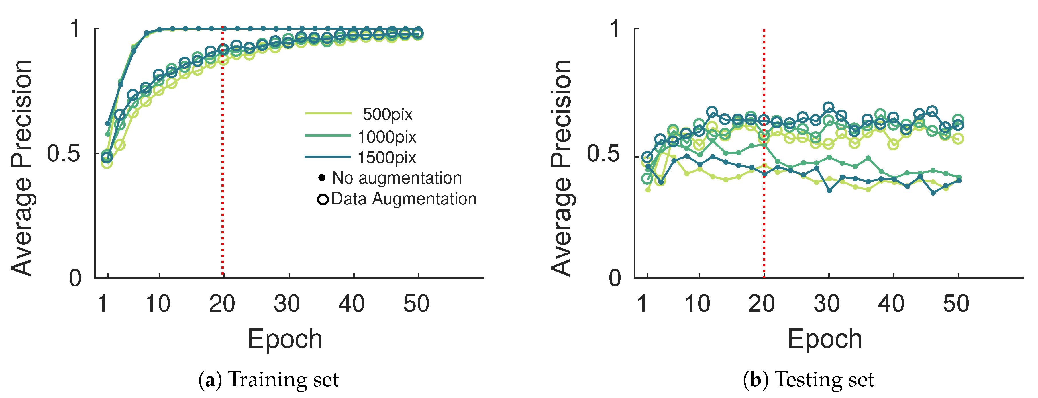
6. Conclusions and Perspectives

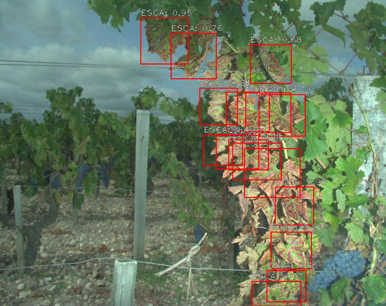
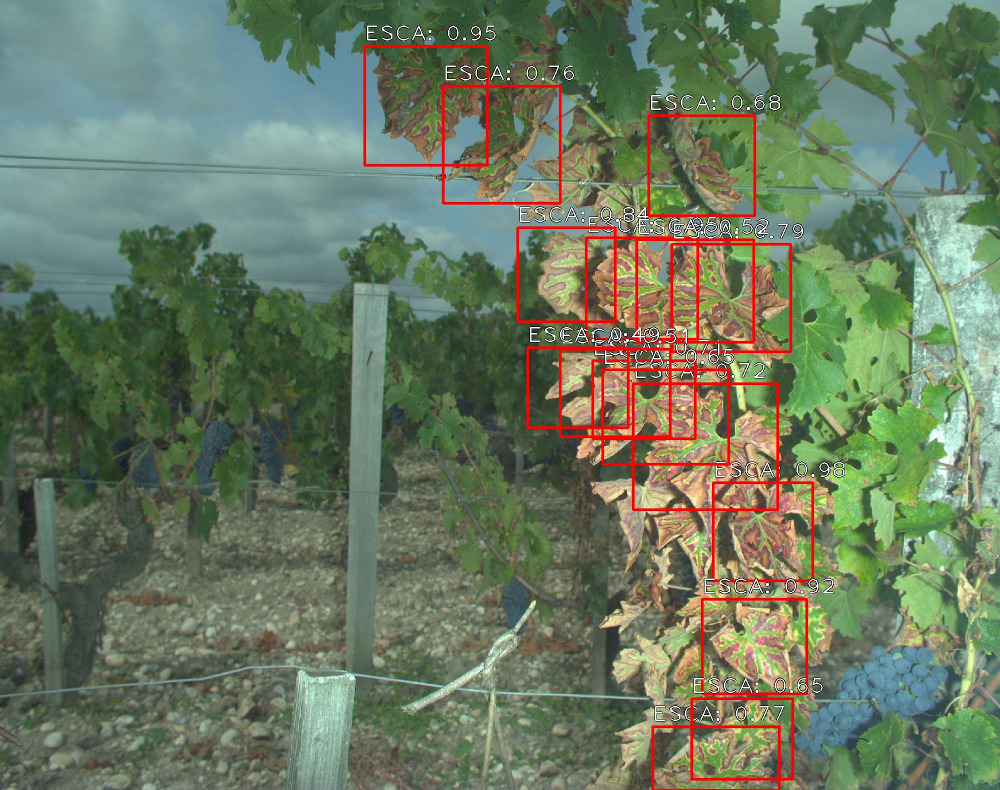
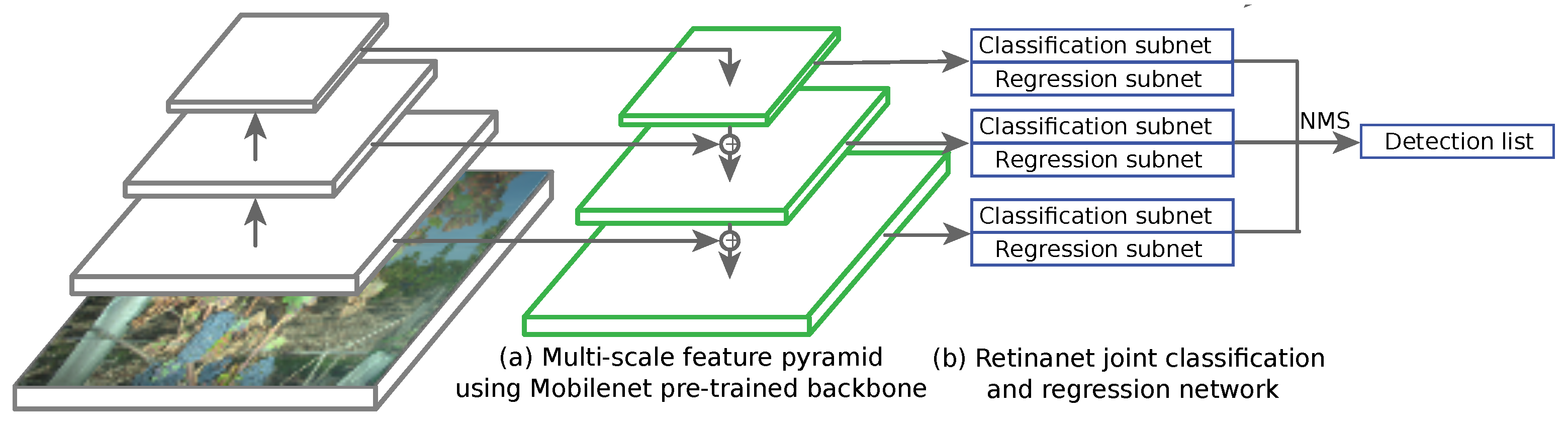
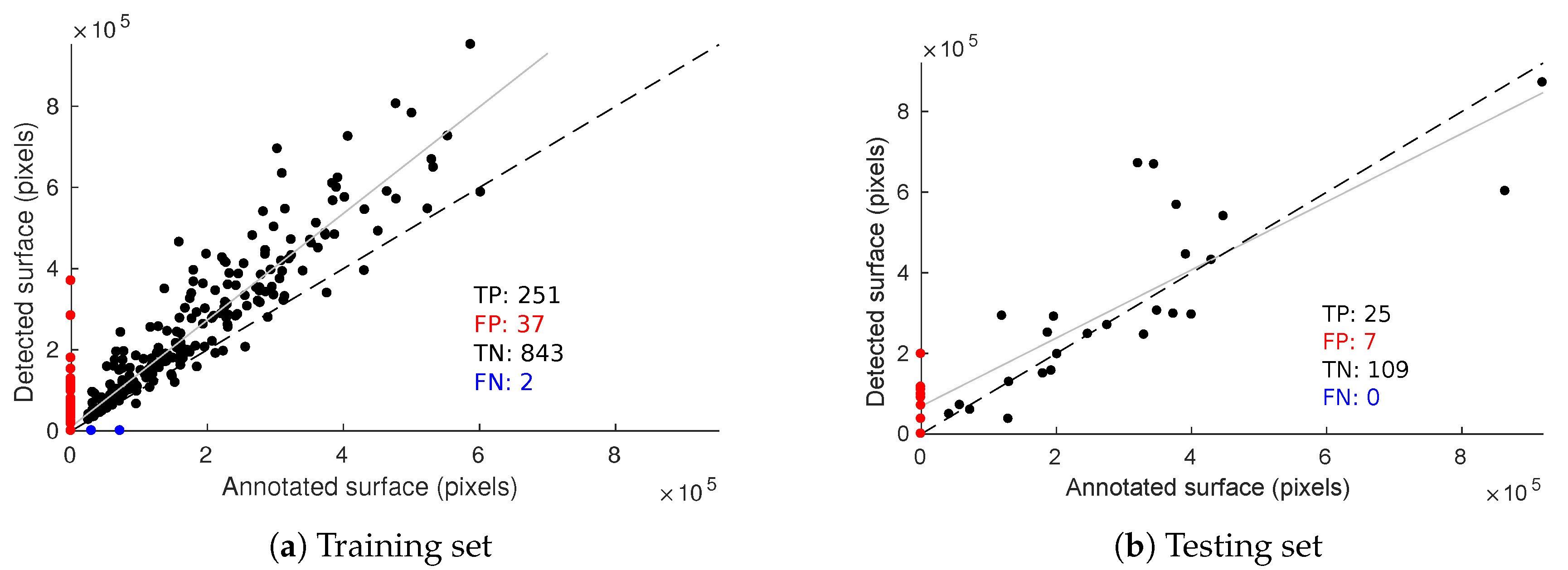
Plant diagnostic relies on the observation of the whole plant; it allows human observers to give, most of the time, accurate predictions about the plant status, although it is still error prone. In this paper, we propose a novel in-field esca symptom detector taking into account the differentiation with confounding factors. The first objective was to compare leaf-scale classification performances using state-of-the-art feature extractors. While SIFT based approaches using detected keypoints or grid of keypoints yielded good performances on challenging datasets, feature maps extracted from trained convolutional network (transfer learning) gave better results. Highest accuracy was thus achieved using deep mobilenet feature maps with global max pooling. In that case, spatial information allowed better discriminating esca from healthy leaves and other symptoms, especially for harder samples. While perfect classification on well-defined esca symptoms was easily achieved using these approaches, classification of less defined esca symptom remains a challenging task. The second objective was to exploit the discriminative power of the feature extractor to use it as the backbone in a detection algorithm at the plant scale. Based on the RetinaNet object segmentation model, the presented algorithm yields good results with an high correlation between the annotated esca surface and the detected surface for each plant. Furthermore, no esca annotated plant was missed during the prediction, meaning each symptomatic plant was correctly detected for a detection threshold of 0.5. Proximal sensing is thus a promising tool for precise disease detection, its rich spatial information can be used to discriminate between similar diseases in the vineyards, serving as a complementary tool to remote sensing surveys. Future works may include the construction of a broader in-field image database including more leaf symptoms and more grapevine cultivars, which is the next step for automatic and robust in-field grapevine disease detection.

References

1. Lecomte, P.; Darrieutort, G.; Liminana, J.M.; Comont, G.; Muruamendiaraz, A.; Legorburu, F.J.; Choueiri, E.; Jreijiri, F.; El Amil, R.; Fermaud, M. New Insights into Esca of Grapevine: The Development of Foliar Symptoms and Their Association with Xylem Discoloration. Plant Dis. 2012, 96, 924–934. [Google Scholar] [CrossRef]
2. Mugnai, L.; Graniti, A.; Surico, G. Esca (Black Measles) and Brown Wood-Streaking: Two Old and Elusive Diseases of Grapevines. Plant Dis. 1999, 83, 404–418. [Google Scholar] [CrossRef]
3. Larignon, P.; Darné, G.; Menard, E.; Desache, F.; Dudos, B. Comment agissait l’arsénite de sodium sur l’esca de la vigne ? Progrès Agricole et Viticole 2008, 125, 642–651. [Google Scholar]
4. Fussler, L.; Kobes, N.; Bertrand, F.; Maumy, M.; Grosman, J.; Savary, S. A Characterization of Grapevine Trunk Diseases in France from Data Generated by the National Grapevine Wood Diseases Survey. Ecol. Epidemiol. 2008, 98, 571–579. [Google Scholar] [CrossRef]
5. Barbedo, J.G.; Arnal Barbedo, J.G. Digital image processing techniques for detecting, quantifying and classifying plant diseases. SpringerPlus 2013, 2, 1–12. [Google Scholar] [CrossRef] [PubMed]
6. Mutka, A.M.; Bart, R.S. Image-based phenotyping of plant disease symptoms. Front. Plant Sci. 2015, 5, 734. [Google Scholar] [CrossRef] [PubMed]
7. Zheng, L.; Yang, Y.; Tian, Q. SIFT Meets CNN: A Decade Survey of Instance Retrieval. IEEE Trans. Pattern Anal. Mach. Intell. 2018, 40, 1224–1244. [Google Scholar] [CrossRef] [Green Version]
8. Oberti, R.; Marchi, M.; Tirelli, P.; Calcante, A.; Iriti, M.; Borghese, A.N. Automatic detection of powdery mildew on grapevine leaves by image analysis: Optimal view-angle range to increase the sensitivity. Comput. Electron. Agric. 2014, 104, 1–8. [Google Scholar] [CrossRef]
9. MacDonald, S.L.; Staid, M.; Staid, M.; Cooper, M.L. Remote hyperspectral imaging of grapevine leafroll-associated virus 3 in cabernet sauvignon vineyards. Comput. Electron. Agric. 2016, 130, 109–117. [Google Scholar] [CrossRef]
10. Fuentes, S.; De Bei, R.; Pech, J.; Tyermann, S. Computational water stress indices obtained from thermal image analysis of grapevine canopies. Irrig. Sci. 2012, 30, 523–536. [Google Scholar] [CrossRef]
11. Gaspero, G.D.; Bellin, D.; Ruperti, B. Pre-symptomatic detection of Plasmopara viticola infection in grapevine leaves using chlorophyll fluorescence imaging. Eur. J. Plant Pathol. 2009, 125, 291–302. [Google Scholar] [CrossRef]
12. Di Gennaro, S.F.; Battiston, E.; Di Marco, S.; Facini, O.; Matese, A. Unmanned Aerial Vehicle (UAV)-based remote sensing to monitor grapevine leaf stripe disease within a vineyard affected by esca complex. Phytopathol. Mediterr. 2009, 48, 159–188. [Google Scholar] [CrossRef]
13. Albetis, J.; Goulard, M. On the potentiality of UAV multispectral imagery to detect Flavescence dorée and Grapevine trunk. In Recent Advances in Quantitative Remote Sensing; Universidad de Valencia: València, Spain, 2017. [Google Scholar]
14. Al-saddik, H.; Laybros, A.; Billiot, B.; Cointault, F. Using Image Texture and Spectral Reflectance Analysis to Detect Yellowness and Esca in Grapevines at Leaf-Level. Remote Sens. 2018, 10, 618. [Google Scholar] [CrossRef]
15. Stewart, E.L.; Mcdonald, B.A. Measuring Quantitative Virulence in the Wheat Pathogen. Plant Pathol. 2014, 104, 985–992. [Google Scholar]
16. Wspanialy, P.; Moussa, M. Early powdery mildew detection system for application in greenhouse automation. Comput. Electron. Agric. 2016, 127, 487–494. [Google Scholar] [CrossRef]
17. Pang, J.; Bai, Z.Y.; Lai, J.C.; Li, S.K. Automatic Segmentation of Crop Leaf Spot Disease Images by Integrating Local Threshold and Seeded Region Growing. In Proceedings of the 2011 International Conference on Image Analysis and Signal Processing, Hubei, China, 21–23 October 2011; pp. 1–5. [Google Scholar]
18. Huang, K.Y. Application of artificial neural network for detecting Phalaenopsis seedling diseases using color and texture features. Comput. Electron. Agric. 2007, 57, 3–11. [Google Scholar] [CrossRef]
19. Lowe, D.G. Distinctive Image Features from Scale-Invariant Keypoints; Technical Report; University of British Columbia: Vancouver, BC, Canada, 2004. [Google Scholar]
20. Sivic, J.; Zisserman, A.; Kingdom, U. Video Google: A Text Retrieval Approach to Object Matching in Videos. In Proceedings of the Ninth IEEE International Conference on Computer Vision (ICCV’03), Nice, France, 13–16 October 2003. [Google Scholar]
21. Wilf, P.; Zhang, S.; Chikkerur, S.; Little, S.A.; Wing, S.L.; Serre, T. Computer vision cracks the leaf code. Proc. Natl. Acad. Sci. USA 2016, 113, 3305–3310. [Google Scholar] [CrossRef]
22. Kebapci, H.; Yanikoglu, B.; Unal, G. Plant image retrieval using color, shape and texture features. Comput. J. 2011, 54, 1475–1490. [Google Scholar] [CrossRef]
23. Quang_Khue, N.; Thi-Lan, L.; Ngoc-Hai, P. Leaf based plant identification system for Android using SURF features in combination with Bag of Words model and supervised learning. In Proceedings of the 2013 International Conference on Advanced Technologies for Communications (ATC 2013), Ho Chi Minh City, Vietnam, 16–18 October 2013; pp. 404–407. [Google Scholar]
24. Guo, W.; Fukatsu, T.; Ninomiya, S. Automated characterization of flowering dynamics in rice using field-acquired time-series RGB images. Plant Methods 2015, 11. [Google Scholar] [CrossRef]
25. Pires, R.D.L.; Goncalves, D.N.; Orue, J.P.M.; Kanashiro, W.E.S.; Rodrigues, J.F.; Machado, B.B.; Goncalves, W.N. Local descriptors for soybean disease recognition. Comput. Electron. Agric. 2016, 125, 48–55. [Google Scholar] [CrossRef]
26. Seeland, M.; Rzanny, M.; Alaqraa, N.; Wa, J. Plant species classification using flower images—A comparative study of local feature representations. PLoS ONE 2017. [Google Scholar] [CrossRef] [PubMed]
27. Shrivastava, S.; Singh, S.K.; Hooda, D.S. Soybean plant foliar disease detection using image retrieval approaches. Multimedia Tools Appl. 2017, 26647–26674. [Google Scholar] [CrossRef]
28. Prasad, S.; Kumar, P.; Hazra, R.; Kumar, A. Plant Leaf Disease Detection Using Gabor Wavelet Transform. In Proceedings of the International Conference on Swarm, Evolutionary and Memetic Computing, Visakhapatnam, India, 20–22 December 2012; pp. 372–379. [Google Scholar] [CrossRef]
29. Mohan, K.J.; Balasubramanian, M. Recognition of Paddy Plant Diseases Based on Histogram Oriented Gradient Features. Int. J. Adv. Res. Comput. Commun. Eng. 2016, 5, 3–6. [Google Scholar] [CrossRef]
30. Rosu, R.G.; Da Costa, J.P.; Donias, M. Structure tensor log-euclidean statistical models for texture analysis. In Proceedings of the International Conference on Image Processing, Phoenix, AZ, USA, 25–28 September 2016; pp. 2–6. [Google Scholar]
31. LeCun, Y.; Bottou, L.; Bengio, Y.; Haffner, P. Gradient based learning applied to document recognition. Process. IEEE 1998. [Google Scholar] [CrossRef]
32. Krizhevsky, A.; Sutskever, I.; Hinton, G.E. ImageNet Classification with Deep Convolutional Neural Networks. Adv. Neural Inf. Process. Syst. 2012, 1097–1105. [Google Scholar] [CrossRef]
33. Girshick, R.; Donahue, J.; Darrell, T.; Malik, J. Rich Feature Hierarchies for Accurate Object Detection and Semantic Segmentation; Technical Report; University of Berkeley, Department of Electrical Engineering and Computer Sciences: Berkeley, CA, USA, 2012. [Google Scholar]
34. Sun, Y.; Liu, Y.; Wang, G.; Zhang, H. Deep Learning for Plant Identification in Natural Environment. Comput. Intell. Neurosci. 2017, 2017. [Google Scholar] [CrossRef]
35. Ferentinos, K.P. Deep learning models for plant disease detection and diagnosis. Comput. Electron. Agric. 2018, 145, 311–318. [Google Scholar] [CrossRef]
36. Sladojevic, S.; Arsenovic, M.; Anderla, A.; Culibrk, D.; Stefanovic, D. Deep Neural Networks Based Recognition of Plant Diseases by Leaf Image Classification. Comput. Intell. Neurosci. 2016, 2016, 3289801. [Google Scholar] [CrossRef]
37. Fuentes, A.; Yoon, S.; Kim, S.C.; Park, D.S. A Robust Deep-Learning-Based Detector for Real-Time Tomato Plant Diseases and Pests Recognition. Sensors 2017, 17. [Google Scholar] [CrossRef]
38. Sa, I.; Ge, Z.; Dayoub, F.; Upcroft, B.; Perez, T.; McCool, C. Deepfruits: A fruit detection system using deep neural networks. Sensors 2016, 16. [Google Scholar] [CrossRef]
39. Tang, J.; Wang, D.; Zhang, Z.; He, L.; Xin, J.; Xu, Y. Weed identification based on K-means feature learning combined with convolutional neural network. Comput. Electron. Agric. 2017, 135, 63–70. [Google Scholar] [CrossRef]
40. Lu, H.; Cao, Z.; Xiao, Y.; Zhuang, B.; Shen, C. TasselNet: counting maize tassels in the wild via local counts regression network. Plant Methods 2017, 13, 79. [Google Scholar] [CrossRef]
41. Maaten, L.V.D.; Hinton, G. Visualizing Data using t-SNE. J. Mach. Learn. Res. 2008, 9, 2579–2605. [Google Scholar] [CrossRef]
42. Bosch, A.; Group, C.V.; Zisserman, A.; Group, C.V. Image Classification using Random Forests and Ferns. In Proceedings of the IEEE 11th International Conference on Computer Vision, Rio de Janeiro, Brazil, 14–21 October 2007. [Google Scholar]
43. Jégou, H.; Douze, M.; Schmid, C.; Pérez, P. Aggregating local descriptors into a compact image representation. In Proceedings of the IEEE Computer Society Conference on Computer Vision and Pattern Recognition, San Francisco, CA, USA, 13–18 June 2010; pp. 3304–3311. [Google Scholar] [CrossRef]
44. Perronnin, F.; Jorge, S.; Mensink, T. Improving the Fisher Kernel for Large-Scale Image Classification; Technical Report; Xerox Research Cenre Europe; Springer: Berlin, Germany, 2010. [Google Scholar]
45. Vedaldi, A.; Fulkerson, B. VLFeat—An open and portable library of computer vision algorithms. In Proceedings of the International Conference on Multimedia—MM ’10, Firenze, Italy, 25–29 October 2010; p. 1469. [Google Scholar] [CrossRef]
46. Howard, A.G.; Zhu, M.; Chen, B.; Kalenichenko, D.; Wang, W.; Weyand, T.; Andreetto, M.; Adam, H. MobileNets: Efficient Convolutional Neural Networks for Mobile Vision Applications; Technical Report; Google Inc.: Menlo Park, CA, USA, 2017. [Google Scholar]
47. Platt, J. Probabilistic outputs for support vector machines and comparisons to regularized likelihood methods. Adv. Large Margin Classif. 1999, 10, 61–74. [Google Scholar]
48. Mcnemar, Q. Note on the sampling error of the difference between correlated proportions or percentages. Psychometrika 1947, 12, 153–157. [Google Scholar] [CrossRef] [PubMed]
49. Lin, T.Y.; Goyal, P.; Girshick, R.; He, K.; Dollar, P. Focal Loss for Dense Object Detection. In Proceedings of the IEEE International Conference on Computer Vision, Venice, Italia, 22–29 October 2017; pp. 2999–3007. [Google Scholar] [CrossRef]
50. Lin, T.Y.; Girshick, R.; He, K.; Hariharan, B.; Belongie, S.; Tech, C. Feature Pyramid Networks for Object Detection; Technical Report; Facebook AI Reseach (FAIR); Cornell University and Cornell Tech: New York, NY, USA, 2016. [Google Scholar]
51. Kingma, D.P.; Ba, J.L. Adam: A method for stochastic optimization. In Proceedings of the International Conference on Learning Representations, San Diego, CA, USA, 7–9 May 2015; pp. 1–15. [Google Scholar]
Figure 1. (ad) Examples of well defined esca patterns; and (eh) examples of altered esca patterns.
Remotesensing 11 00001 g001
Figure 2. Examples of non-esca leaves showing foliar discolorations. (a) Black Rot, (b) Full yellowing, (c,d) Flavescence Dorée, (e) Wilted leaf, (f) Deficiency.
Remotesensing 11 00001 g002
Figure 3. (a) Detailed view of the sensor; and (b) sensor progressing through a vineyard row.
Remotesensing 11 00001 g003
Figure 4. Examples of pictures acquired in a vinerow.
Remotesensing 11 00001 g004
Figure 5. Schematic comparison of ideal (a) and real (b) class balance in esca leaf disease study. (c) Dimensionality reduction of feature maps extracted from the best performing approach in this paper (MobileNet off-the-shelf features from the 12th layer).
Remotesensing 11 00001 g005
Figure 6. (First row) (a) Keypoints map and (b) three examples of keypoints descriptors on a 4 × 4 grid on healthy leaf (extracted on hue channel); and (Second row) keypoints map and three examples of descriptors on esca leaf.
Remotesensing 11 00001 g006
Figure 7. Comparative description of SIFT encoding and CNN transfer learning for the construction of informative features.
Remotesensing 11 00001 g007
Figure 8. Overall accuracy on the white cultivar database as a function of the number of clusters/models used in the SIFT encoding part: (ac) the three types of encoding considered in the experiment. RGB fusion was used, concatenating each channel features into one final feature vector. Red Curve: DoG SIFT (keypoints); Light Green Curve: Dense SIFT (grid); Dark Green Curve: PHOW SIFT (multiscale grid); Dotted line: Best overall accuracy.
Remotesensing 11 00001 g008
Figure 9. White cultivar performances using features from pre-trained MobileNet 224 1.0 network for different depths using max pooling: (ac) performances for the three esca sublassses. Point size reflects dimensionality.
Remotesensing 11 00001 g009
Figure 10. Repartition of sorted SVM esca probabilities ([47]) in the test set. Green plots: asymptomatic leaves; light red to dark red plots: esca symptoms subclasses (from weak to strong); blue plots: other symptoms.
Remotesensing 11 00001 g010
Figure 11. One-step RetinaNet architecture in prediction mode, from full image input to detection list. The whole model is trained using a combination of classification loss and regression loss as the optimized objective function. MobileNet backbone’s convolutional layers were frozen so that only the parameters on the RetinaNet side evolve at a given epoch. Learning and weight updates are performed using standard backpropagation.
Remotesensing 11 00001 g011
Figure 12. Examples of detection maps using 1500 pixel images with data augmentation during training and 0.5 classification threshold. (a,c) Esca on red cultivar. (b,d) Esca on white cultivar.
Remotesensing 11 00001 g012
Figure 13. More segmentation examples: (a,b) confounding symptoms without esca false positives; (c,d) confounding symptoms with esca false positives; and (e,f) control plants with no esca false positives.
Remotesensing 11 00001 g013
Figure 14. Effect of the data augmentation parameter on training (a,b) and testing (c,d) esca RP curves. Epochs 1/10/20/30/40/50 are plotted. Dark green curves: early epochs; light green curves, late epochs. Vertical dotted lines in (c) indicate the maximum achieved recall.
Remotesensing 11 00001 g014
Figure 15. Evolution of the esca average precision metric on the training and testing set with the epoch during the training process.
Remotesensing 11 00001 g015
Figure 16. Relation between annotated and detected esca surface on the training (a) and testing (b) databases. Dotted line,: y = x reference; solid line, linear regression model on the true positives.
Remotesensing 11 00001 g016