Observing Water Vapour in the Planetary Boundary Layer from the Short-Wave Infrared


1
Earth Observation Science, Department of Physics & Astronomy, University of Leicester, University Road, Leicester LE1 7RH, UK
2
National Centre for Earth Observation, Department of Physics & Astronomy, University of Leicester, University Road, Leicester LE1 7RH, UK
3
Laboratoire de Météorologie Dynamique, Ecole Polytechnique–CNRS, 91128 Palaiseau, France
*
Author to whom correspondence should be addressed.
Remote Sens. 2018, 10(9), 1469; https://doi.org/10.3390/rs10091469
Submission received: 19 July 2018
/
Revised: 11 September 2018
/
Accepted: 11 September 2018
/
Published: 14 September 2018
(This article belongs to the Special Issue Remote Sensing Water Cycle: Theory, Sensors, Data, and Applications)
Abstract
:Water vapour is a key greenhouse gas in the Earth climate system. In this golden age of satellite remote sensing, global observations of water vapour fields are made from numerous instruments measuring in the ultraviolet/visible, through the infrared bands, to the microwave regions of the electromagnetic spectrum. While these observations provide a wealth of information on columnar, free-tropospheric and upper troposphere/lower stratosphere water vapour amounts, there is still an observational gap regarding resolved bulk planetary boundary layer (PBL) concentrations. In this study we demonstrate the ability of the Greenhouse Gases Observing SATellite (GOSAT) to bridge this gap from highly resolved measurements in the shortwave infrared (SWIR). These new measurements of near surface columnar water vapour are free of topographic artefacts and are interpreted as a proxy for bulk PBL water vapour. Validation (over land surfaces only) of this new data set against global radiosondes show low biases that vary seasonally between −2% to 5%. Analysis on broad latitudinal bands show biases between −3% and 2% moving from high latitudes to the equatorial regions. Finally, with the extension of the GOSAT program out to at least 2027, we discuss the potential for a new GOSAT PBL water vapour Climate Data Record (CDR).
1. Introduction
Water vapour is arguably the most important (non anthropogenic) greenhouse gas within the Earth climate system. Influencing (directly and indirectly) the radiative balance, surface fluxes and soil moisture, it is sufficiently abundant and short-lived that it is considered to be under natural control (Sherwood et al. [1]). With a prevalent positive feedback in the order of 2 W m−2 K−1 (Dessler et al. [2]), water vapour acts as the largest amplification mechanism for anthropogenic climate change compared to radiative forcing from greenhouse gases (Chung et al. [3]). This makes water vapour critical for climate studies (Held and Soden [4], Trenberth et al. [5]). The Planetary Boundary Layer (PBL) refers to the lowest region of the atmosphere (between 100 m to 3000 m) which is directly influenced by surface processes over both the land and ocean (Stull [6]). Containing approximately 80% of the total mass of atmospheric water vapour (Figure 1), the PBL regulates the exchange of heat, moisture, momentum, trace gases and aerosols between the Earths surface and the free troposphere (Myhre et al. [7]). The exchange of water vapour through evapotranspiration with the free troposphere is a key component in the water and energy cycle as without the subsequent phase changes most processes would be temperature driven (Stull [6]). Therefore accurate characterisation of heat and water vapour transport is needed to fully describe coupling between surface hydrology, clouds and precipitation (Prieto et al. [8]).
Long term satellite records of water vapour are dominated by observations from thermal infrared (TIR) and microwave (MW) sounders (Schröder et al. [9]). It is these data sets which are often used in climate analysis as well as being assimilated (at the radiance level) by numerical weather prediction (NWP) centres. However, from their nadir geometries these observations provide either estimates of the total column, or more recently coarse profiles of the troposphere. Measurements over land have a reduced sensitivity to lower-tropospheric water vapour as the apparent surface temperature, (function of surface emissivity and skin temperature) is close to the mean boundary layer temperature (Gao and Kaufman [10]), making it difficult to independently resolve the contribution from the near-surface. Further uncertainties are introduced by the large diurnal variability of skin temperatures and spectral emissivity over land (Prigent and Rossow [11]). Recent efforts have used data from the MODerate Resolution Imaging Spectroradiometer (MODIS) to infer information about boundary layer humidity. Feng et al. [12] sought to derive the boundary layer mixing height over the Heihe river basin in China, using air and dew-point temperature profiles from the MODIS MOD07 product (Seemann et al. [13]). While the profiles are supplied on 20 pressure levels the actual sensitivity of MODIS to water vapour vertical gradients is substantially lower, and will have a high dependence on the data set used to train the algorithm. The study by Millán et al. [14] also used MODIS to investigate water vapour in the marine boundary layer below low clouds. The authors used MODIS retrievals from the near-Infrared (NIR) above clouds (MYD05 L2 product) combined with coincident total column water vapour (TCWV) from the Advanced Microwave Scanning Radiometer (AMSR) aboard Aqua and GCOM-W1 platforms to derive partial column water vapour for the PBL. Estimates of TCWV from the NIR use the differential absorption technique (Gao et al. [15], Bartsch et al. [16], Albert et al. [17,18] to estimate atmospheric transmittances by comparing reflected solar radiation in water vapour absorption and nearby non-absorption/window channels (Gao and Kaufman [10]). By applying this method over fully cloudy scenes, estimates of columnar water vapour above the cloud can be made. These values are subtracted from TCWV estimates from AMSR to produce PBL partial column water vapour. While comparisons to radiosondes and ECMWF reanalysis showed robust results, the partial columns still showed differences from reference data sets of between 30% dry biased, to 26% wet biased.
This limitation is important as near-surface water vapour supplies the upper-atmosphere through vertical mixing (Willett et al. [19]). The study by Sherwood et al. [20] demonstrated that about half of the observed variance in climate sensitivity seen in models was associated with convective mixing between the lower and mid-troposphere. Current results suggest that global near surface air specific humidity has been increasing since the 1970s (Dai [21], Willett et al. [22]). However, recent in situ observations have shown a reduction in near surface moistening over land (Dai [21], Simmons et al. [23], Willett et al. [19]. This observed slowing in lower tropospheric moistening has resulted in an extensive decrease in near surface relative humidity in recent years (Myhre et al. [7]). Observations of near-surface/PBL water vapour over land are of interest as they provide information about the structure and diurnal evolution of the PBL. Such information can be instrumental in quantifying and improving land-atmosphere representations in coupled climate models; a weak link in our understanding of the Earth-Atmosphere system (Santanello et al. [24]). Therefore accurate observations of the water vapour in the PBL can help in developing our understanding of convective processes and regional responses to global warming.
While satellite observations traditionally used in NWP struggle to resolve the PBL, it has been demonstrated by Wagner et al. [25,26] and Noël et al. [27,28,29] that TCWV can also be successfully retrieved from visible (VIS) observations using instruments such as Global Ozone Monitoring Experiment (GOME), SCanning Imaging Absorption SpectroMeter for Atmospheric CHartographY (SCIAMACHY) or MEdium Resolution Imaging Spectrometer (MERIS). Such retrievals from VIS and shortwave infrared (SWIR) total column water vapour measurements are highly sensitive to near-surface air masses therefore providing the potential to overcome the limitations of MW and TIR instruments in observing PBL water vapour. An additional benefit of retrievals from the VIS and SWIR is that there is no dependence on skin temperature, and they only weakly depend on the atmospheric temperature profile.
Launched in late January 2009 by the Japanese space agency (JAXA), the Greenhouse Gases Observing SATellite (GOSAT) (Kuze et al. [30]) is the first dedicated greenhouse gas sensor suite. GOSAT observes nominally 5 cross track footprints with a diameter of 10.5 km which are separated by 100 km with a repeat cycle of 3 days. GOSAT carries two on-board instruments: (i) the Thermal And Near Infrared Sensor for carbon Observations Fourier Transform Spectrometer (TANSO-FTS) and (ii) the Cloud and Aerosol Imager (TANSO-CAI). The TANSO-FTS instrument covers four spectral bands with a high spectral resolution (0.3 cm−1). The first three operate in the NIR and SWIR centred around 0.76, 1.6 and 2.0 m with the fourth band operating in the TIR between 5.5 and 14.3 m. The Japanese National Institute for Environmental Studies (NIES) currently produces a column-averaged dry-air mole fraction water vapour () research product (Dupuy et al. [31], NIES [32]). Inter-comparisons of total column performed by Dupuy et al. [31] against measurements from the Total Carbon Column Observing Network (TCCON) showed a slight global dry bias in GOSAT (−3.10% ±24.00%). These results were attributed to altitude differences between the TCCON site and the GOSAT ground pixel and an artificial threshold within the product that causes dry biases in regions of high humidity. Further analysis of the GOSAT by Ohyama et al. [33] used coincident products from the GOSAT SWIR and TIR bands to assess the accuracy and variability of at TCCON sites. This study highlights the difficulty in validating GOSAT products due to the sparse global sampling. Their results showed an increase in variability from 6.70% to 18.50% by increasing the collocation window from 50 to 200 km.
In this study we show an approach to demonstrate the ability of GOSAT to resolve near surface columnar water vapour over land and sun-glint oceans. It is these partial columns that we use as a proxy for PBL water vapour, and from hereon in we refer to as PBL . In Section 2.1 we discuss our retrieval process for GOSAT water vapour from the SWIR and how we use the output to produce our estimates of PBL . Rather than using TCCON for our validation, we instead use radiosonde soundings from a harmonised global network. While temporal measurements are less frequent compared to TCCON, the larger number of stations allows us to accumulate a greater number of collocations which aids in the robustness of our validation approach. Results from these comparisons are shown in Section 3. Finally, we discuss the potential of GOSAT PBL water vapour as a potential future Essential Climate Variable (ECV).
2. Materials and Methods
2.1. The UoL Full Physics Retrieval Algorithm
The University of Leicester full physics retrieval (UoL-FP) algorithm (Cogan et al. [34]) was developed to retrieve XCO2 from a simultaneous fit of the near-infrared O2 A-Band spectrum at 0.76 m and the CO2 bands at 1.61 and 2.06 m as measured by NASA’s OCO-2 or the GOSAT instrument. The retrieval algorithm uses an iterative scheme based on Bayesian optimal estimation to retrieve a set of atmospheric/surface/instrument parameters, referred to as the state vector , from measured, calibrated spectral radiances. The forward model describes the physics of the measurement process and relates measured radiances to the state vector . It consists of a radiative transfer model (RTM) coupled to a model of the solar spectrum to calculate the spectrum of light that originates from the sun, passes through the atmosphere, reflects from the Earth’s surface or scatters back from the atmosphere, exits at the top of the atmosphere and enters the instrument. The top of atmosphere (TOA) radiances are then passed through the instrument model to simulate the measured radiances at the appropriate spectral resolution. The forward model employs the monochromatic scalar LIDORT (Spurr [35]) and TWOSTR (Spurr and Natraj [36]) radiative transfer models combined with a monochromatic, fast 2-orders-of-scattering vector radiative transfer code (Natraj and Spurr [37]). To accelerate the radiative transfer calculations for the entire spectral band, a method based on principal component analysis (PCA) has been utilised (Natraj et al. [38]). The specific implementation in the UoL algorithm makes use of a recent development which incorporates the spectrally varying aerosol scattering properties in an explicit manner (Somkuti et al. [39]). The TOA spectrum generated by the radiative transfer RT portion of the forward model is multiplied with a synthetic solar spectrum, which is calculated based on an empirical list of solar line parameters (Boesch et al. [40]). The instrument model then convolves the simulated radiance spectrum with an appropriate instrument line shape function (ILS) according to the specifications of the instrument.
Wrapped around the forward model is an inverse method which extracts information from the measurement. A detailed description of the inverse method can be found in Rodgers [41] and Connor et al. [42]. Briefly, the inverse method employs the Levenberg-Marquardt modification to the Gauss-Newton method to find the estimate of the state vector with the maximum a posteriori probability, given the measurement . The state vector typically includes profiles of the volume mixing ratio (VMR) of atmospheric absorbers, a temperature profile, aerosol and cloud extinction profiles, surface pressure, surface albedo and its spectral change for each band, as well as spectral dispersion shift and stretch for each band. Rather than retrieving full-profiles, the algorithm also allows for a profile scaling retrieval in which a single scaling factor for temperature or VMR profiles is determined. The algorithm can retrieve the aerosol extinction profiles for multiple aerosol and cloud types whose optical properties have been provided by the user. After the iterative retrieval process has converged to a solution, the posterior covariance matrix ,
and the averaging kernel matrix ,
are calculated with the a priori covariance matrix and the measurement error covariance matrix . is the Jacobian matrix, and represents the first-order derivative of the forward model with respect to the state vector elements, . The superscripts T and −1 are the specific matrix transpose and inverse respectively. The column-averaged dry air mole fraction of the target gas (here H2O) is inferred by averaging the retrieved H2O profile, weighted by the pressure weighting function (O’Dell et al. [43]), such that:
The associated column averaging kernel () is then given by:
with the variance of is calculated by applying the pressure weighting function to the posterior covariance matrix:
Thus, a retrieval approach very similar to the CO2 retrieval (O’Dell et al. [43], Connor et al. [42]) is adopted, where the O2 A band at 13,050 cm−1 (12,950.0–13,200.6 cm−1) and the strong CO2 band at 4850 cm−1 (4800.0–4902.2 cm−1) are jointly retrieved together with the H2O band at 5800 cm−1 (5814.0–5988.0 cm−1). These H2O windows chosen were based on regions with strong non-saturating, and weaker water vapour absorption lines. The main idea is to infer information on surface pressure, aerosols and clouds and temperature from the O2 band and the strong CO2 band, which bracket the H2O band—see Figure 2 for an example of the H2O and strong CO2 bands. We utilise the same spectroscopic data for O2, CO2, CH4 and H2O as described in Cogan et al. [34].
2.1.1. Estimating PBL Water Vapour
The UoL-FP setup for retrieving from GOSAT follows the description outlined in Boesch et al. [44]. Profiles of are retrieved on 20 pressure levels ranging between 1050 hPa to the TOA, with the lowest level being linearly interpolated in log space to the surface pressure. Therefore, in regions of high elevation effectively less than 20 levels are used. Within the UoL-FP processor additional state vector elements are also retrieved in addition to water vapour. These include:
- CO2 and temperature profile scaling factors,
- aerosol extinction profiles for two differing aerosol types and one cirrus type,
- surface pressure and surface albedo, and
- the spectral slope for each band.
The representation of these values in the initial state vector come from a number of sources. ECMWF is used to supply each sounding with the a priori values for surface pressure, temperature and water vapour profiles. For aerosol, global a priori values are described by Gaussian-shaped profiles for a height of 2 km, a width of 3 km and a total optical depth at 760 nm of 0.05. Differing optical properties taken from Kahn et al. [45] (aerosol mixtures 4b and 5b) and Baum et al. [46] (for effective radius of 60 m) are assigned to the aerosol a priori profiles. This strategy is employed to mitigate the effect of variable and unknown optical properties of the aerosols present for a given scene. For cirrus cloud the a priori profile is given by a latitude-, height- and width-dependent varying Gaussian profile with an optical depth of 0.05 (Eguchi et al. [47]). Retrieval of aerosol and cloud extinction are performed in log space to avoid negative values that would prevent the convergence of the retrieval. Finally, the CO2 a priori values are taken from a run of the LMDZ model (F. Chevallier, private communication), and the surface albedo a priori value is estimated for each band from the spectral ranges without significant absorption features.
The H2O a priori covariance matrix () has been generated using ECMWF water vapour profiles from June 2009. Northern-hemispheric mid-latitudinal profiles were used to calculate covariance and correlation matricies on the 20 level retrieval grid. A Markov process using five elements around the diagonal was then used to infer correlation-length. Next the stratosphere correlation lengths were set to zero and the covariance recalculated using the original diagonal elements, scaled by a factor of 20. This scaling results in having a total column water vapour variability of 22 kg/m2 (Figure 3). For the additional state vector elements the following a priori covariance matricies have been used:
- for aerosol and cirrus a diagonal matrix with an a priori 1 uncertainty of a factor of 10 for each level.
- temperature and CO2 scaling, the values 3.16 K and 0.316 ppm are used in the a priori covariance respectfully.
- a 1 value of 4 hPa is used for surface pressure, and
- surface albedo and its slope are essentially unconstrained.
The advantage of using both the 1.61- and 2.01-m bands is that more than two pieces of information can be retrieved for the column. This fact can then be used to separate out partial columns of based on the atmospheric regions resolved by integer values from the trace of the averaging kernel (). Starting from the surface, the Cumulative Degrees-Of-Freedom (CDOF) are calculated at each level in the profile. The closest level in the CDOF profile is set to one, the partial column top pressure (PCTP) is set as the highest altitude in the PBL layer. This information is then used to set the levels in the pressure weighting function above the PBL to zero. The updated pressure weighting function () is then applied to retrieved H2O profile so that:
where is the retrieved H2O profile and is the PBL partial column. The same approach could used to further sub-divide the column. For example, the free tropospheric partial column could be calculated for elements of the state vector which are bound between CDOF values of greater-or-equal than 1 and less-or-equal than 2. This concept is illustrated in Figure 4 and is also applied to the posterior covariance matrix to produce the retrieval uncertainty:
From here on the PBL subscript will be dropped as all quantities discussed are for the PBL only. Finally all VMR values are converted from ppm (part-per million) to specific humidity () units of g kg−1.
2.1.2. Uncertainties in GOSAT PBL Water Vapour
In this study we follow the approach taken in Connor et al. [42,48] by applying a linear analysis approach to assess uncertainties in retrieved PBL quantities. The a posterior uncertainty () is calculated as part of the retrieval output. This uncertainty will be an over-estimation as the a priori covariance matrix () used for H2O in the retrieval is relaxed to maximise the signal content coming from GOSAT. Therefore, a second value for the uncertainty in the retrieved PBL can also be calculated from the effects of the instrument noise, instrument smoothing of observed atmospheric state and the interference from the non-target state vector elements:
where is the updated retrieval uncertainty covariance matrix, is the measurement uncertainty covariance matrix, is the smoothing uncertainty covariance matrix, is the interference uncertainty covariance matrix (Rodgers [41]). The calculation of from the three uncertainty components is performed in post processing as and require the covariance of the ensemble of true states. The estimate the first term , we first calculate gain matrix ():
The gain matrix relates the sensitivity of the retrieved state vector to the measured radiance for a specific GOSAT scene. This property is then used to relate the random noise in the measured spectrum into state vector space:
where can be replaced for an alternative/updated estimate of measurement covariance if required. The uncertainty introduced by the constraint of the state vector on the a proiri is described by the smoothing uncertainty covariance matrix, and represents the smoothing of the true H2O profile on the retrieval:
where can be replaced for an alternative/updated estimate of measurement covariance if required. The uncertainty introduced by the constraint of the state vector on the a priori is described by the smoothing uncertainty covariance matrix and represents the smoothing of the true H2O profile on the retrieval:
where are the cross-talk elements of the averaging kernel that relate the response in the target elements to a -function perturbation in the non-target elements of the state vector (Rodgers [41]). Whilst being represented by a single term, is calculated for each non-target variable and summed together:
where is the non-target variable index. The corresponding variable and index number are shown in Table 1. The non-target uncertainties are described by an ensemble covariance matrix of the true state . The choice of which states to be included in are difficult to define, therefore we adopt the same approach used in Connor et al. [48] and use the a priori covariance . Further details on the non-target a priori covariances can be found in Cogan et al. [34].
Finally, the uncertainty covariances are used to calculate the retrieval uncertainty components such that:
which becomes:
where is the total retrieval uncertainty, is the measurement component of the retrieval uncertainty, is the smoothing component of the retrieval uncertainty and in the interference component of the retrieval uncertainty.
2.2. Assessment of PBL Water Vapour with Radiosondes
The performance of the GOSAT PBL is assessed against ground truth using the global radiosonde network. In this study we chose to use radiosondes rather than observations from water vapour Lidar networks (e.g., the international Network for the Detection of Atmospheric Composition Change (NDACC)) or aircraft measurements (e.g., In-service Aircraft for a Global Observing System (IAGOS)) due to the higher number of possible collocation sites. The motivation of this choice is primarily driven by significantly lower density of GOSAT sampling relative to its IR contemporaries such as AIRS and IASI. The large number of sites within the global radiosonde network allows for the required volume of collocations needed analyse GOSAT biases. This section describes the radiosonde data set used, the collocation and inter-comparison methodologies.
2.2.1. The Analyzed RadioSoundings Archive
Produced at the Laboratoire de Météorologie Dynamique (LMD) since the late 90’s, the Analyzed RadioSoundings Archive (ARSA) is designed for the processing and validation of level 1 (L1) and level 2 (L2) satellite data and for applications. This includes forward and inverse radiative transfer simulations, and inter-comparison of retrieved satellite geophysical parameters. The ARSA database is a global archive with observations from approximately 1450 stations (Figure 5). The vertical resolution of ARSA varies within the profile. The lowest part of the troposphere ranging from the surface to 800 hPa has a resolution of 0.50 km. Between 800 and 200 hPa the resolution is 0.80 km, increasing to 1.50 km from 200 hPa to 100 hPa. Above 100 hPa to the TOA the resolution reduces to 2.50 km. The measurement record starts in January 1979, and is regularly updated on a monthly basis. For this study we use the current version 2.7 archive, which has been in use since 2005.
The Processing of ARSA begins with the extraction of raw radiosonde measurements from the archive held at ECMWF. The multistage processor is then applied to each sounding to produce the end product:
- The first step is to apply physically coherent quality control tests to the raw radiosonde reports to (i) detect and eliminate gross errors, (ii) format problems, (iii) redundant radiosonde levels, (iv) unrealistic jumps, (v) physically implausible values, and (vi) temporal and vertical inconsistencies in temperature, dew point temperatures. Some of these tests benefit from the climatological Thermodynamic Initial Guess Retrieval (TIGR) data set (Chedin et al. [49], Chevallier et al. [50]).
- In the second step, quality control tests are applied to ensure that every radiosonde report kept after the first step is also fully compatible with the forward radiative transfer simulations. This requirement ensures discretization in pressure which is relevant to forward models. This is achieved by retaining profiles with (i) temperature measurements available at least up to 30 hPa, (ii) water vapour measurements available at pressure levels up to and above 350 hPa, and (iii) that the surface pressure be not smaller than 850 hPa over land and 950 hPa over sea.
- In the third step, whenever and wherever required information is missing, existing radiosonde measurements are combined with other reliable data sources in order to complete the description of the atmospheric state up to 0.0026 hPa. Temperature and water vapour profiles are extrapolated using ERA-Interim (Dee et al. [51]) outputs between 30 hPa and 0.1 hPa for temperature and between 300 hPa and 0.1 hPa for water vapour. Above 0.1 hPa, these same profiles are extrapolated up to 0.0026 hPa using a climatology of ACE/Scisat Level 2 (L2) products. In addition to temperature and water vapour, ozone profiles are also added to support forward model calculations. Since most of the radiosonde reports do not provide information on ozone, profiles from ERA Interim are spatially and temporally collocated with with the considered radiosonde station. When not available from the radiosonde report, surface temperature is taken from the surface station archive of ECMWF.
- For the fourth and final step, the temperature, water vapour, ozone profiles are interpolated onto a multi-level pressure grid between sea level pressure and 0.0026 hPa. This is nominally 43 pressure levels, however where necessary lower levels are removed to correspond with a radiosonde stations in altitude.
The precision of the ARSA profiles are the same as the original soundings on which they are based (below 300 hPa). The ARSA processor increases the accuracy of the measurement via statistical comparisons of simulated and observed TOA satellite radiances. The operational release of the Automatized Atmospheric Absorption Atlas radiative transfer model (4A/OP) is used as a transfer mechanism, which results in the improved radiance residuals relative to the original sounding or nominal reanalysis profile (Scott and Chedin et al. [52], Tournier et al. [53], Armante et al. [54]). The validation of ARSA, currently relies upon the study of statistics (bias, standard deviation) between simulated and observed satellite radiances e.g., from TOVS and ATOVS, as well as, in the more recent years, the Metop A&B IASI, HIRS4 and MHS observations. The simulated data are generated by the 4A/OP radiative transfer model, fed with the ARSA profile that is the closest (in space and time) from the satellite observation. This iterative, interactive validation process, uses thousands of land/sea/day/night globally collocated simulations-observations to: (i) identify spectral regions where an unexpected residual bias behaviour arises (ii) identify the spectral location and/or vertical pressure region source(s) of this bias; (iii) refine the statistics by tuning the atmospheric profile or surface characteristics. Further details and discussion are described in Scott [55] and Schröder et al. [9].
2.2.2. Collocation of GOSAT with ARSA
One of the challenges when validating any GOSAT product is collocating with enough in situ measurements in order to calculate meaningful statistics. For this study we adopt and adapt the criteria outlined in Trent et al. [56]. First a GOSAT footprint is considered collocated spatially if it is within 100 km of the ARSA launch site. The collocation distance () was calculated using the Haversine formula. Ideally the collocation distance between GOSAT and the radiosonde site would be less than 25 km (Calbet et al. [57]). However, the value of 100 km was used for collocation because the distance between GOSAT footprints across the swath ranges between 160-260 km depending on the GOSAT operating mode (Boesch et al. [44]).
Next a filter is applied to remove collocations that fall outside the time criteria. Calbet et al. [57] demonstrated that for (radiance) consistency between satellites and radiosondes, collocations need to be made within 30 min of the radiosonde launch. We adopt this same criterion in this study, removing all collocation outside 30 min either side of launch. By using a larger collocation distance than preferred allows for a greater number of collocations within the 30 minute overpass window. Next retrieval flags from the UoL-FP processor are applied to quality control GOSAT retrievals. In addition we also apply a surface pressure criteria. The retrieved GOSAT surface pressure is compared to the ARSA station surface pressure and collocations where the pressure difference is greater than 5 hPa are removed from the analysis set. This threshold is applied to avoid differences in air masses/altitude regimes being sampled by the radiosondes and satellite. The removal of this criteria has only a modest impact on the mean values of the fit. However, as a consequence more scatter, outliers and collocations that yield similar values for the wrong reason will be introduced. Finally, the collocated profiles are converted into ; Equation (6) is applied to the GOSAT retrieved H2O profile () and the ARSA profile is convert by applying the GOSAT column averaging kernel:
where is the ARSA water vapour profile, is the a priori profile and is the ARSA PBL water vapour. To look at the consistency between matches, one final statistical metric is calculated. This metric is taken from Immler et al. [58]:
where and are the satellite retrieved water vapour and retrieval uncertainty respectively, and and are the radiosonde measured water vapour and measurement uncertainty respectively and () is the collocation uncertainty. The variable describes the consistency of the comparison based on the assumption that , i.e., they have measured the same thing within uncertainty. For cases to be considered consistent would need to be less or equal to 1, less or equal to 2 and a case would be in (statistical) agreement. Values of of greater or equal to 3 are deemed inconsistent. The variables and are not known for this study, therefore rearranging Equation (17) in terms of becomes:
The values will not be used individually as a filter, rather by looking at how the mean values reduce on the scales of the analysis will provide insights to the robustness of our approach.
2.2.3. Testing the Suitability as a Proxy for PBL Water Vapour
The adaption of the UoL-FP algorithm in this study isolates the near surface partial column from the full column. With GOSAT’s high sensitivity to the near surface (Boesch et al. [44], Christi and Stephens [59], Kuang et al. [60]), the signal seen by GOSAT will be dominated by the PBL. Therefore, we have hypothesised that this near surface partial column acts as a proxy for PBL water vapour. To verify our hypothesis we compare PBL values calculated from the ARSA profiles using different values to represent the boundary layer height (BLH). These BLH values are used to update in Equation (6), while the ARSA profile replaces the state vector elements . Three BLH definitions are used:
- the PCTP, the lowest pressure level where the CDOF equal-or-less than 1,
- the Mixing Layer Height (MLH) calculated from the original ARSA radiosonde profile (MLH1),
- the MLH calculated from the ARSA radiosonde profile which has been linearly interpolated (in log H2O and log pressure space) on to the GOSAT retrieval pressure levels (MLH2).
When calculating the MLH from radiosonde profiles there are a number of approaches that can be implemented (Seidel et al. [61]). These are primarily based on either (i) the location of the maximum vertical gradient of potential temperature (Garratt et al. [62], Sorbjan [63], Stull [6]), (ii) the location of the minimum vertical gradient for either specific humidity, relative humidity or refractivity (Ao et al. [64], Sokolovskiy et al. [65], Basha and Ratnam [66]), (iii) elevated or surface based inversions (Bradley et al. [67]), (iv) the “parcel method” where the MLH is the pressure at which the virtual potential temperature of vertically displaced parcel of air is equal to the surface value (Holzworth [68], Seibert et al. [69]), and (v) bulk Richardson number threshold (Troen and Mahrt [70], Stull [6]). For this study we adopt and expand on the algorithm used in Boylan et al. [71]. For collocated GOSAT sounding with an ARSA profile we also calculate three additional PBL values based on the BLH definitions above. First a test is applied to the ARSA temperature profile to check whether the lapse rate gradient () at the surface is greater-or-equal to zero. If this test is true then the PBL is flagged as stable and the surface based inversion method is applied to calculate the MLH by identifying the top layer where is greater-or-equal to zero. If the lapse rate gradient is negative then the PBL is flagged as convective. The MLH is then identified by finding the minimum specific humidity vertical gradient location. Many studies use multiple methods to determine the BLH in convective conditions (e.g., Zang et al. [72]). This study only uses a single method as the coarse vertical resolution of the ARSA profiles and GOSAT retrieval grid are a greater source of uncertainty than the spread in the methodologies (Seidel et al. [61]). If MLH can be calculated from both versions of the ARSA profile (native and retrieval vertical resolutions), and the GOSAT collocation passes all the quality checks then the three PBL values are kept for later analysis.
3. Results
In this section we present the first results of PBL from GOSAT SWIR observations. Before these are discussed we first demonstrate that these new measurements can be considered a proxy PBL water vapour. The altitude at which the profile is integrated to in the retrieval process is based on the level at which the GOSAT resolves a single piece of information about the atmospheric state. By substituting this level for a MLH derived from the radiosonde profile it can be shown that these different values are representative of one another. Figure 6a shows the ARSA mean latitudinal PBL values for all three calculations PCTP, MLH1 and MLH2. All three cross sections show similar spatial distributions with the PCTP PBL yielding slightly higher values than the MLH PBL . These differences are represented as ratios in Figure 6b where largest values seen in the tropics at 5°N translates to a 23.90% and 28.15% over estimation in PBL for MLH1 and MLH2 methods respectively. In the tropics, the CDOF value for the PBL columns can be greater than 1. Using the inverse CDOF values as weights, the previous over-estimated ratios reduce to 4.60% and 11.26% respectively. This highlights the sensitivity of the PBL calculation to the coarse levels of the GOSAT retrieval grid. The larger disparity seen below 25 °N is partly influenced by the lower number of available soundings, which are ≈60% to 80% of those above 25 °N. Global mean ratios show that PCTP PBL values to be 13% and 9% higher than MLH1 and MLH2 PBL respectively. Another variable that contributes to the observed variability is the disparity between BLH values used in the PBL (Figure 6c). For negative differences where the MLH is higher in altitude than the PCTP, values generally result in ratios closer to 1. Positive differences where the PCTP is higher in altitude than the MLH result in the largest positive ratios.
3.1. GOSAT PBL Water Vapour Uncertainty Budget
To assess the breakdown of the GOSAT retrieval uncertainties we look at five representative cases for (i) Sahara desert, (ii) central Amazon rain forest, (iii) continental Europe, (iv) Greenland, and (v) sun-glint regions over the Pacific Ocean. For this analysis, retrievals have been taken from July 2017 with the individual measurements selected on the basis that they are the closest to the monthly mean values for the specific region being analysed. First we present the a posterior uncertainty, total retrieval uncertainty and it components (Equation (15)). These results are shown in Table 2.
Across all five regions the total retrieval uncertainty reduces from the a posterior uncertainty as expected. The most significant change seen for Greenland, where uncertainty on the retrieval shrinks by more than 50% of the original value. This is encouraging as the ice-covered surface of Greenland is a dark target in the SWIR, resulting in a much lower signal. This is evidenced by value for Greenland, which is nearly 10% of the measured PBL . Measurement and smoothing uncertainties are the dominant terms for all regions, with the interference uncertainties ranging between 0.5% and 1.5% of the PBL . This is encouraging as it shows that interfering species in the spectral windows used by the retrieval only have a small impact on the uncertainty. A key result from this analysis shows that it is possible to retrieve PBL over the Sahara, Amazon and ENSO region of the Pacific with uncertainties below 9%. This could be of use for future climate studies in these regions.
The second stage of the uncertainty budget breakdown is to look the impact of the non-target state element vector components on the retrieval uncertainty. Table 2 has already shown the total contribution of the interference uncertainty for the five sample regions. These singular values are in themselves the sum of their individual components (Equation (13)). The breakdown of the interference uncertainty budget into these individual elements is presented in Table 3. The key results from the decomposition of is that the scalar elements (CO2, CH4, Psurf and T) of the state vector have very little impact on the retrieval uncertainty, with no element contributing more than 0.4% of the total retrieval uncertainty. Aerosols and Cirrus are the greatest impact on , contributing between 86% to 97% of the total interference uncertainty budget. Albedo also has a very minimal impact both and .
3.2. Seasonal Distributions of GOSAT PBL Water Vapour
For a first look at GOSAT PBL water vapour we show seasonal maps (December 2016 to November 2017) of and the corresponding PCTP from both land and glint retrievals (Figure 7). The PCTP corresponds to the upper level (in pressure) of the retrieval pressure grid over which PBL is integrated. Seasonal variability of shows a distinct latitudinal gradients, with a ‘wet’ band following the Inter-Tropical Convergence Zone (ITCZ) that tails off to ‘drier’ values at higher latitudes. From visual inspection, monsoon activity is also visible over both Africa and India. With the northerly migration of the ITCZ across Africa, the intrusion of moist air into arid dessert/steppe regions can be seen in Figure 7a,c,e,g. Similarly, the same frames of Figure 7 show the increase in bulk PBL over India becoming ‘wetter’ as the seasons move from winter to summer. In the southern hemisphere, sensitivity to the Australian monsoon is also apparent. Finally, advection of along the warm sea surface temperatures of the Gulf stream into central Europe, with its subsidence in the Autumn also stands out.
The right-hand-side of Figure 7 shows the corresponding mean PCTP heights for seasonal estimates of . These plots demonstrate the topographic variability that could impact PBL column concentrations if reported as TCWV concentrations, a 1/g weighted integral of the specific humidity, where is the gravitational acceleration (9.806 ms−2). By using instead of TCWV the observation is of the column average rather than the sum of the whole column. This results in smaller gradient changes across varying topography. This is important because if a collocation occurs over a surface with a higher altitude than radiosonde launch point, then the resulting TCWV values could be considerably different. In this scenario a new source of bias would be introduced into the validation. From the PCTP maps the main geographic features that stand out are; (i) the Himalayas, (ii) the Rocky Mountains, (iii) the Andes, (iv) the Ethiopian Highlands, (v) the Kolyma Range and (vi) the Greenland ice-sheet. Interestingly, Figure 7e shows moister air either side of the Ural Mountains.
3.3. Comparisons at ARSA Ground Truth Sites
In this section we present results from inter-comparisons between GOSAT H2O retrievals (land only) and radiosonde ground truth sites. The collocation period used by this study spans between the 1 June 2009 and the 31 May 2017, from which more than 10,000 matches were collected for comparison. In contrast for the same period on 58 collocations were made for GOSAT sun-glint measurements using ARSA island stations. These results yielded a null hypothesis and as such have been omitted from the analysis. As the same reference source can not be used for both land ocean scenes we only focus on land results. For all comparisons presented here the outliers were first removed using the Bonferroni correction (Bonferroni [73], Dunn [74,75]).
To examine whether there is any seasonal dependence for GOSAT PBL biases, collocated cases were grouped into (Northern Hemisphere) winter (DJF), spring (MAM), summer (JJA) and the autumn (SON). Estimates of GOSAT biases relative to ARSA were estimated by robust Ordinary Least Squares (OLS) regression; the results of which are shown in Figure 8. The key points from the seasonal comparison are:
- GOSAT PBL biases range from 5.00 ± 0.01% in the winter to −2.00 ± 0.01% in the autumn, with an offset between 0.05 to 0.11 g kg−1.
- Seasonal mean squared error (MSE) values range from 0.05 to 0.08 g2 kg−2, which correspond to standard deviation values of 0.2 to 0.25 g kg−1.
- There is a large disparity between number of data points in each seasonal class. The highest number of collocations is found for summer months with 4373 cases, in stark contrast to winter months where there are only 975 cases found for the 8 year period.
- While there is a maximum spread of 0.25 g kg−1 in the seasonal results, correlation coefficients between GOSAT and ARSA PBL values are all greater than 0.9.
To further examine GOSAT biases, collocated cases were then split into three classes based on broad latitude bands. Collocations between 30°S and 30°N were grouped as tropical cases, the mid-latitude class included collocations between 45°S–30°S and 30°N–45°N, and finally everything above 45°N and below 45°S were grouped in the high-latitude class. Latitude bands were not split between northern and southern hemisphere bands as the difference in matches between the two hemispheres would not be comparable. Similar to the seasonal analysis, bias estimates are produced using OLS regression between GOSAT and ARSA (Figure 9). Restricting collocated cases to these three classes reduced bias estimates for GOSAT PBL relative to ARSA ground truth. Tropical cases show a small wet bias of 2.00 ± 0.01%, for mid-latitudes and high latitudes the OLS fit shows small dry biases of 1.00 ± 0.01% and 3.00 ± 0.01% respectively. While tropical results have a smaller wet bias than seasonal matches for DJF, MSE values are more than double (0.11 g2 kg−2). The mid-and-high latitudes cases, however, are comparable to seasonal results in MSE. Sampling at latitudes classified as being in the tropics show at least half the number of cases as those of the other two. Unlike seasonal comparisons, MSE does reduce with increasing collocation numbers. This can be attributed to the fact the spread in the data (1 ) significantly reduces at higher latitudes relative to the tropics (0.19 to 0.31 g kg−1 respectively). This indicates that spatial biases can be better characterised with additional suitable in situ measurements.
3.4. Consistency of Validation Approach
A key challenge in validating any L2 product from GOSAT is ensuring that collocated matches to ground truth are consistent within the total uncertainty of the match-up. This is especially true for water vapour as it varies on smaller temporal and spatial scales than other greenhouse gases such as CH4 or CO2. Due to the low frequency of GOSAT global observations relative to IR NWP sounders, it is therefore especially important to understand whether PBL bias estimates are in anyway weighted disproportionately. From Equation (17) we can see that terms for radiosonde and collocation/representation uncertainty are also included in the definition of stability. However, these values for this study are not available which will mean we consistently underestimate the full uncertainty budget. The ramification of this is that we will therefore consistently overestimate the magnitude . To mitigate this effect for this study we calculated seasonal values based on the whole eight year collocation period.
Figure 10 shows global distributions of GOSAT collocations at ARSA sites (Figure 10a,c,e,g) along with the corresponding consistency value (Figure 10b,d,f,h), on seasonal scales. Winter matches highlight the significant under-sampling relative to the other seasons. Results here are predominately clustered over North America, although comparisons on other continents show similar consistency performance. Higher collocation numbers in MAM, JJA and SON are concentrated between 30°N and 60° across North America and Europe. However, the rise in match-up density does not convert to an increase in performance in these areas. Mean values of range between 0.75 and 1.25 for the majority of collocation sites. Overall this performance level is representative of the majority of the global result, with a few areas where is greater than 2. These lower performing collocations are also in areas with very few, and in some cases only a single collocation for the whole 8 year period. In these scenarios it may be that the collocation criteria do not provide representative match-ups for the analysis.
4. Discussion
This study outlines a new approach for measuring bulk water vapour in the PBL using the water vapour absorption lines within 1.61 and 2.01 m SWIR bands of GOSAT. Through exploitation of the available DOF within the UoL full physics H2O retrievals, the near surface columnar water vapour content can be resolved. This partial column is heavily weighted by the near surface, which we have confirmed can act as a proxy for PBL water vapour under clear sky conditions (Figure 6). Traditionally, integrated volumes of atmospheric water vapour are expressed in units of kg m2, cm or mm. However, here we have used the column-averaged dry air mole fraction of the bulk PBL water vapour (denoted by the ‘X’) as it reduces the impact of topographic/surface pressure variability. This is of benefit because GOSAT significantly under-samples water vapour fields relative to IR NWP satellites. When aggregated to relatively coarse gridded monthly means, values would be disproportionately weighted by higher altitude surfaces when using TCWV. With the water vapour gradients are smaller than those of total column over varying altitude regimes.
This new GOSAT PBL data set has a number of strengths and weaknesses due to the primary focus of the mission being on observing changes in CO2 and CH4. The main weaknesses result from sampling as GOSAT is unable to capture day-to-day water vapour variability due to low frequency of observations within the swath. Operating within the SWIR region of the electromagnetic spectrum, GOSAT cannot sample any diurnal variation in PBL either. While this limitation restricts any changes on synoptic scales, inference can be drawn from monthly mean or seasonal PBL fields. With a local overpass time of around 13:00 hrs the vast majority of PBLs sampled by GOSAT are convective and as a result well-mixed. Therefore these measurements could act as boundary conditions for low cloud formation/feedback, which is a large source of uncertainty in climate models (Sherwood et al. [20]). Another strength of GOSAT is the accuracy to which it can measure water vapour in the PBL. From linear error analysis we have shown that PBL can be retrieved in key climate regions (e.g., the Sahara, Amazon and ENSO Pacific areas) with uncertainties below 9%. With the extension of the GOSAT series of instruments this is very encouraging for future climate studies. Over Greenland, the cold ice surface appears very dark in the SWIR. This results in a lower H2O signal and is a retrieval challenge. However, we demonstrate that GOSAT can measure the near surface over cold surfaces (polar summer only) with a 15.46% uncertainty. The selection of the spectroscopic windows have also been shown to have minor impact from non-target state vector elements, with the largest contribution from aerosols and clouds. The magnitude of the uncertainty contribution from these scatters is still less than 1% of PBL .
4.1. Global Distributions of PBL Water Vapour
The first global distribution of PBL are shown as seasonal maps (Figure 7). In all seasons clear varying latitudinal gradients can be seen, with no impact from large topographic features apparent in the corresponding PCTP fields. In addition to a clear seasonal cycle, GOSAT PBL also show sensitivity changes in water vapour fields due to advection and monsoon activity. This is very encouraging for future climate studies which will be made possible by future GOSAT missions which are currently scheduled to run until 2027 ([76]). Prior to February 2016, sun glint measurements are constricted to a band that oscillates between ±45° relative to hemispherical summer. The recent switch that now provides continuous sun glint measurements between and beyond ±45° will extend the potential climate analyses to ENSO based studies.
4.2. Validation at Global Radiosonde Sites
To better understand the performance of GOSAT PBL we have compared our retrievals with global radiosonde in situ measurements. For this validation task we have used the ARSA database produced by LMD as substantial care and effort has been applied to quality control and harmonise the archive. This study used atmospheric soundings from an eight year period (June 2009–May 2017) for the validation of GOSAT PBL . Once collocated ARSA profiles were convolved using the GOSAT column averaging kernel (Equation (16)) to ensure like-for-like comparisons. This match up database was first analysed by season (DJF, MAM, JJA & SON), where results showed biases below 5% (DJF) while getting as low as 1% for summer months. This result also revealed a imbalance in seasonal sampling, with winter months having only 22% of the number of collocations found in summer. Further examination of the collocations as a function of latitude show wet biases of 2% for tropical cases, while at mid-to-high latitudes are dry biased by 1% to 3% respectively. Again the disparity of match-ups is evident with tropical cases which make up only 17% of the total number of collocations. Unlike the seasonal analysis, MSE reduces with the increased number of collocations, from 0.11 g2 kg−2 to 0.04 g2 kg−2. This indicates that the collocation criteria are not always accounting for the variability of water vapour. Standard deviation values significantly reduce in the latitudinal analysis the further from the equator they are, while seasonally standard deviation values are more consistent. The differences in sampling arise as the majority of match-ups occur in the USA, Europe and Northern Asia (Figure 10). The lower solar elevation angles that occur during northern hemisphere winter restrict this area impacting the number of collocations. As the seasons progress into summer the collocation densities increase in the north, but in the southern hemisphere sees little change in collocation numbers. This, however is also the result of the lower number of radiosonde ground truth sites that can be used for validation, and presents a challenge when validating denser IR sounder measurements (Trent et al. [56]). To add confidence to the validation results, a consistency test based on Immler et al. [58] was calculated seasonally on a global 5° × 5° grid from the available collocations (Figure 10). This test normalises the difference between GOSAT and ARSA PBL by total uncertainty in the system. Without estimates of the uncertainty components from collocation and ARSA, only the GOSAT retrieval error is used. This underestimation in total uncertainty produces larger values, which could make some matches inconsistent and therefore non-comparable. We minimise this impact by averaging over the eight year collocation period. We are confident in this approach as the values for the majority of 5° × 5° grid cells reduces to below 0.75, i.e., ‘consistent’ with one-another. However, a number of regions have values ≥2 after averaging. While this is partly to do with low collocation number, future studies could use this information to filter stations which do not provide representative measurements on the spatial and temporal scales used to collocate with GOSAT. Identification of such sites, in addition to measurements that provide additional information for sun glint oceans or collocation uncertainty would be a focus of future PBL algorithm development. Overall GOSAT PBL H2O biases show a similar performance to AIRS Version 6 water vapour profile biases below 850 hPa (Trent et al. [56]) at global and climate radiosonde sites, which is very promising for climate studies.
5. Conclusions
In this study we have shown the first satellite single sensor estimates of bulk PBL water vapour over land and (sun glint) ocean. Due to the low spatial sampling of GOSAT only a small number of collocations were found for ocean scenes. This points to an existing limitation for many validation studies. Future work would need to look at trying to increase the number of reference measurements for sun-glint retrievals as well as southern hemisphere land sites which are also disproportionately under-sampled during collocation. Guidance could be taken the Gap Analysis for Integrated Atmospheric ECV CLImate Monitoring (GAIA-CLIM) project (http://www.gaia-clim.eu/) which has addressed these types of issues in detail. Through the adaption of the existing UoL GOSAT full physics algorithm, we have established the ability to resolve near surface columnar water vapour amounts that serve as useful proxy for PBL . The majority of current satellite water vapour records provide estimates of TCWV only (e.g., Schröder et al. [77]), with modern hyper-spectral IR sounders now producing coarsely resolved tropospheric water vapour profiles. The new measurements from GOSAT compliment these existing records and add to our understanding of water vapour variability in the troposphere. These records will be further enhanced with the launch of GOSAT-2, which unlike GOSAT will operate intelligent pointing to avoid cloudy scenes and thus increase global coverage (Glumb et al. [78]). Validation efforts from this study further demonstrate low biases from GOSAT PBL estimates. Coupled with the potential longevity of the GOSAT program, which includes GOSAT-2 (2018) and GOSAT-3 (2022) platforms (WMO [76]), these low biased measurements could allow GOSAT to provide the first satellite Climate Data Record (CDR) of PBL water vapour. This record would compliment existing climate records from the Hadley Centre and Climate Research Unit (HadISDH) (Willett et al. [19], Smith et al. [79]) and the Hamburg Ocean Atmosphere Parameters and Fluxes from Satellite data (HOAPS) (Anderson et al. [80]), which provide global near surface humidity measurements (). GOSAT PBL will provide a bridge between , TCWV and (potentially) water vapour profiles, extending our knowledge of tropospheric water vapour in the Earth climate system.
Author Contributions
Conceptualization, T.T. and H.B.; Data curation, T.T., P.S. and N.A.S.; Formal analysis, T.T.; Investigation, T.T., H.B. and P.S.; Methodology, T.T., H.B. and P.S.; Resources, H.B., P.S. and N.A.S.; Software, T.T., H.B., P.S. and N.A.S.; Supervision, H.B.; Validation, T.T. and N.A.S.; Visualization, T.T.; Writing—original draft, T.T., H.B., P.S. and N.A.S.; Writing—review & editing, T.T., H.B., P.S. and N.A.S.
Funding
Tim Trent, Peter Somkuti & Hartmut Boesch would like to acknowledge the funding from Natural Environment Research Council (NERC) through Natural Centre for Earth Observation (NCEO), contract number PR140015. Noëlle A. Scott acknowledges the ongoing support from the Centre National d’Etudes Spatiales (CNES).
Acknowledgments
The authors would like to thank the Japanese Aerospace Exploration Agency, National Institute for Environmental Studies, and the Ministry of Environment for the GOSAT data and their continuous support as part of the Joint Research Agreement. The GOSAT L1B data are available from the GOSAT data archive service (GDAS, https://data2.gosat.nies.go.jp/index_en.html). ECMWF ERA-Interim data are available through the ECMWF website (http://apps.ecmwf.int/datasets/). Noëlle A. Scott also acknowledges the ECMWF Data Server for making available the ERA-interim outputs, the radiosonde archive and the surface station archive that enter the composition of the ARSA database. The authors would like to acknowledge the Atmospheric Radiation Analysis (ARA)/Atmosphère-Biosphère-Climat (télédétection) (ABC(t))/LMD group for producing and making available the Analyzed RadioSounding Archive (ARSA) database (http://ara.abct.lmd.polytechnique.fr/index.php?page=arsa). This research used the ALICE/SPECTRE High Performance Computing Facility at the University of Leicester, as well as the NERC JASMIN data processing environment at the Centre for Environmental Analysis (CEDA).
Conflicts of Interest
The authors declare no conflict of interest.
Abbreviations
The following abbreviations are used in this manuscript:
| AMSR | Advanced Microwave Scanning Radiometer |
| ARSA | Analyzed RadioSoundings Archive |
| ATOVS | Advanced TIROSOperational Vertical Sounder |
| BLH | Boundary Layer Height |
| CAI | Cloud and Aerosol Imager |
| CDR | Climate Data Record |
| CDOF | Cumulative Degrees-of-Freedom |
| ECMWF | European Centre for Medium-Range Weather Forecast |
| ECV | Essential Climate Variable |
| ERA-Interim | ECMWF Reanalysis Interim |
| GAIA-CLIM | Gap Analysis for Integrated Atmospheric ECV CLImate Monitoring |
| GOME | Global Ozone Monitoring Experiment |
| GOSAT | Greenhouse Gases Observing SATellite |
| HadISDH | Met Office Hadley Centre led project utilising ISD Humidity data |
| HIRS | High-resolution Infra Red Sounder |
| HOAPS | The Hamburg Ocean Atmosphere Parameters and Fluxes from Satellite Data |
| IAGOS | In-service Aircraft for a Global Observing System |
| IASI | Infrared Atmospheric Sounding Interferometer |
| ILS | Instrument Lineshape function |
| ITCZ | Inter Tropical Convergence Zone |
| JAXA | Japanese space agency |
| L1 | Level 1 (data product) |
| L2 | Level 2 (data product) |
| LIDORT | Linearized Discrete Ordinate Radiative Transfer |
| LMDZ | Laboratoire de Météorologie Dynamique Zoom |
| MERIS | MEdium Resolution Imaging Spectrometer |
| MHS | Microwave Humididty Sounder |
| MLH | Mixing Layer Height |
| MODIS | Moderate Resolution Imaging Spectroradiomete |
| MSE | Mean Squared Error |
| MW | Microwave |
| NDACC | Network for the Detection of Atmospheric Composition Change |
| NIES | National Institute for Environmental Studies |
| NIR | Near Infrared |
| NWP | Numerical Weather Prediction |
| OCO-2 | Orbiting Carbon Observatory 2 |
| OLS | Ordinary Least Squares |
| PBL | Planetary Boundary Layer |
| PCA | Priciple Component Analysis |
| PCTP | Partial Column Top Pressure |
| q2m | 2 metre surface specific humidity |
| SCIAMACHY | SCanning Imaging Absorption SpectroMeter for Atmospheric CHartographY |
| SWIR | Short Wave Infrared |
| TANSO-FTS | Thermal And Near Infrared Sensor for carbon Observations Fourier Transform Spectrometer |
| TCCON | Total Carbon Column Observing Network |
| TCWV | Total Column Water Vapour |
| TIGR | Thermodynamic Initial Guess Retrieval |
| TIR | Thermal Infrared |
| TIROS | Television and Infrared Operational Satellite |
| TOA | Top-of-Atmosphere |
| TOVS | TIROS Operational Vertical Sounder |
| UoL-FP | University of Leicester full physics retrieval |
| VIS | Visible |
| VMR | Volume Mixing Ratio |
References
- Sherwood, S.; Roca, R.; Weckwerth, T.; Andronova, N. Tropospheric water vapor, convection, and climate. Rev. Geophys. 2010, 48. [Google Scholar] [CrossRef] [Green Version]
- Dessler, A.; Zhang, Z.; Yang, P. Water-vapor climate feedback inferred from climate fluctuations, 2003–2008. Geophys. Res. Lett. 2008, 35. [Google Scholar] [CrossRef] [Green Version]
- Chung, E.S.; Soden, B.; Sohn, B.; Shi, L. Upper-tropospheric moistening in response to anthropogenic warming. Proc. Natl. Acad. Sci. USA 2014, 111, 11636–11641. [Google Scholar] [CrossRef] [PubMed] [Green Version]
- Held, I.M.; Soden, B.J. Water vapor feedback and global warming. Annu. Rev. Energy Environ. 2000, 25, 441–475. [Google Scholar] [CrossRef]
- Trenberth, K.E.; Fasullo, J.; Smith, L. Trends and variability in column-integrated atmospheric water vapor. Clim. Dyn. 2005, 24, 741–758. [Google Scholar] [CrossRef]
- Stull, R.B. An Introduction to Boundary Layer Meteorology; Springer Science & Business Media: Berlin, Germany, 2012; Volume 13. [Google Scholar]
- Myhre, G.; Shindell, D.; Bréon, F.; Collins, W.; Fuglestvedt, J.; Huang, J.; Koch, D.; Lamarque, J.; Lee, D.; Mendoza, B.; et al. Climate Change 2013: The Physical Science Basis. Contribution of Working Group I to the Fifth Assessment Report of the Intergovernmental Panel on Climate Change; Tignor, M., Allen, S.K., Boschung, J., Nauels, A., Xia, Y., Bex, V., Midgley, P.M., Eds.; Cambridge University Press: Cambridge, UK; New York, NY, USA, 2013. [Google Scholar]
- Prieto, D.; van Oevelen, P.; Rast, M.; Senevirantne, S.; Stephens, G. ESA-GEWEX earth observation and water cycle science priorities. In Proceedings of the ‘Earth Observation for Water Cycle Science’, Frascati, Italy, 23–26 October 2015. [Google Scholar]
- Schröder, M.; Lockhoff, M.; Shi, L.; August, T.; Bennartz, R.; Borbas, E.; Brogniez, H.; Calbet, X.; Crewell, S.; Eikenberg, S.; et al. GEWEX Water Vapor Assessment (G-VAP); WCRP Report 16/2017; World Climate Research Programme (WCRP): Geneva, Switzerland, 2017; p. 216. [Google Scholar]
- Gao, B.C.; Kaufman, Y.J. Water vapor retrievals using Moderate Resolution Imaging Spectroradiometer (MODIS) near-infrared channels. J. Geophys. Res. Atmos. 2003, 108. [Google Scholar] [CrossRef] [Green Version]
- Prigent, C.; Rossow, W. Retrieval of surface and atmospheric parameters over land from SSM/I: Potential and limitations. Q. J. R. Meteorol. Soc. 1999, 125, 2379–2400. [Google Scholar] [CrossRef]
- Feng, X.; Wu, B.; Yan, N. A method for deriving the boundary layer mixing height from modis atmospheric profile data. Atmosphere 2015, 6, 1346–1361. [Google Scholar] [CrossRef]
- Seemann, S.W.; Li, J.; Menzel, W.P.; Gumley, L.E. Operational retrieval of atmospheric temperature, moisture, and ozone from MODIS infrared radiances. J. Appl. Meteorol. 2003, 42, 1072–1091. [Google Scholar] [CrossRef]
- Millán, L.; Lebsock, M.; Fishbein, E.; Kalmus, P.; Teixeira, J. Quantifying marine boundary layer water vapor beneath low clouds with near-infrared and microwave imagery. J. Appl. Meteorol. Climatol. 2016, 55, 213–225. [Google Scholar] [CrossRef]
- Gao, B.; Goetz, A.; Westwater, E.R.; Conel, J.; Green, R. Possible near-IR channels for remote sensing precipitable water vapor from geostationary satellite platforms. J. Appl. Meteorol. 1993, 32, 1791–1801. [Google Scholar] [CrossRef]
- Bartsch, B.; Bakan, S.; Fischer, J. Passive remote sensing of the atmospheric water vapour content above land surfaces. Adv. Space Res. 1996, 18, 25–28. [Google Scholar] [CrossRef]
- Albert, P.; Bennartz, R.; Fischer, J. Remote sensing of atmospheric water vapor from backscattered sunlight in cloudy atmospheres. J. Atmos. Ocean. Technol. 2001, 18, 865–874. [Google Scholar] [CrossRef]
- Albert, P.; Bennartz, R.; Preusker, R.; Leinweber, R.; Fischer, J. Remote sensing of atmospheric water vapor using the moderate resolution imaging spectroradiometer. J. Atmos. Ocean. Technol. 2005, 22, 309–314. [Google Scholar] [CrossRef]
- Willette, K.M.; Williams, C.N., Jr.; Dunn, R.J.; Thorne, P.; Bell, S.; de Podesta, M.; Jones, D.; Parker, D.E. HadISDH land surface multi-variable humidity and temperature record for climate monitoring. Clim. Past 2014, 10, 1983–2006. [Google Scholar] [CrossRef]
- Sherwood, S.C.; Bony, S.; Dufresne, J.L. Spread in model climate sensitivity traced to atmospheric convective mixing. Nature 2014, 505, 37–42. [Google Scholar] [CrossRef] [PubMed]
- Dai, A. Recent climatology, variability, and trends in global surface humidity. J. Clim. 2006, 19, 3589–3606. [Google Scholar] [CrossRef]
- Willett, K.M.; Jones, P.D.; Gillett, N.P.; Thorne, P.W. Recent changes in surface humidity: Development of the HadCRUH dataset. J. Clim. 2008, 21, 5364–5383. [Google Scholar] [CrossRef]
- Simmons, A.; Willett, K.; Jones, P.; Thorne, P.; Dee, D. Low-frequency variations in surface atmospheric humidity, temperature, and precipitation: Inferences from reanalyses and monthly gridded observational data sets. J. Geophys. Res. Atmos. 2010, 115. [Google Scholar] [CrossRef] [Green Version]
- Santanello, J.A., Jr.; Friedl, M.A.; Kustas, W.P. An empirical investigation of convective planetary boundary layer evolution and its relationship with the land surface. J. Appl. Meteorol. 2005, 44, 917–932. [Google Scholar] [CrossRef]
- Wagner, T.; Heland, J.; Zöger, M.; Platt, U. A fast H2O total column density product from GOME—Validation with in-situ aircraft measurements. Atmos. Chem. Phys. 2003, 3, 651–663. [Google Scholar] [CrossRef]
- Wagner, T.; Beirle, S.; Grzegorski, M.; Platt, U. Global trends (1996–2003) of total column precipitable water observed by Global Ozone Monitoring Experiment (GOME) on ERS-2 and their relation to near-surface temperature. J. Geophys. Res. Atmos. 2006, 111. [Google Scholar] [CrossRef] [Green Version]
- Noël, S.; Buchwitz, M.; Bovensmann, H.; Hoogen, R.; Burrows, J.P. Atmospheric water vapor amounts retrieved from GOME satellite data. Geophys. Res. Lett. 1999, 26, 1841–1844. [Google Scholar] [CrossRef] [Green Version]
- Noël, S.; Buchwitz, M.; Bovensmann, H.; Burrows, J. Validation of SCIAMACHY AMC-DOAS water vapour columns. Atmos. Chem. Phys. 2005, 5, 1835–1841. [Google Scholar] [CrossRef] [Green Version]
- Noël, S.; Mieruch, S.; Bovensmann, H.; Burrows, J. Preliminary results of GOME-2 water vapour retrievals and first applications in polar regions. Atmos. Chem. Phys. 2008, 8, 1519–1529. [Google Scholar] [CrossRef] [Green Version]
- Kuze, A.; Suto, H.; Nakajima, M.; Hamazaki, T. Thermal and near infrared sensor for carbon observation Fourier-transform spectrometer on the Greenhouse Gases Observing Satellite for greenhouse gases monitoring. Appl. Opt. 2009, 48, 6716–6733. [Google Scholar] [CrossRef] [PubMed]
- Dupuy, E.; Morino, I.; Deutscher, N.M.; Yoshida, Y.; Uchino, O.; Connor, B.J.; De Mazière, M.; Griffith, D.W.; Hase, F.; Heikkinen, P.; et al. Comparison of XH2O retrieved from GOSAT short-wavelength infrared spectra with observations from the TCCON network. Remote Sens. 2016, 8, 414. [Google Scholar] [CrossRef]
- NIES. NIES GOSAT TANSO-FTS SWIR Level 2 Data Product Format Description; National Institute for Environmental Studies GOSAT Project; NIES-GOSAT-PO-006-21; National Institute for Environmental Studies: Tsukuba, Japan, 2017. [Google Scholar]
- Ohyama, H.; Kawakami, S.; Shiomi, K.; Morino, I.; Uchino, O. Intercomparison of XH2O Data from the GOSAT TANSO-FTS (TIR and SWIR) and Ground-Based FTS Measurements: Impact of the Spatial Variability of XH2O on the Intercomparison. Remote Sens. 2017, 9, 64. [Google Scholar] [CrossRef]
- Cogan, A.; Boesch, H.; Parker, R.; Feng, L.; Palmer, P.; Blavier, J.F.; Deutscher, N.M.; Macatangay, R.; Notholt, J.; Roehl, C.; et al. Atmospheric carbon dioxide retrieved from the Greenhouse gases Observing SATellite (GOSAT): Comparison with ground-based TCCON observations and GEOS-Chem model calculations. J. Geophys. Res. Atmos. 2012, 117. [Google Scholar] [CrossRef] [Green Version]
- Spurr, R. LIDORT and VLIDORT: Linearized pseudo-spherical scalar and vector discrete ordinate radiative transfer models for use in remote sensing retrieval problems. In Light Scattering Reviews 3; Springer: Berlin, Germany, 2008; pp. 229–275. [Google Scholar]
- Spurr, R.; Natraj, V. A linearized two-stream radiative transfer code for fast approximation of multiple-scatter fields. J. Quant. Spectrosc. Radiat. Transf. 2011, 112, 2630–2637. [Google Scholar] [CrossRef]
- Natraj, V.; Spurr, R.J. A fast linearized pseudo-spherical two orders of scattering model to account for polarization in vertically inhomogeneous scattering–absorbing media. J. Quant. Spectrosc. Radiat. Transf. 2007, 107, 263–293. [Google Scholar] [CrossRef]
- Natraj, V.; Jiang, X.; Shia, R.l.; Huang, X.; Margolis, J.S.; Yung, Y.L. Application of principal component analysis to high spectral resolution radiative transfer: A case study of the O2 A band. J. Quant. Spectrosc. Radiat. Transf. 2005, 95, 539–556. [Google Scholar] [CrossRef]
- Somkuti, P.; Boesch, H.; Natraj, V.; Kopparla, P. Application of a PCA-Based Fast Radiative Transfer Model to XCO2 Retrievals in the Shortwave Infrared. J. Geophys. Res. Atmos. 2017, 122, 10477–10496. [Google Scholar] [CrossRef]
- Boesch, H.; Toon, G.; Sen, B.; Washenfelder, R.; Wennberg, P.; Buchwitz, M.; de Beek, R.; Burrows, J.; Crisp, D.; Christi, M.; et al. Spacebased Near-Infrared CO2 Retrievals: Testing the OCO Retrieval and Validation Concept Using SCIAMACHY Measurements over Park Falls, Wisconsin. J. Geophys. Res 2006, 111, D23302. [Google Scholar]
- Rodgers, C.D. Inverse Methods for Atmospheric Sounding: Theory and Practice; World Scientific: Singapore, 2000; Volume 2. [Google Scholar]
- Connor, B.J.; Boesch, H.; Toon, G.; Sen, B.; Miller, C.; Crisp, D. Orbiting Carbon Observatory: Inverse method and prospective error analysis. J. Geophys. Res. Atmos. 2008, 113. [Google Scholar] [CrossRef] [Green Version]
- O’Dell, C.W.; Connor, B.; Bösch, H.; O’Brien, D.; Frankenberg, C.; Castano, R.; Christi, M.; Eldering, D.; Fisher, B.; Gunson, M.; et al. The ACOS CO2 retrieval algorithm—Part 1: Description and validation against synthetic observations. Atmos. Meas. Tech. 2012, 5, 99–121. [Google Scholar] [CrossRef]
- Boesch, H.; Baker, D.; Connor, B.; Crisp, D.; Miller, C. Global characterization of CO2 column retrievals from shortwave-infrared satellite observations of the Orbiting Carbon Observatory-2 mission. Remote Sens. 2011, 3, 270–304. [Google Scholar] [CrossRef]
- Kahn, R.; Banerjee, P.; McDonald, D. Sensitivity of multiangle imaging to natural mixtures of aerosols over ocean. J. Geophys. Res. Atmos. 2001, 106, 18219–18238. [Google Scholar] [CrossRef] [Green Version]
- Baum, B.A.; Heymsfield, A.J.; Yang, P.; Bedka, S.T. Bulk scattering properties for the remote sensing of ice clouds. Part I: Microphysical data and models. J. Appl. Meteorol. 2005, 44, 1885–1895. [Google Scholar] [CrossRef]
- Eguchi, N.; Yokota, T.; Inoue, G. Characteristics of cirrus clouds from ICESat/GLAS observations. Geophys. Res. Lett. 2007, 34. [Google Scholar] [CrossRef] [Green Version]
- Connor, B.; Bösch, H.; McDuffie, J.; Taylor, T.; Fu, D.; Frankenberg, C.; O’Dell, C.; Payne, V.H.; Gunson, M.; Pollock, R.; et al. Quantification of uncertainties in OCO-2 measurements of XCO2: Simulations and linear error analysis. Atmos. Meas. Tech. 2016, 9, 5227–5238. [Google Scholar] [CrossRef]
- Chedin, A.; Scott, N.; Wahiche, C.; Moulinier, P. The improved initialization inversion method: A high resolution physical method for temperature retrievals from satellites of the TIROS-N series. J. Clim. Appl. Meteorol. 1985, 24, 128–143. [Google Scholar] [CrossRef]
- Chevallier, F.; Chéruy, F.; Scott, N.; Chédin, A. A neural network approach for a fast and accurate computation of a longwave radiative budget. J. Appl. Meteorol. 1998, 37, 1385–1397. [Google Scholar] [CrossRef]
- Dee, D.P.; Uppala, S.; Simmons, A.; Berrisford, P.; Poli, P.; Kobayashi, S.; Andrae, U.; Balmaseda, M.; Balsamo, G.; Bauer, D.P.; et al. The ERA-Interim reanalysis: Configuration and performance of the data assimilation system. Q. J. R. Meteorol. Soc. 2011, 137, 553–597. [Google Scholar] [CrossRef]
- Scott, N.; Chedin, A. A fast line-by-line method for atmospheric absorption computations: The Automatized Atmospheric Absorption Atlas. J. Appl. Meteorol. 1981, 20, 802–812. [Google Scholar] [CrossRef]
- Tournier, B.; Armante, R.; Scott, N. STRANSAC-93 et 4A-93: Developpement et Validation des Nouvelles Versions des Codes de Transfert Radiatif Pour Application au Projet IASI; Internal Rep. LMD; Ecole Polytechnique: Palaiseau, France, 1995. [Google Scholar]
- Armante, R.; Scott, N.; Crevoisier, C.; Capelle, V.; Crepeau, L.; Jacquinet, N.; Chédin, A. Evaluation of spectroscopic databases through radiative transfer simulations compared to observations. Application to the validation of GEISA 2015 with IASI and TCCON. J. Mol. Spectrosc. 2016, 327, 180–192. [Google Scholar] [CrossRef] [Green Version]
- Scott, N. Quality Assessment of Satellite and Radiosonde Data; EUMETSAT CM SAF Visiting Scientist Report; Satellite Application Facility on Climate Monitoring (CM SAF): Offenbach, Germany, 2015. [Google Scholar]
- Trent, T.; Schröder, M.; Remedios, J. GEWEX Water Vapor Assessment: Validation of AIRS Tropospheric Humidity Profiles with Characterised Radiosonde Soundings. J. Geophys. Res. Atmos. 2018. under review. [Google Scholar]
- Calbet, X.; Peinado-Galan, N.; Rípodas, P.; Trent, T.; Dirksen, R.; Sommer, M. Consistency between GRUAN sondes, LBLRTM and IASI. Atmos. Meas. Tech. 2017, 10, 2323. [Google Scholar] [CrossRef]
- Immler, F.; Dykema, J.; Gardiner, T.; Whiteman, D.; Thorne, P.; Vömel, H. Reference quality upper-air measurements: Guidance for developing GRUAN data products. Atmos. Meas. Tech. 2010, 3, 1217–1231. [Google Scholar] [CrossRef]
- Christi, M.; Stephens, G. Retrieving profiles of atmospheric CO2 in clear sky and in the presence of thin cloud using spectroscopy from the near and thermal infrared: A preliminary case study. J. Geophys. Res. Atmos. 2004, 109. [Google Scholar] [CrossRef]
- Kuang, Z.; Margolis, J.; Toon, G.; Crisp, D.; Yung, Y. Spaceborne measurements of atmospheric CO2 by high-resolution NIR spectrometry of reflected sunlight: An introductory study. Geophys. Res. Lett. 2002, 29, 11-1–11-4. [Google Scholar] [CrossRef]
- Seidel, D.J.; Ao, C.O.; Li, K. Estimating climatological planetary boundary layer heights from radiosonde observations: Comparison of methods and uncertainty analysis. J. Geophys. Res. Atmos. 2010, 115. [Google Scholar] [CrossRef] [Green Version]
- Garratt, J. The Atmospheric Boundary Layer; Cambridge Atmospheric and Space Science Series; Cambridge University Press: Cambridge, UK, 1992; Volume 416, p. 444. [Google Scholar]
- Sorbjan, Z. Structure of the Atmospheric Boundary Layer; Number 551.51 SOR; Prentice Hall: Upper Saddle River, NJ, USA, 1989. [Google Scholar]
- Ao, C.; Chan, T.; Iijima, B.; Li, J.; Mannucci, A.; Teixeira, J.; Tian, B.; Waliser, D. Planetary boundary layer information from GPS radio occultation measurements. In Proceedings of the GRAS SAF Workshop on Applications of GPSRO Measurements, Reading, UK, 16–18 June 2008; pp. 123–131. [Google Scholar]
- Sokolovskiy, S.; Kuo, Y.H.; Rocken, C.; Schreiner, W.; Hunt, D.; Anthes, R. Monitoring the atmospheric boundary layer by GPS radio occultation signals recorded in the open-loop mode. Geophys. Res. Lett. 2006, 33. [Google Scholar] [CrossRef] [Green Version]
- Basha, G.; Ratnam, M.V. Identification of atmospheric boundary layer height over a tropical station using high-resolution radiosonde refractivity profiles: Comparison with GPS radio occultation measurements. J. Geophys. Res. Atmos. 2009, 114. [Google Scholar] [CrossRef] [Green Version]
- Bradley, R.S.; Keimig, F.T.; Diaz, H.F. Recent changes in the North American Arctic boundary layer in winter. J. Geophys. Res. Atmos. 1993, 98, 8851–8858. [Google Scholar] [CrossRef]
- Holzworth, G.C. Estimates of mean maximum mixing depths in the contiguous United States. Mon. Weather Rev. 1964, 92, 235–242. [Google Scholar] [CrossRef]
- Seibert, P.; Beyrich, F.; Gryning, S.E.; Joffre, S.; Rasmussen, A.; Tercier, P. Review and intercomparison of operational methods for the determination of the mixing height. Atmos. Environ. 2000, 34, 1001–1027. [Google Scholar] [CrossRef]
- Troen, I.; Mahrt, L. A simple model of the atmospheric boundary layer; sensitivity to surface evaporation. Bound.-Layer Meteorol. 1986, 37, 129–148. [Google Scholar] [CrossRef] [Green Version]
- Boylan, P.; Wang, J.; Cohn, S.A.; Fetzer, E.; Maddy, E.S.; Wong, S. Validation of AIRS version 6 temperature profiles and surface-based inversions over Antarctica using Concordiasi dropsonde data. J. Geophys. Res. Atmos. 2015, 120, 992–1007. [Google Scholar] [CrossRef] [Green Version]
- Zang, Z.; Wang, W.; Cheng, X.; Yang, B.; Pan, X.; You, W. Effects of Boundary Layer Height on the Model of Ground-Level PM2. 5 Concentrations from AOD: Comparison of Stable and Convective Boundary Layer Heights from Different Methods. Atmosphere 2017, 8, 104. [Google Scholar] [CrossRef]
- Bonferroni, C. Teoria statistica delle classi e calcolo delle probabilita. Pubblicazioni del R Istituto Superiore di Scienze Economiche e Commericiali di Firenze 1936, 8, 3–62. [Google Scholar]
- Dunn, O.J. Estimation of the Means of Dependent Variables. Ann. Math. Stat. 1958, 29, 1095–1111. [Google Scholar] [CrossRef]
- Dunn, O.J. Multiple Comparisons Among Means. J. Am. Stat. Assoc. 1961, 56, 52–64. [Google Scholar] [CrossRef]
- WMO OSCAR Satellite Programme: Greenhouse Gas Observing Satellite. Available online: https://www.wmo-sat.info/oscar/satelliteprogrammes/view/66 (accessed on 2 July 2018).
- Schröder, M.; Lockhoff, M.; Fell, F.; Forsythe, J.; Trent, T.; Bennartz, R.; Borbas, E.; Bosilovich, M.G.; Castelli, E.; Hersbach, H.; et al. The GEWEX Water Vapor Assessment archive of water vapour products from satellite observations and reanalyses. Earth Syst. Sci. Data 2018, 10, 1093. [Google Scholar] [CrossRef]
- Glumb, R.; Davis, G.; Lietzke, C. The tanso-fts-2 instrument for the gosat-2 greenhouse gas monitoring mission. In Proceedings of the 2014 IEEE International Geoscience and Remote Sensing Symposium (IGARSS), Quebec City, QC, Canada, 13–18 July 2014; IEEE: Piscataway, NJ, USA, 2014; pp. 1238–1240. [Google Scholar]
- Smith, A.; Lott, N.; Vose, R. The integrated surface database: Recent developments and partnerships. Bull. Am. Meteorol. Soc. 2011, 92, 704–708. [Google Scholar] [CrossRef]
- Andersson, A.; Graw, K.; Schröder, M.; Fennig, K.; Liman, J.; Bakan, S.; Hollmann, R.; Klepp, C. Hamburg Ocean Atmosphere Parameters and Fluxes from Satellite Data—HOAPS 4.0; Satellite Application Facility on Climate Monitoring: Hessen, Germany, 2017. [Google Scholar] [CrossRef]
Figure 1.
Ratio of PBL to total column (TC) concentrations calculated using profiles from the Analyzed Radio Soundings Archive (ARSA), which is described in Section 2.2.1. Ratios are shown as a function latitude, year and season, where DJF (December, January, February) is northern hemisphere (NH) winter, MAM (March, April, May) is NH spring, JJA (June, July, August) is NH summer, and SON (September, October, November) is NH autumn. Latitudinal cross sections are shown for each year of the study with the overall ratio mean () and standard deviation () for all years shown in the sub-headings.

Figure 2.
Example GOSAT short wave infrared spectra for bands 2 (a) and 3 (b). Contribution of main absorbers for bands 2 and 3 are shown in (c,d) respectively. Spectral lines of absorbers are shown at the native resolution of the spectrascopic database and have not had the GOSAT instrument line shape applied.
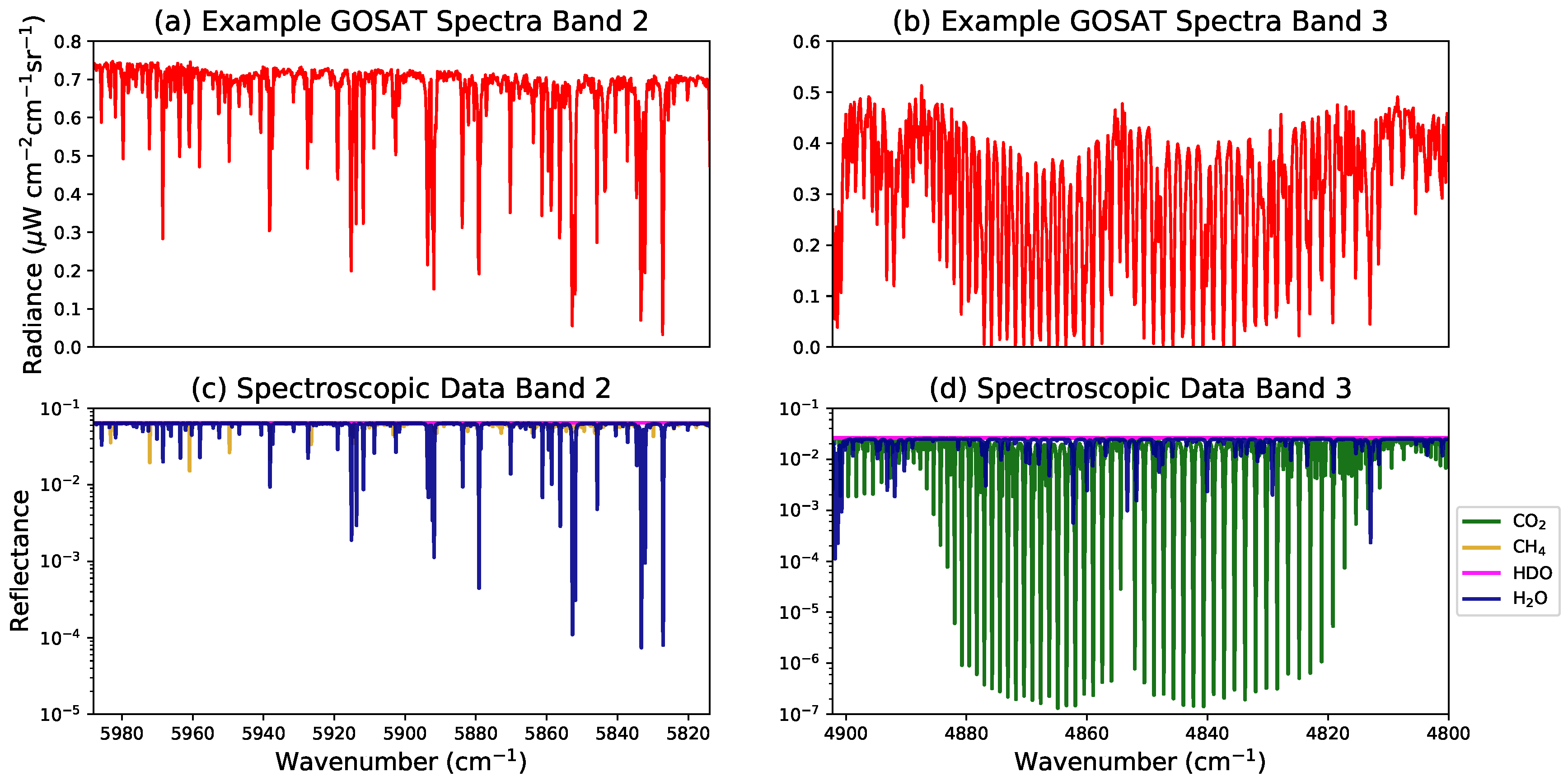
Figure 3.
Water vapour prior covariance matrix (a) with the corresponding correlation matrix (b). The effect of zero correlation length in stratospheric levels can be seen in panel (b), were they are represented by grey regions.
Figure 3.
Water vapour prior covariance matrix (a) with the corresponding correlation matrix (b). The effect of zero correlation length in stratospheric levels can be seen in panel (b), were they are represented by grey regions.

Figure 4.
Example of how GOSAT full averaging kernel (AK) is transformed into partial column averaging kernels by exploiting the degrees of freedom in the XH2O retrieval. An example of the full averaging kernel is shown in panel (a) with each level colour-coded. The application of the pressure weighting function to the full averaging kernel is shown in panel (b). The column averaging kernel is shown as a dashed black line, while the partial column averaging kernels based on the cumulative degrees-of-freedom (CDOF) being equal to 0–1, 1–2 and greater than 2 are represented by the blue, green and red lines respectively.
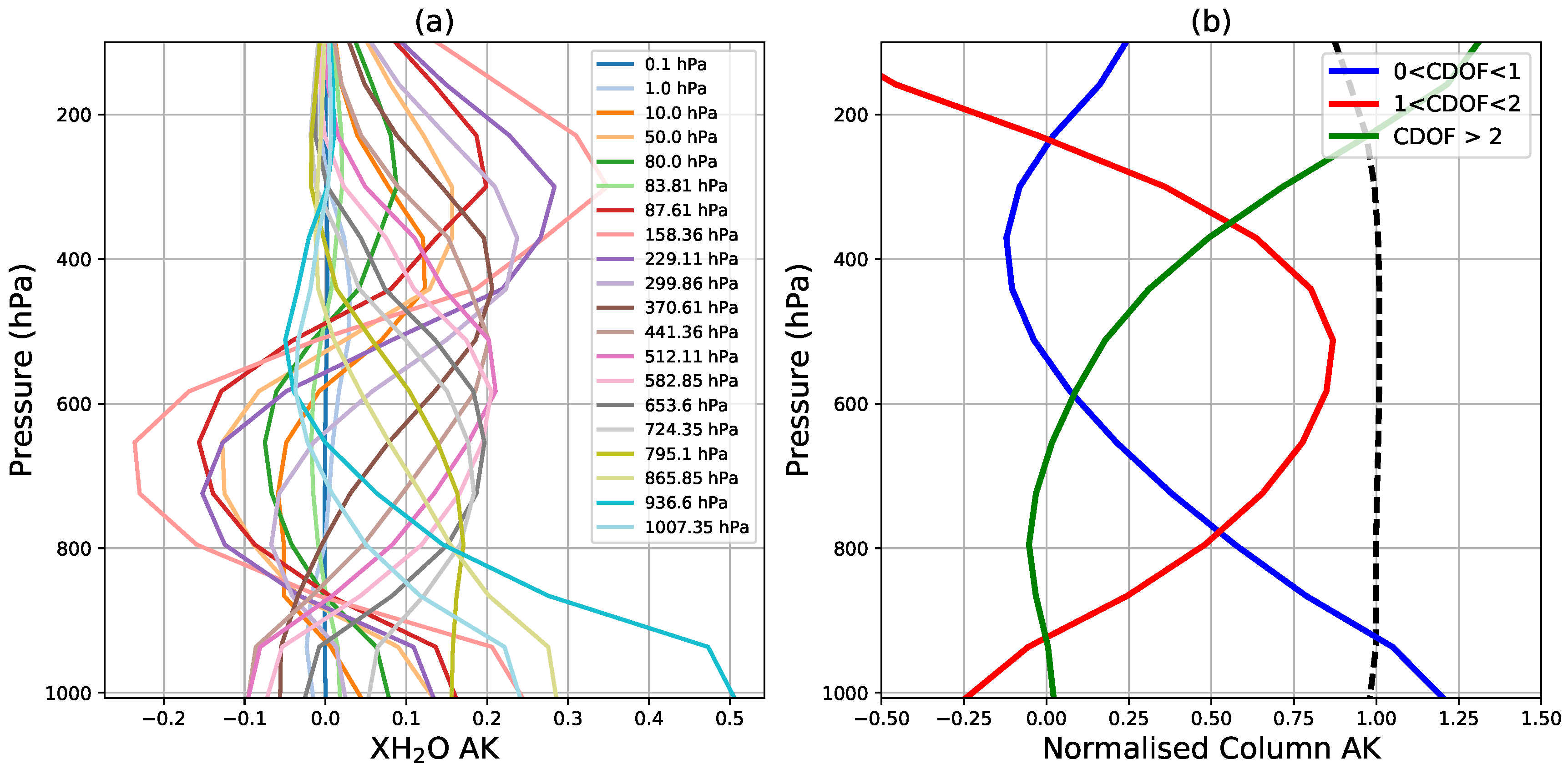
Figure 5.
Global distribution of ARSA radiosonde stations between January 2009–December 2017. These locations were used to first extract GOSAT overpasses that fell within the collocation criteria. In total 1,744,215 ARSA profiles are available from 582 sites within the 8 year analysis period.
Figure 5.
Global distribution of ARSA radiosonde stations between January 2009–December 2017. These locations were used to first extract GOSAT overpasses that fell within the collocation criteria. In total 1,744,215 ARSA profiles are available from 582 sites within the 8 year analysis period.
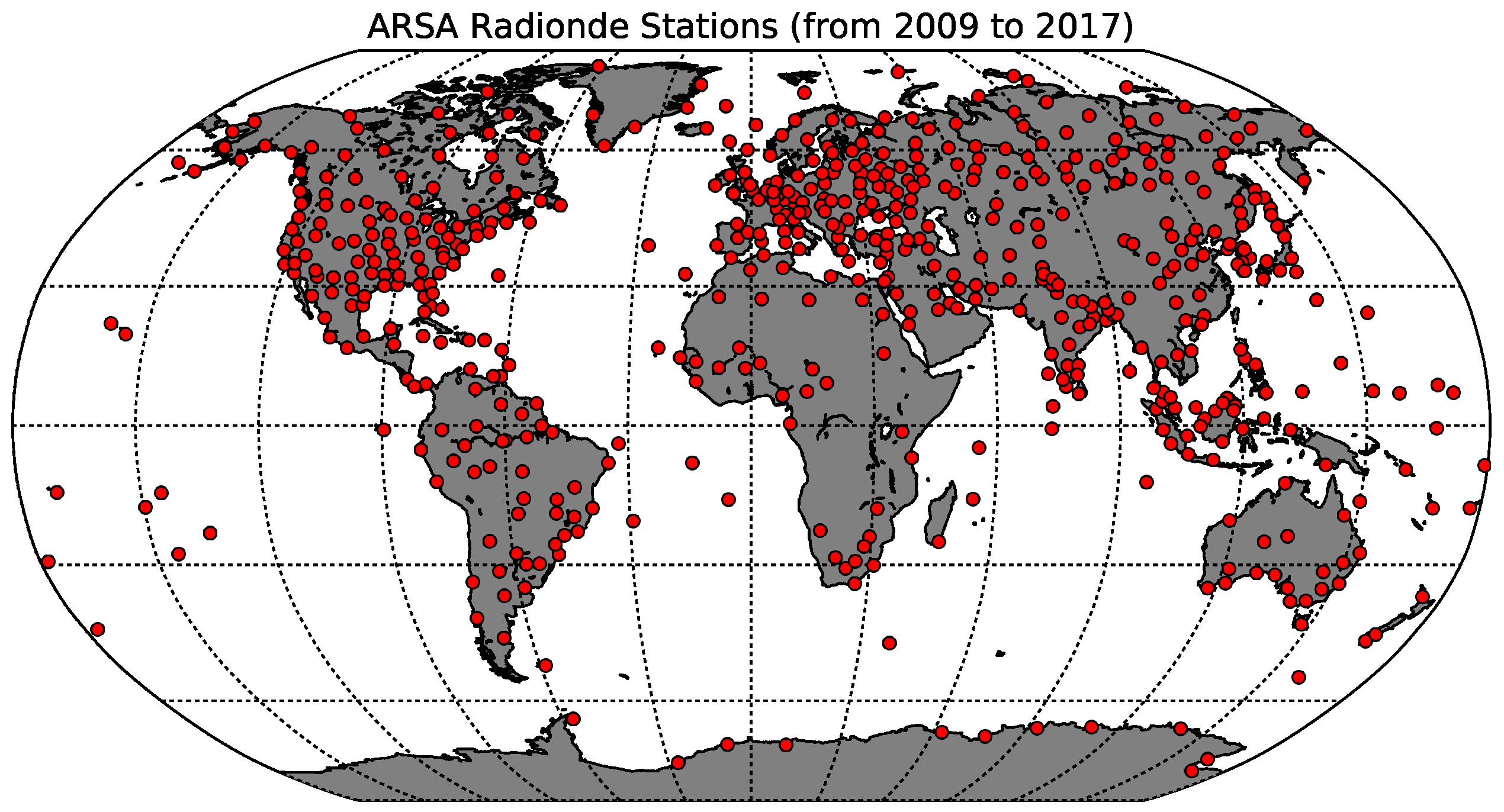
Figure 6.
Comparison of mean ARSA PBL calculated using the mixing layer height (MLH) derived from; (i) the original radiosonde profile (MLH1), (ii) the partial column top pressure (PCTP) and (iii) MLH derived from the radiosonde profile on the GOSAT retrieval grid (MLH2) as a function of latitude are shown in (a). The mean ratio of the PBL calculated from the PCTP relative to the MLH as a function of latitude are shown in (b). The global mean ratios of PCTP to MLH1 and MLH2 are 1.13 and 1.09 respectively. The mean differences between the PCTP and MLH as a function of latitude are shown in (c). All shaded regions and error bars are the respective standard error for each latitudinal bin.

Figure 7.
Seasonal distribution of GOSAT PBL XH2O for northern hemisphere (a) winter—December, January and February, (c) spring—March, April and May, (e) summer—June, July and August, and (g) autumn—September, October and November. The corresponding mean seasonal PBL partial column top pressure (PCTP) level values are also shown (b,d,f,h). Seasonal plots are based on mean values from December 2016 to November 2017, and are binned in to 5° × 5° averages. The variable spatial sampling of GOSAT introduces a strong seasonal signal, especially over sun glint oceans.

Figure 8.
Seasonal comparisons of GOSAT PBL XH2O with ARSA radiosonde matches for northern hemisphere; (a) winter—December, January and February, (b) spring—March, April and May, (c) summer—June, July and August, and (d) autumn—September, October and November. Matches are collated between June 2009 and May 2017 from GOSAT overpasses that are within 100 km of the ARSA station and ±30 min of launch. In addition to the linear fit (red line), the 2.5% and 97.5% confidence intervals (black dashed lines), the mean bias value (), the correlation (r), mean square error (MSE), error of the linear fit gradient (x) and number of matches are included for each season.

Figure 9.
Comparison of GOSAT PBL XH2O over 3 broad latitudinal bands for same 8 year collocation period (June 2009 to May 2017): (a) Tropics (±30°), (b) Mid-Latitudes (45°S–30°S, 30°N–45°N) and (c) High-Latitudes (>±45°).
Figure 9.
Comparison of GOSAT PBL XH2O over 3 broad latitudinal bands for same 8 year collocation period (June 2009 to May 2017): (a) Tropics (±30°), (b) Mid-Latitudes (45°S–30°S, 30°N–45°N) and (c) High-Latitudes (>±45°).

Figure 10.
Seasonal collocation and statistics for GOSAT and ARSA comparisons. Frames (a,c,e,g) show global distribution of matched cases as a function of season. North America, Central/Northern Asia and Europe can be seen as the dominate collocation areas. Frames (b,d,f,h) show the mean seasonal and global k (Equation (18)) value distributions. The majority of 5° × 5° cells reduce to below 2, i.e., they are in statistical agreement (Immler et al. [58]).


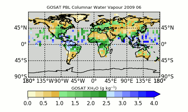
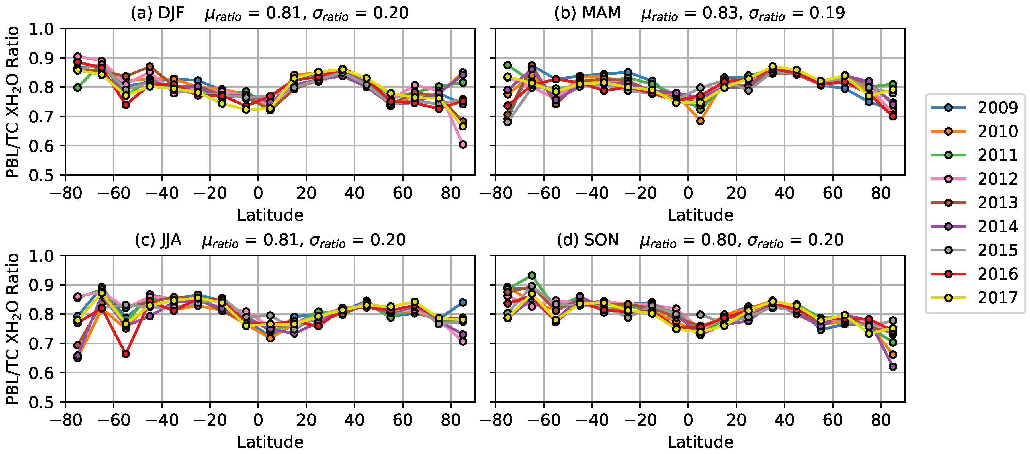
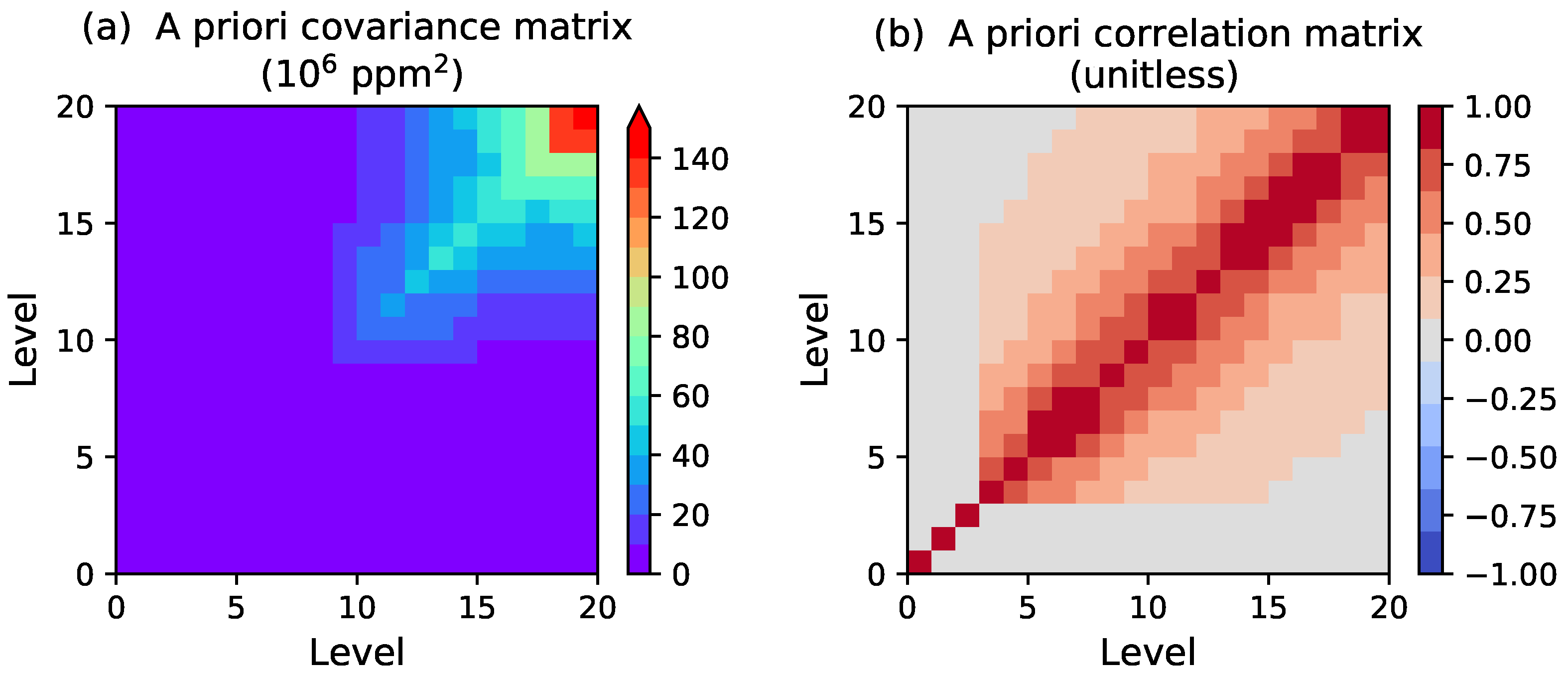
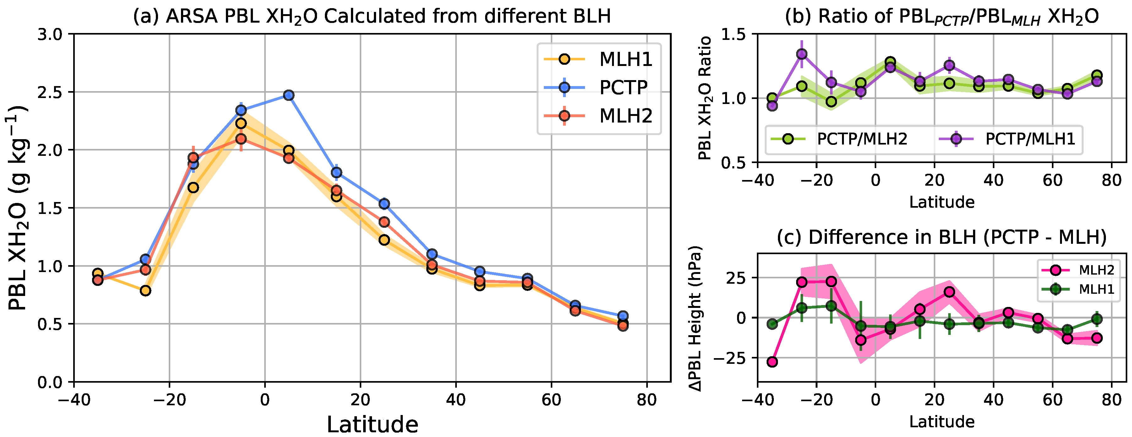
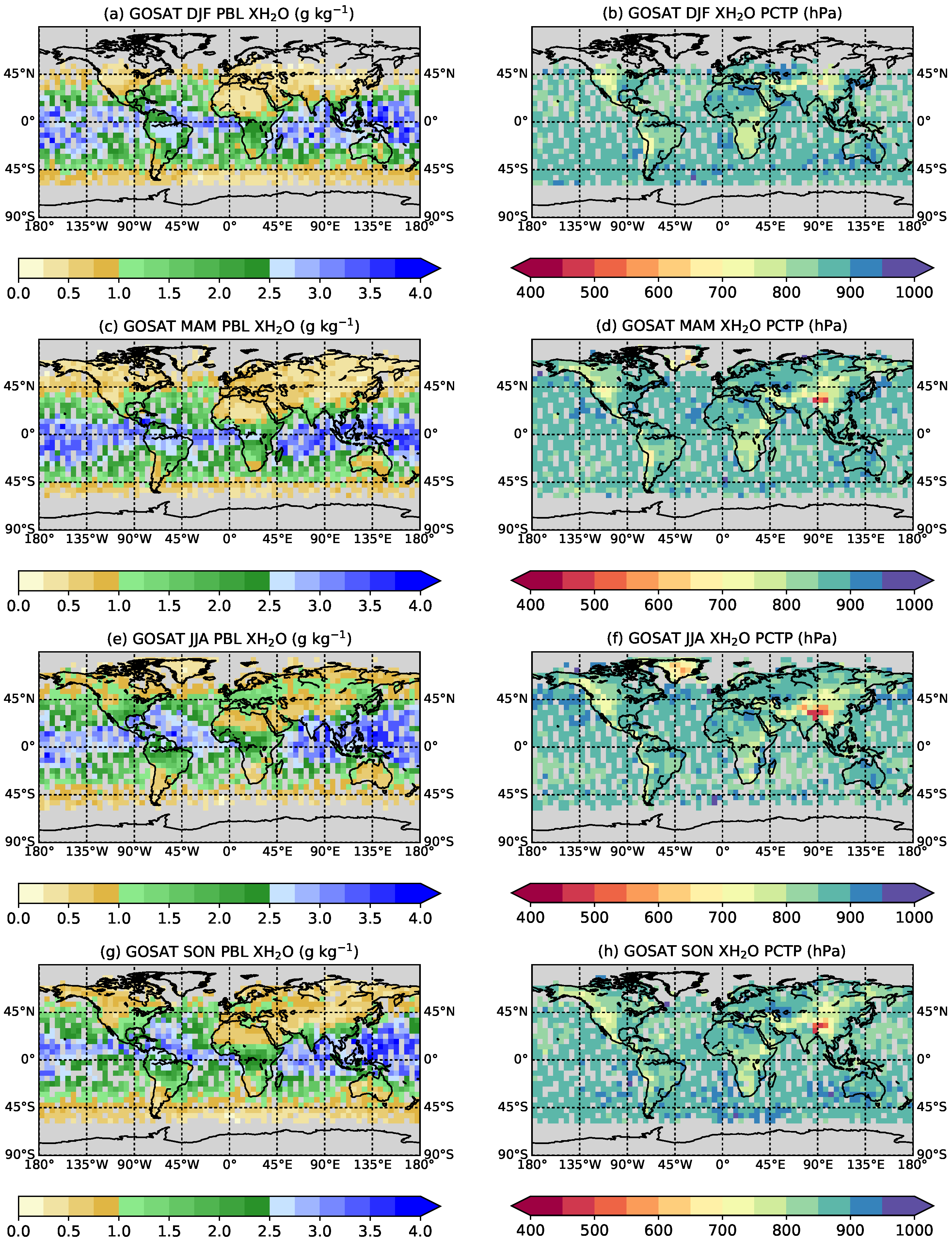
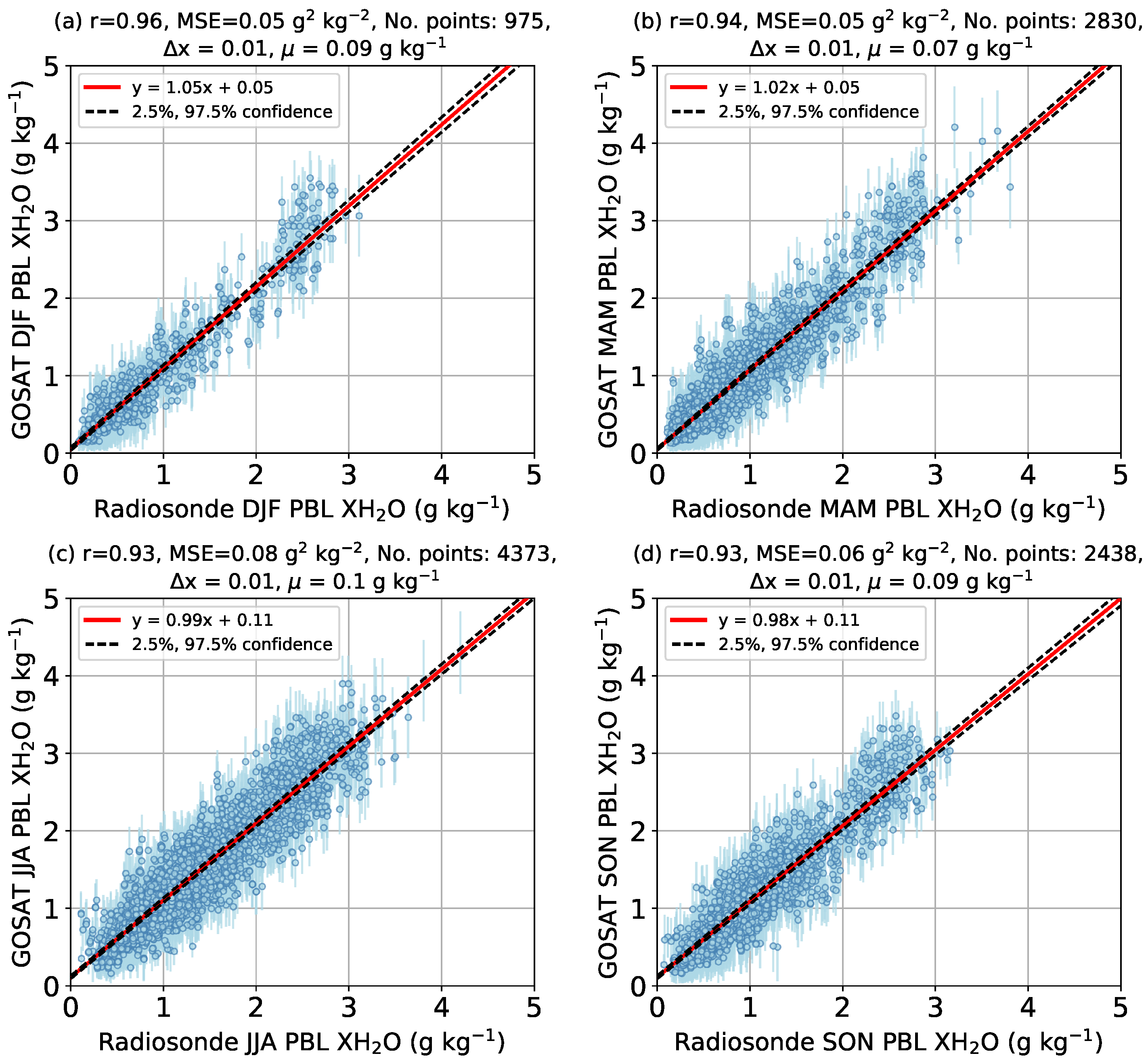
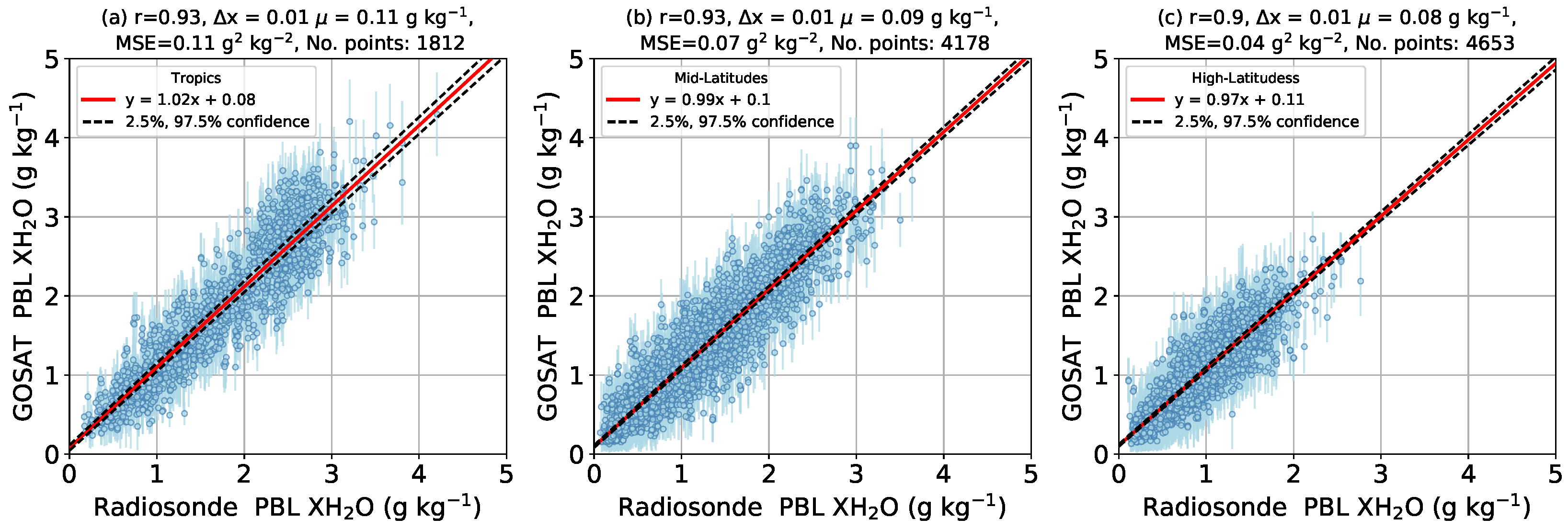
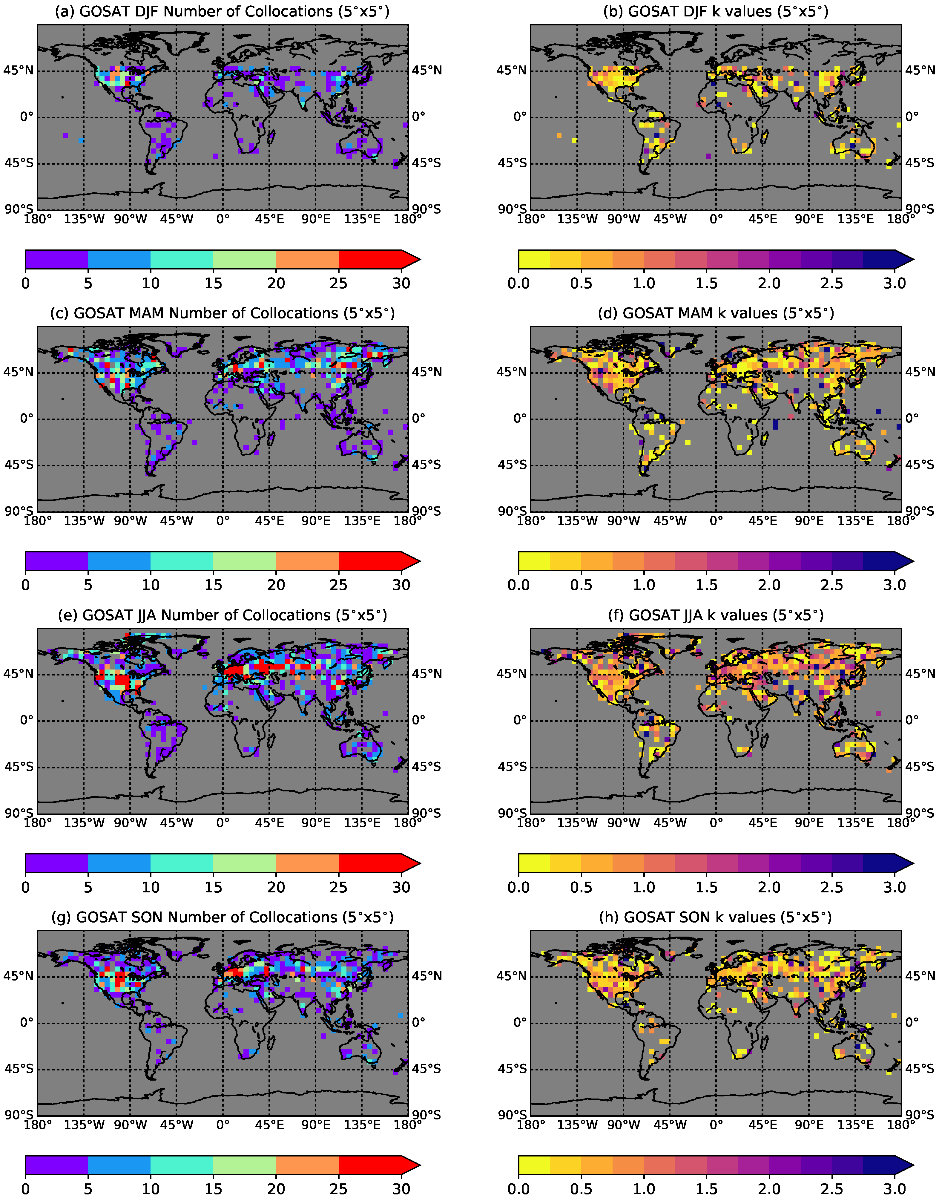
Table 1.
List of the non-target state vector variables for which interference uncertainties are calculated. The right-hand column displays the -funtion values used in calculating the interference values. B1, B2 and B3 refer to the GOSAT SWIR bands 1–3 respectively.
Table 1.
List of the non-target state vector variables for which interference uncertainties are calculated. The right-hand column displays the -funtion values used in calculating the interference values. B1, B2 and B3 refer to the GOSAT SWIR bands 1–3 respectively.
| Index Number () | Non-Target Variable | -Function |
|---|---|---|
| 1 | Carbon Dioxide (CO2) | 0.10 ppm |
| 2 | Methane (CH4) | 0.10 ppm |
| 3 | Surface Pressure (Psurf) | 4 hPa |
| 4 | Atmospheric Temperature (T) | 10.00 K |
| 5 | Aerosol Type 1 (mixture 4b, Kahn et al. [45]) | factor of 50 |
| 6 | Aerosol Type 2 (mixture 5b, Kahn et al. [45]) | factor of 50 |
| 7 | Cirrus Cloud | factor of 50 |
| 8 | Albedo (slope, offset) | 1.00, 1.75 (B1) |
| 1.00, 1.07 (B2) | ||
| 1.00, 1.13 (B3) |
Table 2.
Retrieval uncertainty components in g/kg and percentage of the retrieved PBL for 5 climatic regions. The a posterior uncertainties () are the far left-hand column of values, while the updated total retrieval uncertainties () are contained in the far right-hand column.
Table 2.
Retrieval uncertainty components in g/kg and percentage of the retrieved PBL for 5 climatic regions. The a posterior uncertainties () are the far left-hand column of values, while the updated total retrieval uncertainties () are contained in the far right-hand column.
| Region | ||||||||||
|---|---|---|---|---|---|---|---|---|---|---|
| g/kg | % | g/kg | % | g/kg | % | g/kg | % | g/kg | % | |
| Sahara Desert | 0.31 | 11.09 | 0.12 | 4.15 | 0.09 | 3.07 | 0.04 | 1.47 | 0.24 | 8.70 |
| Amazon | 0.31 | 10.04 | 0.09 | 3.00 | 0.09 | 2.77 | 0.02 | 0.78 | 0.20 | 6.55 |
| Europe | 0.30 | 16.84 | 0.10 | 5.80 | 0.07 | 4.22 | 0.03 | 1.47 | 0.20 | 11.49 |
| Greenland | 0.29 | 37.36 | 0.07 | 9.49 | 0.04 | 4.72 | 0.01 | 1.24 | 0.12 | 15.46 |
| Sun-Glint Pacific | 0.35 | 9.08 | 0.09 | 2.45 | 0.11 | 2.75 | 0.02 | 0.45 | 0.22 | 5.65 |
Table 3.
Decomposition of the interference error in to the individual contributions from the non-target state vector elements for the five sample regions. Values are presented as percentages of only.
Table 3.
Decomposition of the interference error in to the individual contributions from the non-target state vector elements for the five sample regions. Values are presented as percentages of only.
| Region | % Contribution of Total | |||||||
|---|---|---|---|---|---|---|---|---|
| CO2 | CH4 | Psurf | T | Aerosol Type 1 | Aerosol Type 2 | Cirrus Cloud | Albedo | |
| Sahara Desert | 0.57 | 0.27 | 0.43 | 3.07 | 37.12 | 43.59 | 14.59 | 0.36 |
| Amazon | 0.74 | 0.04 | 0.82 | 1.46 | 67.42 | 26.68 | 2.56 | 0.28 |
| Europe | 0.4 | 0.23 | 0.27 | 5.35 | 37.72 | 35.84 | 20.1 | 0.1 |
| Greenland | 0.81 | 0.3 | 1.38 | 11.25 | 19.12 | 11.97 | 55.01 | 0.17 |
| Sun-Glint Pacific | 0.75 | 0.16 | 0.87 | 1.47 | 60.69 | 32.64 | 3.21 | 0.22 |
© 2018 by the authors. Licensee MDPI, Basel, Switzerland. This article is an open access article distributed under the terms and conditions of the Creative Commons Attribution (CC BY) license (http://creativecommons.org/licenses/by/4.0/).
Share and Cite
MDPI and ACS Style
Trent, T.; Boesch, H.; Somkuti, P.; Scott, N.A. Observing Water Vapour in the Planetary Boundary Layer from the Short-Wave Infrared. Remote Sens. 2018, 10, 1469. https://doi.org/10.3390/rs10091469
AMA Style
Trent T, Boesch H, Somkuti P, Scott NA. Observing Water Vapour in the Planetary Boundary Layer from the Short-Wave Infrared. Remote Sensing. 2018; 10(9):1469. https://doi.org/10.3390/rs10091469
Chicago/Turabian StyleTrent, Tim, Hartmut Boesch, Peter Somkuti, and Noëlle A. Scott. 2018. "Observing Water Vapour in the Planetary Boundary Layer from the Short-Wave Infrared" Remote Sensing 10, no. 9: 1469. https://doi.org/10.3390/rs10091469
Note that from the first issue of 2016, this journal uses article numbers instead of page numbers. See further details here.