Comparisons of Spatially Downscaling TMPA and IMERG over the Tibetan Plateau

1
Institute of Remote Sensing and Geographic Information System, School of Earth and Space Science, Peking University, Beijing 100871, China
2
Institute of Agricultural Remote Sensing and Information Technology Application, College of Environmental and Resource Sciences, Zhejiang University, Hangzhou 310058, China
3
School of Civil Engineering and Environmental Science, University of Oklahoma, Norman, OK 73019, USA
*
Authors to whom correspondence should be addressed.
Remote Sens. 2018, 10(12), 1883; https://doi.org/10.3390/rs10121883
Submission received: 25 October 2018
/
Revised: 15 November 2018
/
Accepted: 16 November 2018
/
Published: 26 November 2018
(This article belongs to the Special Issue Remote Sensing Water Cycle: Theory, Sensors, Data, and Applications)
Abstract
:Accurate precipitation data is crucial in many applications such as hydrology, meteorology, and ecology. Compared with ground observations, satellite-based precipitation estimates can provide much more spatial information to characterize precipitation. In this study, the satellite-based precipitation products of Integrated Multi-satellitE Retrievals for Global Precipitation Measurement (IMERG) and Tropical Rainfall Measurement Mission (TRMM) Multisatellite Precipitation Analysis (TMPA) were firstly evaluated over the Tibetan Plateau (TP) in 2015 against ground observations at both annual and monthly scales. Secondly, random forest algorithm was used to obtain the annual downscaled results (~1 km) based on IMERG and TMPA data and the downscaled results were examined against rain gauge data. Thirdly, a disaggregation algorithm was used to obtain the monthly downscaled results based on those at annual scale. The results indicated that (1) IMERG performed better than TMPA at both annual and monthly scales; (2) IMERG had few anomalies while TMPA displayed significant numbers of outliers in central and western parts of the TP; (3) random forest was a promising algorithm in acquiring high resolution precipitation data with improved accuracy; (4) the downscaled results based on IMERG had better performances than those based on TMPA.
1. Introduction
Precipitation plays a significant role in global water cycles and energy exchanges [1]. Accurate precipitation information is highly desirable in various scientific and application fields such as water resource management, weather prediction, as well as disaster monitoring and control [2]. Currently, there are three kinds of independent instruments to obtaining precipitation data, including gauges, weather radar and satellite-based sensors [3]. Though conventional point-based measurements from rain gauges could provide relatively accurate rainfall values at the point scale, they are not suitable for providing continuous spatial precipitation distributions [4]. Weather radar can obtain rainfall data with finer spatiotemporal resolutions. However, weather radar has disadvantages due to errors from various sources such as beam blockage in complex terrain and range degradation issues [5]. While satellite-based remote sensing has great potentials to provide comprehensive estimates of precipitation globally with reasonable spatiotemporal resolutions and accuracy.
Several projects, including the Global Precipitation Climatology Project (GPCP) [6,7,8], the Global Satellite Mapping of Precipitation (GsMaP) project [9], and the Tropical Rainfall Measuring Mission (TRMM) [10,11,12], had calculated satellite-based precipitation estimates and published various precipitation products with different temporal and spatial resolutions for free, such as the TRMM Multisatellite Precipitation Analysis (TMPA) data set [12]. The TRMM, carrying a signal-frequency precipitation radar (PR; the Ku-band at 13.8 GHz) and a multichannel TRMM Microwave Imager (TMI; frequencies range between 10 and 85.5 GHz), had provided a range of precipitation products since 1997 [10] and intended to provide the ‘best’ satellite precipitation estimates [12]. TMPA data had been widely applied in various fields, such as hydrological modeling [13], flood prediction [14] and climatology [15], over the past two decades.
With the success of TRMM, the Global Precipitation Measurement (GPM) Core Observatory was launched in February 2014 by a joint effort of the National Aeronautics and Space Administration (NASA) and the Japan Aerospace Exploration Agency (JAXA). The GPM Core Observatory carried a dual-frequency precipitation radar (DPR; the Ku-band at 13.6 GHz and Ka-band at 35.5 GHz) and a conical-scanning multichannel GPM Microwave Imager (GMI; frequencies range between 10 and 183 GHz). Compared with TRMM’s instruments, GPM extended its sensor packages and could detect light and solid precipitation more accurately than TRMM sensors [2,16]. Numerous studies had examined the accuracy of GPM rainfall products. The performance of the Integrated Multi-satellitE Retrievals for GPM (IMERG) and TMPA products were evaluated over mainland China at various spatiotemporal resolutions [17]. In southeast India, the accuracy of IMERG data were validated and compared with those of TMPA and GsMaP data [18]. While in Far East Asia, the IMERG and TMAP data were employed to evaluate the topographical and seasonal precipitation features applied [19]. These studies mainly demonstrated that IMERG had a better ability to provide more accurate rainfall estimate data than TMPA data.
However, the spatial resolution of TMPA data was too coarse (0.25°) and could not meet the demands of some researches, especially at the regional and basin scales. As a result, numerous downscaling models combining different environmental variables as auxiliary data had been explored to derive precipitation estimates at 1 km scale. To downscale TMPA data, the exponential regression model between TMPA and the normalized difference vegetation index (NDVI) was firstly applied in [20]. Based on this downscaling method, a statistical regression downscaling algorithm, introducing the NDVI and the digital elevation model (DEM), was developed [21]. The regression kriging method was also found to be feasible to downscale TMPA data [22]. While in [23], a downscaling algorithm namely geographically weighted regression (GWR) was introduced, which considered a regional regression model. Recently, a spatial data mining algorithm which introduced a series of land surface variables (NDVI, land surface temperature (LST) for both day (LST-d) and night (LST-n), DEM, etc.) was proposed [24,25]. While the resolution of IMERG was still too coarse (0.1°), and it was important to downscale IMERG data into a finer resolution (~1 km) for applications at the regional or basin scales. Many studies had evaluated the quality and accuracy of IMERG data, but few focused on the downscaling performance of IMERG.
Random forest (RF) is a nonparametric statistical regression algorithm developed from classification and regression tree (CART). In this study, the IMERG and TMPA data were explored to obtain downscaled results at the 1 km scale based on the nonparametric regression models constructed using the RF model. Moreover, both the original satellite-based precipitation estimates (TMPA and IMERG) and the downscaled results were furtherly analyzed and compared to reveal their differences at different spatial scales.
The objectives of this study were as follows: (1) to compare the quality of TMPA and IMERG over the TP at both annual and monthly temporal scales against ground observations; (2) to obtain downscaled results (~1 km) based on TMPA and IMERG data, respectively; and (3) to generate the monthly downscaled results based on those at annual scale.
2. Materials and Methods
2.1. Study Area
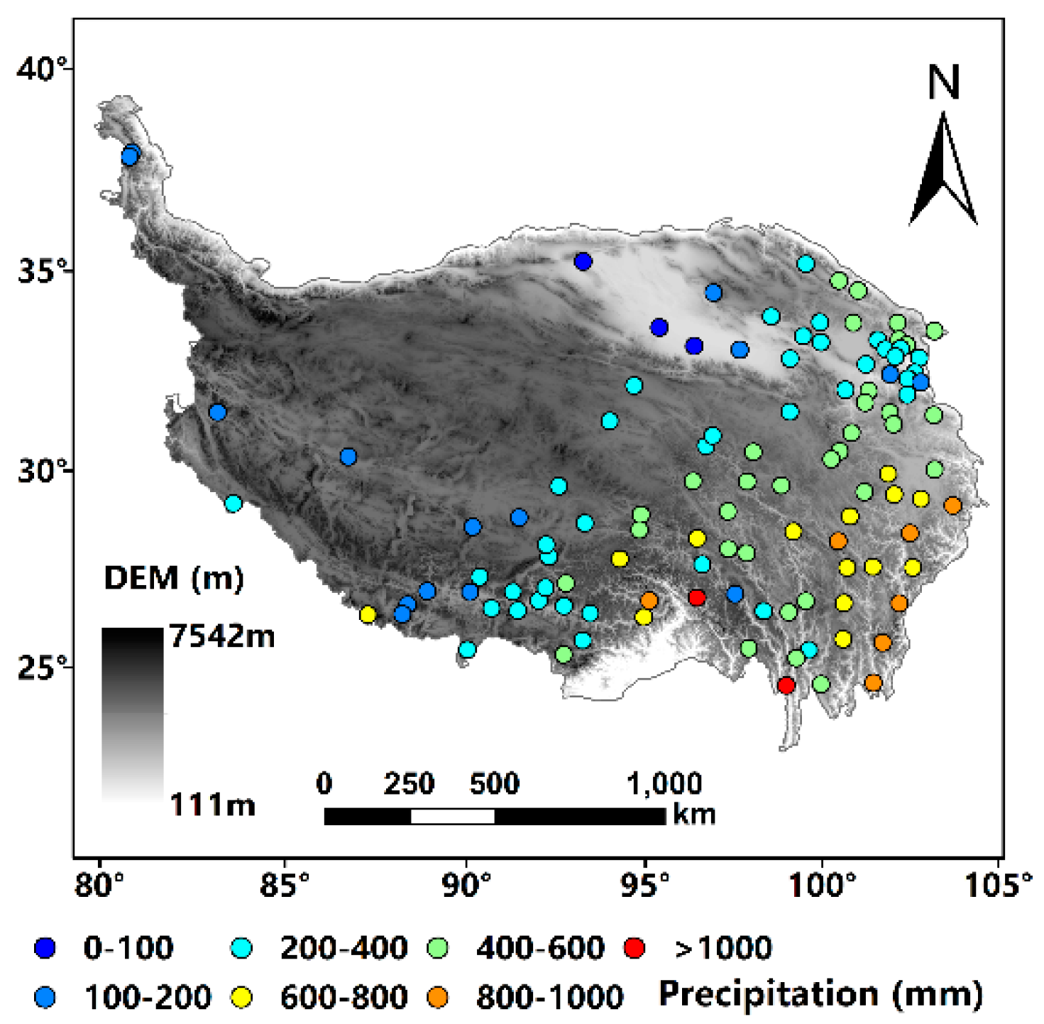
The TP is located in southwestern China (Figure 1) between 73°–104° E and 26°–40°N. It is the highest plateau on Earth. The extent of the TP is approximately 2.5 million km2, with an average elevation of >4000 m above mean sea level. Because of the complex topography and extremely high elevation, the precipitation on the TP exhibits substantial spatiotemporal variability [26]. Spatially, much of the precipitation occurs in the central and southern parts of the plateau, with little in the western and northern parts. Temporally, the amount of rainfall differs seasonally. Spring and summer receive approximately 90% of the annual precipitation because of the effects of the Indian monsoon, which brings substantial water vapor from the sea. In winter, the westerlies influence the western part of the plateau, resulting in little rainfall. The TP contains the upstream reaches of the five major Asian rivers, including the Yellow, Brahmaputra, Ganges, Indus and Yangtze Rivers [27,28], which supply water resources for more than 1.4 billion people [29].
2.2. Materials
2.2.1. Rain Gauges
The rain gauge data used in this study were provided by the Third Pole Environment Database (http://en.tpedatabase.cn/portal/MetaDataInfo.jsp?MetaDataId=249472). This dataset provided daily precipitation data from 1979 to 2015 for the TP and its surroundings. We obtained precipitation records from 113 rain gauge stations which distributed unevenly across the TP (Figure 1). Daily precipitation records from January 2015 through December 2015 were used in this study. The monthly and annual precipitation volume for each station were calculated by accumulating the daily precipitation.
2.2.2. TRMM Satellite Precipitation Dataset
The TRMM was launched in November 1997 through cooperation between NASA and JAXA to monitor and investigate tropical and subtropical rainfall system. The TMPA employed inputs from two different types of satellite sensors. The primary data source was from precipitation-related microwave sensors, including the TMI, Special Sensor Microwave/Imager (SSM/I) and Special Sensor Microwave Imager/Sounder (SSMIS), Advanced Microwave Scanning Radiometer for the Earth Observing System (AMSR-E), the Advanced Microwave Sounding Unit (AMSU) and the Microwave Humidity Sounders (MHS). Additionally, the second major data source for the TMPA was the geo-infrared (IR) data. Precipitation information collected from these sensors were combined to generate precipitation estimates. The TMPA 3B43 Version 7 monthly precipitation products were published for free at a spatial resolution of for latitudes from 50° N–50° S worldwide [12]. The TMPA 3B43 V7 spanning from January 2015 to December 2015 were employed in this study and it were obtained from the Precipitation Measurement Mission (PMM) website (http://pmm.nasa.gov/data-access/downloads/trmm). Annual precipitation was obtained by accumulating monthly TMPA precipitation in the year.
2.2.3. IMERG Satellite Precipitation Dataset
GPM is an international project that launched on 27 February 2014 by a joint effort of NASA and JAXA. It was designed to provide a new generation of global precipitation observations. IMERG is the level 3 multi-satellite precipitation algorithm of GPM, which combined precipitation information obtained from all constellation microwave sensors, infrared-based observations and monthly gauge precipitation data [2]. IMERG employs the 2014 version of the Goddard Profiling Algorithm (GPROF2014) to compute precipitation estimates from all passive microwave (PMW) sensors onboard GPM satellites constellation which was one of the significant improvements compared with TMPA (GPROF2010) [16,30]. The GPM-3IMERGM ‘Final’ V05B product (hereafter referred as IMERG), which estimated global monthly precipitation at spatial resolution of , were used in this study. Since IMERG data are available from March 2014, the first year with full months (i.e., 2015) was selected. IMERG data could be downloaded at http://pmm.nasa.gov/data-access/downloads/gpm. Furthermore, annual IMERG precipitation was obtained by summing up monthly precipitation in the year.
2.2.4. NDVI Datasets
The NDVI is typically used to determine the vegetation productivity and distribution [31,32], and is correlated well with precipitation at annual temporal scale [25,33,34]. The MOD13A3 monthly NDVI product from January 2015 to December 2015 with a spatial resolution of 1 km was employed in this study. The MOD13A3 was derived from atmospherically corrected reflectance in the red and near-infrared wavebands of the Moderate Resolution Imaging Spectroradiometer (MODIS) on the Terra satellite, which can be downloaded at https://ladsweb.modaps.eosdis.nasa.gov/search/. Annual NDVI value was obtained by averaging monthly NDVI in the year.
2.2.5. Land Surface Temperature Datasets
Land surface temperature datasets were collected through MODIS sensors aboard the Terra and Aqua satellites. MODIS can provide the global land surface temperature records of day and night with an error-controlled between −1 K and 1 K. MODIS11A2 products with a spatial resolution of 1 km and an eight-day temporal resolution were obtained at (https://lpdaac.usgs.gov/dataset_discovery/modis/modis_products_table/mod11a2_v006). In 2015, there were forty-five 8-day periods, we calculated the averaged day and night land surface temperatures over the TP to determine the year-round land surface temperature for day (LST-d) and night (LST-n).
2.2.6. Topography Datasets
The Shuttle Radar Topography Mission (SRTM) is an international project spearheaded by the National Geospatial-Intelligence Agency (NGA) and (NASA), and it was launched in February 2000. The SRTM project provided high-resolution DEM data with a spatial coverage ranging from 56°S to 60°N and a spatial resolution of one arc second (~30 m). In this study, the dataset with three arcs second (approximately 90 m) were adopted as the basic topographical data (http://srtm.csi.cgiar.org). Other topographical parameters, including slope [35], aspect [36], curvature [37], radiation [38], slope length and steepness (LS) [39], the topographic wetness index (TWI) [40], the multiresolution valley bottom flatness index (MrVBF) [41] and the terrain ruggedness index [42], were derived from DEM data. Curvature, radiation, and ruggedness were abbreviated as Curv, Radi, and Rugg, respectively.
2.3. Methods
2.3.1. Random Forest
RF was developed as an extension of the CART to improve the accuracy and stability of the CART model [43]. To perform a regression in CART, the model searches every distinct value of every predictor in the entire data set (S) to find the optimal predictor and split values that are used to partition the data into two groups (S1 and S2), such that the overall sum of squared error (SSE) is minimized [44]:
where and represent the averages of the training set outcomes of groups S1 and S2, respectively. The process continues within sets S1 and S2 until the number of samples in the splits falls below some threshold.
To reduce the variance of the estimates, bagging (short for bootstrap aggregation) strategy was proposed. The bagging method generates m bootstrap samples of the original data and trains the tree model for each bootstrap sample. Each model is then used to generate a prediction for a new sample, and these m predictions are averaged to obtain the bagged model’s prediction. However, the trees in bagging are not completely independent of each other because of the underlying relationship between the predictors and responses. The trees from different bootstrap samples may have similar structures that prevent bagging from optimally reducing the variance of the predicted values. Random Forest was developed to reduce the tree correlation by randomly selecting predictors at each split.
The main steps of the random forest algorithm were as follows.
- (1)
- To randomly generate ntree bootstrap samples from the original dataset. The elements not selected are referred to as ‘out of bag’ (OOB) samples.
- (2)
- For each split, to randomly select predictors of the original predictors and choose the best predictor among the predictors to partition the dataset. Additionally, is the tuning parameter of the model.
- (3)
- To predict new data (OOB elements) by averaging predictions of the ntree trees.
- (4)
- The OOB samples were used to estimate the prediction error. The OOB estimate of the error rate [45] was calculated as follows:where represents the observation of the ith OOB prediction.
The random forest can provide a measurement of variable’s importance. One of the approaches is to look at the increase in the OOB estimate error when the specific predictor variable is randomly permuted and other predictors are kept unchanged. The more the error increases, the more important the variable is. These variable importance values are used to rank the predictors in terms of their relative contribution to the model. The random forest model was generated using the package randomforest in R (https://cran.r-project.org/web/packages/randomForest/).
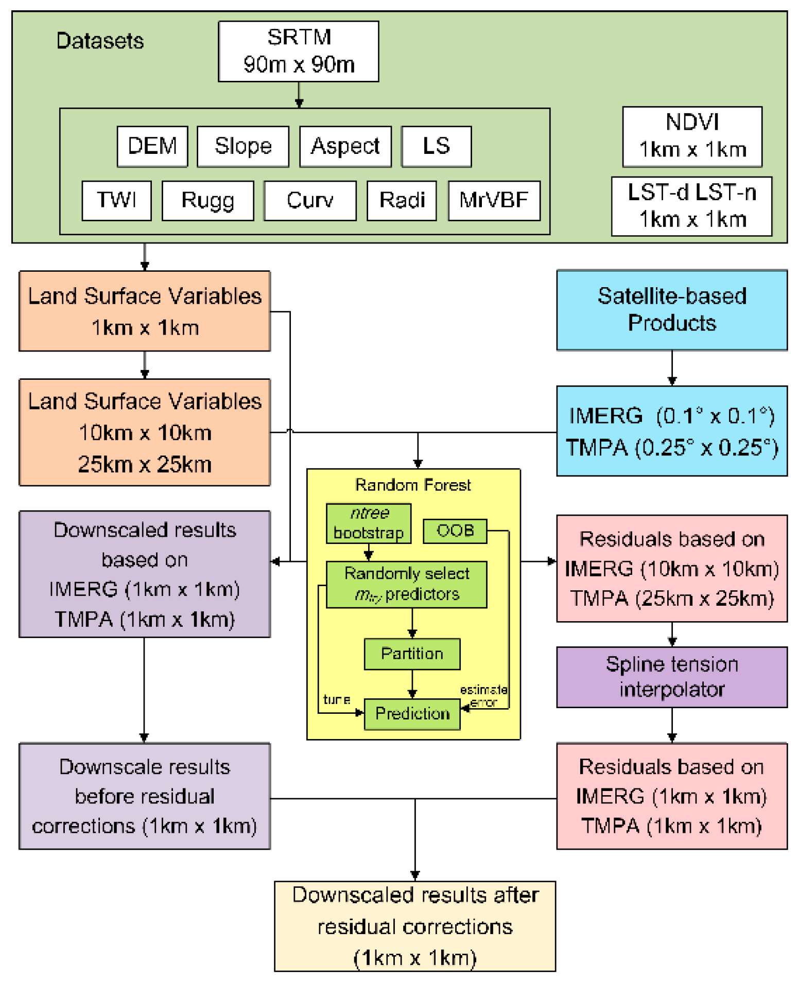
2.3.2. Main Downscaling Steps at the Annual Scale
RF was used to downscale the TMPA and IMERG data over the TP at an annual scale. The main steps in the downscaling process were as follows:
- (1)
- Sum the TMPA and IMERG monthly precipitation to annual precipitation ().
- (2)
- Aggregate land surface variables with their original resolutions to those at the resolutions of 0.1° and 0.25°, respectively.
- (3)
- Establish the random forest model between land surface variables at 0.25° and , and establish the random forest model between land surface variables at 0.1° and .
- (4)
- Estimate annual precipitation at 0.25° using , and estimate annual precipitation at 0.1° using .
- (5)
- Map the residuals at 0.25° () by computing the difference between and the estimated annual precipitation at 0.25°. Similarly, map the residuals at 0.1° () by computing the difference between and the estimated annual precipitation at 0.1°.
- (6)
- Obtain the residuals ( and ) at 1 km from those at 0.25° using a simple spline tension interpolator. As the residual data were regularly spaced, the spline interpolation was typically used for this type of data.
- (7)
- Generate the annual precipitation estimates, termed as the downscaled results before residual corrections, at 1 km using and , respectively, in combination with the land surface variables.
- (8)
- Add the residuals at 1 km obtained at step (6) and the downscaled results before residual corrections at 1 km obtained at step (7) to finally obtain the downscaled results after residual corrections.
The steps used for downscaling are shown in Figure 2.
2.3.3. Disaggregation from Annual Precipitation to Monthly Precipitation
Considering the time lag of the response of the NDVI to precipitation [46], we used a disaggregation algorithm to obtain the monthly downscaled results. The disaggregation algorithm was based on the assumption that the monthly ratios are as defined in Equation (3) [47].
The numerator represents the precipitation that occurs in the ith month estimated from the original satellite precipitation product, and the denominator represents the annual precipitation. Note that the spatial resolution of is the same as that of the original satellite precipitation data, and the ratios were further interpolated by spline interpolation to 1 km, which was consistent with the downscaled annual results. The monthly downscaled results can then be acquired by multiplying the monthly ratios (~1 km) by the annually downscaled results.
2.3.4. Validation
Validation statistics, including the coefficient of determination (R2), bias, the mean absolute error (MAE) and the root mean square error (RMSE) were used to access the performance of the original satellite-based precipitation products and the downscaled results against precipitation estimates observed from rain gauges. The R2 values indicate the strength of the linear relationship between the precipitation estimates and ground observations, ranging between 0 and 1 with an optimal value of 1. Bias denotes the degree either over- or underestimated, with a perfect value of 0. Overestimation is represented as positive bias indicating the satellite value is higher than gauge data. MAE shows the mean magnitude of the errors and RMSE was used to represent the distribution of errors. Smaller values of MAE and RMSE indicate more accurate and precise results. The perfect score for both the MAE and RMSE is 0.
where is the satellite precipitation measurement; is the measured precipitation from rain gauge stations; n is the total number of samples.
3. Results
3.1. Original Results and Validations Using Ground Observations at Annual and Monthly Scales
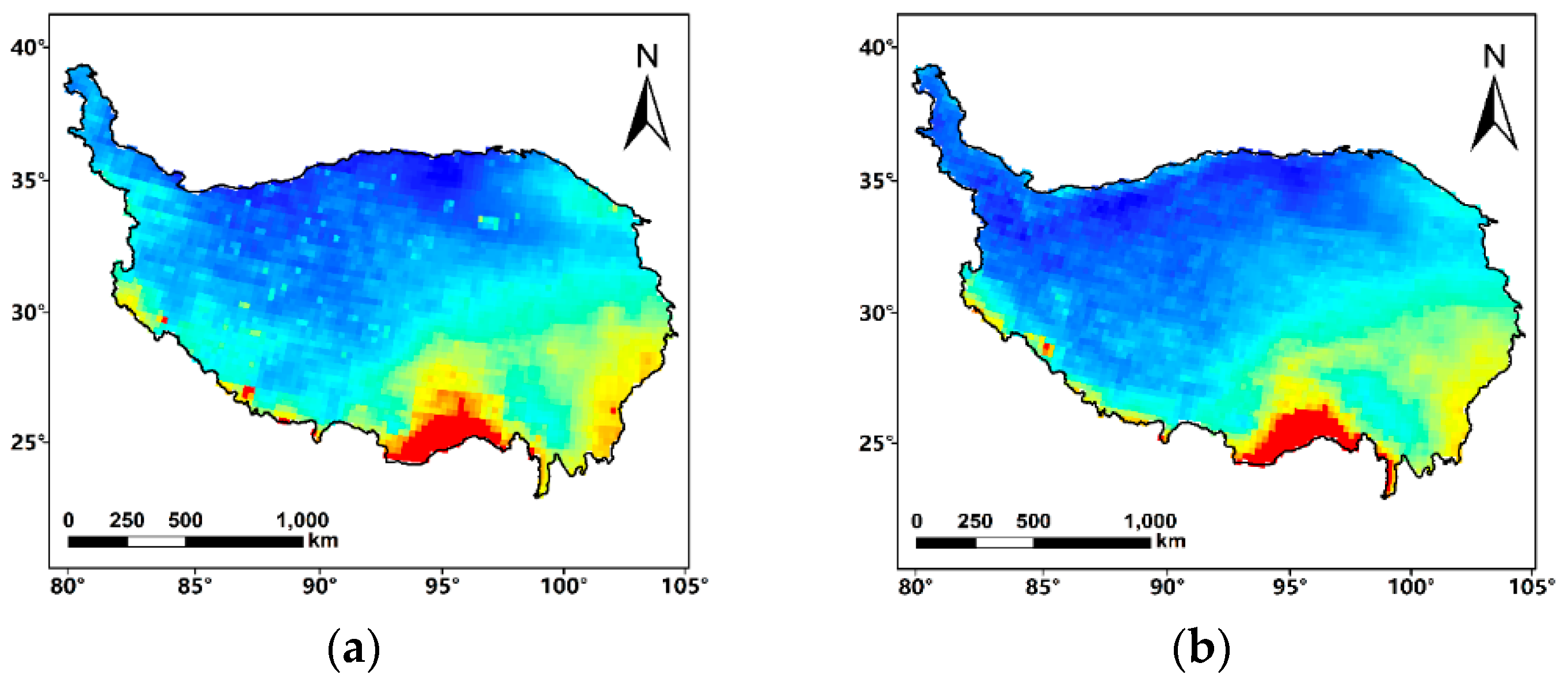
Figure 3a–c represented the annual precipitation maps derived from original TMPA, resampled IMERG and original IMERG in the year 2015 over the TP, respectively. Over the region, both TMPA and IMERG data, as well as the resampled IMERG, captured the typical southeast-northwest decreasing precipitation patterns, which were consistent with the patterns measured by rain gauges displayed in Figure 1. TMPA and IMERG patterns were close as they utilized similar sensors including IR and PMW sensors, to retrieve precipitation. However, TMPA presented some exceptional values in the western and northern parts of the TP relative to the neighboring pixels. These anomalies did not appear in IMERG estimates resulting in more continuous precipitation trends.
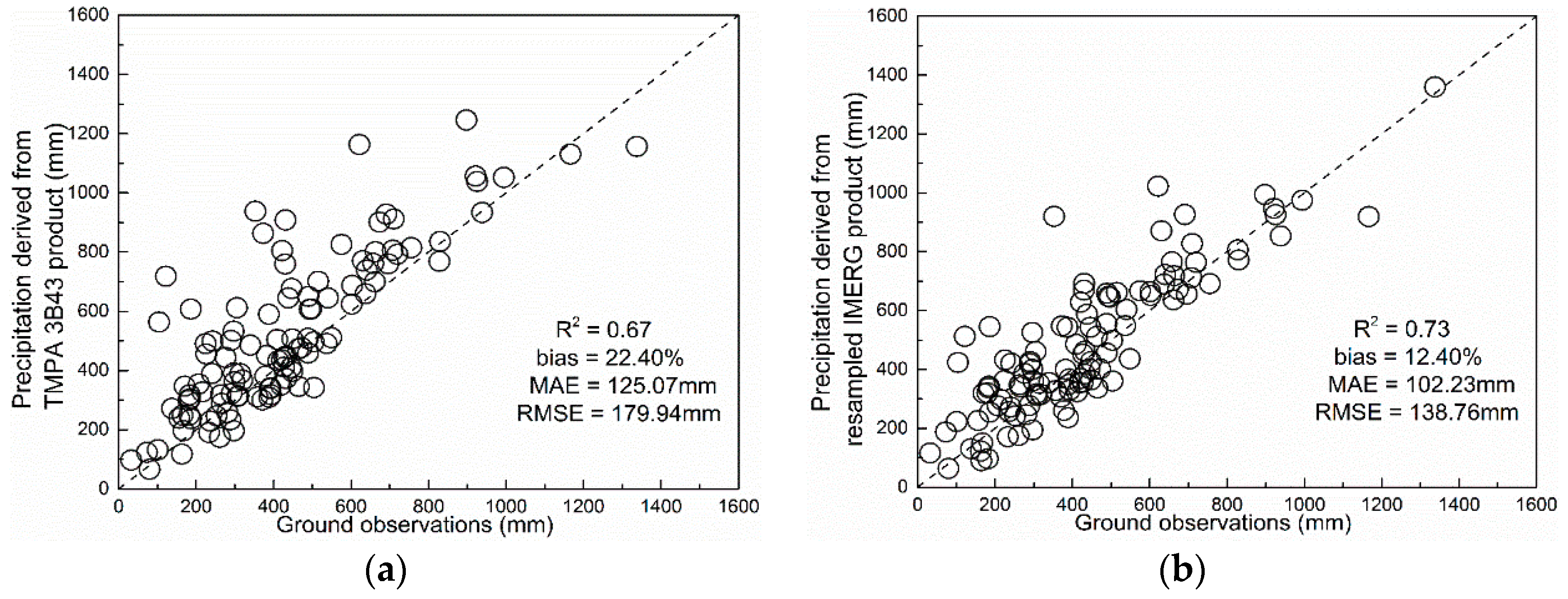
To compare the performance of the original TMPA data with resampled IMERG, as well as the original IMERG data, we validated these products against ground observations from 113 rain gauge stations on the TP in 2015. Figure 4a shown the scatterplot of the validation between ground observations and the original TMPA data at resolution. Figure 4b,c demonstrate the validations of resampled IMERG data at resolution and original IMERG data at resolution, against ground observations, respectively. Both satellite precipitation products generally overestimated precipitation over the TP compared to ground observations. The original TMPA was the mostly overestimated product compared to ground observations (R2 ~ 0.67, bias ~ 22.40%). IMERG shown improved accuracy (R2 ~ 0.74, bias ~ 12.23%) at resolution. The resampled IMERG data also outperformed the original TMPA data, with R2 ~ 0.73 and bias ~ 12.40%, at the same spatial resolution of .
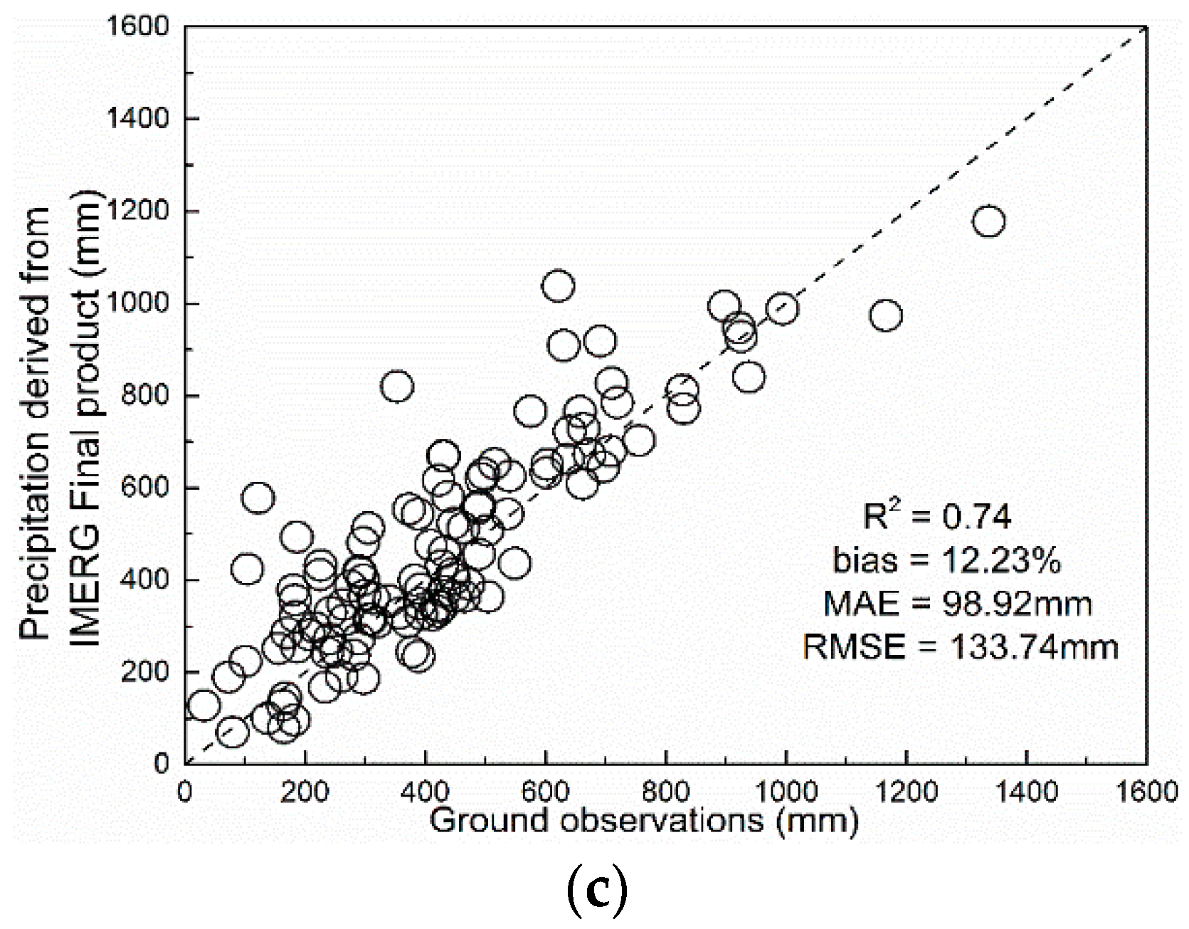
Figure 5 displayed the monthly mean precipitation from 113 rain gauges, the original TMPA, resampled IMERG and the original IMERG, respectively. Both TMPA and IMERG successfully captured the precipitation dynamics intra-annually, with heavy precipitation occurred at June, July, August and September (referred as wet seasons), while little precipitation happened in November, December, January and February (referred as dry seasons). IMERG estimates were better than TMPA estimates, due to its values were closer to the ground measured precipitation amounts.
Table 1 presented the statistical results at monthly scale. Both TMPA and IMERG products performed better during the wet seasons and performed worse during the dry seasons. During dry seasons, the volume of precipitation was lower, and the durations of the precipitation was shorter in time which made the detection more complicated by PWM sensor. The performance of IMERG was slightly better than TMPA during the dry seasons with relatively higher values of R2 and lower values of bias, MAE and RMSE, respectively. One of the possible reasons for the improvements may attribute to the extended sensors that equipped on IMERG (DPR and GMI) than sensors equipped on TMPA (PR and TMI), leading to a more accurate detection of light and solid precipitation. Another likely reason to explain why IMERG performed better than TMPA during the dry season was that the different PWM retrievals. IMERG employed the GPROF2014 while TMPA employed GPROF2010. GPROF2014 was Bayesian in nature, and used “dynamic” detection threshold values, compared with GPROF2010 of regression and relative “static” detection threshold values. Therefore, GPROF2014 resulted in much less “false” alarm. During wet seasons, both TMPA and IMERG corresponded well with ground observations with R2 values approximately 0.70. IMERG was still more accurate with bias ~ 10%, MAE ~ 22 mm and RMSE ~ 32 mm, than TMPA (bias ~ 20%, MAE ~ 25 mm, RMSE ~ 37 mm). Regrading to the resampled IMERG data at resolution, the statistical results were very close to those of the original IMERG at 0.1 and thus provided more accurate precipitation estimates than TMPA at . Based on these evaluations, we concluded that IMERG data were better than TMPA data in terms of accuracy, with anomalies removed at the annual scale.
3.2. Main Results in the Downscaling Procedure Using Random Forest
Ntree and were the key parameters that affected the predictive performances of the RF model. To determine the optimal selection of parameters, the OOB error rate, as defined in Equation (2), was applied. The OOB error rate was an internal estimate of the predictive performances provided by the bagging model. The values of OOB error usually correlated well with the assessment of the predictive performance obtained from a cross-validation or test set. In addition, using OOB error rate could decrease the computational time required to tune RF model.
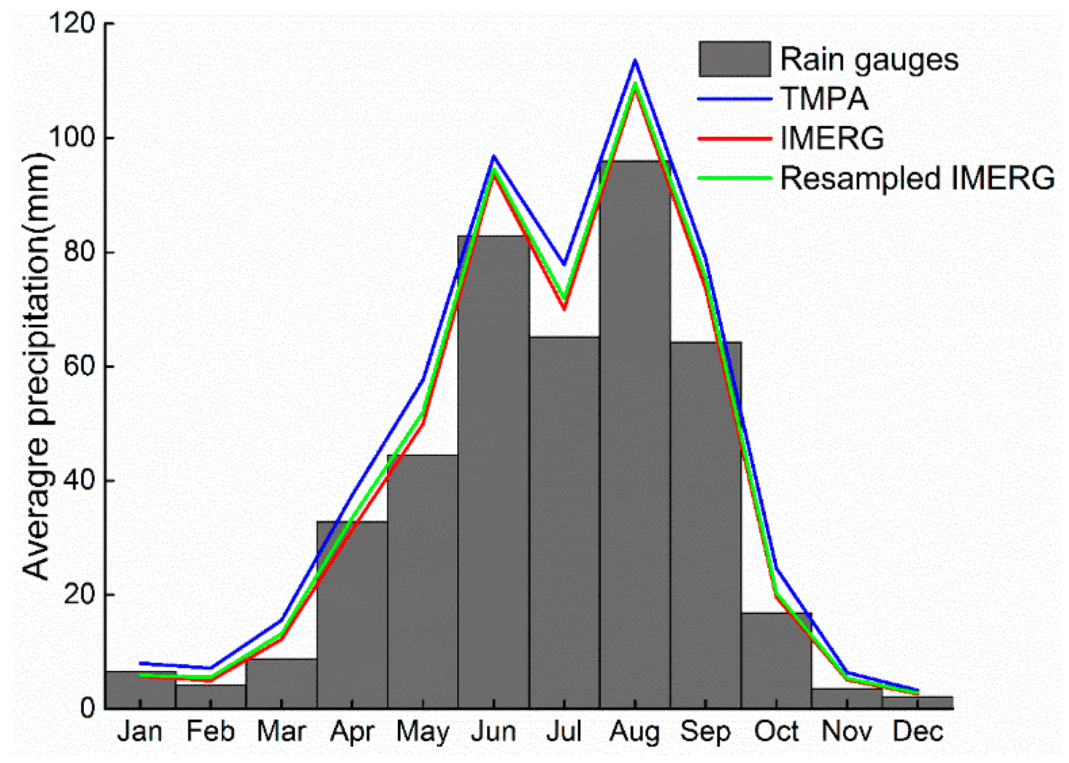
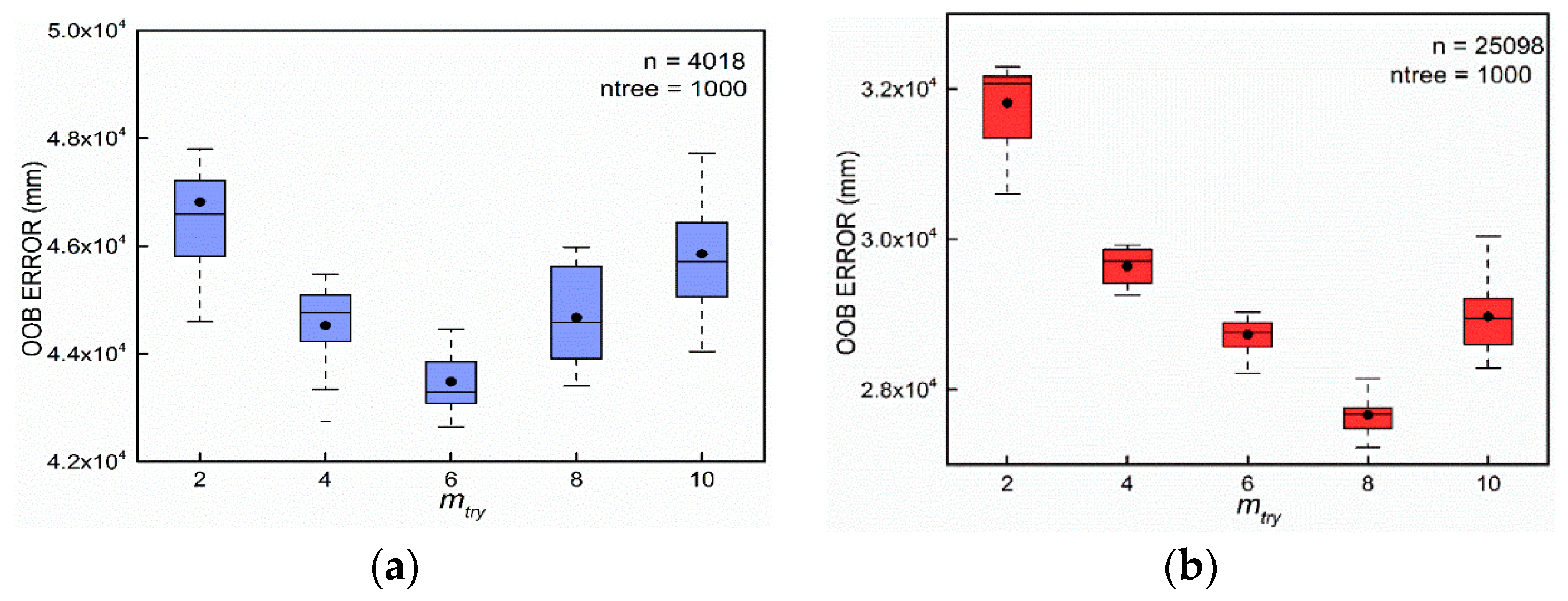
The RF was protected from overfitting [43], the model could not be adversely affected if a large number of trees were built for the forest. Figure 6a,b indicated that the OOB error in and decreased not significantly when ntree increased from 900 to 1500. To balance the accuracy and computational burden, 1000 was finally selected as the value of ntree for both and .
To specify the parameter for and , we tested five values of that ranged from 2 to 10 and independently generated 1000 tree models at each value. The boxplots of the OOB error for and were presented in Figure 7a,b, respectively. The upper and lower edges of the central box were the first and third quartiles (25% and 75%, respectively). The sign of band and circle inside the box represented the median and average value of OOB error, respectively. For , the OOB error decreased when the value of increased from 2 to 6 and then increased with increasing values from 6 to 10. For , the OOB error decreased when increased from 2 to 8. Therefore, a combination of ntree = 1000 and = 6 was applied to build the model and downscale the TMPA data, and ntree = 1000 and = 8 was employed to build the model and downscale the IMERG data over the TP.
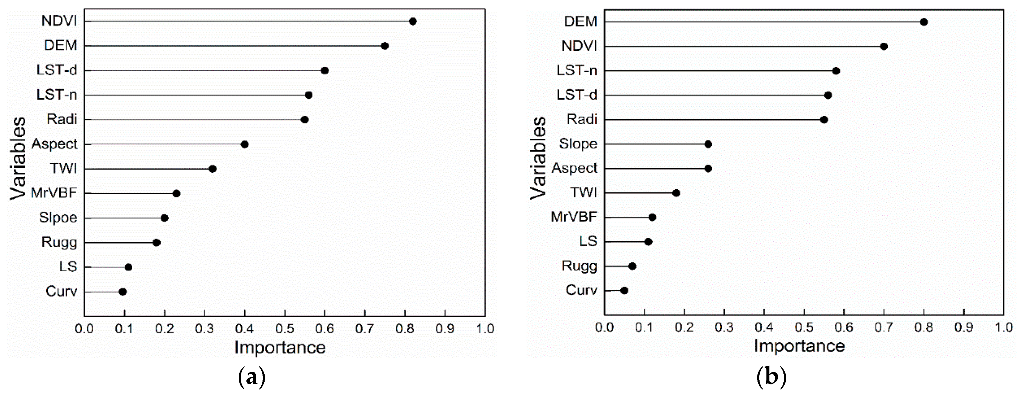
Figure 8a,b demonstrated the variable importance in and , respectively. These indicated that NDVI, DEM, LST-d and LST-n were the main factors contributed to establish the random forest models and that these factors influenced the spatial patterns and amount of precipitation at annual scale. The spatial distribution of the dominant factors which influenced the spatial distribution of precipitation over the TP was firstly explored in [25]. In central and northeast TP where were mainly covered by grassland and meadows (which were easily influenced by precipitation), the NDVI was the most important factor. The dominant factors were LST-d and LST-n in the northwest and west, where the temperatures were low with high elevations, and the precipitation in these regions could be influenced through thermal and dynamic mechanisms. In the southeast regions, topography played the most important roles in influencing the precipitation. Orographic rainfall typically occurred in the southeast where the topography varied greatly from valleys to huge mountains ranging in elevation from 100 to 4000 m.
3.3. Downscaled Results and Validations Using Ground Observations
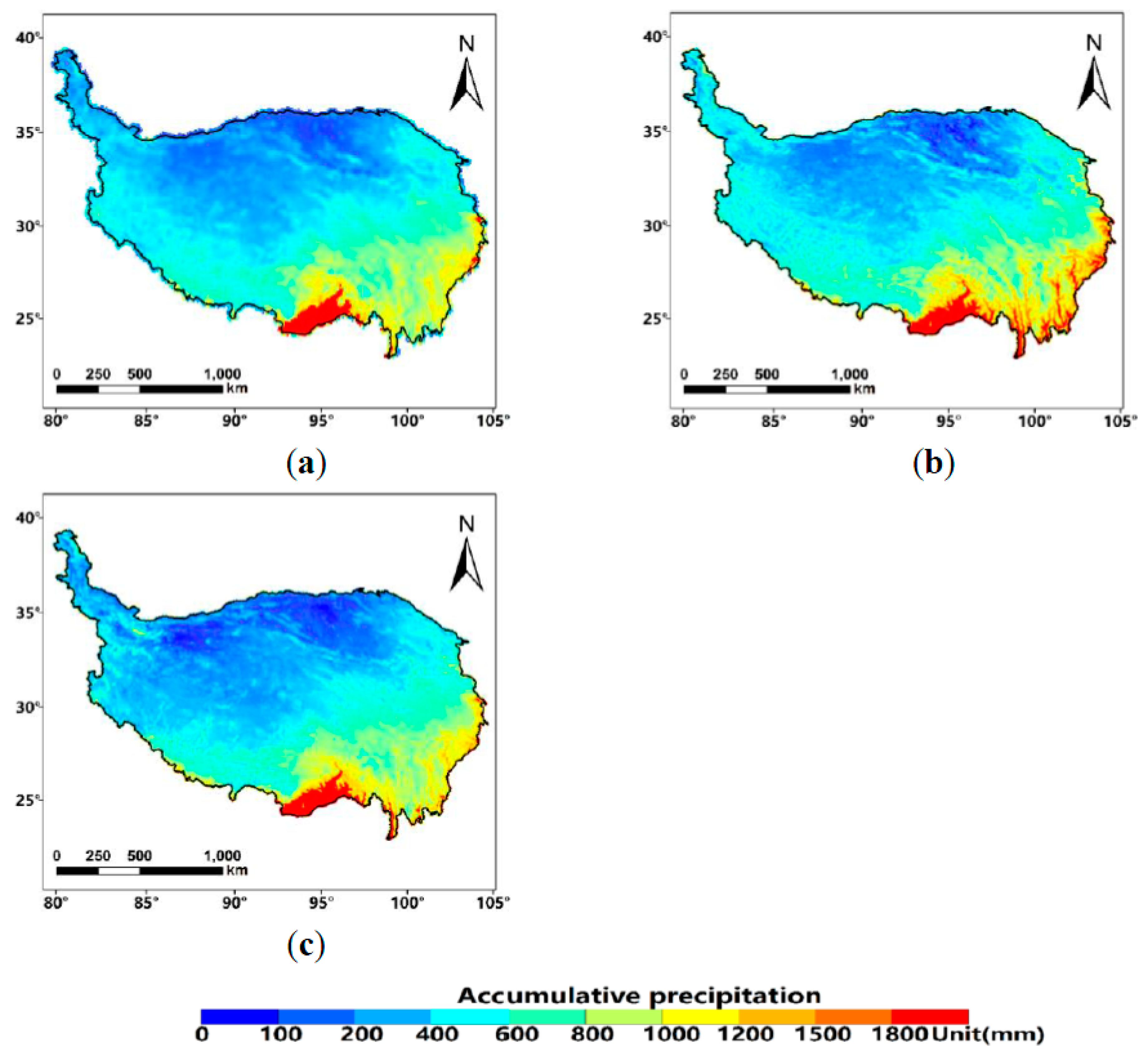
The annual downscaled results at 1 km resolution using random forest models based on TMPA and IMERG data were presented in Figure 9b,c, respectively. We additionally obtained the downscaled results at 0.1° based on TMPA which was displayed in Figure 9a. Both the downscaled results based on TMPA and IMERG captured the spatial distribution of annual precipitation compared to the original TMPA, original IMERG and gauge precipitation, showing a decreasing trend from south to north, and from west to east. It was notable that the downscaled results based TMPA data shown contiguous precipitation map with anomalies removed which appeared in the original TMPA data, in western and northern parts of the TP. The downscaled results based on IMERG data still displayed continuous variation and gradual trend without outliers.
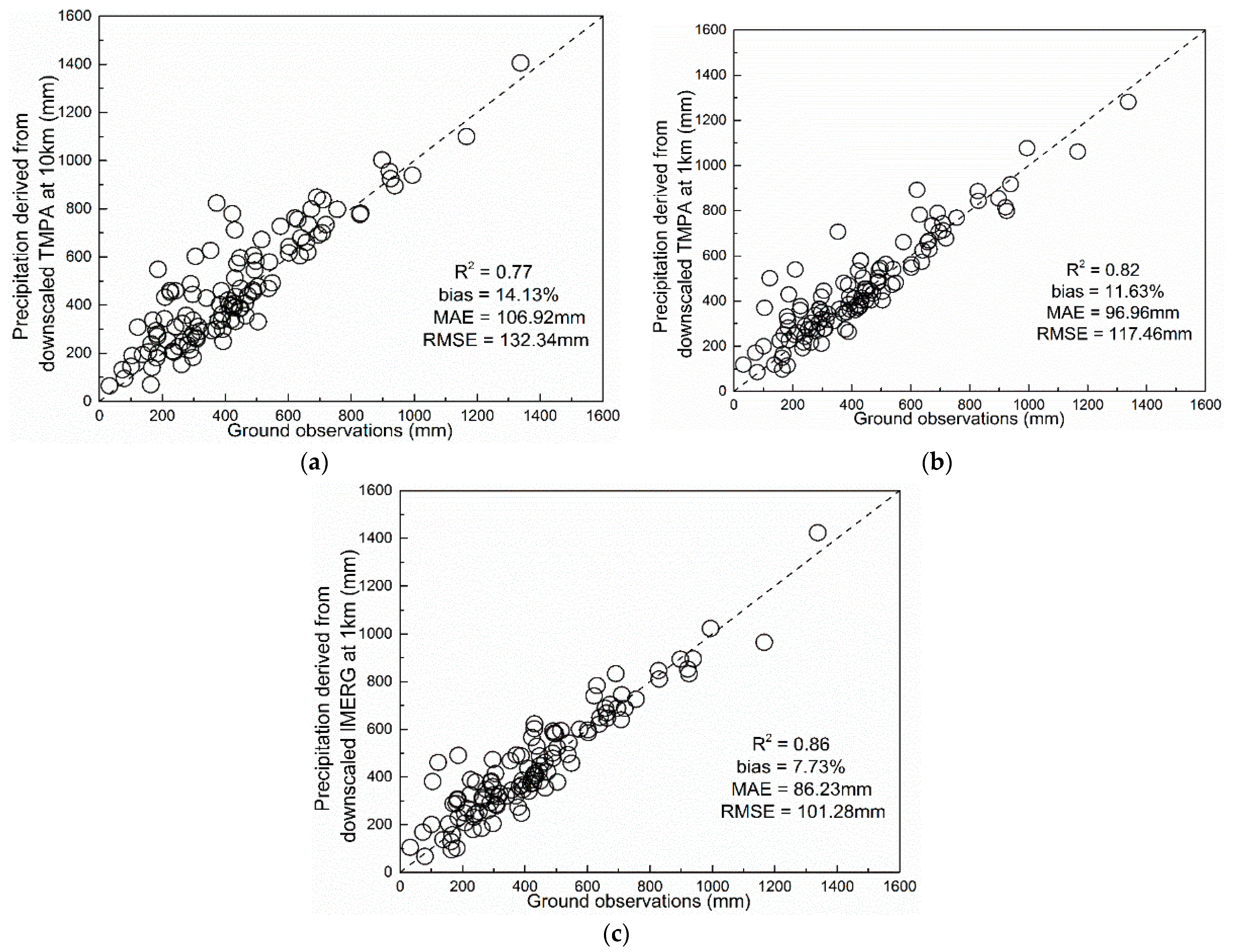
The performances of the downscaled results were validated against ground observations. Both the downscaled results still overestimated precipitation compared to ground observations but in lower degrees with reduced positive bias. The values of MAE and RMSE also decreased and R2 values increased in the downscaled results compared with the corresponding satellite products indicating the improved accuracy of downscaled results. Figure 10a shown the validation of the downscaled results based on TMPA data at 10 km resolution, while Figure 10b,c shown the validations of the downscaled results based on TMPA and IMERG data at 1 km, respectively, against ground observations. The downscaled results based on IMERG at 1 km had the best performance (R2 ~ 0.86, bias ~ 7.73%) among the three downscaled results based on TMPA and IMERG data and shown improved accuracy compared with the original IEMRG data (R2 ~ 0.74, bias ~ 12.23%). The downscaled results based on TMPA at 10 km and at 1 km also shown improvements compared with the original TMPA data (R2 ~ 0.67, bias ~ 22.40%), while the downscaled results based on TMPA at 1 km (R2 ~ 0.82, bias ~ 11.63%) performed better that the downscaled results at 10 km resolution based on TMPA data (R2 ~ 0.77, bias ~ 14.13%). Regrading to the comparison between the original IMERG data and the downscaled results based on TMPA at 10 km resolution, their performances were remarkably close compared to ground observations with R2 ~ 0.75 and bias ~ 13%.
Based on the disaggregation algorithm introduced in Section 3.3, the monthly downscaled results based on TMPA and IMERG were obtained. Table 2 presented the statistical results at monthly scale. The downscale results based on IMERG at 1 km shown the best accuracy at monthly scale with R2 ~ 0.82 and bias ~ 7% during wet seasons and R2 ~ 0.62 and bias ~ 10% during dry seasons. The downscaled results based on TMPA at 1 km also corresponded well with ground observations during wet seasons (R2 ~ 0.79 and bias ~ 10%) and shown relatively poorer performance during dry seasons (R2 ~ 0.58 and bias ~ 15%). Regrading to the downscaled results based on TMPA at 10 km resolution, the performance was equivalent to the original IMERG data at 10 km but better than the original TMPA data at . Generally, the accuracy of the downscaled results based on TMPA and IMERG performed better than those of the original satellite-based precipitation products, in each month.
4. Discussion
4.1. Anomalies in the Inland Water Bodies in TP
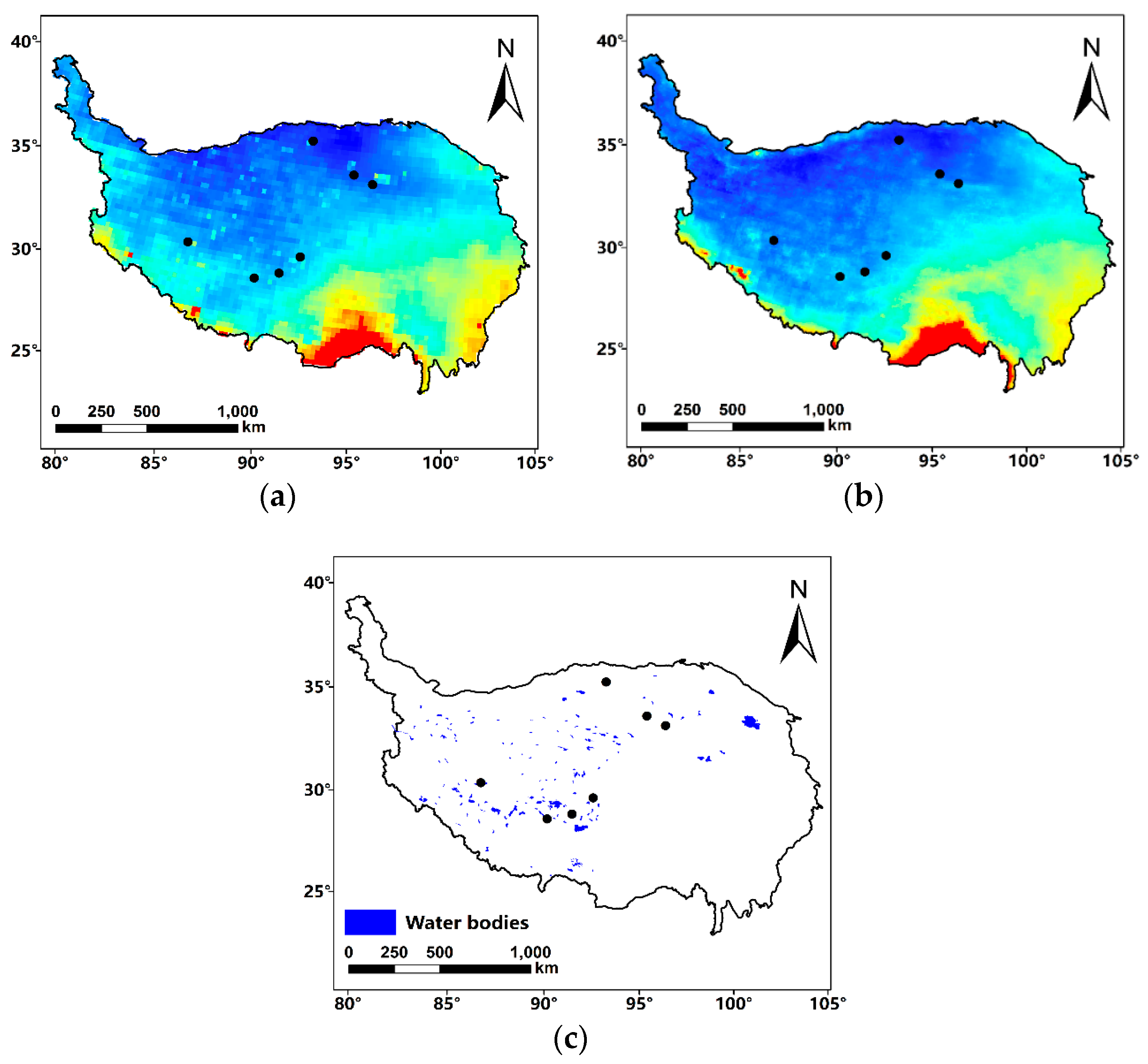
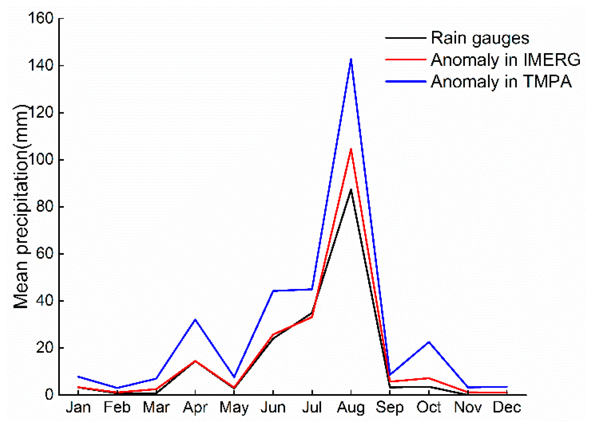
Systematic anomalies were observed in the western and northern part of the TP in the original TMPA 3B43 data. The phenomena were also found in [25,48,49]. They concluded that the systematic anomalies on the TP interior in satellite-based precipitation estimates were mainly affected by some water bodies. The distribution of inland water bodies was shown in Figure 11c. It was obtained from the Global Lakes and Wetlands Database (GLWD) (downloaded from: https://www.worldwildlife.org/publications/global-lakes-and-wetlands-database-large-lake-polygons-level-1). The spatial distributions of systematic anomalies were very close to those of inland water bodies. We further investigated the precipitation estimates covered by anomalies compared with rain gauges or its neighbors. Sites for seven anomalies which were located near water bodies were analyzed, as shown in Figure 12.
It was obvious that TMPA data tended to overestimate precipitation over inland water bodies, with mean bias ~ 78%. In contrast, IMERG data agreed quite well with ground observations (bias ~ 10%). The PMW retrievals might be the main source of the anomalies, and the deficiencies of PMW retrievals in the TMPA products (GPROF2010) led to the systematic overestimation. While IMERG employed the latest version of Goddard Profiling Algorithm (GPROF2014) to compute precipitation estimates from all PMW sensors onboard GPM satellites, it provided more consistent precipitation estimates over water bodies. For GPROF 2014, the surface type was classified based on the monthly emissivity for all SSM/I frequencies. The inland water bodies were treated as independent classes and were trained in the Bayes’ model, which was beneficial for estimating precipitation over water bodies. Thus, the unified and updated PMW algorithms used in IMERG products result in improved precipitation estimates over water bodies compared to TMPA products. Another possible reason for the improvement in the precipitation estimates over water bodies was that IMERG used GMI, which had a much better resolution than TMI equipped in TRMM, thus it can better identify the inland water bodies.
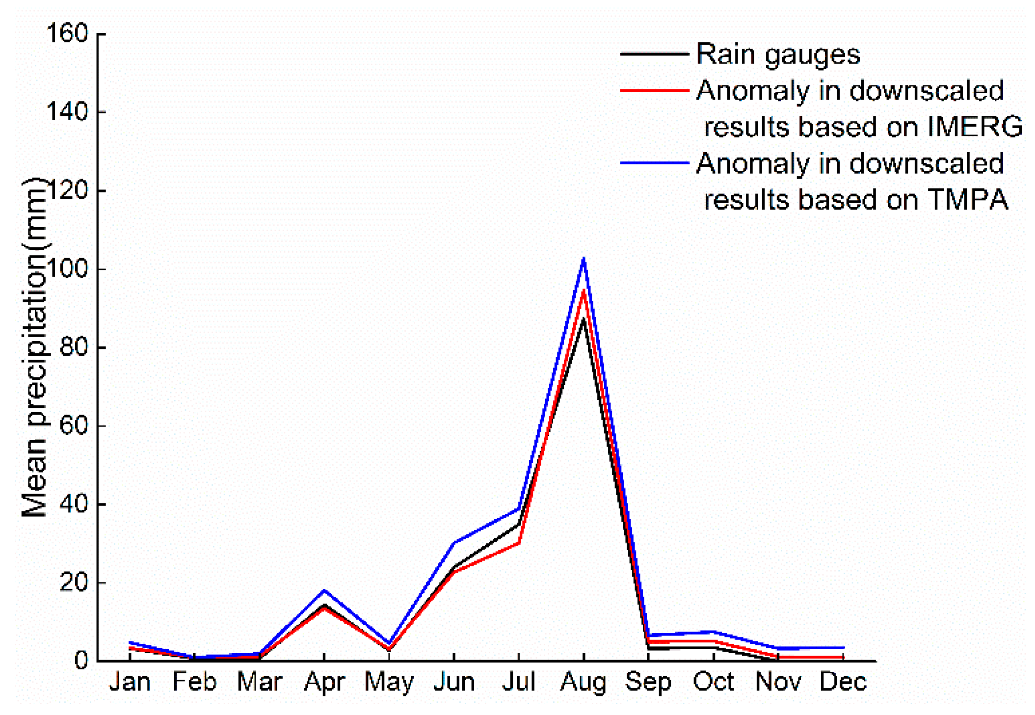
For the monthly downscaled results based on TMPA data and IMERG data using random forest algorithm and monthly disaggregation algorithm, we also calculated the precipitation estimates for the same seven sites for anomalies. The results were shown in Figure 13. Both the downscaled results based on TMPA data and IMERG data at 1 km resolution corresponded well with rain gauges. The bias was ~12% and 8% for the downscaled results based on TMPA and the downscaled results based on IMERG, respectively. The downscaled results based on TMPA and IMERG also eliminated the anomalies indicate that random forest was an effective way to improve the spatial resolutions with reasonable accuracy with systematic anomalies removed.
4.2. The Relationships between the Spatial Resolutions and the Accuracies of the Precipitation Estimates against Ground Observations
Though the accuracy of the precipitation estimates improved with the finer spatial resolutions, based on the statistical results presented in Table 1 and Table 2 in this study, it did not mean that the finer the spatial resolution, the better the precision. While in [50], the performances of the satellite-based precipitation products were better with decreasing spatial resolutions, in Lower Colorado River Basin (LCRB). The relationships between the spatial resolutions and the accuracies of satellite-based products might be affected by the density of rain gauge networks. For instance, over regions like LCRB, there were dense rain gauge networks, which enabled it possible to conduct the detailed assessment of the performances of the IMERG products at various resolutions. While in TP, there are sparsely and poorly constructed rain gauge networks, which made it not suitable to do researches exploring the relationships between spatial resolutions and the accuracies of remote sensing products. Generally, to compare the difference between point-based measurements (from rain gauges) and gridded estimates, the precipitation estimates from gauges located in the same pixel should be averaged, and then compared with the corresponding pixel values. More gauges would be contained in one pixel after upscaling, and thus the estimate errors at each gauge might be neutralized or alleviated. This might be one of the possible reasons to explain why the performances of remote sensing products improved after spatial resolution degradation. Further studies should be conducted to investigate the relationships between the spatial resolutions and the accuracies of satellite-based products, especially over regions where gauge network is coarse.
4.3. Future Research
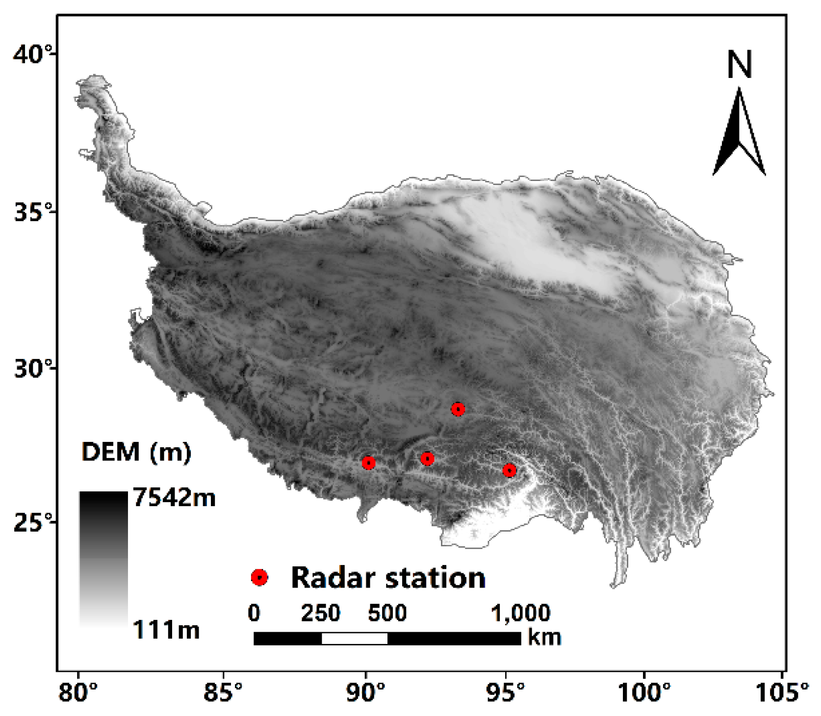
In this study, the precipitation measured by rain gauges were used to evaluate the performances of the original TMPA and IMERG data, as well as the downscaled results based on satellite-based precipitation products. However, due to the harsh environment and complex terrain, the rain gauges were sparsely and unevenly distributed over the TP. A majority of the gauges were located in north and east and at middle or low altitudes, while few gauges in the western part of the TP and at high elevations [51]. Thus, the assessment may not be representative and reasonable in the ungauged areas in western part of the TP and regions with high elevations. Though radar precipitation data is also widely used as ‘ground truth’ values to evaluate the quality of satellite-based precipitation data, radar networks are unsound over the TP. So far, there are only four working radar stations, shown in Figure 14. Additionally, other shortages, such as beam blockage and range degradation, cause radar precipitation merely useless over the TP. Therefore, more reliable ground reference data are highly needed for the TP.
Above all, this study evaluated the performances of TMPA and IMERG, and compared the downscaled results based on TMPA and IMERG, respectively, at annual and monthly temporal scales. However, the performance of satellite-based precipitation products may vary under extreme rainfall conditions, occurring at meteorological scale (e.g., hourly scale) [52]. It is very important to obtain the precipitation estimates with both finer spatial resolutions and accuracies to capture the extreme rainfall events, which is meaningful in flood disaster prevention. Therefore, additional downscaling techniques should be developed especially for higher temporal scales (hourly or half-hourly), to improve our understanding of precipitation activities during extreme rainfall events.
5. Conclusions
In this study, we focused on downscaling TMPA and IMERG data to generate precipitation estimates with a finer spatial resolution (~1 km) at annual scale, and a disaggregation algorithm was applied to obtain the monthly downscaled results based on those at annual scale. Both of the original satellite-based precipitation products (TMPA and IMERG) and the downscaled results were evaluated against ground observations. The main conclusions from this study were as follows:
- (1)
- The IMERG data provided more accurate precipitation estimates than TMPA data at both the annual and monthly scales. What’s more, compared with TMPA data, IMERG data did not have systematic anomalies any more.
- (2)
- The RF algorithm demonstrated potentials in downscaling TMPA and IMERG to obtain precipitation estimates with improved spatial resolution and reasonable accuracy over TP.
- (3)
- The downscaled results based on IMERG exhibited better performance than those based on TMPA data at both the annual and monthly scales.
Precipitation data with both fine spatial resolution and accuracy is highly needed in related fields. While precipitation data only with finer resolutions but low accuracy is, to some extent, useless, and vice versa. IMERG data indicated great potentials for researchers to obtain precipitation estimates with finer spatial resolutions and better accuracy worldwide. Additionally, after this study, we also found that the RF algorithm could serve as an alternative approach to improve both the spatial resolutions and accuracy of the coarse satellite-based products.
Author Contributions
Conceptualization, Z.M., K.H. and Y.H.; methodology, Z.M., K.H. and J.X.; software, J.X., X.T. and W.F.; validation, J.X., X.T., W.F., Y.H.; formal analysis, Z.M., K.H, J.X., X.T. and W.F.; investigation, Z.M., K.H, J.X., X.T., W.F. and Y.H.; resources, J.X., X.T., W.F. and Y.H.; data curation, K.H, J.X., X.T., W.F. and Y.H.; writing—original draft preparation, Z.M., K.H. and X.T.; writing—review and editing, Z.M., K.H, J.X., X.T., W.F., Y.H. and Y.H.; visualization, K.H, J.X., X.T., W.F. and Y.H.; supervision, Z.M., Y.H.; project administration, Z.M., Y.H.; funding acquisition, Z.M., Y.H.
Funding
This study was financially supported by the NSFC (Grant Nos. 91437214, 71461010701 and 41471430) and MOST Key-Project (Grant No. 2013CB036406) and China Postdoctoral Science Foundation (No. 2018M630037).
Acknowledgments
The authors would like to appreciate the NASA Precipitation Measurement Missions (PMM), the Level-1 and Atmosphere Archive & Distribution System (LAADS) Distributed Active Archive Center (DAAC), the Land Process (LP) Distributed Active Archive Center (DAAC) and the CGIAR Consortium for Spatial Information (CSI) for making the datasets available and the Third Pole Environment Database (TPE) for providing us with the gauge data for our areas of interests.
Conflicts of Interest
The authors declare no conflict of interest.
References
- Kidd, C.; Huffman, G. Global Precipitation Measurement. Meteorol. Appl. 2011, 18, 334–353. [Google Scholar] [CrossRef]
- Hou, A.Y.; Kakar, R.K.; Neeck, S.; Azarbarzin, A.A.; Kummerow, C.D.; Kojima, M.; Oki, R.; Nakamura, K.; Iguchi, T. The Global Precipitation Measurement Mission. Bull. Am. Meteorol. Soc. 2014, 95, 701–722. [Google Scholar] [CrossRef] [Green Version]
- Li, Z.; Yang, D.; Hong, Y. Multi-Scale Evaluation of High-Resolution Multi-Sensor Blended Global Precipitation Products over the Yangtze River. J. Hydrol. 2013, 500, 157–169. [Google Scholar] [CrossRef]
- Javanmard, S.; Yatagai, A.; Kawamoto, H.; Nodzu, M.; Jamali, J. Comparing High-Resolution Daily Gridded Precipitation Data with Satellite Rainfall Estimates of TRMM_3b42 over Iran. Adv. Geosci. 2010, 25, 119–125. [Google Scholar] [CrossRef] [Green Version]
- Villarini, G.; Krajewski, W.F. Review of the Different Sources of Uncertainty in Single Polarization Radar-Based Estimates of Rainfall. Surv. Geophys. 2009, 31, 107–129. [Google Scholar] [CrossRef]
- Huffman, G.J.; Adler, R.F.; Arkin, P.; Chang, A.; Ferraro, R.; Gruber, A.; Janowiak, J.; Mcnab, A.; Rudolf, B.; Schneider, U. The Global Precipitation Climatology Project (GPCP) Combined Precipitation Dataset. Bull. Am. Meteorol. Soc. 1997, 78, 5–20. [Google Scholar] [CrossRef] [Green Version]
- Huffman, G.J.; Adler, R.F.; Morrissey, M.M.; Bolvin, D.T.; Curtis, S.; Joyce, R.; Mcgavock, B.; Susskind, J. Global Precipitation at One-Degree Daily Resolution from Multisatellite Observations. J. Hydrometeorol. 2001, 2, 36–50. [Google Scholar] [CrossRef] [Green Version]
- Huffman, G.J.; Adler, R.F.; Bolvin, D.T.; Gu, G. Improving the global precipitation record: GPCP version 2.1. Geophys. Res. Lett. 2009, 36, 153–159. [Google Scholar] [CrossRef]
- Kubota, T.; Shige, S.; Hashizume, H.; Aonashi, K.; Takahashi, N.; Seto, S.; Hirose, M. Global Precipitation Map Using Satellite-Borne Microwave Radiometers by the Gsmap Project: Production and Validation. IEEE Trans. Geosci. Remote Sens. 2007, 45, 2259–2275. [Google Scholar] [CrossRef]
- Kummerow, C.; Simpson, J.; Thiele, O.; Barnes, W.; Chang, A.T.C.; Stocker, E.; Adler, R.F. The Status of the Tropical Rainfall Measuring Mission (TRMM) after Two Years in Orbit. J. Appl. Meteorol. 2000, 39, 1965–1982. [Google Scholar] [CrossRef] [Green Version]
- Kummerow, C.; Barnes, W.; Kozu, T.; Shiue, J.; Simpson, J. The Tropical Rainfall Measuring Mission (TRMM) Sensor Package. J. Atmos. Ocean. Technol. 1998, 15, 809–817. [Google Scholar] [CrossRef]
- Huffman, G.J.; Bolvin, D.T.; Nelkin, E.J.; Wolff, D.B.; Adler, R.F.; Gu, G.; Hong, Y.; Bowman, K.P.; Stocker, E.F. The TRMM Multisatellite Precipitation Analysis (TMPA): Quasi-Global, Multiyear, Combined-Sensor Precipitation Estimates at Fine Scales. J. Hydrometeorol. 2007, 8, 38–55. [Google Scholar] [CrossRef]
- Li, X.H.; Zhang, Q.; Xu, C.Y. Suitability of the TRMM Satellite Rainfalls in Driving a Distributed Hydrological Model for Water Balance Computations in Xinjiang Catchment, Poyang Lake Basin. J. Hydrol. 2012, 426–427, 28–38. [Google Scholar] [CrossRef]
- Li, L.; Hong, Y.; Wang, J.; Adler, R.F.; Policelli, F.S.; Habib, S.; Irwn, D.; Korme, T.; Okello, L. Evaluation of the Real-Time TRMM-Based Multi-Satellite Precipitation Analysis for an Operational Flood Prediction System in Nzoia Basin, Lake Victoria, Africa. Nat. Hazards 2009, 50, 109–123. [Google Scholar] [CrossRef]
- Islam, M.; Uyeda, H. Use of TRMM in Determining the Climatic Characteristics of Rainfall over Bangladesh. Remote Sens. Environ. 2007, 108, 264–276. [Google Scholar] [CrossRef]
- Huffman, G.J.; Bolvin, D.T.; Braithwaite, D.; Hsu, K.; Joyce, R.; Xie, P.P. GPM Integrated Multi-Satellite Retrievals for GPM (IMERG) Algorithm Theoretical Basis Document (Atbd) Version 4.4; PPS, NASA/GSFC: Washington, DC, USA, 2014; Volume 30.
- Tang, G.; Ma, Y.; Long, D.; Zhong, L.; Hong, Y. Evaluation of GPM Day-1 IMERG and TMPA Version-7 Legacy Products over Mainland China at Multiple Spatiotemporal Scales. J. Hydrol. 2016, 533, 152–167. [Google Scholar] [CrossRef]
- Prakash, S.; Mitra, A.K.; Aghakouchak, A.; Liu, Z.; Norouzi, H.; Pai, D.S. A Preliminary Assessment of GPM-Based Multi-Satellite Precipitation Estimates over a Monsoon Dominated Region. J. Hydrol. 2016, 556, 865–876. [Google Scholar] [CrossRef]
- Kim, K.; Park, J.; Baik, J.; Choi, M. Evaluation of Topographical and Seasonal Feature Using GPM IMERG and TRMM 3b42 over Far-East Asia. Atmos. Res. 2017, 187, 95–105. [Google Scholar] [CrossRef]
- Immerzeel, W.W.; Rutten, M.M.; Droogers, P. Spatial downscaling of TRMM precipitation using vegetative response on the Iberian Peninsula. Remote Sens. Environ. 2009, 113, 362–370. [Google Scholar] [CrossRef]
- Jia, S.; Zhu, W.; Lű, A.; Yan, T. A Statistical Spatial Downscaling Algorithm of TRMM Precipitation Based on NDVI and DEM in the Qaidam Basin of China. Remote Sens. Environ. 2011, 115, 3069–3079. [Google Scholar] [CrossRef]
- Teng, H.; Shi, Z.; Ma, Z.; Li, Y. Estimating Spatially Downscaled Rainfall by Regression Kriging Using TRMM Precipitation and Elevation in Zhejiang Province, Southeast China. Int. J. Remote Sens. 2014, 35, 7775–7794. [Google Scholar] [CrossRef]
- Xu, S.; Wu, C.; Wang, L.; Gonsamo, A.; Shen, Y.; Niu, Z. A new satellite-based monthly precipitation downscaling algorithm with non-stationary relationship between precipitation and land surface characteristics. Remote Sens. Environ. 2015, 162, 119–140. [Google Scholar] [CrossRef]
- Ma, Z.; Zhou, Y.; Hu, B.; Liang, Z.; Shi, Z. Downscaling Annual Precipitation with TMPA and Land Surface Characteristics in China. Int. J. Climatol. 2017, 37, 5107–5119. [Google Scholar] [CrossRef]
- Ma, Z.; Shi, Z.; Zhou, Y.; Xu, J.; Yu, W.; Yang, Y. A Spatial Data Mining Algorithm for Downscaling TMPA 3B43 V7 Data over the Qinghai–Tibet Plateau with the Effects of Systematic Anomalies Removed. Remote Sens. Environ. 2017, 200, 378–395. [Google Scholar] [CrossRef]
- Guo, Z.H.; Liu, X.M.; Xiao, W.F.; Wang, J.L.; Meng, C. Regionalization and Integrated Assessment of Climate Resource in China Based on GIS. Resour. Sci. 2007, 29, 2–9. [Google Scholar]
- Lin, Z.; Zhao, X. Spatial Characteristics of Changes in Temperature and Precipitation of the Qinghai-Xizang (Tibet) Plateau. Sci. China Ser. D Earth Sci. 1996, 39, 442–448. [Google Scholar]
- Yao, T.; Thompson, L.; Yang, W.; Yu, W.; Gao, Y.; Guo, X.; Yang, X. Different Glacier Status with Atmospheric Circulations in Tibetan Plateau and Surroundings. Nat. Clim. Change 2012, 2, 663–667. [Google Scholar] [CrossRef]
- Immerzeel, W.W.; Van Beek, L.P.; Bierkens, M.F. Climate change will affect the Asian water towers. Science 2010, 328, 1382–1385. [Google Scholar] [CrossRef] [PubMed]
- Huffman, G.J.; Bolvin, D.T.; Nelkin, E.J. Integrated Multi-satellitE Retrievals for GPM (IMERG) technical documentation. NASA/GSFC Code 2015, 612, 47. [Google Scholar]
- Xiao, J.F.; Moody, A. Trends in vegetation activity and their climatic correlates: China 1982 to 1998. Int. J. Remote Sens. 2004, 25, 5669–5689. [Google Scholar] [CrossRef]
- Evans, K.L.; James, N.A.; Gaston, K.J. Abundance, species richness and energy availability in the north American avifauna. Global Ecol. Biogeogr. 2006, 15, 372–385. [Google Scholar] [CrossRef]
- Grist, J.; Nicholson, S.E.; Mpolokang, A. On the Use of NDVI for Estimating Rainfall Fields in the Kalahari of Botswana. J. Arid Environ. 1997, 35, 195–214. [Google Scholar] [CrossRef]
- Iwasaki, H. NDVI Prediction over Mongolian Grassland Using GSMAP Precipitation Data and JRA-25/JCDAS Temperature Data. J. Arid Environ. 2009, 73, 557–562. [Google Scholar] [CrossRef]
- Warren, S.D.; Hohmann, M.G.; Auerswald, K.; Mitasova, H. An Evaluation of Methods to Determine Slope Using Digital Elevation Data. Catena 2004, 58, 215–233. [Google Scholar] [CrossRef]
- Xiong, J.; Zhang, J. Comparative Analysis of the Algorithms of Aspect Deriving from DEM-Take the Study of Loess Hill and Gully Area as the Case. Remote Sens. Inf. 2007, 22, 53–57. [Google Scholar]
- Chen, S.; Hong, Y.; Cao, Q.; Gourley, J.J.; Kirstetter, P.-E.; Yong, B.; Tian, Y. Similarity and Difference of the Two Successive V6 and V7 TRMM Multisatellite Precipitation Analysis Performance over China. J. Geophys. Res. Atmos. 2013, 118, 13,060–13,074. [Google Scholar] [CrossRef]
- Ruiz-Arias, J.A.; Tovar-Pescador, J.; Pozo-Vázquez, D.; Alsamamra, H. A Comparative Analysis of Dem-Based Models to Estimate the Solar Radiation in Mountainous Terrain. Int. J. Geogr. Inf. Sci. 2009, 23, 1049–1076. [Google Scholar] [CrossRef]
- Zhang, H.M.; Yang, Q.K.; Liu, Q.R.; Guo, W.L.; Wang, C.M. Regional Slope Length and Slope Steepness Factor Extraction Algorithm Based on GIS. Comput. Eng. 2010, 36, 246–248. [Google Scholar]
- Sørensen, R.; Seibert, J. Effects of Dem Resolution on the Calculation of Topographical Indices: TWI and its Components. J. Hydrol. 2007, 347, 79–89. [Google Scholar] [CrossRef]
- Gallant, J.C.; Dowling, T.I. A Multiresolution Index of Valley Bottom Flatness for Mapping Depositional Areas. Water Resour. Res. 2003, 39, 1347. [Google Scholar] [CrossRef]
- Mukherjee, S.; Mukherjee, S.; Garg, R.D.; Bhardwaj, A.; Raju, P.L.N. Evaluation of Topographic Index in Relation to Terrain Roughness and Dem Grid Spacing. J. Earth Syst. Sci. 2013, 122, 869–886. [Google Scholar] [CrossRef]
- Breiman, L. Random Forests. Mach. Learn. 2001, 45, 5–32. [Google Scholar] [CrossRef] [Green Version]
- Breiman, L.; Friedman, J.; Stone, C.J.; Olshen, R.A. Classification and Regression Trees; Wadsworth: Belmont, CA, USA, 1984. [Google Scholar]
- Cutler, A.; Cutler, D.R.; Stevens, J.R. Random Forests. In Ensemble Machine Learning; Zhang, C., Ma, Y., Eds.; Springer: Boston, MA, USA, 2012; pp. 157–175. [Google Scholar]
- Immerzeel, W.W.; Quiroz, R.A.; De Jong, S.M. Understanding Precipitation Patterns and Land Use Interaction in Tibet Using Harmonic Analysis of SPOT VGT-S10 NDVI Time Series. Int. J. Remote Sens. 2005, 26, 2281–2296. [Google Scholar] [CrossRef]
- Duan, Z.; Bastiaanssen, W.G.M. First Results from Version 7 TRMM 3B43 Precipitation Product in Combination with a New Downscaling–Calibration Procedure. Remote Sens. Environ. 2013, 131, 1–13. [Google Scholar] [CrossRef]
- Tang, G.; Long, D.; Hong, Y. Systematic Anomalies over Inland Water Bodies of High Mountain Asia in TRMM Precipitation Estimates: No Longer a Problem for the GPM Era? IEEE Geosci. Remote Sens. Lett. 2016, 13, 1762–1766. [Google Scholar] [CrossRef]
- Ma, Z.Q.; Zhou, L.Q.; Yu, W.; Yang, Y.Y.; Teng, H.F.; Shi, Z. Improving TMPA 3B43 V7 Data Sets Using Land-Surface Characteristics and Ground Observations on the Qinghai–Tibet Plateau. IEEE Geosci. Remote Sens. Lett. 2018, 99, 1–5. [Google Scholar] [CrossRef]
- Omranian, E.; Sharif, H.O. Evaluation of the Global Precipitation Measurement (GPM) satellite rainfall products over the Lower Colorado River Basin, Texas. J. Am. Water Resour. Assoc. 2018, 54, 882–898. [Google Scholar] [CrossRef]
- Ma, Z.Q.; Xu, Y.P.; Peng, J.; Chen, Q.X.; Wan, D.; He, K.; Shi, Z.; Li, H.Y. Spatial and temporal precipitation patterns characterized by TRMM TMPA over the Qinghai-Tibetan plateau and surroundings. Int. J. Remote Sens. 2018, 38, 3891–3907. [Google Scholar] [CrossRef]
- Omranian, E.; Sharif, H.O. How Well Can Global Precipitation Measurement (GPM) Capture Hurricanes? Case Study: Hurricane Harvey. Remote Sens. 2018, 10, 1150. [Google Scholar] [CrossRef]
Figure 1.
Spatial distribution of gauge stations and the Digital Elevation Model (DEM) over the Tibetan Plateau (TP).
Figure 1.
Spatial distribution of gauge stations and the Digital Elevation Model (DEM) over the Tibetan Plateau (TP).

Figure 2.
The flow chart of the random forest-based downscaling algorithm used in the study.

Figure 3.
Spatial distribution of precipitation maps generated from (a) original TRMM Multisatellite Precipitation Analysis (TMPA) data (), (b) resampled IMERG data () and (c) original Integrated Multi-satellitE Retrievals for Global Precipitation Measurement (IMERG) data (), over the TP in 2015.
Figure 3.
Spatial distribution of precipitation maps generated from (a) original TRMM Multisatellite Precipitation Analysis (TMPA) data (), (b) resampled IMERG data () and (c) original Integrated Multi-satellitE Retrievals for Global Precipitation Measurement (IMERG) data (), over the TP in 2015.


Figure 4.
Scatterplots of the validation between ground observations and (a) the original TMPA data at a spatial resolution of ; (b) the resampled IMERG data at a spatial resolution of ; and (c) the original IMERG data at a spatial resolution of , at the annual scale.
Figure 4.
Scatterplots of the validation between ground observations and (a) the original TMPA data at a spatial resolution of ; (b) the resampled IMERG data at a spatial resolution of ; and (c) the original IMERG data at a spatial resolution of , at the annual scale.


Figure 5.
Monthly mean precipitation from 113 rain gauges (gray bar), the original TMPA (blue line), the resampled IMERG (green line) and the original IMERG (red line) for the TP from January to December 2015.
Figure 5.
Monthly mean precipitation from 113 rain gauges (gray bar), the original TMPA (blue line), the resampled IMERG (green line) and the original IMERG (red line) for the TP from January to December 2015.

Figure 6.
Graphs of the variation of the ‘out of bag’ (OOB) error rate for (a) and (b) at different ntree values. Note: OOB error denoted the ‘out of bag’ error provided by the bagging model. and denoted the random forest models based on TMPA data and IMERG data, respectively.
Figure 6.
Graphs of the variation of the ‘out of bag’ (OOB) error rate for (a) and (b) at different ntree values. Note: OOB error denoted the ‘out of bag’ error provided by the bagging model. and denoted the random forest models based on TMPA data and IMERG data, respectively.

Figure 7.
Boxplots of Variation of the OOB error rate for (a) and (b) at different values. Note: OOB error denoted the ‘out of bag’ error provided by the bagging model. and denoted the random forest models based on TMPA data and IMERG data, respectively.
Figure 7.
Boxplots of Variation of the OOB error rate for (a) and (b) at different values. Note: OOB error denoted the ‘out of bag’ error provided by the bagging model. and denoted the random forest models based on TMPA data and IMERG data, respectively.

Figure 8.
The order of variables’ importance in (a) and (b) . Note: and denoted the random forest models based on TMPA data and IMERG data, respectively.
Figure 8.
The order of variables’ importance in (a) and (b) . Note: and denoted the random forest models based on TMPA data and IMERG data, respectively.

Figure 9.
Spatial distribution of precipitation maps generated from (a) downscaled results based on TMPA data at 0.1°, (b) downscaled results based on TMPA data at 1 km and (c) downscaled results based on IMERG data at 1 km, over the TP in 2015.
Figure 9.
Spatial distribution of precipitation maps generated from (a) downscaled results based on TMPA data at 0.1°, (b) downscaled results based on TMPA data at 1 km and (c) downscaled results based on IMERG data at 1 km, over the TP in 2015.

Figure 10.
Scatterplots of the validation between ground observations and (a) downscaled results based on TMPA data at 10 km; (b) downscaled results based on TMPA data at 1 km and (c) downscaled results based on IMERG data at 1 km, at the annual scale.
Figure 10.
Scatterplots of the validation between ground observations and (a) downscaled results based on TMPA data at 10 km; (b) downscaled results based on TMPA data at 1 km and (c) downscaled results based on IMERG data at 1 km, at the annual scale.

Figure 11.
Spatial distribution of precipitation estimates generated from (a) TMPA 3b43, (b) IMERG Final and (c) inland water bodies from Global Lakes and Wetlands Database (GLWD). The black circles represent the sites for anomalies.
Figure 11.
Spatial distribution of precipitation estimates generated from (a) TMPA 3b43, (b) IMERG Final and (c) inland water bodies from Global Lakes and Wetlands Database (GLWD). The black circles represent the sites for anomalies.

Figure 12.
Comparison of mean monthly precipitation data for the anomalies covering inland water bodies in the original TMPA 3B43 data (blue line) and the original IMERG data (red line) with the data from seven rain gauge stations (black line).
Figure 12.
Comparison of mean monthly precipitation data for the anomalies covering inland water bodies in the original TMPA 3B43 data (blue line) and the original IMERG data (red line) with the data from seven rain gauge stations (black line).

Figure 13.
Comparison of mean monthly precipitation data of the anomalies covering inland water bodies in the downscaled results based on TMPA data (blue line) and the downscaled results based IMERG data (red line) with the data from seven rain gauge stations (black line).
Figure 13.
Comparison of mean monthly precipitation data of the anomalies covering inland water bodies in the downscaled results based on TMPA data (blue line) and the downscaled results based IMERG data (red line) with the data from seven rain gauge stations (black line).

Figure 14.
The spatial distribution of radar stations over the TP.


Table 1.
Coefficients of determination (R2), bias, mean absolute error (MAE) and root mean square error (RMSE) of the original TMPA data, the resampled IMERG data and the original IMERG data, compared with ground observations at each month in 2015.
Table 1.
Coefficients of determination (R2), bias, mean absolute error (MAE) and root mean square error (RMSE) of the original TMPA data, the resampled IMERG data and the original IMERG data, compared with ground observations at each month in 2015.
| Jan | Feb | Mar | Apr | May | Jun | Jul | Aug | Sep | Oct | Nov | Dec | ||
|---|---|---|---|---|---|---|---|---|---|---|---|---|---|
| Original TMPA | R2 | 0.57 | 0.56 | 0.48 | 0.51 | 0.53 | 0.67 | 0.68 | 0.67 | 0.74 | 0.48 | 0.37 | 0.39 |
| Bias (%) | 6.29 | 46.54 | 65.57 | 14.30 | 29.40 | 16.86 | 19.59 | 18.35 | 21.25 | 47.02 | 81.07 | 53.79 | |
| MAE (mm) | 4.20 | 4.18 | 7.98 | 14.75 | 20.19 | 27.45 | 22.53 | 31.45 | 23.98 | 10.71 | 3.75 | 2.20 | |
| RMSE (mm) | 10.21 | 6.55 | 14.48 | 22.42 | 28.00 | 37.89 | 32.01 | 50.42 | 31.06 | 15.41 | 5.64 | 3.53 | |
| Resampled IMERG | R2 | 0.56 | 0.66 | 0.67 | 0.63 | 0.69 | 0.74 | 0.71 | 0.68 | 0.75 | 0.56 | 0.58 | 0.42 |
| Bias (%) | −13.02 | 19.78 | 32.75 | −4.74 | 13.59 | 13.50 | 8.19 | 13.27 | 16.48 | 20.14 | 51.24 | 31.74 | |
| MAE (mm) | 3.43 | 3.02 | 5.50 | 12.10 | 15.35 | 23.20 | 18.30 | 27.97 | 21.00 | 8.32 | 2.65 | 1.87 | |
| RMSE (mm) | 9.96 | 5.00 | 9.84 | 19.60 | 19.79 | 30.67 | 27.30 | 42.45 | 28.00 | 11.27 | 3.50 | 3.20 | |
| Original IMERG | R2 | 0.55 | 0.69 | 0.58 | 0.59 | 0.72 | 0.74 | 0.72 | 0.67 | 0.74 | 0.62 | 0.57 | 0.48 |
| Bias (%) | −12.53 | 17.59 | 38.85 | −4.27 | 12.14 | 14.23 | 7.60 | 13.31 | 16.22 | 16.86 | 45.86 | 26.04 | |
| MAE(mm) | 3.56 | 3.13 | 5.96 | 12.45 | 14.43 | 23.61 | 17.79 | 27.86 | 22.15 | 7.59 | 2.54 | 1.85 | |
| RMSE(mm) | 10.10 | 5.32 | 12.97 | 20.72 | 18.70 | 31.25 | 26.47 | 43.01 | 28.22 | 10.62 | 3.43 | 3.59 |
Table 2.
Coefficients of determination (R2), bias, mean absolute error (MAE) and root mean square error (RMSE) for the downscaled results based on TMPA data at 10 km, the downscaled results based on TMPA data at 1 km and downscaled results based on IMERG data at 1 km, against ground observations at each month in 2015.
| Jan | Feb | Mar | Apr | May | Jun | Jul | Aug | Sep | Oct | Nov | Dec | ||
|---|---|---|---|---|---|---|---|---|---|---|---|---|---|
| Downscaled results | R2 | 0.57 | 0.60 | 0.57 | 0.59 | 0.68 | 0.80 | 0.75 | 0.70 | 0.76 | 0.52 | 0.58 | 0.42 |
| based on TMPA | Bias (%) | 12.23 | 20.54 | 25.67 | 14.30 | 10.40 | 16.86 | 19.59 | 11.35 | 11.25 | 7.02 | 21.23 | 13.79 |
| data at 10 km | MAE (mm) | 3.79 | 3.77 | 7.20 | 13.31 | 18.22 | 24.77 | 22.33 | 23.38 | 21.64 | 9.67 | 3.38 | 1.99 |
| RMSE (mm) | 9.70 | 6.22 | 13.76 | 21.30 | 26.60 | 36.00 | 30.41 | 37.90 | 29.51 | 14.64 | 5.36 | 3.35 | |
| Downscaled results | R2 | 0.58 | 0.68 | 0.63 | 0.63 | 0.79 | 0.82 | 0.81 | 0.77 | 0.79 | 0.68 | 0.60 | 0.46 |
| based on TMPA | Bias (%) | 10.76 | 14.93 | 22.75 | 13.23 | 7.45 | 11.27 | 13.44 | 7.26 | 11.96 | 6.48 | 20.23 | 8.47 |
| data at 1 km | MAE (mm) | 3.09 | 2.72 | 4.95 | 10.89 | 13.82 | 20.88 | 19.47 | 18.17 | 18.90 | 7.49 | 2.39 | 1.68 |
| RMSE (mm) | 8.96 | 5.50 | 8.86 | 17.64 | 17.81 | 27.60 | 24.57 | 28.21 | 25.20 | 10.14 | 3.15 | 2.88 | |
| Downscaled results | R2 | 0.60 | 0.74 | 0.64 | 0.61 | 0.80 | 0.85 | 0.81 | 0.79 | 0.82 | 0.68 | 0.63 | 0.51 |
| based on IMERG | Bias (%) | 8.12 | 6.47 | 14.76 | 3.38 | 2.56 | 7.29 | 8.63 | 4.11 | 8.42 | 4.48 | 14.87 | 6.72 |
| data at 10 km | MAE (mm) | 2.01 | 3.00 | 4.66 | 8.80 | 10.11 | 15.12 | 15.33 | 13.00 | 12.00 | 5.00 | 2.10 | 1.00 |
| RMSE (mm) | 7.50 | 4.78 | 8.32 | 14.32 | 16.77 | 20.21 | 19.56 | 22.00 | 18.32 | 9.09 | 3.06 | 2.71 |
© 2018 by the authors. Licensee MDPI, Basel, Switzerland. This article is an open access article distributed under the terms and conditions of the Creative Commons Attribution (CC BY) license (http://creativecommons.org/licenses/by/4.0/).
Share and Cite
MDPI and ACS Style
Ma, Z.; He, K.; Tan, X.; Xu, J.; Fang, W.; He, Y.; Hong, Y. Comparisons of Spatially Downscaling TMPA and IMERG over the Tibetan Plateau. Remote Sens. 2018, 10, 1883. https://doi.org/10.3390/rs10121883
AMA Style
Ma Z, He K, Tan X, Xu J, Fang W, He Y, Hong Y. Comparisons of Spatially Downscaling TMPA and IMERG over the Tibetan Plateau. Remote Sensing. 2018; 10(12):1883. https://doi.org/10.3390/rs10121883
Chicago/Turabian StyleMa, Ziqiang, Kang He, Xiao Tan, Jintao Xu, Weizhen Fang, Yu He, and Yang Hong. 2018. "Comparisons of Spatially Downscaling TMPA and IMERG over the Tibetan Plateau" Remote Sensing 10, no. 12: 1883. https://doi.org/10.3390/rs10121883
Note that from the first issue of 2016, this journal uses article numbers instead of page numbers. See further details here.