Article

Improved Albedo Estimates Implemented in the METRIC Model for Modeling Energy Balance Fluxes and Evapotranspiration over Agricultural and Natural Areas in the Brazilian Cerrado

1
Remote Sensing Division, National Institute for Space Research-INPE, São José dos Campos 12227-010, Brazil
2
Departamento de Ciencias Agrarias, Universidad Católica del Maule, Curicó 3341695, Chile
3
Department of Geography, University of São Paulo, São Paulo 05508-000, Brazil
*
Author to whom correspondence should be addressed.
Remote Sens. 2018, 10(8), 1181; https://doi.org/10.3390/rs10081181
Submission received: 4 April 2018 / Revised: 17 May 2018 / Accepted: 19 May 2018 / Published: 26 July 2018
(This article belongs to the Special Issue Remote Sensing Water Cycle: Theory, Sensors, Data, and Applications)

Abstract

:
In this study we assessed METRIC (Mapping Evapotranspiration at high Resolution with Internalized Calibration) model performance to estimate energy balance fluxes and evapotranspiration (ET) in two heterogeneous landscapes in the Brazilian Cerrado, including fluxes and ET in both agricultural and natural vegetation. The estimates were evaluated by comparing them to flux tower data collected over sugarcane (USR site), woody savanna (PDG site) and stricto-sensu savanna (RECOR site) areas. The selection of the study years (2005–2007 for USR/PDG sites and 2011–2015 for RECOR site) was based on the availability of meteorological data (to be used as inputs in METRIC) and of flux tower data for energy balance fluxes and ET comparisons. The broadband albedo submodel was adjusted in order to improve Net Radiation estimates. For this adjustment, we applied at-surface solar radiation simulations obtained from the SMARTS2 model under different conditions of land elevation, precipitable water content and solar angles. We also tested the equivalence between the measured crop coefficient (Kc_ec) and the reference evapotranspiration fraction (ETrF or F), seeking to extrapolate from instantaneous to daily values of actual evapotranspiration (ETa). Surface albedo was underestimated by 10% at the USR site (showing a better performance for full crop coverage), by 15% at the PDG site (following the woody savanna dynamics pattern through dry and wet seasons) and was overestimated by 21% at the RECOR site. METRIC was effective in simulating the spatial and temporal variability of energy balance fluxes and ET over agricultural and natural vegetation in the Brazilian Cerrado, with errors within those reported in the literature. Net radiation (Rn) presented consistent results (coefficient of determination (R2) > 0.94) but it was overestimated by 8% and 9% in sugarcane and woody savanna, respectively. METRIC-derived ET estimates showed an agreement with ground data at USR and PDG sites (R2 > 0.88, root mean square error (RMSE) up to 0.87 mm day−1), but at the RECOR site, ET was overestimated by 14% (R2 = 0.96, mean absolute error (MAE) = 0.62 mm.day−1 and RMSE = 0.75 mm day−1). Surface energy balance fluxes and ET were marked by seasonality, with direct dependence on available energy, rainfall distribution, soil moisture and other parameters like albedo and NDVI.

Graphical Abstract

1. Introduction

Brazilian tropical biomes, mainly represented by the Amazon rainforest and the Cerrado (Brazilian savanna), have been the focus of global attention due to their great biological diversity as well as the impact of deforestation on climate, hydrology, and biogeochemical cycles at regional and global scales [1]. The Brazilian Cerrado consists of complex vegetation which is ecologically and physiognomically related to other savannas in tropical America, Africa and Australia [2]. Its area includes much of central Brazil, part of northeastern Paraguay and eastern Bolivia, making it not only the second largest Brazilian biome (2,036,448 km2—approximately 24% of the national territory), but also one of the richest regions in terms of biodiversity on the planet [3]. Besides its importance for national agriculture, the Cerrado plays a vital role in the dynamics of water resources in Brazil, including parts of 12 hydrographic regions, in addition to housing some of the largest hydroelectric power plants in the country (accounting for 80% of Brazil’s national electrical energy production) [4].
This biome has been showing deforestation rates as high as those for the Amazon region, despite possessing an area that is half of its size. IBAMA’s Biome Monitoring and Deforestation Program estimated that in 2010 the deforested area in the Cerrado was 6469 km2, while in the Legal Amazon it was 7000 km2. Until 2010, the Cerrado’s deforested area corresponded to 47% of the biome total area, which demonstrates that in some of its central-south regions, native vegetation has almost disappeared altogether. In São Paulo State, more than 90% of the original Cerrado vegetation has been cleared, as opposed to 16.6% in Piauí State. The states with the largest converted areas are Goiás, Minas Gerais, and Mato Grosso do Sul [3,5,6]. For a long time this region was seen as inadequate for agriculture due to the low fertility of its soils, but advances in productive and technological systems, governmental incentives, favorable topographic conditions for mechanization, and low land prices have contributed to turning the Cerrado into a region of intense agricultural activity [7], especially for soybean, corn, sugarcane, beans, cotton, and coffee crops [2,8]. Thus, agricultural expansion in the Cerrado is the main reason why Brazilian agriculture occupies an internationally scrutinized position, with a biome that has been considered one of the main global hotspots in the expansion of agricultural crops in the last 50 years [9].
However, land cover and land use changes, triggered by the expansion of agricultural activities, promote the emission of greenhouse gases, causing impacts on water and energy balances [7,8,10], and have the potential to affect ecosystems and diverse economic sectors, such as energy production and water supply. Below average rainfall in some regions of Brazil already requires attention and the careful monitoring of production and food supply throughout the year. Combined with low precipitation, elevated temperatures increase evapotranspiration, which reduces water availability for agricultural crops. Therefore, in the current context of a water crisis, any attempt to improve water use efficiency should be based on reliable ET estimates, including evaporation of soil water or free surfaces and vegetation transpiration [11,12].
Evapotranspiration is the total amount of water transferred from soil, free surfaces, wet vegetation, and plant transpiration to the atmosphere. It is the second largest component of the water cycle (after precipitation), as it returns more than 60% of the precipitable water to the atmosphere, and uses more than half of the solar energy absorbed by the Earth’s surface [13,14,15], relating directly to energy, water availability and climate. In addition to its importance to the hydrological cycle, ET has a relevant participation in global climate dynamics and processes of the primary productivity of terrestrial ecosystems [16,17,18]. This variable is also related to land cover, as it is controlled by the available solar energy, aerodynamic conditions of the atmosphere, water availability in the soil, and by vegetation characteristics such as phenological stage, canopy geometry and structure/depth of the root system [19].
The spatial and temporal monitoring of ET represents a great challenge to the understanding of the energy and the hydrological partitioning between the surface and the atmosphere in different biomes, especially in tropical areas, where the largest sources of ET are located. In addition, accurate ET estimates are needed to model water resources, assess water balance, assist in irrigation management at the local and regional scale, and monitor water availability and consumption [1,20,21].
In agriculture, the actual crop ET (ETa) is traditionally calculated by multiplying the crop coefficient (Kc) by the reference evapotranspiration (ETr), estimated using field weather-based data and the Penman-Monteith (PM) equation [22,23]. ETa consists on the amount of water transferred to the atmosphere under the actual conditions of atmospheric demand, soil moisture, and crop conditions [24]. Reference ET is defined as the ET of an hypothetical reference surface, such as alfalfa (ETr) or grass (ETo), with a certain height and surface aerodynamic resistance, under well-watered conditions and representing an extension of at least 100 m with the same or similar vegetation [25]. This approach is widely used in agriculture because of its simplicity and low data requirements [26].
Other ways to accurately determine ET in situ are lysimeters and towers equipped with Bowen Ratio or eddy covariance (EC) systems [27]. These methods are widely used in many biomes, including deserts, savannas, pastures, forests, and agricultural areas, but they present a high cost of installation and maintenance. Another limitation of these methods is the impossibility of extending the analysis to large areas due to the heterogeneity of their surfaces and the dynamic nature of heat transfer processes [11,28,29]. In this sense, remote sensing has the advantage of allowing reliable estimations of spatialized ET for various types of vegetation cover, with low cost and adequate repeatability for monitoring agricultural crops [29]. Moreover, the continuous and spatialized quantification of surface physical parameters allows the improvement of agrometeorological models as well as weather and climate predictions [30].
Among the various models developed to estimate ET with remote sensing data, remote sensing energy balance (RSEB) models are currently considered to be the best method for monitoring water use in agricultural crops at local and regional scale [11,17,23,31], requiring surface reflectance and thermal images, as well as complementary surface data. METRIC (Mapping EvapoTranspiration with high Resolution and Internalized Calibration) [32] is a one-source model derived from the Surface Energy Balance (SEBAL) model [33] for applications in irrigated agricultural areas. METRIC utilizes ground-based ETr data acquired at a region of interest to inversely and internally calibrate surface energy balance, which facilitates determining the extreme conditions of heat exchange over agricultural areas (the anchor pixels), aiming to calibrate the sensible heat flux at the pixel-level [23].
Even though latent heat flux is calculated as the residual term of the energy balance, its accuracy depends on the quality of the modeling for other terms and biophysical parameters such as albedo, leaf area index, and momentum roughness length [23]. Thus, in this study we evaluated the potential of the METRIC model to estimate the energy balance fluxes and ET over heterogeneous Cerrado regions, and to represent the spatial and temporal pattern of ET in agriculture and natural land covers. To feed METRIC, we applied MODIS/Terra satellite products and surface meteorological data as input. To validate our estimates, measurements from three flux towers located at (i) a sugarcane field, (ii) a woody savanna and (iii) in a stricto-sensu area were employed. As an improvement in this study, we proposed a modification to the Net Radiation estimation by adjusting the broadband surface albedo submodel, using the SMARTS2 model [34] and the method applied by [35,36], which integrate band reflectances according to the intensities of at-surface incoming solar radiation within the domain of the band.

2. Materials and Methods
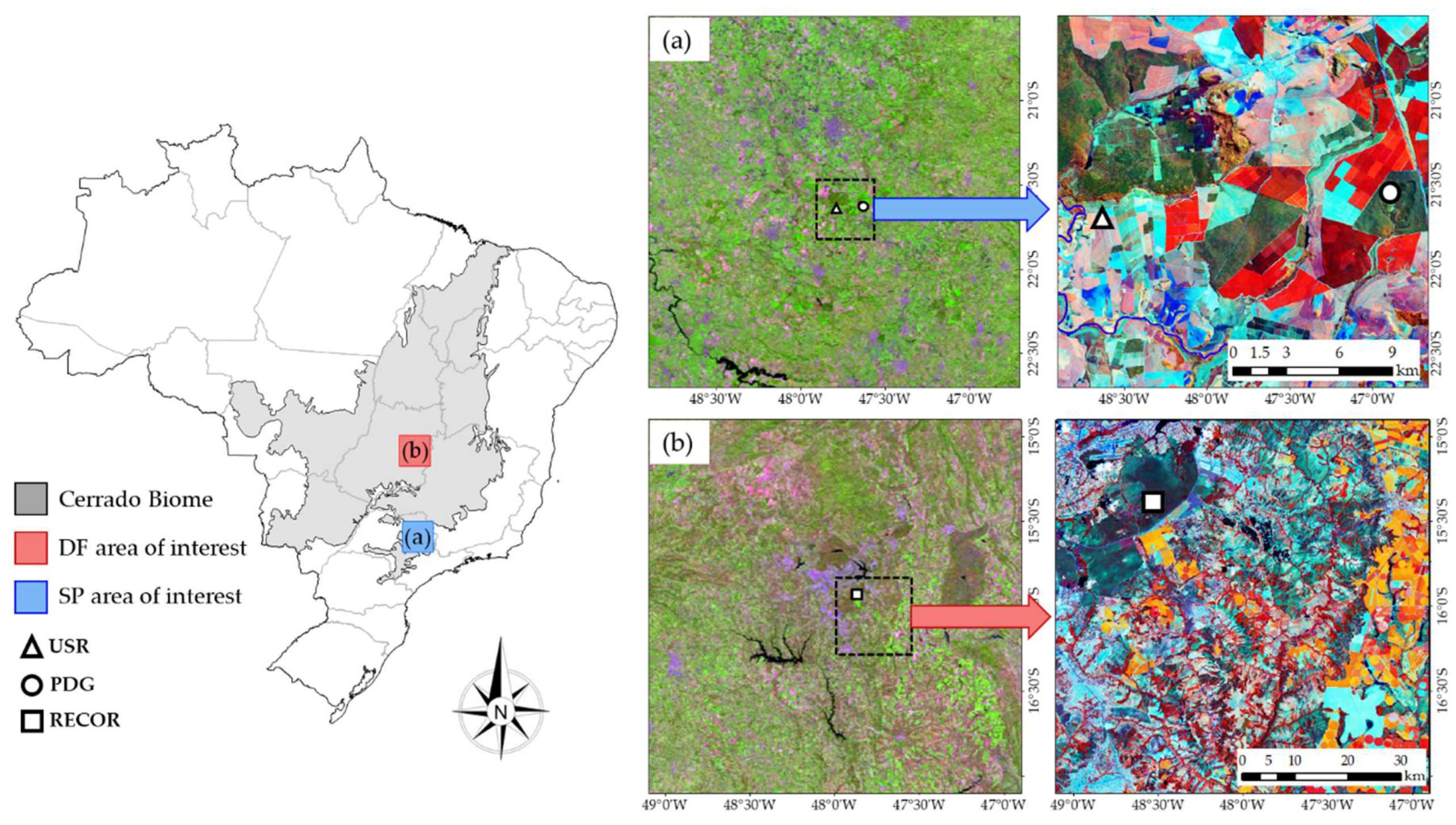
2.1. Study Area

This study was conducted for two heterogeneous areas of interest (AOIs) in the Brazilian Cerrado (Figure 1), with simultaneous presence of agriculture and natural vegetation. Each AOI evaluated consists of a 2° × 2° plot centralized in the position of the flux towers (described in Section 2.2). For the Cerrado biome, the climate presents well defined dry and humid seasons, which imposes some water stress on vegetation during part of the year. The dry season can last from 3 to 5 consecutive months (between May and September), in which most of the Cerrado vegetation species flower, renew their leaves, and spread their seeds before they germinate at the beginning of the wet season (which lasts from October to April) [8,37,38]. In general, soils are deep and have good drainage, but low fertility. ET also has a strong seasonality, varying between 1 mm day−1 in the dry season to 6 mm day−1 in the wet season [39]. In agricultural areas, ET varies according to the type of crop and its cultivation cycle, with significant variations due to vegetation structure that may range from bare soil to a fully developed canopy cover [1].
The AOI in São Paulo State (Figure 1a) is located in the Rio Grande basin, characterized by remnant Cerrado vegetation and intense agricultural production, with large areas of sugarcane, citrus, and eucalyptus [1]. This region was constituted by a mosaic of Cerrado and Atlantic Forest areas until the end of the XIX century. Atlantic Forest areas were converted mainly into agriculture in the early twentieth century, while Cerrado areas were used for timber and livestock extraction [8]. With the increasing demand for biofuels since the 1970’s, Cerrado areas were converted into agricultural crops such as sugarcane. Since 2003, with the increase in demand for biofuels due to the insertion of flex-fuel cars in Brazil, sugarcane has begun to expand intensely in this region, as well as in other regions of São Paulo State. The notable increase in its planted area, especially after 2007, was mainly due to the conversion of agricultural areas and pastures [3,40,41]. The experimental sites are located at the center of this AOI and mounted on a natural Cerrado reserve (PDG site) and on a sugarcane plantation (USR site), described below. The climate is temperate with dry winters and warm summers (Cwb) [42]. Around the experimental sites, the average annual rainfall (from 1971 to 2007) and the standard deviation correspond to 1517 ± 274 mm, with a maximum in December (274 ± 97 mm) and a minimum in July and August (27 ± 34 mm). The annual mean temperature is 22 °C, ranging from 25 °C (January) to 19 °C (July) [43].
The second AOI (Figure 1b) is located in the region defined as Central Plateau—Central Brazil, characterized by surface of old plains, covering the Federal District (DF) territory and the eastern part of Goiás State. This AOI includes areas of preserved Cerrado (Brasília National Park (PNB), Águas Emendadas Ecological Station (ESECAE), and Brazilian Institute of Geography and Statistics (IBGE) Ecological Reserve) as well as areas of intense agricultural production, which connect two of the largest hydrographic basins of Brazil: Tocantins-Araguaia and the Prata River Hydrographic Basins [44]. The AOI climate is marked by a distinct dry season (May to September), and is classified as Tropical Savanna climate (Aw) [42]. According to Reference [44], the Federal District region presents periodic and regular water stress conditions, with approximately 47% of the precipitation falling between December and March. The mean temperature varies between 18 °C (July) and 23 °C (October), and the average annual rainfall (from 1981 to 2010) in this region is 1417 mm year−1, with a monthly average below 10 mm month−1 in July and a maximum of 243 mm month−1 in December [45].
The flux tower is located in the Brazilian Institute of Geography and Statistics (IBGE) Ecological Reserve, an undisturbed Cerrado area within the Gama Cabeça-de-Veado Environmental Protection Area (APAGCV) [38], known before 1978 as Roncador Ecological Reserve (RECOR—as this experimental tower will be called henceforth).

2.2. Flux Tower Sites for Validation

For quality control of the validation data in the three experimental sites, the energy balance closure was considered using the ratio of turbulent fluxes (H + LE) to the available energy (Rn − G) at 30 min intervals during the daytime (8:00–18:00 h) [23]. When the 30 min ratios were outside the range between 0.8 and 1.2, the flux data was discarded and replaced by a simple linear interpolation. If the database missed more than 5 of the 30 min intervals during the daytime measurements, the entire day was excluded from the analysis [23,46,47]. LE and H values from the eddy covariance (EC) systems were recalculated using the Bowen ratio method (H/LE), as described by Reference [48]. After the correction for H and LE, reference ET fraction (F_ec) and crop coefficient (Kc_ec) were calculated using the corrected values. Height and sensor characteristics for each experimental site are indicated in Table 1.
USR site: The USR flux tower was installed on a sugarcane experimental field situated in Luiz Antonio municipality—São Paulo State (Figure 1a), which belongs to the Companhia Energética Santa Rita, at coordinates 21°38′13′′S, 47°47′25′′W, and at an altitude of 552 m. The area was larger than 400 hectares (ha), with a 1.4 m distance between planting rows and a slope of 1.87 ± 0.36 degrees (within the 1 km MODIS pixel centered in the flux tower) (Table 2), surrounded by pasture, citrus, and native savanna forest [43].The soil is characterized as Typic Haplustox, and its texture fractions are 22% clay, 74% sand, and 3% silt. Mean dry bulk density down to 2.6 m depth is 1500 kg m−3. A denser layer was detected between 10 and 25 cm (db = 1636 kg m−3), due to previous mechanical harvesting. The total ET in the June 2005 cycle was 829 mm (representing 69% of the precipitation), while in the July 2006 cycle it was 690 mm (51% of the precipitation) [43]. Sugarcane was planted in 2003, and in 2004 and 2005 there were two harvests with straw burning. The data obtained from this site correspond to the first cycle of regrowth, beginning on 14 April 2005, extending until harvest on 11 May 2006 (totaling 393 days), and the second cycle, with harvest on 20 May 2007 (totaling 375 days). The fetch around the tower consisted of homogeneous sugarcane plantation in all directions within the 1 km MODIS pixel, with a mean canopy height ranging from plant emergence to ~3.5 m (harvest season) [49]. Mean NDVI values (calculated from cloud free TM and ETM+ Landsat data for the study period) varied from 0.18 to 0.76, presenting a standard deviation below 0.08 (except for the sugarcane harvest season in 2006—see Figure S4 in the Supplementary Material). The instrumentation and variables measured by the EC system are described by [43,49].
PDG site: This micrometeorological tower was installed at the reserve Pé-de-Gigante (PDG), an area of 1213 ha of undisturbed woodland, with an altitude varying between 590 and 740 m), in the Vassununga State Park (Instituto Florestal), in Santa Rita do Passa-Quatro municipality, São Paulo State [50]. The tower coordinates are 21°37′9.26′′S, 47°37′56.38′′W, at an average elevation of 710 m. The mean slope within the 1 km MODIS pixel centered in the flux tower is 4.84 ± 2.62 degrees (Table 2), with a maximum value in the southeast direction of the flux tower, however, the wind frequency from this sector accounts for less than 15% of the daylight hours during the study period. The arboreal vegetation shows heights from 5 to 8 m, covering 50–70% of the park [49,51]. The soil is a Quartzarenic Neosol (by the Brazilian Soil Classification System), with 87% sand, 3% silt and 10% clay [52]. The micrometeorological tower provided measurements of Rn, soil heat flux (G), sensible (H) and latent (LE) heat fluxes, as well as auxiliary meteorological data measured at a height of 21 m and recorded every 30 min. The fetch of Cerrado vegetation around the flux tower was greater than 500 m in all directions [52], with mean NDVI (calculated from cloud free TM and ETM+ Landsat data for the study period) of 0.71 ± 0.03 during the study period, and a mean canopy height of 10 m [49]. A more detailed description of the site, instrumentation, and data processing is provided by Reference [52].
RECOR site: This flux tower was located at IBGE Ecological Reserve, 26 km away from Brasília, at the coordinates 15°55′51.2′′S, 47°52′21.3′′W. and at an average elevation of 1140 m. The area is characterized mainly by cerrado grassland, shrub-land and woodland physiognomies, including patches of cerrado denso and cerradão [38]. The tower is mounted over a sensu-stricto savanna vegetation, formed by typical species with an average height between 4–5 m [53]. Within the 1 km MODIS pixel where the tower is located, the average slope was 2.69 ± 0.78 (Table 2), and the mean NDVI (calculated from Landsat data from 2011 to 2015) was 0.60 ± 0.04, showing that the Cerrado vegetation around the tower is homogeneous. This configuration represents 65% of the reserve area. Soils are predominantly Red-Yellow Latosols, Red-Dark latosols and Petroplinthic Soils. The average rainfall is 1453 mm yr−1, with more than 75% of the volume concentrated from November to March. The average annual temperature is close to 22 °C, with monthly maximum and minimum values of 27 °C and 15.4 °C, respectively [54]. The EC system was mounted between the height of 7 to 10 m (except the soil sensors) and provided energy balance fluxes and meteorological data every ten minutes for the period between 2011 and 2015. Further information on the experimental site and equipment is presented in the Large-Scale Biosphere-Atmosphere Experiment in Amazonia (LBA) project website [53].

2.3. Broadband Surface Albedo Submodel Adjustment

As pointed out by Reference [23], variations on surface albedo, as well as on other biophysical parameters, can indirectly affect the accuracy of ET estimations. Therefore, we adjusted the Liang equation [55] for the calculation of broadband surface albedo in the Brazilian Cerrado, a method used by several Land Surface Energy Balance (LSEB) models, in which albedo is calculated by integrating band reflectances across the shortwave spectrum [35,36], as shown in Equation (1)
α = b = 1 7 [ ρ b w b ] ,
where α is the broadband surface albedo, ρ is surface reflectance for a band b, wb is the weighting coefficient representing the fraction of at-surface solar radiation occurring within the spectral for band b [35], calculated as:
w b = L O b U P b R s λ d λ 0.3 4 R s λ d λ
where R is at-surface spectral hemisphere solar radiation for wavelength λ (µm), UPb and LOb are upper and lower-wavelength bounds assigned to MODIS band b (Table 3), which, in this application, includes all regions between the specific satellite bands (see Figure S3 in the Supplementary Material). According to Reference [36], the inclusion of wavelength regions between sensor bands in the determination of wb provides a more theoretically correct estimate of total surface reflectance. The integration limits were chosen from 300 to 4000 nm, which covers 98% of total at-surface solar radiation [36].
For the adjustment of the coefficients wb, solar irradiance spectra were simulated for five combinations of land elevation, precipitable water content, and solar zenith angles (Table 4), following the methodology applied by [35,36], using the Simple Model of the Atmospheric Radiative Transfer of Sunshine (SMARTS2) [34].
As observed by [35,36], regardless of the wide range of solar radiation settings, wb did not have significant changes. So, the adjusted model for estimating broadband surface albedo (for MODIS data) applied in this is study is presented in Equation (3).
α = 0.217 · ρ 1 + 0.226 · ρ 2 + 0.252 · ρ 3 + 0.131 · ρ 4 + 0.110 · ρ 5 + 0.056 · ρ 6 + 0.008 · ρ 7

2.4. Satellite Data

To run METRIC, we used two MODIS/Terra products (collection 6, tiles h13v10 and h13v11): MOD09GA—500 m daily surface reflectance [56] and MOD11A1—1 km daily land surface temperature [57]. These products are distributed by Land Processes Distributed Active Archive Center (LPDAAC) in HDF format (Hierarchy Data Format), with sinusoidal projection, and converted to GEOTIFF format through MRT (MODIS Reprojection Tool), developed by Earth Resources Observation System Data Center (EDC) and LPDAAC. The output for all products was defined for Geographic Coordinates (Lat-Long) and for Datum WGS84.
A digital elevation model (DEM) was obtained from SRTM (Shuttle Radar Topography Mission) with spatial resolution of 90 m (resampled to MODIS spatial resolution using bilinear interpolation) and utilized to account for changes in surface temperature caused by elevation differences [58,59].

2.5. METRIC Model

The METRIC model was implemented in Python language (Arcpy library from ArcGIS 10.3), using MODIS products and surface meteorological data as inputs. The processing dates (Table S1) were selected according to the availability of cloud-free images, low sensor view angle (preferably below 20°) in the AOI and soil moisture conditions. Moreover, the energy balance fluxes measured by the EC system were evaluated avoiding days without data. For São Paulo AOI (USR and PDG sites), we selected dates covering the sugarcane phenological stages, for cycles June 2005 and July 2006; and for the Federal district AOI we selected images throughout each year to represent the ET of natural vegetation and agriculture during dry and wet seasons. We highlight that for 2007 and 2014 the smaller number of simulations with METRIC is due to the lack of EC data for validation in USR/PDG and RECOR sites, respectively.
Energy balance is controlled by Rn, which is partitioned in three components (Equation (4)): G, H and LE.
R n = G + H + LE
where Rn, G, H and LE are all in W m−2.
Rn is the difference between incoming and outgoing radiation fluxes (shortwave and longwave) on the Earth’s surface, [32,60] and is calculated by Equation (5)
R n = K · ( 1 α ) + L w L w ( 1 ε s ) · L w
where K is downward shortwave radiation (W m−2), α and εs are, respectively, surface albedo (Equation (3)) and emissivity (obtained from MOD11 product), Lw↓ is the thermal infrared radiation emitted by the atmosphere towards the surface (W m−2), and Lw↑ is the thermal infrared radiation emitted by the surface (W m−2). K is calculated according to Equation (6)
K = G s c · cos θ z · τ d 2 ,
where Gsc is the solar constant (1367 W m−2), θz corresponds to the solar zenith angle (rad), d2 is the square of the relative Earth-Sun distance (unitless), and τ is the atmospheric transmittance at the time of satellite overpass. Solar zenith angle is calculated from the solar angle β, obtained from MODIS image metadata.
cos θ z = cos ( π 2 β )
Relative Earth-Sun distance is calculated as function of the day of the year (DOY), according to Reference [32]:
d = 1 1 + 0.33 · cos ( 2 π   DOY 365 )
Atmospheric transmissivity is computed for each pixel as a function of altitude (z) [32], applying the SRTM digital elevation model:
τ = 0.75 + 2 · 10 5 · z
The incoming longwave radiation emitted by the atmosphere is calculated using the Stefan-Boltzmann law:
L w = ε a ·   σ ·   T a 4
where εa is the atmospheric emissivity, σ is the Stefan-Boltzmann constant (567.10−8 W m−2 K−4) and Ta is the near surface air temperature (K) [60]. εa is estimated as described in [32]:
ε a = 0.85 · ( ln τ ) 0.09
The outgoing longwave radiation emitted from the surface was estimated using the Stefan-Boltzmann law (Equation (12)), applying the surface emissivity (εs) and the adjusted land surface temperature (Ts_dem) obtained from MOD11.
L w = ε s · σ · T s _ dem 4
Q1 To estimate G with remote sensing data, an empirical approximation is conducted using Rn, surface albedo, Normalized Difference Vegetation Index (NDVI) [61], and Ts_dem, as described in Equation (13):
G = R n · [ T s _ dem · ( 0.0038 + 0.0074 · α ) ( 1 0.98 · NDVI 4 ) ]
Sensible Heat Flux (H) corresponds to the heat exchanged between surface and air by conduction (Equation (14)) and is determined by the surface properties and the state of the atmospheric boundary layer.
H = d T r a h · ρ air · C p
where ρair is air density (kg m−3), Cp is air specific heat at constant pressure (J kg−1 K−1), dT represents the near-surface temperature difference between two near surface heights z1 and z2 and rah is the aerodynamic resistance (s m−1), computed for each pixel as a function of aerodynamic roughness [32].
In the METRIC procedure, rah and dT values are internally calibrated using a CIMEC process (Calibration using Inverse Modeling at Extreme Conditions), that identifies extreme or near extreme conditions in the image to use as endpoints (anchor points or cold/hot pixels), where ET can be independently estimated and assigned. The CIMEC process is required to produce an image-specific calibration of the energy balance processes to overcome biases associated with the radiometric accuracy of the satellite data, uncertainties in aerodynamic features of the landscape and associated with wind speed, sun angle, background thermal conditions and assumptions made in the model [62]. Agricultural areas are usually selected to represent the hydrological extremes of the image, due to the advantage of presenting a better spatial uniformity of the vegetation, making it easy to identify them in orbital images. In addition, the algorithms for rah, G, and emissivity usually present better results for this type of land cover [62]. The intern calibration establishes a linear relationship between Ts and dT, in which ETr is applied to represent the ET of a crop at full vegetative development and with full water availability, where the surface tends to be cool due to evaporative cooling (cold pixel). An adjustment factor of 1.05 is typically used to reflect the actual evaporation amount at this anchor point. For a hot pixel, a non-vegetated agricultural area is selected, and a bare soil evaporation model, such as that presented by Reference [22], can be used to establish the adjustment factor which accounts for the residual soil evaporation from antecedent rainfall [59].
LE is obtained as the residual term of Equation (4). The daily ETa is calculated for each pixel from Equation (15), considering that the reference ET fraction (F) is constant throughout daytime (tested in Section 3.4), as described by Reference [46].
ET a = F i _ M   · E T r
where ETa is the daily ET for each pixel (mm day−1), Fi_M is the reference evapotranspiration fraction at the satellite overpass time (Equation (16)) and ETr is the daily accumulated reference evapotranspiration (mm day−1), calculated by the Penman-Monteith method [25].
F i _ M = E T i _ M E T r h _ i
where ETi_M is the instantaneous ET calculated by METRIC for each pixel (Equation (17)) and ETrh_i is the hourly reference ET at the satellite overpass time [32,46].
E T i _ M = 3600 · L E λ ρ
where ρ is water density, λ is the latent heat of vaporization, and 3600 converts seconds to hours.

2.6. Validation

The estimated energy balance fluxes and ET were compared with EC measurements in each experimental site, evaluating the model performance by regression analysis. The estimated values were extracted from the pixel (1 km × 1 km) centered on each flux tower (Figure 1), as performed by [60]. For energy balance estimates, the comparison was made at the time of satellite overpass. For ETa, the estimates were compared to daily accumulated values. The source area (footprint) for turbulent fluxes was calculated using the 1D analytical model proposed by [63]. Considering all METRIC simulation dates, the cumulative normalized flux (CNF) measurements of 90% were 780, 1120 and 723 m for USR, PDG and RECOR sites, respectively (Figure S6). The average values of the height-to-fetch ratio under near-stable conditions were 1:120, 1:59 and 1:90 for USR, PDG and RECOR sites, respectively. These values are close to those indicated by Reference [1] for the sugarcane experimental site and by Reference [52] for PDG site.
To assess the model’s accuracy, we used the ratio of estimated and observed values (b), coefficient of determination (R2), mean absolute error (MAE) (Equation (18)), and root mean square error (RMSE) (Equation (19)). RMSE is the overall error in the predictions relative to the actual measured value, while MAE measures the average magnitude of the errors in a set of predictions (without considering their direction), and R2 determines the strength of the linear relationship between estimates and measurements [60,64]. Furthermore, we used the Student’s t-test (with a 95% confidence level) to evaluate the significance of the linear relationship between observed and estimated values [1,65].
M A E = i = 1 n ( X e s t X o b s ) n
R M S E = i = 1 n ( X e s t X o b s ) 2 n
where Xobs is the flux tower observation, Xest is the value estimated by METRIC, and n is the number of samples.

3. Results

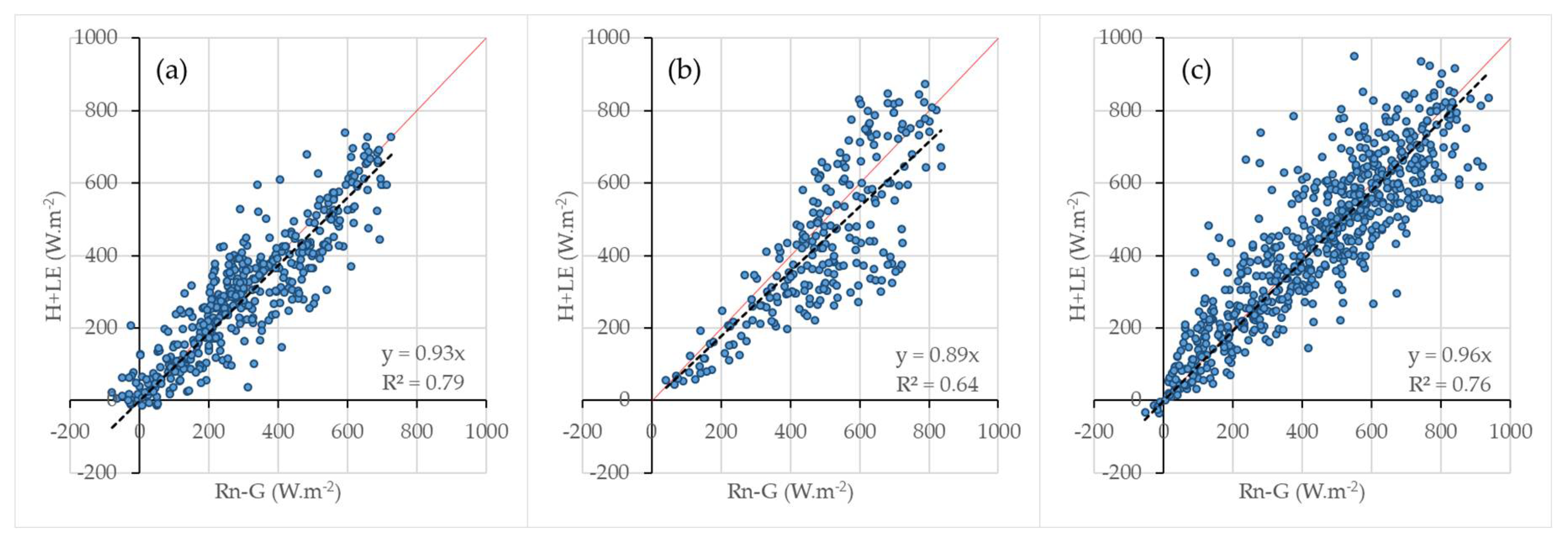
3.1. Energy Balance Closure for Flux Measurements

According to References [48,66,67], measures of H and LE tend to be underestimated by EC systems due to sources of errors such as non-homogeneous surface coverage, soil characteristics, instrumental errors, topography, divergence or flux dispersion, among others. In this sense, for METRIC processing dates (Table S1) the accuracy of EC data was checked using the energy balance closure for USR, PDG, and RECOR experimental sites for daytime flux measurements (8:00–18:00), as shown in Figure 2.
The hourly ratio of (H + LE) to (Rn − G) was unbalanced by 7%, 11%, and 4% for USR, PDG and RECOR sites, respectively, and the t-test indicated that the slope of the regression line through the origin was statistically different from unity, with a 95% confidence level. According to References [48,65] these are small uncertainties and can be corrected using the Bowen-ratio approach. In this manner, we applied this method to correct H and LE observed values, which were later used to validate METRIC estimations.

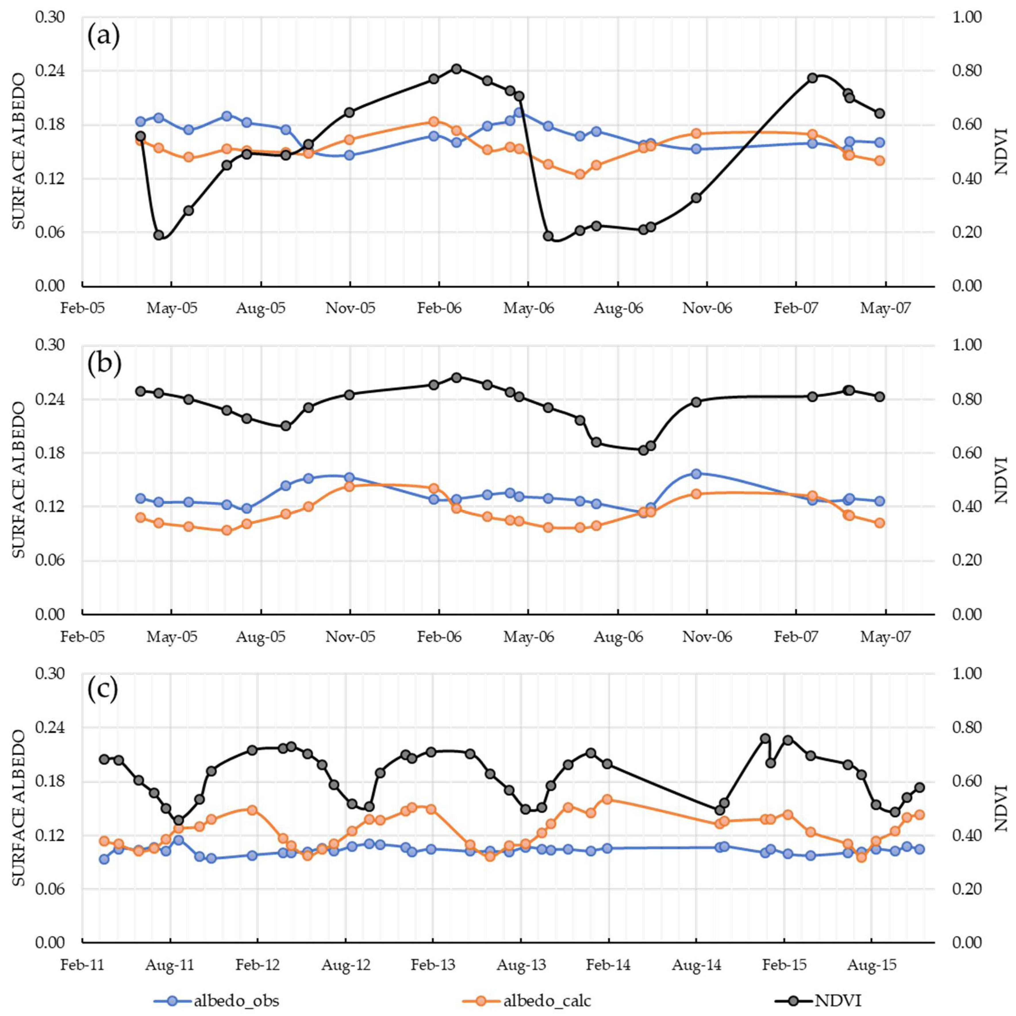
3.2. Broadband Surface Albedo

At the USR site, Equation (3) underestimated surface albedo by 10% (R2 = 0.94, MAE = 0.02 and RMSE = 0.03), with a 95% confidence level (Table 5), presented in Section 3.3. The temporal profile presented in Figure 3a shows that the observed values vary during the sugarcane cycle, with higher values at the initial stage, when there is a greater contribution of soil in surface reflectance [49]. During the crop development (indicated by an increase in NDVI—Figure 3a), observed surface albedo decreases from 0.18–0.20 (at initial stage) to values around 0.15, due to the thickening of sugarcane canopy, which favors the extinction/absorption of solar radiation. At the maturation stage (after the wet to dry season transition) albedo increases again (reaching values of 0.20) due to a reduction in leaf area index and to the presence of senescent leaves, which alters the crop reflectance patterns [68]. The reduction in observed and estimated albedo on 5 May 2005 is an effect of soil moisture reducing reflectance, caused by isolated precipitation in the experimental area in days prior to simulation [49]. For June 2005 and July 2006 cycles the estimated surface albedo for sugarcane ranged from 0.13 to 0.18, similar to that described by Reference [69] for sugarcane in Red-Yellow Latosol and mechanical harvesting with straw burning. The adjusted equation showed a better performance for vegetative growth stage (full crop coverage), but at initial and maturation stages we observed a tendency to underestimate surface albedo, possibly due to a greater contribution of soil in the reflectance. In addition, at the beginning of the two evaluated cycles, burning of harvest straw, soil plowing, and fertilization were carried out (procedures that decrease the reflectance observed by satellite). In the maturation stage, underestimates also occur, possibly due to residual soil moisture which decreases reflectance.
At the PDG site, surface albedo was underestimated by 15% (R2 = 0.94, MAE = 0.02, and RMSE = 0.02), with a 95% confidence level. The observed albedo presents a seasonal variation, with an average value (α = 0.13) smaller than that observed at the USR site (α = 0.17). The lowest values occur during the dry season (α ≅ 0.12), increasing gradually up to 0.16 in the dry to wet season transition. In the dry season, Ki penetrates more easily into the canopy, and thus the soil covered by dark plant litter absorbs more radiation, reducing the albedo [49]. In the rainy season, on the other hand, the albedo is controlled by tree canopy reflectance, which creates shade on the ground and dominates the absorption of photosynthetically active and near-infrared radiation. During the year the adjusted albedo equation tends to underestimate this variable, especially during the dry season, which could be an effect of the interaction of Ki with tree canopy and substrate, which presents a dynamic of alternation in albedo control between wet and dry seasons. A better performance is observed for the wet season, when there is a greater vegetative vigor (indicated by higher NDVI values) and the woody vegetation canopies dominate the reflectance.
For the sensu-strictu savanna at RECOR site, the adjusted model overestimated the surface albedo by 21%, with a 95% confidence level (R2 = 0.96, MAE = 0.02 and RMSE = 0.03). The observed albedo shows lower values (0.09 to 0.12) than those obtained for PDG woody savanna (0.12 to 0.16) and does not show the same seasonal variability. The estimated albedo values, on the other hand, follow the NDVI series for the study period, varying between 0.09 and 0.16, with an increase in the wet season caused by a higher reflectance due to a greater amount of green vegetation, both in woody and grassy areas.

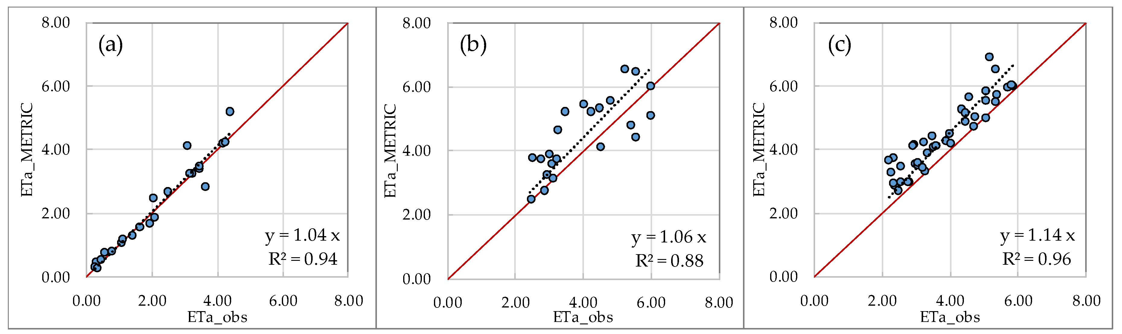
3.3. Validation of Energy Balance Fluxes

Table 5 presents a comparison between observed and estimated values of α, Rn, G, H, and LE, at the time of satellite overpass. For USR site (Figure 4a), the t-test indicated that Rn was overestimated by 9% (R2 = 0.93, MAE = 59.84 W m−2, RMSE = 75.36 W m−2), which is mainly due to underestimation of surface albedo at the crop initial stage. In vegetative growth and maturation stages the estimated Rn values were closer to 1:1 line, due to a better adjustment of the albedo submodel for conditions of full vegetation cover. It was found that the land surface temperature of MOD11 was underestimated by up to 10% at the dates when Rn was overestimated, which reduces the long wave radiation flux emitted by the surface and consequently increases Rn. Considering the study period, Rn ranged from 408 W m−2 to 728 W m−2, close to those presented by Reference [70] for the same crop. As observed by Reference [49], Rn presents a seasonal pattern, mainly controlled by Ki, surface albedo, and land surface temperature. Regarding the longwave component, Lw↓ ranged from 310 to 365 W m−2, following the seasonal variations of air temperature. Lw↑, in a similar way, varied according to the surface temperature, ranging from 403 to 489 W m−2 (see Figure S7 on the Supplementary Material). G estimates for USR site did not show good agreement with the observed values, being underestimated by 31% (R2 = 0.76), demonstrating that this submodel does not satisfactorily represent the reality for this landscape context. Sensible heat flux was overestimated by 26% (R2 = 0.86), showing low correlation with the observed values. According to Reference [70], values of H for sugarcane in the wet season are controlled by Rn, while in dry season the maturation or harvest of the crop favors the H contribution in the energy partitioning, due to a lower leaf area index. During the wet season, the relative errors for H varied between −1% and 18%, while Reference [70] obtained relative errors up to 70% using SEBAL/METRIC. For LE, the estimated/observed values present a balanced distribution around the 1:1 line (Figure 4a), with R2 = 0.94, MAE = 16.93 W m−2 and RMSE = 21.43 W m−2 (Table 5). The t-test indicated that the ratio of the estimated / observed values was significantly different from unity, suggesting that METRIC underestimated LE by 5%. This result shows that the errors in previous estimates were caused by the internal calibration in H estimates [46,71]. Instantaneous LE estimates ranged from 197 to 569 W m−2 during the two sugarcane growth cycles, near the values obtained by Reference [70] for the same sugarcane area, that ranged from 146 W m−2 to 529 W m−2.
At the PDG site (Figure 4b) Rn was overestimated by 9% (R2 = 0.84, MAE = 58.83 W m−2, RMSE = 67.95 W m−2), due to albedo underestimates and deviations in Ts, as verified for the USR site. METRIC estimates for this variable ranged from 454 to 772 W m−2, with values generally higher than those obtained for the USR site at each date. This is a result of the albedo lower values in the woody savanna (Figure 3), as well as lower values of Ts (which reduce the longwave radiation emitted by the surface). Lw↓ and Lw↑ ranged from 290 to 357 W m−2 and from 394 and 477 W m−2, respectively (Figure S7b), following the seasonal variation of air and surface temperatures. According to the t-test, G was overestimated by 39% (R2 = 0.54) and H was underestimated by 42% (R2 = 0.75). However, for LE the t-test indicated that b was significantly equal to unity, indicating that LE estimated by METRIC and in-situ measurements were similar (R2 = 0.92 MAE = 48 W m−2 and RMSE = 56 W m−2). METRIC estimated LE values from 107 to 520 W m−2 at this site, following the seasonal variation of available energy and NDVI (Figure 3b).
The ratio between estimated and observed values of Rn at RECOR site (Figure 4c) was significantly equal to unity, with a 95% confidence level (R2 = 0.96, MAE = 37 W m−2, RMSE = 47 W m−2), showing that METRIC is effective in estimating this variable with MODIS data. Instantaneous Rn estimates ranged from 504 to 779 W m−2, with an average 7% higher than that obtained at the PDG site. Lw↓ varied between 308 and 370 W m−2, while Lw↑ ranged from 387 to 465 W m−2 (Figure S7c), values close to those obtained for woody savanna at PDG site. For G estimations, the model showed poor performance by overestimating this flux by 210% (R2 = 0.67). Sensible heat flux was underestimated by 30% with R2 = 0.92) W m−2, absorbing previous deviations in its internal calibration. This led to accurate estimates of LE, whose values were considered equal to in-situ measurements by the t-test (b = 1), with a 95% confidence level.

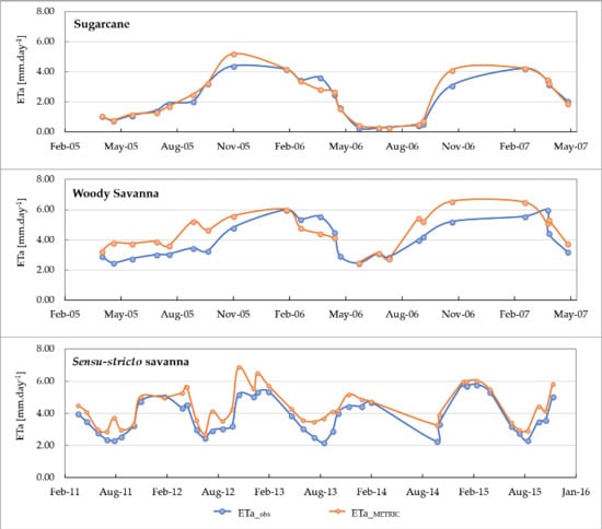
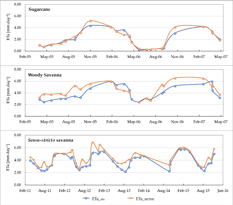
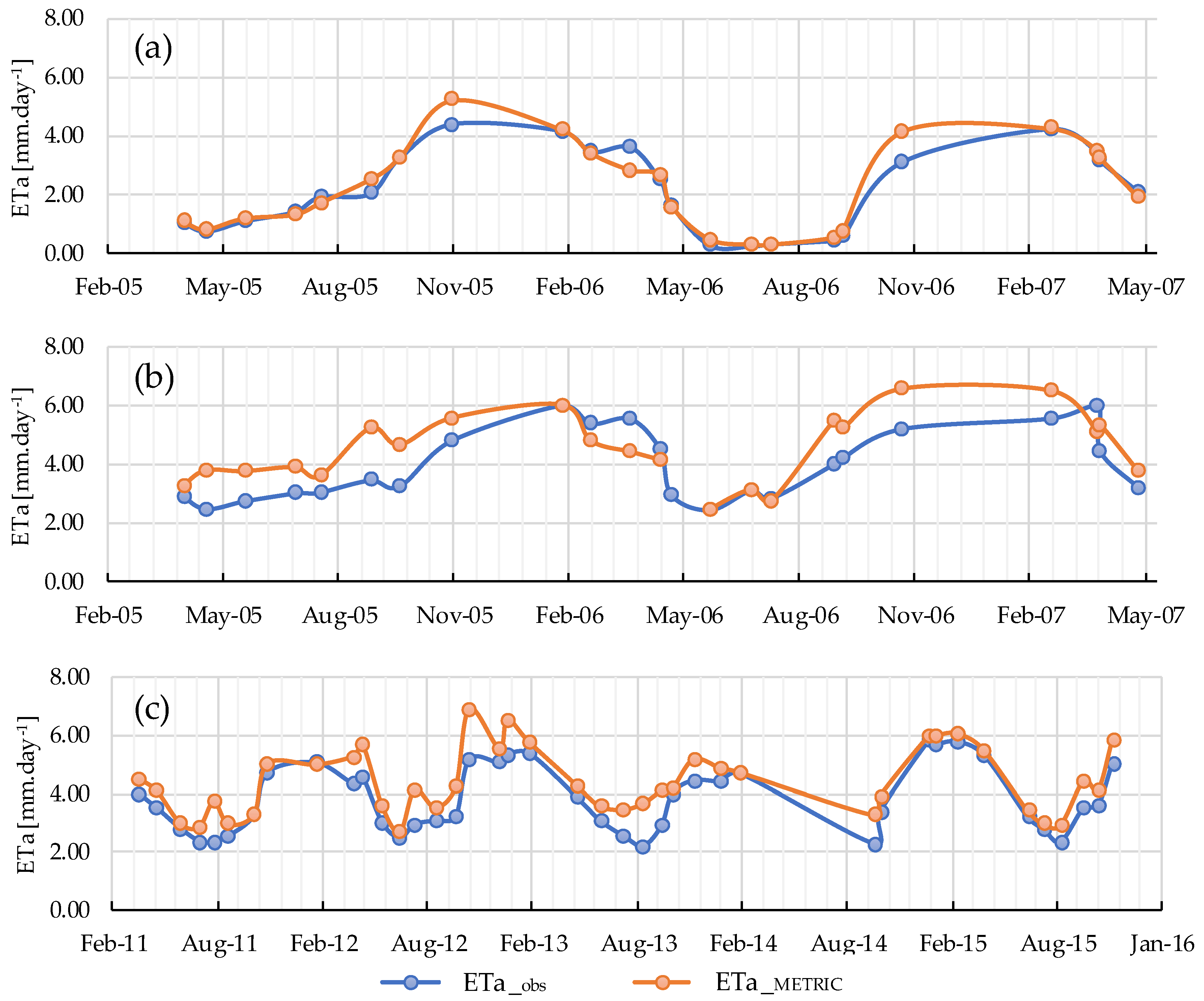
3.4. Reference Evapotranspiration Fraction (F) and Actual Evapotranspiration (ETa)

The METRIC model assumes that the reference evapotranspiration fraction (F) is constant throughout the day for well-watered agricultural crops [65], and can be considered equal to its crop coefficient (Kc). Thus, we tested this assumption using the statistical analysis presented in Table 6. The test consists of (i) comparing the instantaneous (at satellite overpass time) F obtained from the eddy covariance system (Fi_ec) with the mean values of daytime hourly F (Fmean) and; (ii) comparing Fi_ec with the Kc obtained from EC system (Kc_ec), as performed by Reference [46]. Table 6 shows that the assumption was considered valid for the three experimental sites, which indicates that F was approximately constant during the daytime under clear sky conditions (with a confidence level of 95%), for different phenological stages of both sugarcane and natural vegetation. Thus, we applied Equation (15) to extrapolate our ETa estimates from instantaneous to daily values.
Table 6 indicates that the crop coefficients estimated by METRIC for sugarcane (USR site) were significantly equivalent to those measured by the EC system (Kc_metric = Kc_ec), according to the t-test, with a 95% of confidence level. The temporal profile of sugarcane Kc in the June 2005 and July 2006 cycles is shown in Figure 5, and grouped according to the crop phenological phases, as described in References [22,72]. The deviations obtained in Kc_metric at some dates may have been caused by spectral mixing of different land cover types within the same MODIS pixel (1 km for Kc), with different reflectance values and surface temperature [73]. The mean estimated Kc values per phenological stage were 0.16 for germination, 0.57 for tillering, 0.57 for vegetative growth and 0.50 for maturation stages, while Reference [22] indicates values of 0.40, 1.25, and 0.75 for the initial, development and late stages, respectively. Reference [74] estimates the sugarcane Kc at the initial stage (up to 50 days after planting) between 0.35 and 0.40, which was obtained in this study for the June 2005 cycle. During this period, the rainfall was above average, which increased the water availability allowing a more accentuated growth than that for the July 2006 cycle.
ETa estimates for the USR site (Figure 6a) are close to the 1:1 line, with some estimate deviations during the rainy season. It is important to point out that for these dates it was difficult to select suitable hot pixels for the internal calibration, because the agricultural areas were almost entirely covered with the sugarcane crop. But in general METRIC performed well in estimating ETa (R2 = 0.94, MAE = 0.21 mm day−1 and RMSE = 0.35 mm day−1), as indicated by the t-test (b = 1, with a 95% confidence level). The temporal profile of ETa for sugarcane (Figure 7a) shows that during the two cycles ETa varied according to crop development (indicated by Kc in Figure 5 and NDVI in Figure 3a), the rainfall distribution, and energy availability (data not shown). Estimated ETa ranged from 0.29 mm day−1 to 5.21 mm day−1, with lower values occurring after harvest (when ETa is dominated by soil evaporation), gradually increasing to the highest values at peak development (higher water availability and leaf area index), followed by a decrease in the maturation stage (senescence of leaves reduces transpiration and increases H) [75].
In the woody savanna of PDG site, the t-test also indicated that the estimated F(Kc_metric) as well as the ETa estimates were equivalent to the measured values (b = 1), with a 95% confidence level. Figure 7b shows that the estimated ETa varied between 2.48 and 6.56 mm day−1 with the same seasonal pattern verified on the USR site, despite having higher values. For this area, Reference [52] observed ETa values varying from 1.0 mm day−1 (dry season of 2010) to 7.1 mm day−1 (summer season of 2012), and Reference [4] obtained an average value of 2.81 mm day−1 for the wet season and 1.70 mm day−1 for the dry season between 2001 and 2003.
For the sensu-stricto savanna of the RECOR site, unlike the other experimental sites, the t-test indicated that b values for Kc and ETa validation were significantly different from unity, then METRIC overestimated Kc by 11% (R2 = 0.96, MAE = 0.07 and RMSE = 0.08) and ETa by 14% (R2 = 0.96, MAE = 0.62 mm day−1 and RMSE = 0.75 mm day−1), with a 95% confidence level. Figure 6c shows that the ETa estimates were always above the 1:1 ratio line, which indicates that METRIC tended to overestimate daily ET during both wet and dry seasons over the sensu-stricto savanna. The ETa profile presented in Figure 7c shows that the estimated ETa varied between 2.71 and 6.91 mm day−1, following the same seasonal pattern obtained in PDG site: higher values during the wet season and lower values during the dry season.

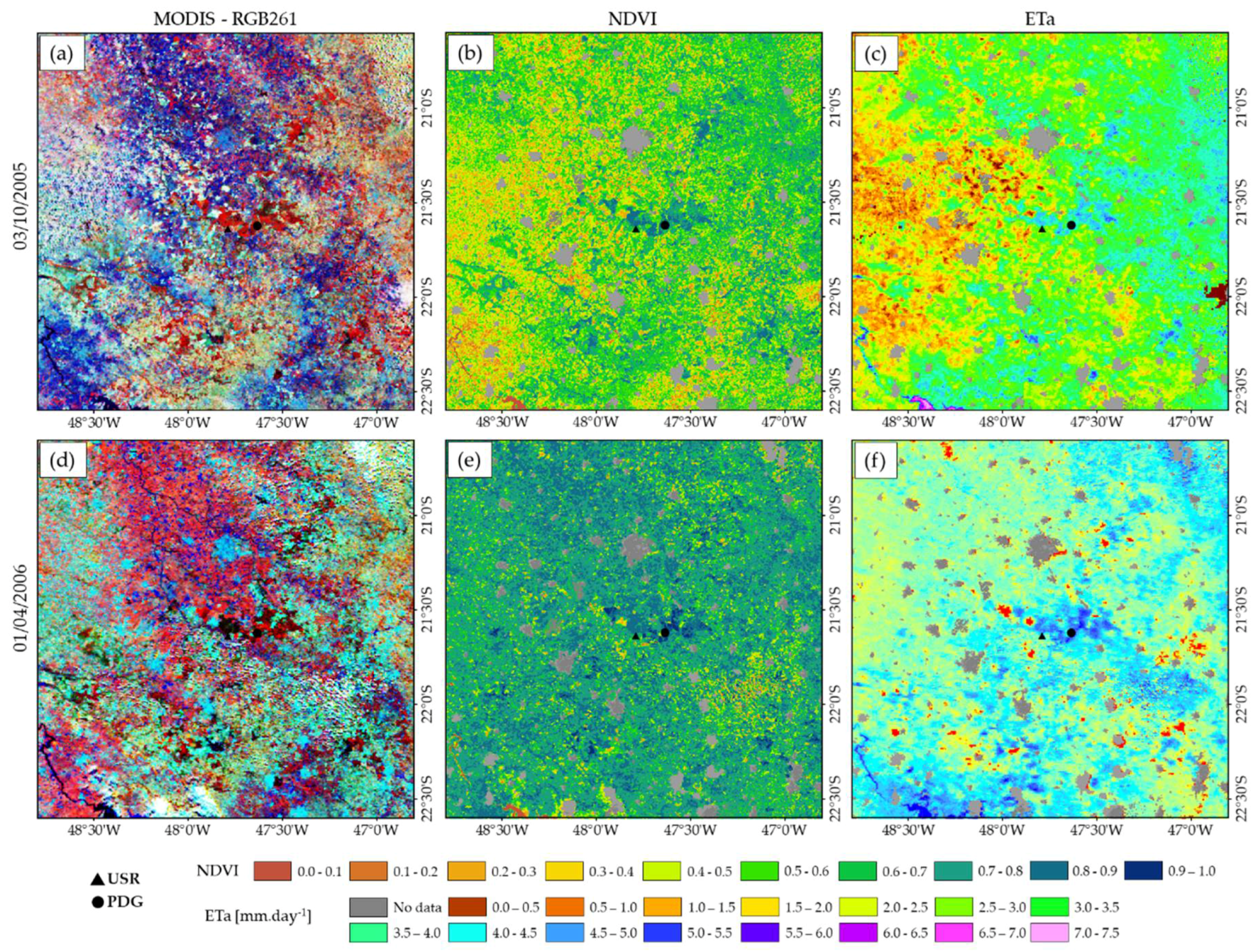
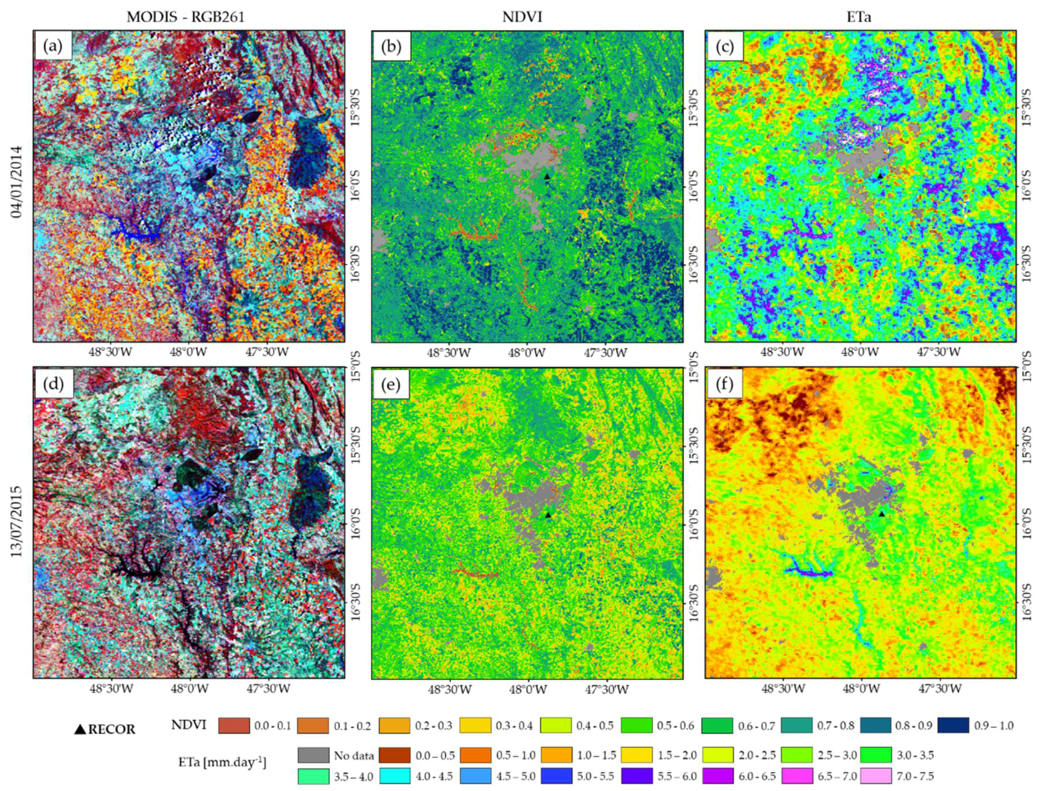
3.5. Spatial Distribution of ETa

Figure 8 and Figure 9 present the spatial distribution of ETa for São Paulo State and Federal District AOIs, illustrating the difference in the patterns observed during the dry and wet seasons. For the São Paulo AOI ETa varies between the dry and the wet seasons, reflecting the conditions of soil water availability, precipitation distribution (Figure S2a,b), and vegetative vigor (the increase of ETa when the sugarcane crop is at full development during the wet season). The 3 October 2005 image is from the dry to wet season transition, when the sugarcane crop is still in the harvest period, with several areas of bare soil (dark blue) or covered with straw left on the soil after harvesting (cyan), which are the same areas that appear in bright red (fully vegetated) in the 1 April 2006 image (Figure 8d). In the dry season, NDVI and ETa values (Figure 8b,c, respectively) are generally lower for agricultural areas than those in the wet season (Figure 8e,f, respectively). On 1 April 2006, sugarcane is at maximum vegetative vigor (bright red in Figure 8d), presenting higher NDVI (mean of 0.78) and maximum values of ETa reaching 4.5 mm day−1. The area around PDG site shows the highest values of NDVI and ETa both in dry and wet seasons, since it is a region surrounded by reforestation and Cerrado woodlands.
At the Federal District AOI, the agricultural areas (see Figure S1) on 4 January 2014 (Figure 9a) are at full vegetative vigor (soybean crop in yellow and maize in red, mainly), with NDVI and ETa values above 0.9 and above 6.0 mm day−1, respectively. In these areas there are rain fed and irrigated fields, causing variability in ETa values estimated by METRIC. In an irrigated field, soil water availability is higher, which associated to a high evaporative demand (characteristic of this region) leads to higher ETa values. On 13 July 2015 (Figure 9b) NDVI values are generally smaller throughout this AOI (even for natural vegetation areas), but high values of NDVI (0.9) and ETa (above 4 mm day−1) occur in areas of irrigated agriculture (predominantly maize crop). However, for a large part of the AOI, low ETa values occur (<1.0 mm day−1), evidence of a reduction in soil moisture during the dry season.

4. Discussion

The albedo submodel was adapted for the study areas and applied with MOD09 data as input, but the t-test indicated, with a 95% confidence level, that albedo was underestimated at the USR and PDG sites by 10% and 15%, respectively, and overestimated by 21% at RECOR site (Table 5). For the USR site, Equation (3) presented a better result when compared to those obtained by Reference [76] for this experimental site with the equations proposed by Reference [36,55], which underestimated the surface albedo by 19% and 24%, respectively. We must also consider that during the harvest season there may be spectral mixing of harvested areas and sugarcane crop within the MODIS pixel (Figure S5 on the Supplementary Material). Moreover, for taller vegetation (as woody savanna), deviations in estimated albedo may occur in situations where the sun is not at its zenith, which causes the mixing of sunlit and shaded areas in the same pixel, particularly in the winter months, when the solar zenith angle is higher [59].
The method applied to estimate surface albedo does not correct for any bidirectional reflectance distribution function (BRDF) caused by off-nadir sensor view angles, such as those occurring in MODIS images (sensor view angles up to 55 degrees), where backscattering or forward scattering directions causes deviations in the reflected signals to sensor [36]. Then, for dates where the sensor view angle was close to 20 degrees off-nadir (maximum sensor view angle recommended by [77]), the accuracy of MOD09 surface reflectance may be affected due to lack of consideration of BRDF, leading to deviations in the estimated surface albedo. In addition, MOD09 atmospheric correction does not take into consideration local atmospheric parameters, which can lead to errors [78].
NDVI values for PDG site (woody savanna) ranged from 0.60 to 0.80, while for RECOR (sensu-stricto savanna) it varied between 0.50 and 0.75, but both presented the same seasonal pattern, following the rainfall distribution (Figure S2) [39]. At the time when NDVI reaches its maximum value, the estimated albedo begins to decrease, due to the shade provided by taller tree canopies, which favors the extinction of solar radiation at the surface and reduces the reflected shortwave radiation. NDVI decreases during the dry season can be attributed to leaf abscission that occurs during the wet to dry season transition for many Cerrado tree species [79]. The observed values of albedo in the RECOR site do not present the same seasonal variation observed for the woody savanna of the PDG site, possibly due to the spatial distribution of the different vegetal species in stricto-sensu savanna, where the woody and grassy vegetation mixture does not present the same alternation in albedo control observed for woody savanna.
Net radiation was satisfactorily estimated by METRIC at the stricto-sensu savanna but overestimated by 8% and 9% at sugarcane and woody savanna experimental sites, respectively, possibly due to deviations in the estimated surface albedo or to the land surface temperature obtained from MOD11. Our results showed a better fit than those obtained by Reference [1] (R2 = 0.83 for sugarcane and R2 = 0.88 for savanna), but with higher RMSE ([1] obtained RMSE = 37 W m−2 for sugarcane and RMSE 47 W m−2 for savanna). Rn is typically higher during the wet season, which is a typical pattern for the Cerrado biome [1,79], although it is the opposite of that observed for the humid evergreen forest of the Amazon Basin, where prolonged cloud cover tends to reduce wet-season Rn [80]. For Cerrado vegetation, the decline in Rn during the dry season is due not only to lower solar radiation, but also in part to an increase in the surface albedo (Figure 3) caused by a reduction in vegetation leaf area and/or greenness during the dry season, when soil water availability is low [79]. The longwave components of Rn (Lw↓ and Lw↑) are estimated using the Stefan-Boltzmann law (Equations (10) and (12)), therefore, they are directly influenced by air and surface temperatures, respectively [60]. Thus, for the three experimental sites, Lw↓ and Lw↑ curves have a slight increase during summer, when both air and surface temperatures are higher. Comparing these two components (Figure S7), Lw↑ presented higher values than Lw↓, once surface temperature obtained from MOD11 was higher than air temperature (at satellite overpass time). Hence, the resulting longwave component of Rn is always negative, with a seasonal variation less pronounced than that observed for the shortwave component. Considering the three experimental sites evaluated, Rn ranged from 272.34 W m−2 (sugarcane) to 837.80 W m−2 (sensu-stricto savanna). As these estimates are obtained at satellite overpass time (~10:30), and since measurements by remote sensing are possible for clear sky days, our results for METRIC processing days represent the instances of greater energy availability to the biophysical processes [70].
Regarding G, METRIC estimates showed low agreement with field measurements for all experimental sites. Generally, this flux is the one that presents the biggest modeling errors with satellite data, since it is an empirical approximation specifically calibrated for semi-arid areas and may not accurately represent the local conditions of our study area [1,18,33,70,81], and these errors can be associated with the difference of spatial and temporal scales between satellite data and in situ measurements [23,65].
LE estimates were significantly equal to observations for PDG and RECOR sites, but underestimated for the sugarcane experimental site, although only by 5%. The estimated values of LE ranged from 18.8 W m−2 to 376.53 W m−2 in the sugarcane field (USR site), 107 to 520 in PDG site and 197 to 569 W m−2 in RECOR site (sensu-stricto savanna), following the seasonal pattern indicated by Reference [1] for sugarcane and by Reference [79] for a mixed grassland savanna in Mato Grosso, Brazil. The accuracy in LE estimations depends on the anchor pixel selection, which determines the self-calibration of H [65]. Thus, the biases in H are necessary because its intern calibration absorbs errors derived from other steps in previous estimates (such as albedo, Rn, and G) [65,71,82].
Our results corroborate to the assumption that F is constant throughout the day (and is equivalent to Kc) at the three experimental sites, showing that the METRIC method for extrapolating from instantaneous to daily ET is valid for heterogeneous surfaces containing agricultural and natural Cerrado vegetation. According to Reference [23] Kc values for heterogeneous surfaces depend on canopy geometry, plant density, and on adopted agricultural practices, which determine the ET partition between transpiration and evaporation. For sugarcane it was verified that Kc varied in each phenological stage according to increases in leaf area index and water availability. Kc values below those referenced by Reference [22], especially for vegetative growth stage, may be due to the spatial resolution for Kc maps (1 km), which can mix different land cover types with sugarcane in the same pixel.
Overall, METRIC was effective at estimating ETa at USR and PDG sites, with a 95% confidence level. For the RECOR site, ETa was overestimated by 14%, with R2 and RMSE close to those reported in the literature. Reference [83] reported values of R2 ranging from 0.45 to 0.95 and RMSE varying between 10 to 30% for ETa estimates in natural ecosystems using remote sensing based models, and stated that the uncertainty associated with remote sensing estimates of ET is constrained by the accuracy of ground measurements, for which for the flux tower data are in the order of 10–30%. For fully covered crops, several studies [11,17,65,84] have indicated that METRIC could present absolute errors between 5–20% in the daily ETa estimate. Reference [59] obtained R2 = 0.67 and RMSE = 0.81 mm for a Tropical semideciduous forest, in which METRIC tended to overestimate daily ET in comparison to EC flux tower data. They report that the error can be associated with the selection of cold pixels, since in their study area there are no ideal agricultural areas to be selected for cold pixels.
Sugarcane ETa presented a higher variability (ranging from 0.29 to 5.21 mm day−1) due to crop variation from bare soil in the beginning of the cycle, when ET is controlled mainly by soil evaporation, to the maximum vegetative vigor, when the NDVI and leaf area index reach their maximum values. However, the woody savanna ETa was always higher, even in the dry season, because of the greater density of the woody component (predominantly deep rooted), that can draw water stored in deeper soil compartments. According to Reference [39] deep soil compartment can contribute to as much as 83% of the total water used in a tree-dominated Cerrado landscape, also providing water for vegetation in other periods of high demand, such as in the transition from dry to rainy season. Reference [52] showed that, at the PDG site between 2009 and 2012, despite a 11% increase in the annual rainfall observed in an analysis year, water use increased by 4%, while a 16% decrease in rainfall (in the subsequent year) did not affect ET. They also observed that in woody savanna the vegetation exhibited a strong surface control in parallel with a decrease in leaf area index, thus reducing the demand for water on a gradually declining water availability, an evidence of its adaptation to this seasonally dry climate.
Seasonality in ETa estimates at the RECOR site was comparable to those obtained for the PDG site, with minimum values occurring at the end of the dry season, indicating that the reduced water availability constrained dry season ETa at both sites. Differences in maximum and minimum values may be a result of the savanna vegetation spatial heterogeneity, enhanced by the distinctive leaf phenology of the species [52,85,86]. Comparing two phytophysiognomies (cerrado denso and campo sujo) during the dry and wet seasons, Reference [39] estimated ETa ranging from 1.4 to 5.8 mm day−1 for cerrado denso and from 0.9 to 4.5 mm day−1 for campo sujo. They stated that the differences in the two ecosystems are associated not only with differences in root distribution, but also with differences in tree densities and phenology of full-leaf canopies. In general, METRIC showed a good performance, considering that Reference [17] had suggested that remote sensing-based ETa estimates with similar biases are considered as acceptable.

5. Conclusions

We evaluated METRIC model performance to estimate the energy balance and ET in heterogeneous areas in the Brazilian cerrado. Flux tower data from sugarcane, woody savanna, and sensu-stricto savanna were used to validate METRIC estimates. The surface albedo model was adapted applying the SMARTS2 model, leading to deviations between 10–21% and maximum RMSE = 0.03.
Our results suggest that METRIC is effective for simulating the energy balance and ET spatial and temporal variability over agricultural and natural land covers in the Brazilian Cerrado with relative accuracy. Overall, METRIC performed well for Rn (R2 > 0.94) and LE (R2 > 0.93), leading to accurate ETa estimates for USR and PDG sites (R2 = 0.94 and R2 = 0.88, respectively) but showed an overestimation of 14% for the RECOR site.
Furthermore, the assumption that F is constant throughout the day and can be used to extrapolate instantaneous to daily ET values was tested and validated for our three experimental sites. For sugarcane we obtained Kc curves covering its phenological stages, which can be applied in yield models for this crop in future studies.
Sugarcane energy balance fluxes and ET varied throughout the crop cycles, showing dependence on available energy, rainfall, albedo, and NDVI. For the natural cerrado vegetation, ET was mainly controlled by the seasonal variation of net radiation, rainfall, and surface water availability. Our results reproduced a typical pattern for the Brazilian cerrado, which is marked by the seasonality of leaf area index and green biomass.
Many species of woody and stricto-sensu savannas have deep root systems, which allow transpiration to be maintained even during the dry season. Thus, the conversion of undisturbed cerrado to grass-dominated or agricultural crops (combined with a higher fire frequency) has the potential to change the energy balance by increasing surface albedo and temperature [10], as well as water balance, by increasing runoff and groundwater recharge, decreasing canopy interception and reducing ET due to less water uptake by deep roots (especially during the dry season).Therefore, assuming the local precipitation is reliant on regional rates of ET, the cerrado climate could become drier [4,39,52,87]. Lastly, as the Brazilian Cerrado is a large biome with different conditions of land cover, soil types, vegetation, and hydrometeorology, it is necessary to carry out more studies in different regions in order to improve our understanding of ET dynamics.

Supplementary Materials

The Supplementary Materials are available online at https://www.mdpi.com/2072-4292/10/8/1181/s1.

Author Contributions

B.S.O., E.C.M. and M.C.-B. design the research. B.S.O., M.C.-B., G.B. and G.A.V.M. processed the data. B.S.O., E.C.M. and M.C.-B. contributed to the analysis and interpretation of the results. B.S.O. and E.C.M. wrote the paper and all the other members revised it.

Acknowledgments

We acknowledge the people involved in LBA project and IAG-USP who worked in the field data collection. Bruno Silva Oliveira acknowledges the Brazilian Ministry of Science and Technology and Brazilian Ministry of Education for providing research fellowships through the CNPq (Grant No. 140068/2016-3) and CAPES (Grant No. 33010013005PO) agencies.

Conflicts of Interest

The authors declare no conflict of interest.

References

  1. Ruhoff, A.L.; Paz, A.R.; Collischonn, W.; Aragao, L.E.O.C.; Rocha, H.R.; Malhi, Y.S. A modis-based energy balance to estimate evapotranspiration for clear-sky days in Brazilian Tropical Savannas. Remote Sens. 2012, 4, 703–725. [Google Scholar] [CrossRef]
  2. Sano, E.E.; Rosa, R.; Brito, J.L.S.; Ferreira, L.G. Mapeamento de Cobertura Vegetal do Bioma Cerrado: Estratégias e Resultados; Embrapa Cerrados: Planaltina, DF, Brazil, 2007; p. 30. ISSN 1517-5111. [Google Scholar]
  3. MMA, M.d.M.A.O. Ppcerrado—Plano de Ação Para Prevenção e Controle do Desmatamento e das Queimadas no Cerrado:2ª Fase (2014–2015); Instituto do Meio Ambiente e dos Recursos Naturais Renováveis: Brasília, DF, Brazil, 2014; p. 132. [Google Scholar]
  4. Oliveira, P.T.S.; Wendland, E.; Nearing, M.A.; Scott, R.L.; Rosolem, R.; da Rocha, H.R. The water balance components of undisturbed tropical woodlands in the brazilian cerrado. Hydrol. Earth Syst. Sci. 2015, 19, 2899–2910. [Google Scholar] [CrossRef]
  5. WWF. The Growth of Soy: Impacts and Solutions; World Wildlife Fund International: Gland, Switzerland, 2014; p. 96. [Google Scholar]
  6. Instituto Brasileiro do Meio Ambiente e dos Recursos Renováveis (IBAMA); Ministério do Meio Ambiente (MMA); United Nations Development Programme (UNDP). Monitoramento do Desmatamento nos Biomas Brasileiros por Satélite. Available online: http://siscom.ibama.gov.br/monitora_biomas/ (accessed on 21 January 2017).
  7. Grecchi, R.C.; Gwyn, Q.H.J.; Bénié, G.B.; Formaggio, A.R.; Fahl, F.C. Land use and land cover changes in the brazilian cerrado: A multidisciplinary approach to assess the impacts of agricultural expansion. Appl. Geogr. 2014, 55, 300–312. [Google Scholar] [CrossRef]
  8. Da Silva, B.B.; Wilcox, B.P.; da Silva, V.d.P.R.; Montenegro, S.M.G.L.; de Oliveira, L.M.M. Changes to the energy budget and evapotranspiration following conversion of tropical savannas to agricultural lands in São Paulo state, Brazil. Ecohydrology 2014, 8, 1272–1283. [Google Scholar] [CrossRef]
  9. Ramankutty, N.; Foley, J.A.; Olejniczak, N.J. People on the land: Changes in global population and croplands during the 20thcentury. AMBIO J. Hum. Environ. 2002, 31, 251–257. [Google Scholar] [CrossRef]
  10. Loarie, S.R.; Lobell, D.B.; Asner, G.P.; Mu, Q.; Field, C.B. Direct impacts on local climate of sugar-cane expansion in Brazil. Nat. Climat. Chang. 2011, 1, 105–109. [Google Scholar] [CrossRef]
  11. Gowda, P.H.; Chavez, J.L.; Colaizzi, P.D.; Evett, S.R.; Howell, T.A.; Tolk, J.A. Et mapping for agricultural water management: Present status and challenges. Irrig. Sci. 2007, 26, 223–237. [Google Scholar] [CrossRef]
  12. Agência Nacional de Águas. Conjuntura dos Recursos Hídricos: Informe 2016; Agência Nacional de Águas: Brasilia, DF, Brasil, 2016; p. 96.
  13. Jung, M.; Reichstein, M.; Ciais, P.; Seneviratne, S.I.; Sheffield, J.; Goulden, M.L.; Bonan, G.; Cescatti, A.; Chen, J.; de Jeu, R.; et al. Recent decline in the global land evapotranspiration trend due to limited moisture supply. Nature 2010, 467, 951–954. [Google Scholar] [CrossRef] [PubMed] [Green Version]
  14. Trenberth, K.E.; Fasullo, J.T.; Kiehl, J. Earth's global energy budget. Bull. Am. Meteorol. Soc. 2009, 90, 311–323. [Google Scholar] [CrossRef]
  15. Mu, Q.; Zhao, M.; Running, S.W. Improvements to a modis global terrestrial evapotranspiration algorithm. Remote Sens. Environ. 2011, 115, 1781–1800. [Google Scholar] [CrossRef]
  16. Sellers, P.J.; Randall, D.A.; Collatz, G.J.; Berry, J.A.; Field, C.B.; Dazlich, D.A.; Zhang, C.; Collelo, G.D.; Bounoua, L. A revised land surface parameterization (sib2) for atmospheric gcms. Part I: Model formulation. J. Clim. 1996, 9, 30. [Google Scholar] [CrossRef]
  17. Kalma, J.D.; McVicar, T.R.; McCabe, M.F. Estimating land surface evaporation: A review of methods using remotely sensed surface temperature data. Surv. Geophys. 2008, 29, 421–469. [Google Scholar] [CrossRef]
  18. Ruhoff, A.L. Sensoriamento Remoto Aplicado à Estimativa da Evapotranspiração em Biomas Tropicais; Universidade Federal do Rio Grande do Sul: Porto Alegre, RS, Brazil, 2011. [Google Scholar]
  19. Meireles, M. Estimativa da Evapotranspiração Real pelo Emprego do Algoritmo Sebal e Imagem Landsat 5-tm na Bacia do Acaraú-Ce. Master’s Thesis, Universidade Federal do Ceará, Fortaleza, Brazil, 2007. [Google Scholar]
  20. Morton, C.G.; Huntington, J.L.; Pohll, G.M.; Allen, R.G.; McGwire, K.C.; Bassett, S.D. Assessing calibration uncertainty and automation for estimating evapotranspiration from agricultural areas using metric. J. Am. Water Resour. Assoc. 2013, 49, 549–562. [Google Scholar] [CrossRef]
  21. Anderson, M.C.; Allen, R.G.; Morse, A.; Kustas, W.P. Use of landsat thermal imagery in monitoring evapotranspiration and managing water resources. Remote Sens. Environ. 2012, 122, 50–65. [Google Scholar] [CrossRef]
  22. Allen, R.G.; Allen, R.G.; Food and Agriculture Organization of the United Nation. Crop Evapotranspiration: Guidelines for Computing Crop Water Requirements; Food and Agriculture Organization of the United Nations: Roma, Italy, 1998. [Google Scholar]
  23. De la Fuente-Sáiz, D.; Ortega-Farías, S.; Fonseca, D.; Ortega-Salazar, S.; Kilic, A.; Allen, R. Calibration of metric model to estimate energy balance over a drip-irrigated apple orchard. Remote Sens. 2017, 9, 670. [Google Scholar] [CrossRef]
  24. Folhes, M.T. Modelagem da Evapotranspiração para a gestão Hídrica de Perímetros Irrigados com Base em Sensores Remotos; Instituto Nacional de Pesquisas Espaciais: São José dos Campos, Brazil, 2007. [Google Scholar]
  25. ASCE-EWRI. The ASCE Standardized Reference Evapotranspiration Equation; Environmental and Water Resources Institute of the American Society of Civil Engineers: Kimberly, ID, USA, 2005; p. 70. [Google Scholar]
  26. He, R.; Jin, Y.; Kandelous, M.; Zaccaria, D.; Sanden, B.; Snyder, R.; Jiang, J.; Hopmans, J. Evapotranspiration estimate over an almond orchard using landsat satellite observations. Remote Sens. 2017, 9, 436. [Google Scholar] [CrossRef]
  27. Diak, G.R.; Mecikalski, J.R.; Anderson, M.C.; Norman, J.M.; Kustas, W.P.; Torn, R.D.; DeWolf, R.L. Estimating land surface energy budgets from space: Review and current efforts at the university of wisconsin—Madison and USDA–ARS. Bull. Am. Meteorol. Soc. 2004, 85, 65–78. [Google Scholar] [CrossRef]
  28. French, A.N.; Jacob, F.; Anderson, M.C.; Kustas, W.P.; Timmermans, W.; Gieske, A.; Su, Z.; Su, H.; McCabe, M.F.; Li, F.; et al. Surface energy fluxes with the advanced spaceborne thermal emission and reflection radiometer (aster) at the iowa 2002 smacex site (USA). Remote Sens. Environ. 2005, 99, 55–65. [Google Scholar] [CrossRef]
  29. Glenn, E.P.; Huete, A.R.; Nagler, P.L.; Hirschboeck, K.K.; Brown, P. Integrating remote sensing and ground methods to estimate evapotranspiration. Crit. Rev. Plant Sci. 2007, 26, 139–168. [Google Scholar] [CrossRef]
  30. Paiva, C.M.; Tsukahara, R.Y.; França, G.B.; Nicacio, R.M. Estimativa da evapotranspiração via sensoriamento remoto para fins de Manejo de Irrigação. In Proceedings of the XV Simpósio Brasileiro de Sensoriamento Remoto, Curutiba, PR, Brasil, 30 April–5 May 2011; p. 7. [Google Scholar]
  31. Liou, Y.-A.; Kar, S. Evapotranspiration estimation with remote sensing and various surface energy balance algorithms—A review. Energies 2014, 7, 2821–2849. [Google Scholar] [CrossRef]
  32. Allen, R.G.; Tasumi, M.; Trezza, R. Satellite-based energy balance for mapping evapotranspiration with internalized calibration (metric)—Model. J. Irrig. Drain. Eng. 2007, 133, 380–394. [Google Scholar] [CrossRef]
  33. Bastiaanssen, W.G.M. Sebal-based sensible and latent heat fluxes in the irrigated gediz basin, Turkey. J. Hydrol. 2000, 229, 87–100. [Google Scholar] [CrossRef]
  34. Gueymard, C. Smarts2: A Simple Model of the Atmospheric Radiative Transfer of Sunshine: Algorithms and Performance Assessment; Florida Solar Energy Center: Cocoa, FL, USA, 1995; Volume 1, p. 85. [Google Scholar]
  35. Ke, Y.; Im, J.; Park, S.; Gong, H. Downscaling of modis one kilometer evapotranspiration using landsat-8 data and machine learning approaches. Remote Sens. 2016, 8, 215. [Google Scholar] [CrossRef]
  36. Tasumi, M.; Allen, R.G.; Trezza, R. At-surface reflectance and albedo from satellite for operational calculation of land surface energy balance. J. Hydrol. Eng. 2008, 13, 51–63. [Google Scholar] [CrossRef]
  37. Silva, J.M.C.D.; Bates, J.M. Biogeographic patterns and conservation in the south american cerrado: A tropical savanna hotspotthe cerrado, which includes both forest and savanna habitats, is the second largest south american biome, and among the most threatened on the continent. BioScience 2002, 52, 225–234. [Google Scholar]
  38. Schwieder, M.; Leitão, P.J.; da Cunha Bustamante, M.M.; Ferreira, L.G.; Rabe, A.; Hostert, P. Mapping brazilian savanna vegetation gradients with landsat time series. Int. J. Appl. Earth Observ. Geoinf. 2016, 52, 361–370. [Google Scholar] [CrossRef]
  39. Oliveira, R.S.; Bezerra, L.; Davidson, E.A.; Pinto, F.; Klink, C.A.; Nepstad, D.C.; Moreira, A. Deep root function in soil water dynamics in Cerrado Savannas of Central Brazil. Funct. Ecol. 2005, 19, 574–581. [Google Scholar] [CrossRef]
  40. Simões de Castro, S.; Abdala, K.; Aparecida Silva, A.; Borges, V.M.S. A expansão da cana-de-açúcar no cerrado e no estado de goiás: Elementos para uma análise espacial do processo. Boletim Goiano de Geografia 2010, 30. [Google Scholar] [CrossRef]
  41. Rudorff, B.F.T.; de Aguiar, D.A.; da Silva, W.F.; Sugawara, L.M.; Adami, M.; Moreira, M.A. Studies on the rapid expansion of sugarcane for ethanol production in São Paulo state (Brazil) using landsat data. Remote Sens. 2010, 2, 1057–1076. [Google Scholar] [CrossRef]
  42. Peel, M.C.; Finlayson, B.L.; McMahon, T.A. Updated world map of the köppen-geiger climate classification. Hydrol. Earth Syst. Sci. 2007, 11, 1633–1644. [Google Scholar] [CrossRef]
  43. Cabral, O.M.R.; Rocha, H.R.; Gash, J.H.; Ligo, M.A.V.; Tatsch, J.D.; Freitas, H.C.; Brasilio, E. Water use in a sugarcane plantation. GCB Bioenergy 2012, 4, 555–565. [Google Scholar] [CrossRef] [Green Version]
  44. Steinke, V.; Palhares de Melo, L.; Torres Steinke, E. Rainfall variability in january in the federal district of brazil from 1981 to 2010. Climate 2017, 5, 68. [Google Scholar] [CrossRef]
  45. INMET, I.N.d.M. Normais Climatológicas do Brasil 1981–2010. Available online: http://www.inmet.gov.br/portal/index.php?r=clima/normaisclimatologicas (accessed on 27 April 2018).
  46. Carrasco-Benavides, M.; Ortega-Farías, S.; Lagos, L.O.; Kleissl, J.; Morales, L.; Poblete-Echeverría, C.; Allen, R.G. Crop coefficients and actual evapotranspiration of a drip-irrigated merlot vineyard using multispectral satellite images. Irrig. Sci. 2012, 30, 485–497. [Google Scholar] [CrossRef]
  47. Ortega-Farias, S.; Poblete-Echeverría, C.; Brisson, N. Parameterization of a two-layer model for estimating vineyard evapotranspiration using meteorological measurements. Agric. For. Meteorol. 2010, 150, 276–286. [Google Scholar] [CrossRef]
  48. Twine, T.E.; Kustas, W.P.; Norman, J.M.; Cook, D.R.; Houser, P.R.; Meyers, T.P.; Prueger, J.H.; Starks, P.J.; Wesely, M.L. Correcting eddy-covariance flux underestimates over a grassland. Agric. For. Meteorol. 2000, 103, 279–300. [Google Scholar] [CrossRef] [Green Version]
  49. Tatsch, J.D. Uma Análise dos Fluxos de Superfície e do Microclima Sobre Cerra, Cana-de-Açúcar e Eucalipto, com Implicações para Mudanças Climáticas Regionais. Master’s Thesis, Universidade de São Paulo, São Paulo, Brazil, 2006. [Google Scholar]
  50. Rocha, H.R.; Freitas, H.C.; Rosolem, R.; Juarez, R.I.N.; Tannus, R.N.; Ligo, M.A.; Cabral, O.M.R.; Dias, M.A.F.S. Measurements of co2 exchange over a woodland savanna (cerrado sensu stricto) in Southeast Brasil. Biota Neotropica 2002, 2, 11. [Google Scholar] [CrossRef]
  51. Furley, P.A. The nature and diversity of neotropical savanna vegetation with particular reference to the Brazilian Cerrados. Glob. Ecol. Biogeogr. 1999, 8, 223–241. [Google Scholar] [CrossRef]
  52. Cabral, O.M.R.; da Rocha, H.R.; Gash, J.H.; Freitas, H.C.; Ligo, M.A.V. Water and energy fluxes from a woodland savanna (cerrado) in Southeast Brazil. J. Hydrol. Reg. Stud. 2015, 4, 22–40. [Google Scholar] [CrossRef] [Green Version]
  53. Large-Scale Biosphere-Atmosphere Experiment in Amazonia, L. Lba Project—Federal District Tower. Available online: http://lba2.inpa.gov.br/index.php/torres/distrito-federal.html (accessed on 28 May 2016).
  54. Brazilian Institute of Geography and Statistics. Reserva Ecológica do Ibge: Ambiente e Plantas Vasculares; Brazilian Institute of Geography and Statistics: Rio de Janeiro, Brazil, 2004; p. 73.
  55. Liang, S. Narrowband to broadband conversions of land surface albedo I. Remote Sens. Environ. 2000, 76, 213–238. [Google Scholar] [CrossRef]
  56. Vermote, E.F.; Vermeulen, A. Atmospheric Correction Algorithm: Spectral Reflectances (mod09); Department of Geography, University of Maryland: College Park, MD, USA, 1999; p. 107. [Google Scholar]
  57. Wan, Z. Modis Land-Surface Temperature Algorithm Theoretical Basis Document; University of California: Santa Barbara, CA, USA, 1999; p. 77. [Google Scholar]
  58. Gao, Z.Q.; Liu, C.S.; Gao, W.; Chang, N.B. A coupled remote sensing and the surface energy balance with topography algorithm (sebta) to estimate actual evapotranspiration over heterogeneous terrain. Hydrol. Earth Syst. Sci. 2011, 15, 119–139. [Google Scholar] [CrossRef] [Green Version]
  59. Numata, I.; Khand, K.; Kjaersgaard, J.; Cochrane, M.; Silva, S. Evaluation of landsat-based metric modeling to provide high-spatial resolution evapotranspiration estimates for amazonian forests. Remote Sens. 2017, 9, 46. [Google Scholar] [CrossRef]
  60. De Oliveira, G.; Brunsell, N.A.; Moraes, E.C.; Bertani, G.; Dos Santos, T.V.; Shimabukuro, Y.E.; Aragao, L.E. Use of modis sensor images combined with reanalysis products to retrieve net radiation in Amazonia. Sensors 2016, 16, 956. [Google Scholar] [CrossRef] [PubMed]
  61. Rouse, J.W.; Hass, R.H.; Schell, J.A.; Deering, D.W. Monitoring Vegetation Systems in the Great Plains with Erts; Earth Resources Technology Satellite-1 Symposium & NASA. Goddart Space Flight Center: Washington, DC, USA, 1973; pp. 309–317.
  62. Allen, R.G.; Burnett, B.; Kramber, W.; Huntington, J.; Kjaersgaard, J.; Kilic, A.; Kelly, C.; Trezza, R. Automated calibration of the metric-landsat evapotranspiration process. JAWRA J. Am. Water Resour. Assoc. 2013, 49, 563–576. [Google Scholar] [CrossRef]
  63. Schuepp, P.H.; Leclerc, M.Y.; MacPherson, J.I.; Desjardins, R.L. Footprint prediction of scalar fluxes from analytical solutions of the diffusion equation. Bound.-Layer Meteorol. 1990, 50, 355–373. [Google Scholar] [CrossRef]
  64. Mayer, D.G.; Butler, D.G. Statistical validation. Ecol. Model. 1993, 68, 21–32. [Google Scholar] [CrossRef]
  65. Carrasco-Benavides, M.; Ortega-Farías, S.; Lagos, L.; Kleissl, J.; Morales-Salinas, L.; Kilic, A. Parameterization of the satellite-based model (metric) for the estimation of instantaneous surface energy balance components over a drip-irrigated vineyard. Remote Sens. 2014, 6, 11342–11371. [Google Scholar] [CrossRef]
  66. Teixeira, A.H.d.C. Determining regional actual evapotranspiration of irrigated crops and natural vegetation in the são francisco river basin (Brazil) using remote sensing and penman-monteith equation. Remote Sens. 2010, 2, 1287–1319. [Google Scholar] [CrossRef] [Green Version]
  67. Wilson, K.; Goldstein, A.; Falge, E.; Aubinet, M.; Baldocchi, D.; Berbigier, P.; Bernhofer, C.; Ceulemans, R.; Dolman, H.; Field, C.; et al. Energy balance closure at fluxnet sites. Agric. For. Meteorol. 2002, 113, 223–243. [Google Scholar] [CrossRef]
  68. Georgescu, M.; Lobell, D.B.; Field, C.B.; Mahalov, A. Simulated hydroclimatic impacts of projected brazilian sugarcane expansion. Geophys. Res. Lett. 2013, 40, 972–977. [Google Scholar] [CrossRef]
  69. Domingues, L.M.; Rocha, H.R.; Cabral, O.M.; Tatsch, J.D.; Freitas, H.C. Padrões micrometeorológicos da plantação de cana-de-açúcar. In Congresso Brasileiro de Agrometeorologia; Incaper: Guarapari, Brazil, 2011. [Google Scholar]
  70. Gomes, H.B. Balanços de Radiação e Energia em Áreas de Cultivo de Cana-de-Açúcar e Cerrado no Estado de São Paulo Mediante Imagens Orbitais. Ph.D. Thesis, Universidade Federal de Campina Grande, Campina Grand, PB, Brazil, 2009. [Google Scholar]
  71. Scherer-Warren, M. Metodologia Para a Construção de Séries Temporais de Evapotranspiração por Técnicas de Sensoriamento Remoto. Ph.D. Thesis, Universidade de Brasília, Brasília, FD, Brazil, 2011. [Google Scholar]
  72. Oliveira, B.S. Estimativa da Evapotranspiração da Cana-de-Açúcar por meio de Modelagem do Balanço de Energia. Master’s Thesis, National Institute for Space Research, São José dos Campos, Brazil, 2014. [Google Scholar]
  73. Allen, R.G.; Robison, C.W.; Trezza, R.; Garcia, M.; Kjaersgaard, J. Comparison of evapotranspiration images from modis and landsat along the middle rio grande of new mexico. In Proceedings of the 17th William T. Pecora Memorial Remote Sensing Symposium, Denver, CO, USA, 18–20 November 2008; Volume 1, p. 13. [Google Scholar]
  74. Lyra, G.B.; Da Silveira, E.L.; Lyra, G.B.; Pereira, C.R.; Da Silva, L.D.B.; Da Silva, G.M. Coeficiente da cultura da cana-de-açúcar no estádio inicial de desenvolvimento em campos dos goytacazes, RJ. Irriga 2012, 17, 102. [Google Scholar] [CrossRef]
  75. Cabral, O.M.; Rocha, H.R.; Ligo, M.A.; Brunini, O.; Dias, M.A.F.S. Fluxos turbulentos de calor sensível, vapor de água e co2 sobre plantação de cana-de-açúcar (Saccharum sp.) em Sertãozinho-SP. Rev. Bras. Meteorol. 2003, 18, 10. [Google Scholar]
  76. Oliveira, B.S.; Moraes, E.C.; Rudorff, B.F.T.R.; Mataveli, G.A.V. Análise do desempenho de modelos de albedo da superfície em áreas de cana-de-açúcar com dados do sensor modis/terra. Rev. Bras. Geogr. Fís. 2015, 67, 13. [Google Scholar]
  77. Liang, S.; Fang, H.; Chen, M.; Shuey, C.J.; Walthall, C.; Daughtry, C.; Morisette, J.; Schaaf, C.; Strahler, A. Validating modis land surface reflectance and albedo products: Methods and preliminary results. Remote Sens. Environ. 2002, 83, 149–162. [Google Scholar] [CrossRef]
  78. Goltz, E. Avaliação do Produto Mod09 (Reflectância de Superfície) Fornecido pelo Sensor Modis/Terra através de Radiometria de Campo em uma Área de soja. Master’s Thesis, National Institute for Space Research, São José dos Campos, Brazil, 2007. [Google Scholar]
  79. Rodrigues, T.R.; Vourlitis, G.L.; Lobo, F.d.A.; de Oliveira, R.G.; Nogueira, J.d.S. Seasonal variation in energy balance and canopy conductance for a tropical savanna ecosystem of South Central Mato Grosso, Brazil. J. Geophys. Res. Biogeosci. 2014, 119, 1–13. [Google Scholar] [CrossRef]
  80. Rocha, H.R.; Manzi, A.O.; Cabral, O.M.; Miller, S.D.; Goulden, M.L.; Saleska, S.R.; Coupe, N.R.; Wofsy, S.C.; Borma, L.S.; Artaxo, P.; et al. Patterns of water and heat flux across a biome gradient from tropical forest to savanna in Brazil. J. Geophys. Res. 2009, 114. [Google Scholar] [CrossRef] [Green Version]
  81. Oliveira, G. Modelagem do Balanço de Energia e Evapotranspiração na Amazônia Brasileira com uso de Imagens Modis e Aster. PhD. Thesis, National Institute for Space Research, São José dos Campos, Brazil, 2012. [Google Scholar]
  82. Kjaersgaard, J.H.; Allen, R.G.; Garcia, M.; Kramber, W.; Trezza, R. Automated Selection of Anchor Pixels for Landsat Based Evapotranspiration Estimation; ASCE: Reston, VA, USA, 2009; pp. 1–11. [Google Scholar]
  83. Glenn, E.P.; Nagler, P.L.; Huete, A.R. Vegetation index methods for estimating evapotranspiration by remote sensing. Surv. Geophys. 2010, 31, 531–555. [Google Scholar] [CrossRef]
  84. Allen, R.G.; Tasumi, M.; Morse, A.; Trezza, R.; Wright, J.L.; Bastiaanssen, W.; Kramber, W.; Lorite, I.; Robison, C.W. Satellite-based energy balance for mapping evapotranspiration with internalized calibration (metric)—Applications. J. Irrig. Drain. Eng. 2007, 133, 395–406. [Google Scholar] [CrossRef]
  85. Silva, J.F.; Farinas, M.R.; Felfili, J.M.; Klink, C.A. Spatial heterogeneity, land use and conservation in the cerrado region of brazil. J. Biogeogr. 2006, 33, 536–548. [Google Scholar] [CrossRef]
  86. Giambelluca, T.W.; Scholz, F.G.; Bucci, S.J.; Meinzer, F.C.; Goldstein, G.; Hoffmann, W.A.; Franco, A.C.; Buchert, M.P. Evapotranspiration and energy balance of brazilian savannas with contrasting tree density. Agric. For. Meteorol. 2009, 149, 1365–1376. [Google Scholar] [CrossRef]
  87. Oliveira, P.T.S.; Nearing, M.A.; Moran, M.S.; Goodrich, D.C.; Wendland, E.; Gupta, H.V. Trends in water balance components across the brazilian cerrado. Water Resour. Res. 2014, 50, 7100–7114. [Google Scholar] [CrossRef]
Figure 1. Study Area in the Brazilian Cerrado—(a) São Paulo area of interest and (b) Federal District area of interest—Color composites from MOD09GA (left), OLI/Landsat-8 (5 January 2014 ) for Brasília study area (upper right) and TM/Landsat-5 (14 April 2016) for São Paulo study area (bottom right). The flux tower sites are indicated on the map.
Remotesensing 10 01181 g001
Figure 2. Comparison between turbulent energy fluxes (H + LE) and available energy (Rn − G) from the eddy covariance systems for daytime period (8:00–18:00) at (a) USR, (b) PDG, and (c) RECOR flux towers, for METRIC processing dates. The red line represents the 1:1 relation.
Remotesensing 10 01181 g002
Figure 3. Observed (blue) and estimated (orange) broadband surface albedo (blue), and Normalized difference vegetation index (black) at (a) USR, (b) PDG and (c) RECOR experimental sites, for METRIC processing dates (Table S1).
Remotesensing 10 01181 g003
Figure 4. Comparison at the time of satellite overpass between estimated and observed energy balance values of net radiation (Rn), soil heat flux (G), sensible heat flux (H), and latent heat flux (LE) for (a) USR (sugarcane), (b) PDG (woody savanna), and (c) RECOR (sensu-stricto savanna) experimental sites. The dotted line represents the 1:1 relation.
Remotesensing 10 01181 g004
Figure 5. Daily values of crop coefficient estimated by METRIC (Kc_METRIC) and observed by the eddy covariance system (Kc_ec) in the June 2005 and July 2006 sugarcane cycles at USR site. Shaded areas separate the phenological stages of (a) germination, (b) tillering, (c) growth, and (d) maturation. DAP = days after planting.
Remotesensing 10 01181 g005
Figure 6. Comparison between observed (ETa_obs) and estimated (ETa_METRIC) values of daily evapotranspiration in (a) USR (sugarcane), (b) PDG (woody savanna), and (c) RECOR (sensu-stricto savanna) experimental sites. The red line represents the 1:1 relation.
Remotesensing 10 01181 g006
Figure 7. Temporal profiles of ETa (mm day−1) observed by the eddy covariance system (blue) and estimated by METRIC (orange), during the study period in each experimental site: (a) USR—sugarcane, (b) PDG—woody savanna, and (c) RECOR—sensu-stricto savanna.
Remotesensing 10 01181 g007
Figure 8. RGB Color composites for MODIS bands (RGB261), Normalized Difference Vegetation Index (NDVI), and actual evapotranspiration (ETa) simulated by METRIC on (ac) 3 October 2005 (transition from dry to wet season) and (df) 1 April 2006 (end of wet season) for the study in northern São Paulo State (near USR and PDG sites). Gray pixels are urban areas extracted from TerraClass thematic map.
Remotesensing 10 01181 g008
Figure 9. RGB Color composites for MODIS bands (RGB261), Normalized Difference Vegetation Index (NDVI), and actual evapotranspiration (ETa) simulated by METRIC for dates of (ac) 4 April 2014 (wet season) and (df) 13 July 2015 (dry season) for the study area near Brasília-DF. Gray pixels are urban areas extracted from TerraClass thematic map.
Remotesensing 10 01181 g009
Table 1. Sensor heights and configuration inside USR, PDG and RECOR experimental sites.
Sensor ModelHeight above Ground Level (m)
VariableUSRPDGRECORUSRPDGRECOR
Air temperature [°C]CSI HMP45C, Psychrometer (Vaisala)CSI HMP45C, Psychrometer (Vaisala)HMP 45AC
(Vaisala)
8.5219
Relative Umidity [%]CSI HMP45C, Psychrometer (Vaisala)CSI HMP45C, Psychrometer (Vaisala)HMP 45AC
(Vaisala)
8.5219
Precipitation [mm]Pluviometer (Hydrological Services Pty. Ltd)Pluviometer (Hydrological Services Pty. Ltd)TB4 (Hydrological Services Pty. Ltd.)8.5219
Wind velocity and direction [m s−1]RM Young AnemometerRM Young AnemometerR3-50 (Gill Instruments Ltd.)8.52110
Atmospheric pression [hPa]PTB101B Barometer (Vaisala)PTB101B Barometer (Vaisala)PTB101B Barometer
(Vaisala)
1219
Shortwave radiation—incident and reflected (Ki and Kr) [W m−2]LICOR 200X PyranometerLICOR 200X PyranometerPyranometer CM3/CNR1 (Kipp&Zonen)8.5217
Net radiation [W m−2]NR-REBSNR-REBSNR-LITE (Kipp&Zonen)8.5217
Soil heat flux [W m−2]REBS HFT3REBS HFT3HFP01 (Hukseflux)0.020.020.1
Sensible and Latent heat flux [W m−2]3D sonic anemometer (R2A, Gill, Hampshire, UK); IRGA LI7500, Li-Cor3D sonic anemometer (R2A, Gill, Hampshire, UK); IRGA LI7500, Li-CorIRGA LI7500
(Li-Cor)
10.52110
Table 2. Zonal statistics for slope (degrees) obtained for the 1 km MODIS pixel centered in each micrometeorological tower (USR, PDG and RECOR).
Slope (Degrees)
USRPDGRECOR
min0.810.571.42
max2.6411.235.56
mean1.874.842.69
std0.362.620.78
CV19.20%54.03%29.05%
Table 3. MODIS band widths and ranges for UPb and LOb applied in Equation (2).
Band NumberBand Limits (μm)UPb and Lob Bound
10.620–0.6700.594–0.756
20.841–0.8760.757–1.053
30.459–0.4790.300–0.512
40.545–0.5650.513–0.593
51.230–1.2501.054–1.439
61.628–1.6521.440–1.879
72.105–2.1551.880–4.000
Table 4. Levels of solar Zenith angle, Precipitable water, and Local elevation applied as input in SMARTS2 to simulate at-surface solar radiation spectra.
Parameter12345
Solar Zenith angle, θ (rad)1530456075
Precipitable water W (mm)35124060
Elevation, z (m)501000200030004000
Table 5. Statistical analysis results from instantaneous METRIC estimates for surface albedo (α), net radiation (Rn), soil heat flux (G), sensible heat flux (H), and latent heat flux (LE) at USR (sugarcane), PDG (woody savanna), and RECOR (sensu-stricto savanna) experimental sites.
SitevariableMAERMSEbt Test
USRα0.020.030.900.94F
Rn59.84(W m−2)75.36(W m−2)1.080.94F
G36.42(W m−2)43.55(W m−2)0.690.76F
H87.06(W m−2)108.81(W m−2)1.260.87F
LE16.93(W m−2)21.43(W m−2)0.950.94F
PDGα0.020.020.850.94F
Rn58.83(W m−2)67.95(W m−2)1.090.95F
G28.09(W m−2)35.11(W m−2)1.390.54F
H112.60(W m−2)178.78(W m−2)0.580.75F
LE48.13(W m−2)56.38(W m−2)0.960.93T
RECORα0.020.031.210.96F
Rn37.33(W m−2)47.30(W m−2)0.980.97T
G61.00(W m−2)64.71(W m−2)3.100.67F
H87.52(W m−2)101.61(W m−2)0.700.92F
LE33.11(W m−2)42.88(W m−2)1.030.96T
RMSE = root mean square error; MAE = mean absolute error; b = slope between estimated/observed, R2 = determination coefficient, T = true hypothesis (b = 1) and F = false hypothesis (b ≠ 1).
Table 6. Statistical analysis results for reference evapotranspiration fraction (F) and daily evapotranspiration (ETa). Fi_ec is the instantaneous observed F, Fmean is the diurnal (8:00–18:00) mean value of F, Kc_ec is the Kc observed for each experimental site, Kc_metric is the Kc estimated by METRIC, ETaobs is the observed daily evapotranspiration, and ETametric is the daily evapotranspiration simulated by METRIC.
SiteTestMAERMSEbt Test
USRF_mean vs. Fi_ec0.070.101.040.91T
Fi_ec vs. Kc_ec0.030.050.940.95T
Kc_metric vs. Kc_ec0.040.061.000.94T
ETametric vs ETaobs0.21 (mm day−1)0.35 (mm day−1)1.040.94T
PDGF_mean vs. Fi_ec0.100.151.010.88T
Fi_ec vs. Kc_ec0.140.211.010.84T
Kc_metric vs. Kc_ec0.140.181.060.87T
ETametric vs ETaobs0.69 (mm day−1)0.87 (mm day−1)1.060.88T
RECORF_mean vs. Fi_ec0.040.051.020.96T
Fi_ec vs. Kc_ec0.020.030.970.97T
Kc_metric vs. Kc_ec0.070.081.110.96F
ETametric vs ETaobs0.62 (mm day−1)0.75 (mm day−1)1.140.96F
RMSE = root mean square error; MAE = mean absolute error; b = slope between estimated/observed, R2 = determination coefficient, T = true hypothesis (b = 1) and F = false hypothesis (b ≠ 1).

