Evaluating the Performance of Sentinel-2, Landsat 8 and Pléiades-1 in Mapping Mangrove Extent and Species

 , ,
, ,
Abstract
:
1. Introduction
2. Data and Methods
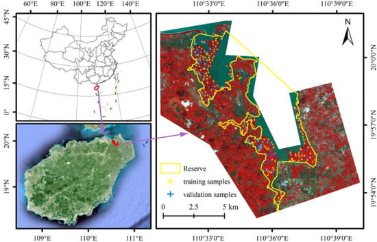
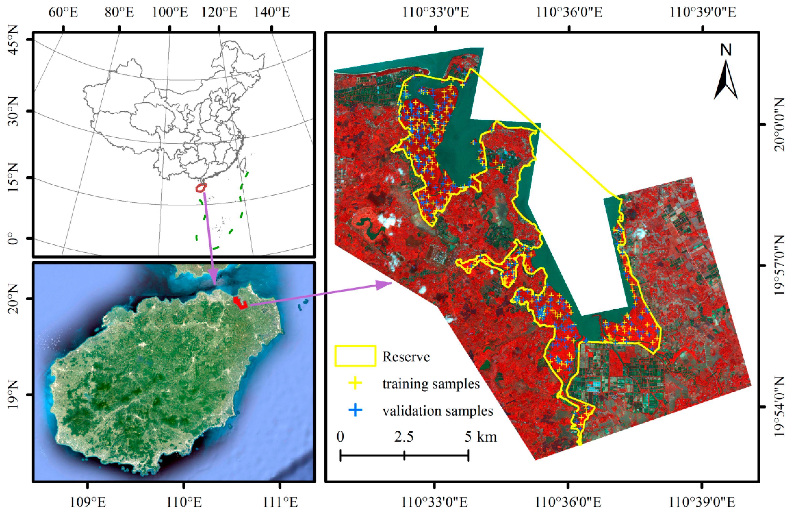
2.1. Study Area
2.2. Remote Sensing Data and Pre-Processing
2.3. Field Survey
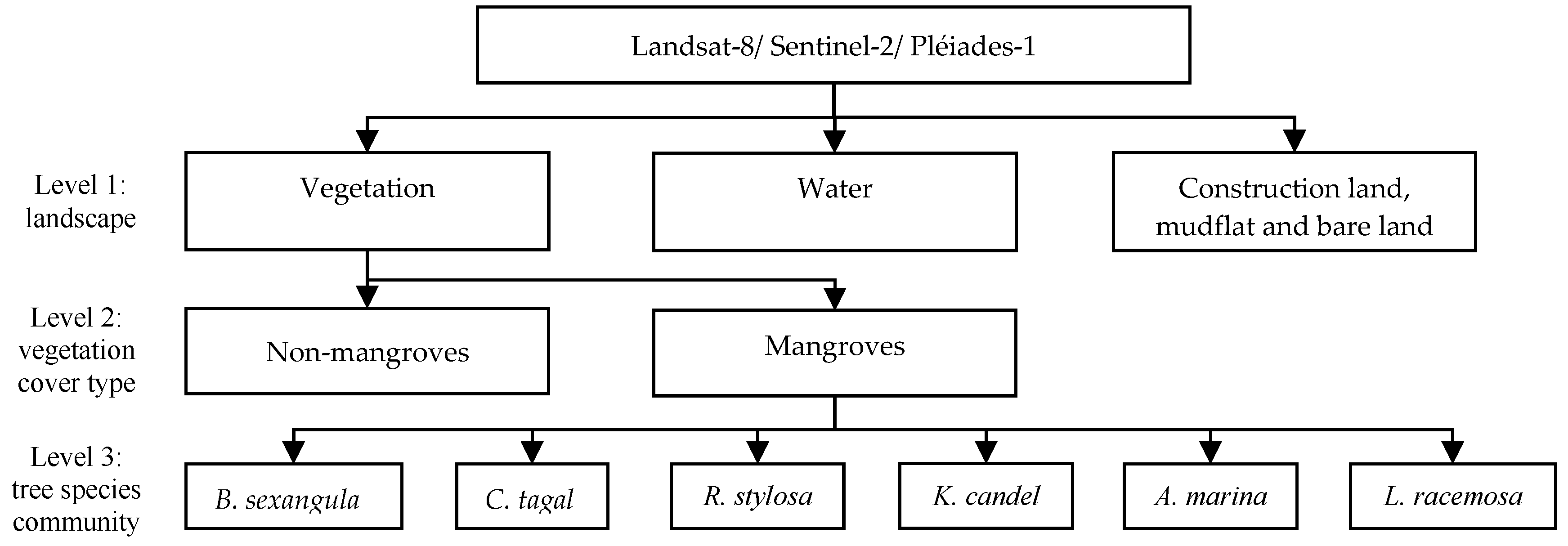
2.4. Two-Scale Mangrove Features Classifications
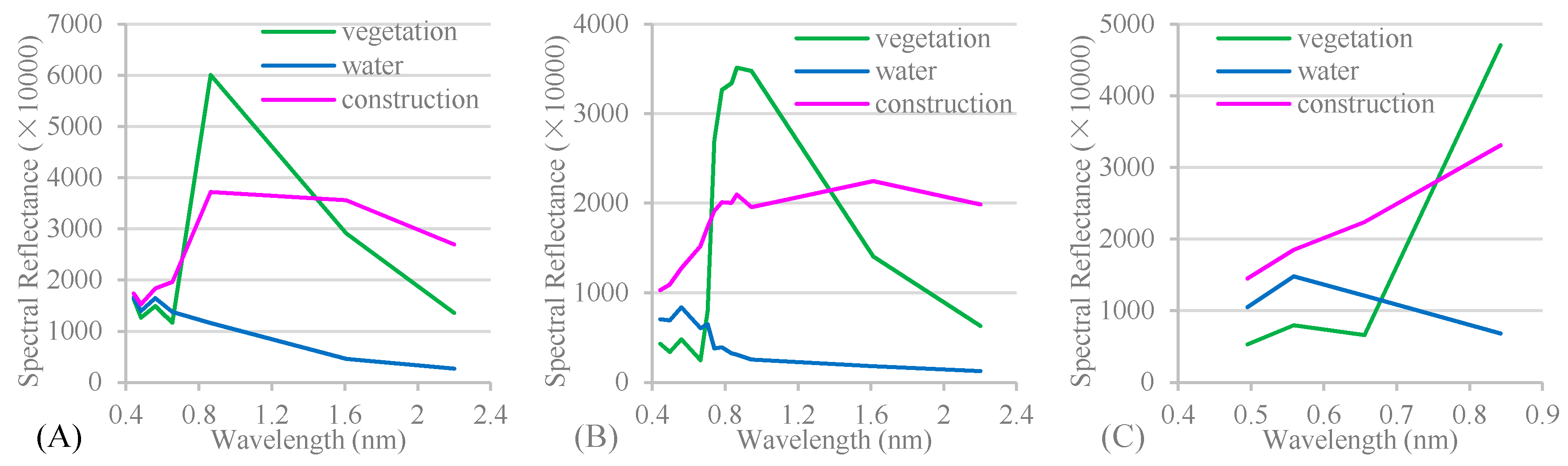
2.5. Spectral and Textural Features
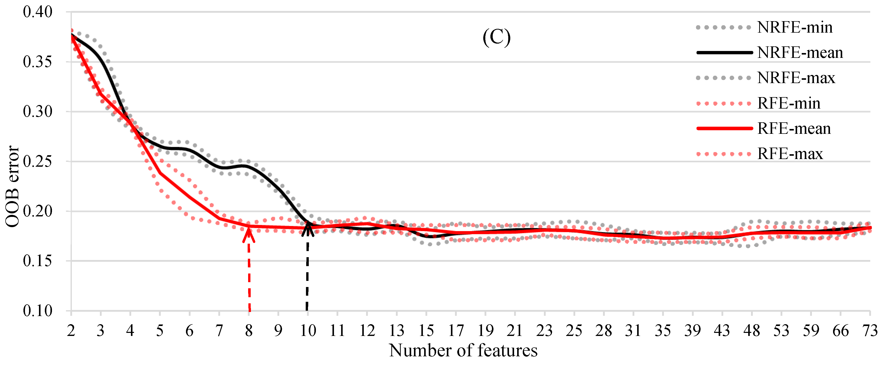
2.6. Random Forest Classification, Feature Selection and Parameters Tuning
- 1)
- Given the input predictor variables of size m, randomly permute the values of the ith (i = 1, 2, …, m) variable in the OOB samples;
- 2)
- Run the changed OOB data in the corresponding tree and obtain the errOOB 2 (OOB error 2), and the OOB error of the original data in the tree is named errOOB 1;
- 3)
- Repeat step (1) and (2) for all trees (ntree), and calculate the mean decrease accuracy (MDA) [53] for variable i by ;
- 4)
- Repeat step (1), (2), and (3) for each predictor variable and obtain its mean decrease accuracy.
2.7. Accuracy Assessment
3. Results
3.1. Mangrove and Non-Mangrove Classification
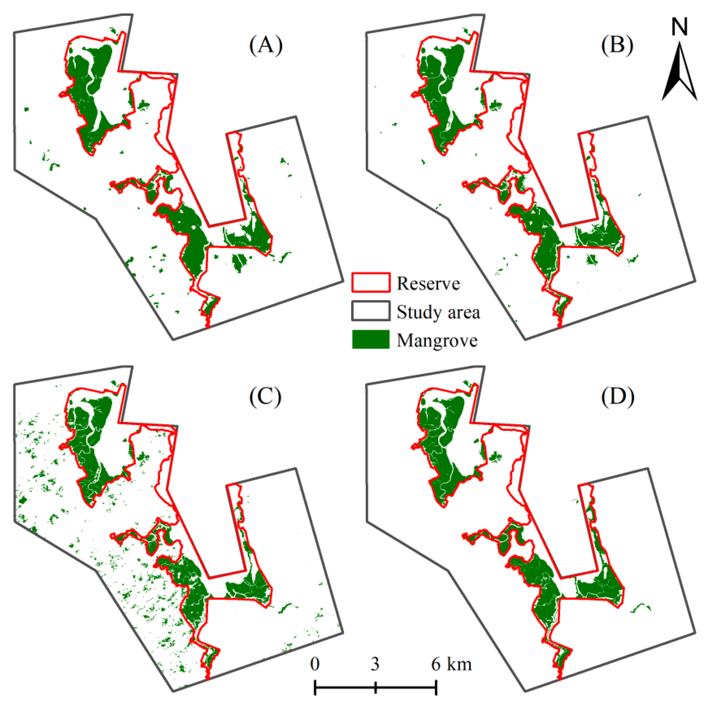
3.1.1. Visual Examination
3.1.2. Accuracy Assessment
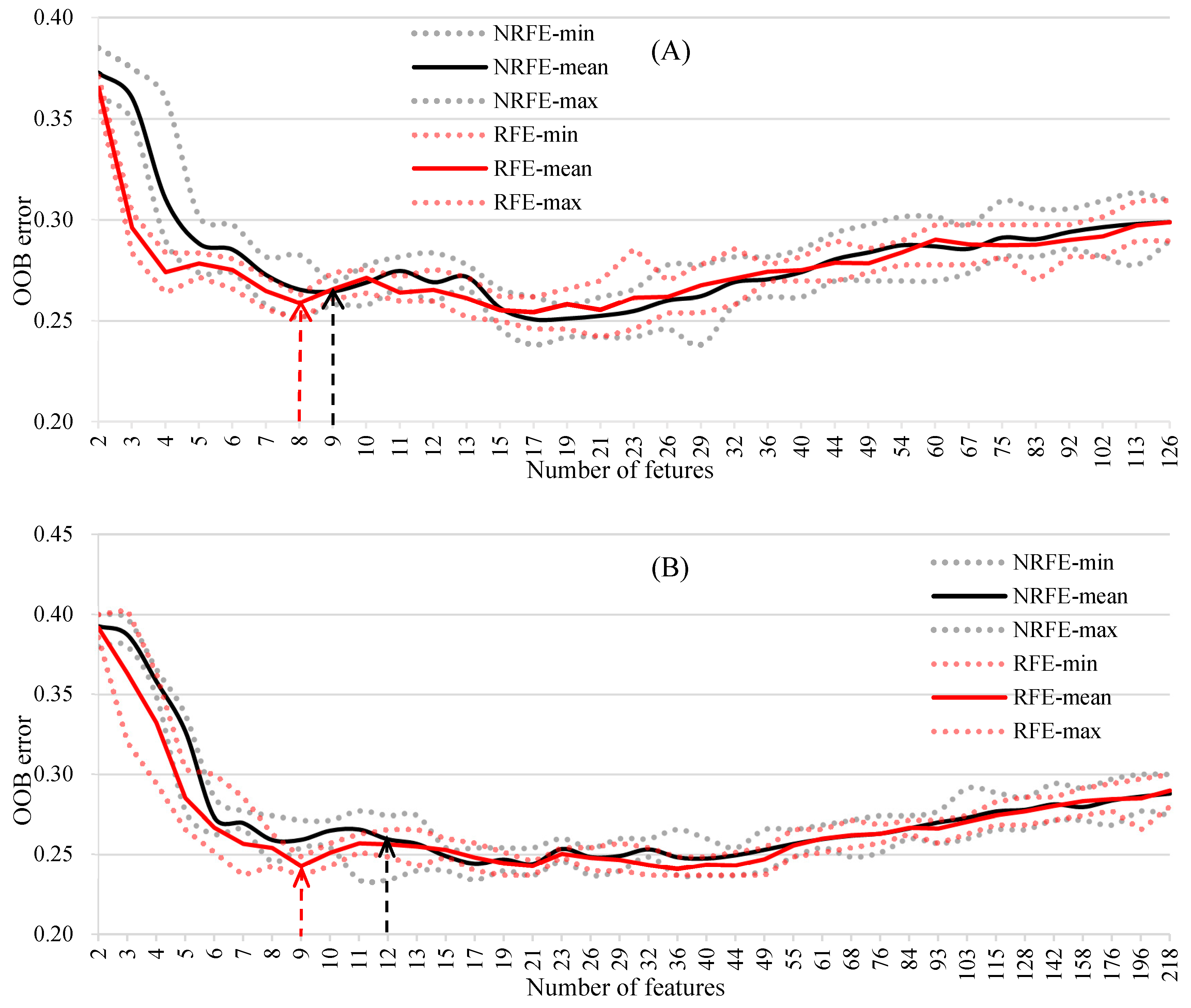
3.2. Object Feature Selection for the RF Model on Species Discrimination
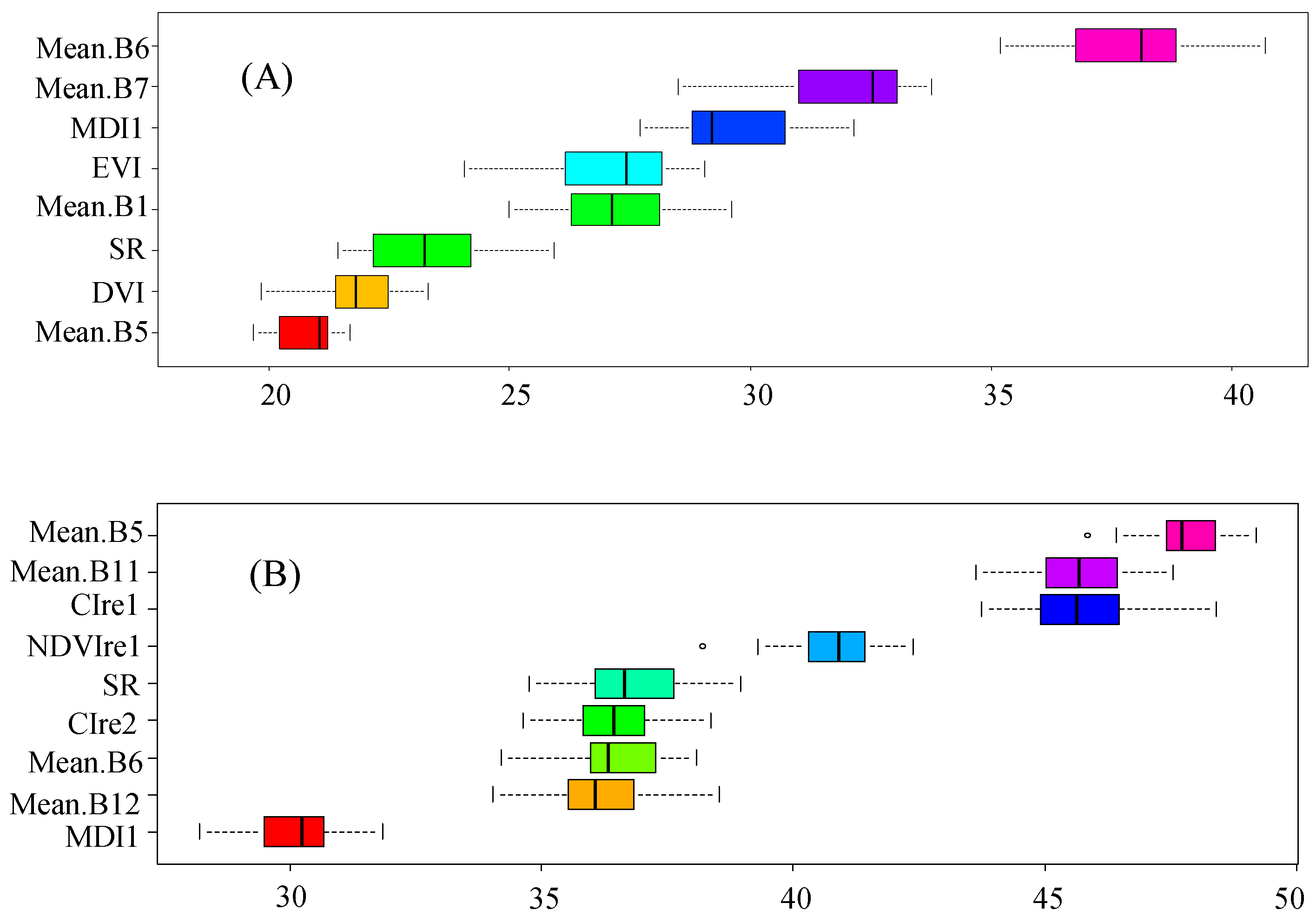
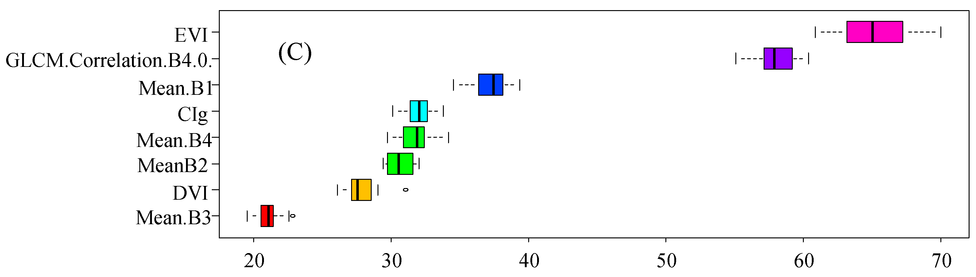
3.3. Feature Importance for Species Discrimination
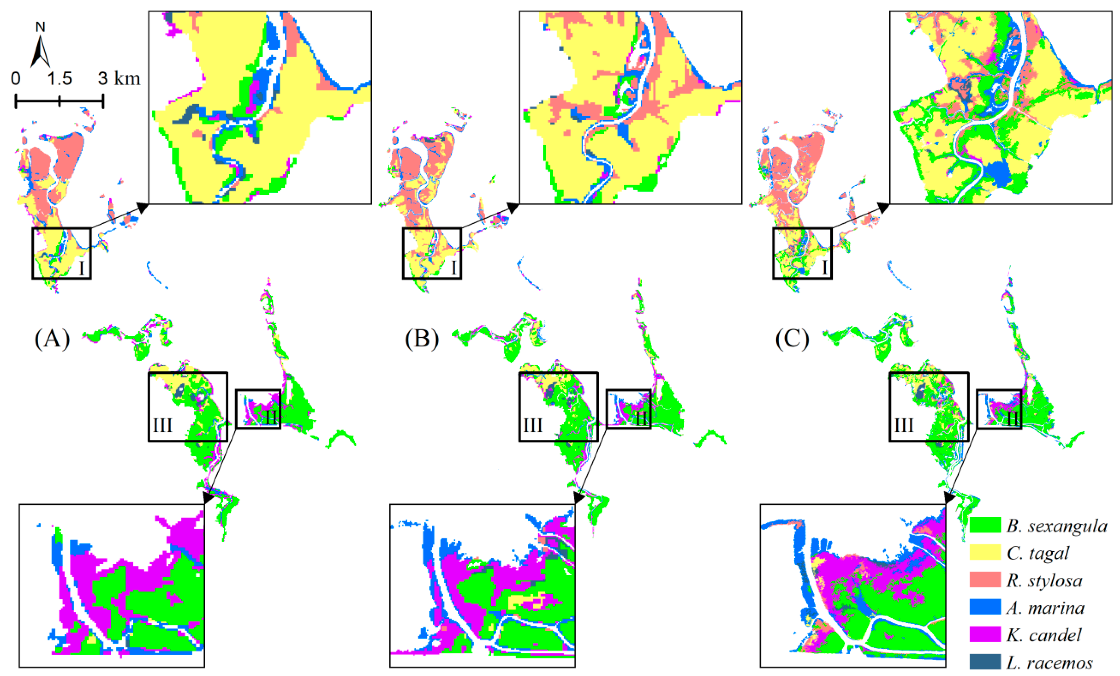
3.4. Mangrove Species Community Classification
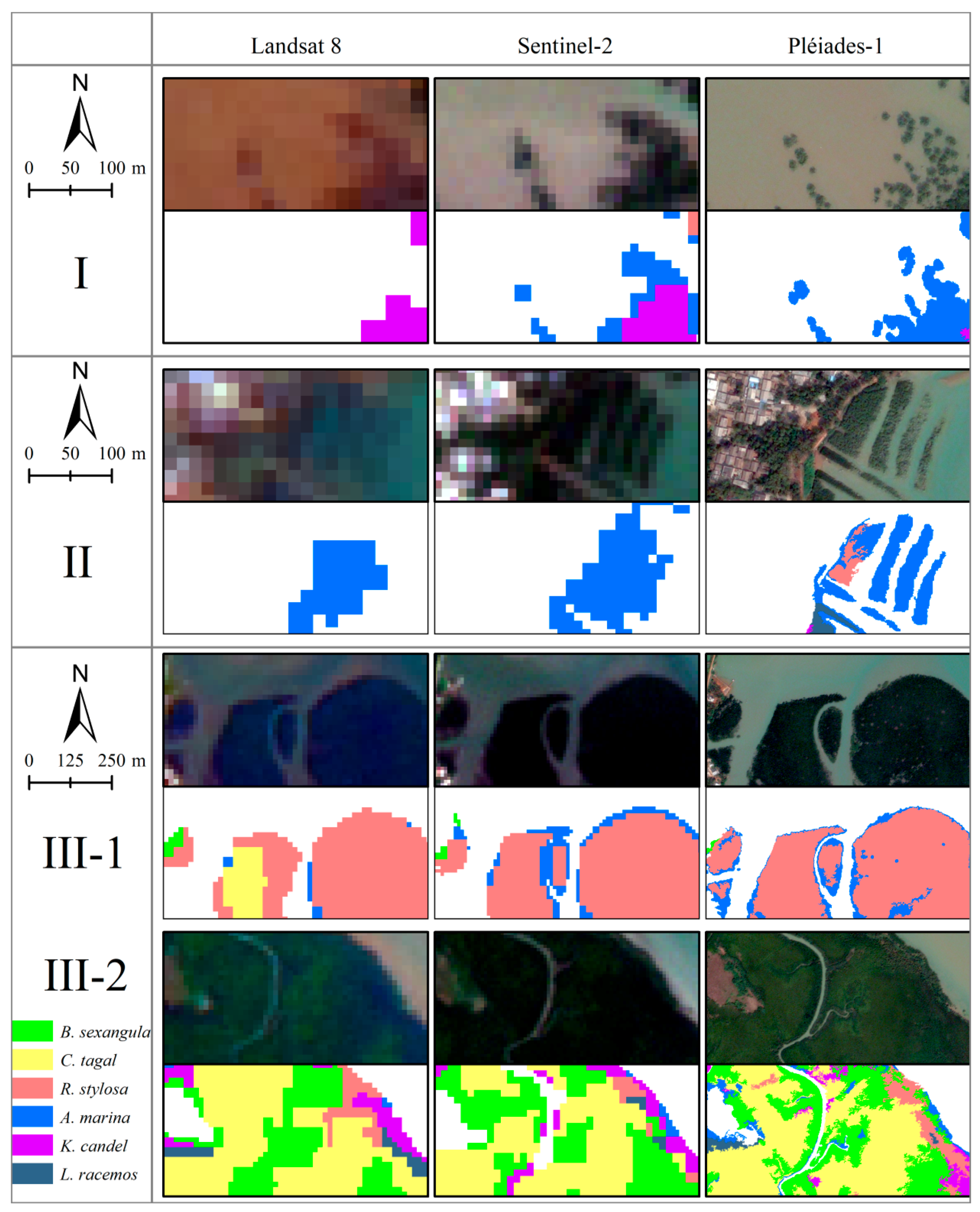
3.4.1. Visual Examination
3.4.2. Accuracy Assessment
4. Discussion
4.1. The Potential of Sentinel-2 Data for Mangrove Extent and Species Classifications
4.2. The Relationship between Spatial Resolutions and Mangrove Features
4.3. The Importance of Spectral Bands and Texture Information for Mangrove Classifications
4.4. The Superiority of Random Forests Classification
5. Conclusions
Author Contributions
Funding
Acknowledgments
Conflicts of Interest
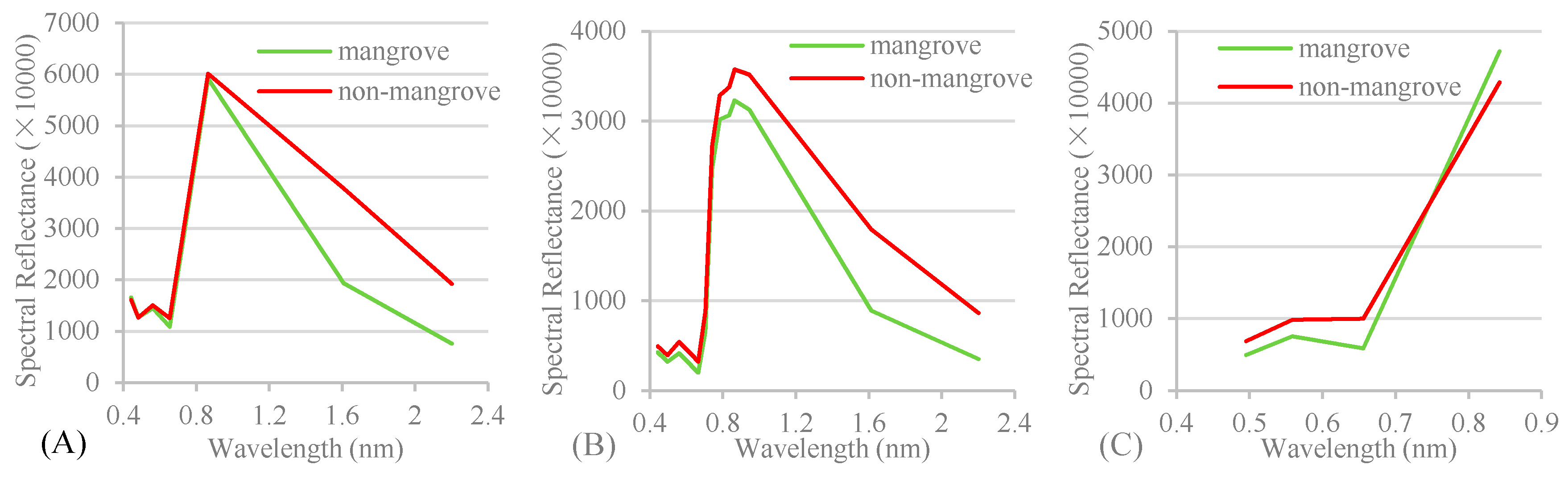
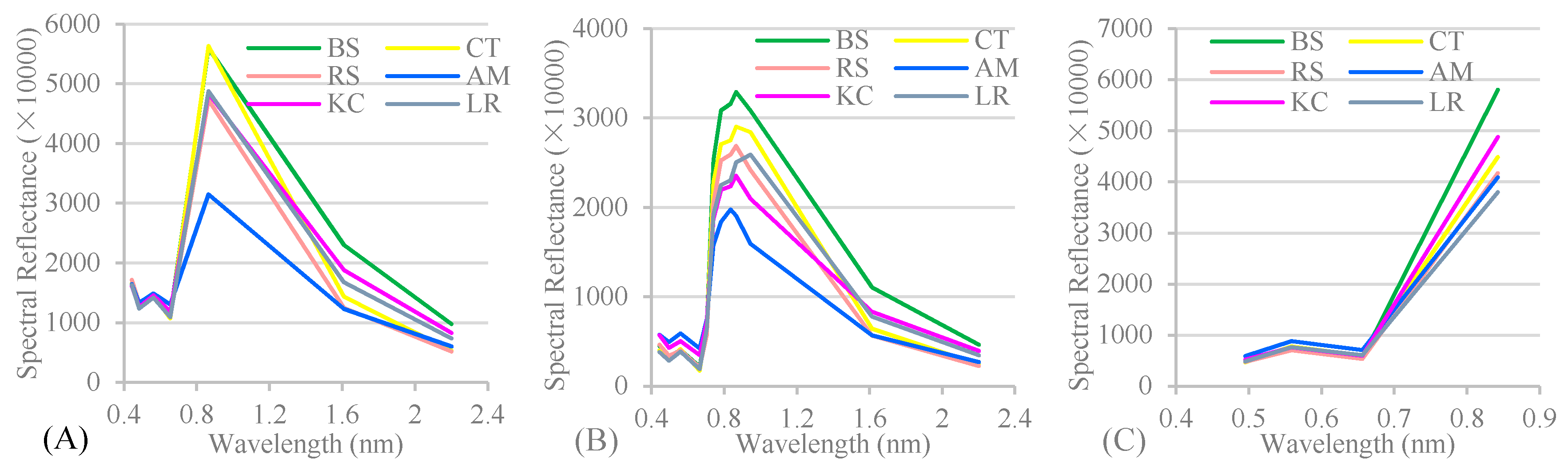
Appendix A. The spectral reflectance used in Level 1, Level 2 and Level 3


References
- Giri, C.; Ochieng, E.; Tieszen, L.L.; Zhu, Z.; Singh, A.; Loveland, T.; Masek, J.; Duke, N. Status and distribution of mangrove forests of the world using earth observation satellite data. Glob. Ecol. Biogeogr. 2011, 20, 154–159. [Google Scholar] [CrossRef]
- Giri, C. Observation and monitoring of mangrove forests using remote sensing: Opportunities and challenges. Remote Sens. 2016, 8, 783. [Google Scholar] [CrossRef]
- Duke, N.C.; Meynecke, J.O.; Dittmann, S.; Ellison, A.M.; Anger, K.; Berger, U.; Cannicci, S.; Diele, K.; Ewel, K.C.; Field, C.D. A world without mangroves? Science 2007, 317, 41. [Google Scholar] [CrossRef] [PubMed] [Green Version]
- Baowen, L.; Qiaomin, Z. Area, distribution and species composition of mangroves in china. Wetl. Sci. 2014, 12, 435–440. (In Chinese) [Google Scholar]
- Kuenzer, C.; Bluemel, A.; Gebhardt, S.; Tuan Vo, Q.; Dech, S. Remote sensing of mangrove ecosystems: A review. Remote Sens. 2011, 3, 878–928. [Google Scholar] [CrossRef]
- Heumann, B.W. Satellite remote sensing of mangrove forests: Recent advances and future opportunities. Prog. Phys. Geog. 2011, 35, 87–108. [Google Scholar] [CrossRef]
- Long, J.B.; Giri, C. Mapping the philippines’ mangrove forests using landsat imagery. Sensors 2011, 11, 2972–2981. [Google Scholar] [CrossRef] [PubMed]
- Jia, M.; Wang, Z.; Li, L.; Song, K.; Ren, C.; Liu, B.; Mao, D. Mapping china’s mangroves based on an object-oriented classification of landsat imagery. Wetlands 2014, 34, 277–283. [Google Scholar] [CrossRef]
- Mondal, P.; Trzaska, S.; de Sherbinin, A. Landsat-derived estimates of mangrove extents in the sierra leone coastal landscape complex during 1990–2016. Sensors 2018, 18, 12. [Google Scholar] [CrossRef] [PubMed]
- Kuenzer, C.; van Beijma, S.; Gessner, U.; Dech, S. Land surface dynamics and environmental challenges of the niger delta, africa: Remote sensing-based analyses spanning three decades (1986–2013). Appl. Geog. 2014, 53, 354–368. [Google Scholar] [CrossRef]
- Jia, M.M.; Liu, M.Y.; Wang, Z.M.; Mao, D.H.; Ren, C.Y.; Cui, H.S. Evaluating the effectiveness of conservation on mangroves: A remote sensing-based comparison for two adjacent protected areas in shenzhen and hong kong, china. Remote Sens. 2016, 8, 627. [Google Scholar] [CrossRef]
- Zhang, X.H.; Treitz, P.M.; Chen, D.M.; Quan, C.; Shi, L.X.; Li, X.H. Mapping mangrove forests using multi-tidal remotely-sensed data and a decision-tree-based procedure. Int. J. Appl. Earth. Obs. Geoinf. 2017, 62, 201–214. [Google Scholar] [CrossRef]
- Heenkenda, M.; Joyce, K.; Maier, S.; Bartolo, R. Mangrove species identification: Comparing worldview-2 with aerial photographs. Remote Sens. 2014, 6, 6064–6088. [Google Scholar] [CrossRef]
- Wang, T.; Zhang, H.; Lin, H.; Fang, C. Textural–spectral feature-based species classification of mangroves in mai po nature reserve from worldview-3 imagery. Remote Sens. 2016, 8, 24. [Google Scholar] [CrossRef]
- Dezhi, W.; Bo, W.; Penghua, Q.; Yanjun, S.; Qinghua, G.; Xincai, W. Artificial mangrove species mapping using pléiades-1: An evaluation of pixel-based and object-based classifications with selected machine learning algorithms. Remote Sens. 2018, 10, 294. [Google Scholar]
- Castillo, J.A.A.; Apan, A.A.; Maraseni, T.N.; Salmo, S.G. Estimation and mapping of above-ground biomass of mangrove forests and their replacement land uses in the philippines using sentinel imagery. ISPRS J. Photogramm. Remote Sens. 2017, 134, 70–85. [Google Scholar] [CrossRef]
- Zhu, Y.; Liu, K.; Liu, L.; Myint, S.; Wang, S.; Liu, H.; He, Z. Exploring the potential of worldview-2 red-edge band-based vegetation indices for estimation of mangrove leaf area index with machine learning algorithms. Remote Sens. 2017, 9, 1060. [Google Scholar] [CrossRef]
- Chen, B.Q.; Xiao, X.M.; Li, X.P.; Pan, L.H.; Doughty, R.; Ma, J.; Dong, J.W.; Qin, Y.W.; Zhao, B.; Wu, Z.X.; et al. A mangrove forest map of china in 2015: Analysis of time series landsat 7/8 and sentinel-1a imagery in google earth engine cloud computing platform. ISPRS J. Photogramm. Remote Sens. 2017, 131, 104–120. [Google Scholar] [CrossRef]
- Leon, T.; Giang, V.; An, B.; Minh, N.; Quynh, N.T.; Le, Q.; Viet, P. Uncovering the spatio-temporal dynamics of land cover change and fragmentation of mangroves in the ca mau peninsula, vietnam using multi-temporal spot satellite imagery (2004–2013). Appl. Geog. 2017, 86, 197–207. [Google Scholar]
- Wang, L.; Sousa, W.P.; Peng, G.; Biging, G.S. Comparison of ikonos and quickbird images for mapping mangrove species on the caribbean coast of panama. Remote Sens. Environ. 2004, 91, 432–440. [Google Scholar] [CrossRef]
- Pham, L.T.H.; Brabyn, L. Monitoring mangrove biomass change in vietnam using spot images and an object-based approach combined with machine learning algorithms. ISPRS J. Photogramm. Remote Sens. 2017, 128, 86–97. [Google Scholar] [CrossRef]
- Drusch, M.; Bello, U.D.; Carlier, S.; Colin, O.; Fernandez, V.; Gascon, F.; Hoersch, B.; Isola, C.; Laberinti, P.; Martimort, P. Sentinel-2: Esa’s optical high-resolution mission for gmes operational services. Remote Sens. Environ. 2012, 120, 25–36. [Google Scholar] [CrossRef]
- Immitzer, M.; Vuolo, F.; Atzberger, C. First experience with sentinel-2 data for crop and tree species classifications in central europe. Remote Sens. 2016, 8, 166. [Google Scholar] [CrossRef]
- Korhonen, L.; Hadi; Packalen, P.; Rautiainen, M. Comparison of sentinel-2 and landsat 8 in the estimation of boreal forest canopy cover and leaf area index. Remote Sens. Environ. 2017, 195, 259–274. [Google Scholar] [CrossRef]
- Shoko, C.; Mutanga, O. Examining the strength of the newly-launched sentinel 2 msi sensor in detecting and discriminating subtle differences between c3 and c4 grass species. ISPRS J. Photogramm. Remote Sens. 2017, 129, 32–40. [Google Scholar] [CrossRef]
- Mura, M.; Bottalico, F.; Giannetti, F.; Bertani, R.; Giannini, R.; Mancini, M.; Orlandini, S.; Travaglini, D.; Chirici, G. Exploiting the capabilities of the sentinel-2 multi spectral instrument for predicting growing stock volume in forest ecosystems. Int. J. Appl. Earth. Obs. Geoinf. 2018, 66, 126–134. [Google Scholar] [CrossRef]
- Puliti, S.; Saarela, S.; Gobakken, T.; Stahl, G.; Naesset, E. Combining uav and sentinel-2 auxiliary data for forest growing stock volume estimation through hierarchical model-based inference. Remote Sens. Environ. 2018, 204, 485–497. [Google Scholar] [CrossRef]
- Shapiro, A.; Trettin, C.; Küchly, H.; Alavinapanah, S.; Bandeira, S. The mangroves of the zambezi delta: Increase in extent observed via satellite from 1994 to 2013. Remote Sens. 2015, 7, 16504–16518. [Google Scholar] [CrossRef]
- Pastor-Guzman, J.; Atkinson, P.; Dash, J.; Rioja-Nieto, R. Spatiotemporal variation in mangrove chlorophyll concentration using landsat 8. Remote Sens. 2015, 7, 14530–14558. [Google Scholar] [CrossRef]
- Valderrama-Landeros, L.; Flores-de-Santiago, F.; Kovacs, J.M.; Flores-Verdugo, F. An assessment of commonly employed satellite-based remote sensors for mapping mangrove species in mexico using an ndvi-based classification scheme. Environ. Monit. Assess. 2018, 190, 13. [Google Scholar] [CrossRef] [PubMed]
- Asian, A.; Rahman, A.F.; Warren, M.W.; Robeson, S.M. Mapping spatial distribution and biomass of coastal wetland vegetation in indonesian papua by combining active and passive remotely sensed data. Remote Sens. Environ. 2016, 183, 65–81. [Google Scholar]
- Almahasheer, H. Spatial coverage of mangrove communities in the arabian gulf. Environ. Monit. Assess. 2018, 190, 10. [Google Scholar] [CrossRef] [PubMed]
- Abd-El Monsef, H.; Smith, S.E. A new approach for estimating mangrove canopy cover using landsat 8 imagery. Comput. Electron. Agric. 2017, 135, 183–194. [Google Scholar] [CrossRef]
- Wicaksono, P. Mangrove above-ground carbon stock mapping of multi-resolution passive remote-sensing systems. Int. J. Remote Sens. 2017, 38, 1551–1578. [Google Scholar] [CrossRef]
- Hickey, S.M.; Callow, N.J.; Phinn, S.; Lovelock, C.E.; Duarte, C.M. Spatial complexities in aboveground carbon stocks of a semi-arid mangrove community: A remote sensing height-biomass-carbon approach. Estuar. Coast. Shelf Sci. 2018, 200, 194–201. [Google Scholar] [CrossRef]
- Cardenas, N.Y.; Joyce, K.E.; Maier, S.W. Monitoring mangrove forests: Are we taking full advantage of technology? Int. J. Appl. Earth. Obs. Geoinf. 2017, 63, 1–14. [Google Scholar] [CrossRef]
- Song, C.; Woodcock, C.E.; Seto, K.C.; Lenney, M.P.; Macomber, S.A. Classification and change detection using landsat tm data: When and how to correct atmospheric effects? Remote Sens. Environ. 2001, 75, 230–244. [Google Scholar] [CrossRef]
- Sun, W.; Messinger, D. Nearest-neighbor diffusion-based pan-sharpening algorithm for spectral images. Opt. Eng. 2013, 53, 013107. [Google Scholar] [CrossRef]
- Xin, K.; Yan, K.; Gao, C.; Li, Z. Carbon storage and its influencing factors in hainan dongzhangang mangrove wetlands. Mar. Freshwater Res. 2018, 69, 771–779. [Google Scholar] [CrossRef]
- Kamal, M.; Phinn, S.; Johansen, K. Object-based approach for multi-scale mangrove composition mapping using multi-resolution image datasets. Remote Sens. 2015, 7, 4753–4783. [Google Scholar] [CrossRef]
- Baatz, M.; Schape, A. Multiresolution segmentation: An optimization approach for high quality multi-scale image segmentation. In Angewandte Geographische Information Sverarbeitung XII; Herbert Wichmann Verlag: Karhlsruhe, Germany, 2000; pp. 12–23. [Google Scholar]
- Duro, D.C.; Franklin, S.E.; Dubé, M.G. A comparison of pixel-based and object-based image analysis with selected machine learning algorithms for the classification of agricultural landscapes using spot-5 hrg imagery. Remote Sens. Environ. 2012, 118, 259–272. [Google Scholar] [CrossRef]
- Ji, L.; Zhang, L.; Wylie, B. Analysis of dynamic thresholds for the normalized difference water index. Photogramm. Eng. Remote Sens. 2009, 75, 1307–1317. [Google Scholar] [CrossRef]
- Drăguţ, L.; Csillik, O.; Eisank, C.; Tiede, D. Automated parameterisation for multi-scale image segmentation on multiple layers. ISPRS J. Photogramm. Remote Sens. 2014, 88, 119–127. [Google Scholar] [CrossRef] [PubMed]
- Zhu, Y.; Liu, K.; Liu, L.; Wang, S.; Liu, H. Retrieval of mangrove aboveground biomass at the individual species level with worldview-2 images. Remote Sens. 2015, 7, 12192–12214. [Google Scholar] [CrossRef]
- Wicaksono, P.; Danoedoro, P.; Hartono; Nehren, U. Mangrove biomass carbon stock mapping of the karimunjawa islands using multispectral remote sensing. Int. J. Remote Sens. 2016, 37, 26–52. [Google Scholar] [CrossRef]
- Fernandez-Manso, A.; Fernandez-Manso, O.; Quintano, C. Sentinel-2a red-edge spectral indices suitability for discriminating burn severity. Int. J. Appl. Earth. Obs. Geoinf. 2016, 50, 170–175. [Google Scholar] [CrossRef]
- Gitelson, A.A.; Gritz, Y.; Merzlyak, M.N. Relationships between leaf chlorophyll content and spectral reflectance and algorithms for non-destructive chlorophyll assessment in higher plant leaves. J. Plant. Physiol. 2003, 160, 271–282. [Google Scholar] [CrossRef] [PubMed]
- Haralick, R.M.; Shanmugam, K.; Dinstein, I.H. Textural features for image classification. IEEE Trans. Syst. Man. Cybern. 1973, 3, 610–621. [Google Scholar] [CrossRef]
- Belgiu, M.; Dragut, L. Random forest in remote sensing: A review of applications and future directions. ISPRS J. Photogramm. Remote Sens. 2016, 114, 24–31. [Google Scholar] [CrossRef]
- Breiman, L. Random forests. Mach. Learn. 2001, 45, 5–32. [Google Scholar] [CrossRef]
- Li, M.; Ma, L.; Blaschke, T.; Cheng, L.; Tiede, D. A systematic comparison of different object-based classification techniques using high spatial resolution imagery in agricultural environments. Int. J. Appl. Earth Obs. Geoinf. 2016, 49, 87–98. [Google Scholar] [CrossRef]
- Genuer, R.; Poggi, J.M.; Tuleau-Malot, C. Variable selection using random forests. Pattern Recognit. Lett. 2010, 31, 2225–2236. [Google Scholar] [CrossRef] [Green Version]
- Gregorutti, B.; Michel, B.; Saint-Pierre, P. Correlation and variable importance in random forests. Stat. Comput. 2017, 27, 659–678. [Google Scholar] [CrossRef]
- Li, X.; Chen, W.; Cheng, X.; Wang, L. A comparison of machine learning algorithms for mapping of complex surface-mined and agricultural landscapes using ziyuan-3 stereo satellite imagery. Remote Sens. 2016, 8, 514. [Google Scholar] [CrossRef]
- Ng, W.-T.; Rima, P.; Einzmann, K.; Immitzer, M.; Atzberger, C.; Eckert, S. Assessing the potential of sentinel-2 and pléiades data for the detection of prosopis and vachellia spp. In kenya. Remote Sens. 2017, 9, 74. [Google Scholar] [CrossRef]
- Rodriguez-Galiano, V.F.; Ghimire, B.; Rogan, J.; Chica-Olmo, M.; Rigol-Sanchez, J.P. An assessment of the effectiveness of a random forest classifier for land-cover classification. ISPRS J. Photogramm. 2012, 67, 93–104. [Google Scholar] [CrossRef]
- Foody, G.M. Sample size determination for image classification accuracy assessment and comparison. Int. J. Remote Sens. 2009, 30, 5273–5291. [Google Scholar] [CrossRef]
- Kamal, M.; Phinn, S.; Johansen, K. Characterizing the spatial structure of mangrove features for optimizing image-based mangrove mapping. Remote Sens. 2014, 6, 984–1006. [Google Scholar] [CrossRef]
- Heumann, B.W. An object-based classification of mangroves using a hybrid decision tree—support vector machine approach. Remote Sens. 2011, 3, 2440–2460. [Google Scholar] [CrossRef]
- Shi, T.Z.; Liu, J.; Hu, Z.W.; Liu, H.Z.; Wang, J.J.; Wu, G.F. New spectral metrics for mangrove forest identification. Remote Sens. Lett. 2016, 7, 885–894. [Google Scholar] [CrossRef]
- Wang, L.; Sousa, W.P. Distinguishing mangrove species with laboratory measurements of hyperspectral leaf reflectance. Int. J. Remote Sens. 2009, 30, 1267–1281. [Google Scholar] [CrossRef]
- Puissant, A.; Rougier, S.; Stumpf, A. Object-oriented mapping of urban trees using random forest classifiers. Int. J. Appl. Earth. Obs. Geoinf. 2014, 26, 235–245. [Google Scholar] [CrossRef]
- Pelletier, C.; Valero, S.; Inglada, J.; Champion, N.; Dedieu, G. Assessing the robustness of random forests to map land cover with high resolution satellite image time series over large areas. Int. J. Remote Sens. 2016, 187, 156–168. [Google Scholar] [CrossRef]
- Colditz, R.R. An evaluation of different training sample allocation schemes for discrete and continuous land cover classification using decision tree-based algorithms. Remote Sens. 2015, 7, 9655–9681. [Google Scholar] [CrossRef]
- Tolosi, L.; Lengauer, T. Classification with correlated features: Unreliability of feature ranking and solutions. Bioinformatics 2011, 27, 1986–1994. [Google Scholar] [CrossRef] [PubMed]


| Spectrum | Landsat 8 2016-2-14 | Sentinel-2A 2016-12-9 | Pléiades-1B 2014-2-4 | |||||||||
|---|---|---|---|---|---|---|---|---|---|---|---|---|
| Band | Centre (nm) | Wave Width (nm) | Spatial Resolution (m) | Band | Centre (nm) | Wave Width (nm) | Spatial Resolution (m) | Band | Centre (nm) | Wave Width (nm) | Spatial Resolution (m) | |
| Aerosol | B1 | 443 | 16 | 30 | B1 | 442.3 | 45 | 60 | ||||
| Blue | B2 | 482.6 | 60.1 | 30 | B2 | 492.1 | 98 | 10 | B1 | 495 | 76.5 | 2 |
| Green | B3 | 561.3 | 57.4 | 30 | B3 | 559 | 46 | 10 | B2 | 558.5 | 83.7 | 2 |
| Pan | B8 | 591.7 | 172.4 | 15 | - | - | - | - | B5 | 652.5 | 326.8 | 0.5 |
| Red | B4 | 654.6 | 37.5 | 30 | B4 | 665 | 39 | 10 | B3 | 656 | 78.8 | 2 |
| Red edge-1 | - | - | - | - | B5 | 703.8 | 20 | 20 | - | - | - | - |
| Red edge-2 | - | - | - | - | B6 | 739.1 | 18 | 20 | - | - | - | - |
| Red edge-3 | - | - | - | - | B7 | 779.7 | 28 | 20 | - | - | - | - |
| NIR | - | - | - | - | B8 | 833 | 133 | 10 | - | - | - | - |
| NIR | B5 | 864.6 | 28.2 | 30 | B8a | 864 | 32 | 20 | B4 | 842.5 | 130.3 | 2 |
| Water vapor | - | - | - | - | B9 | 943.2 | 27 | 60 | - | - | - | - |
| Cirrus | B9 | 1373 | 20.4 | 30 | B10 | 1376.9 | 76 | 60 | - | - | - | - |
| SWIR-1 | B6 | 1609 | 84.7 | 30 | B11 | 1610.4 | 141 | 20 | - | - | - | - |
| SWIR-2 | B7 | 2201 | 186.7 | 30 | B12 | 2185.7 | 238 | 20 | - | - | - | - |
| Species | Training Samples (Average Area about 1000 m2, Min Area ≥300 m2) | Validation Samples (Center Point) |
|---|---|---|
| Bruguiera sexangula | 55 | 48 |
| Ceriops tagal | 55 | 48 |
| Rhizophora stylosa | 55 | 48 |
| Kandelia candel | 25 | 22 |
| Avicennia marina | 25 | 22 |
| Lumnitzera racemosa | 25 | 22 |
| Sum | 240 | 210 |
| Level | Landsat 8 15 m | Sentinel-2 10 m | Pléiades-1 0.5 m | |
|---|---|---|---|---|
| Level 1 | water | Chessboard Seg: 1 MNDWI > 0 FDI < 0 | Chessboard Seg: 1 MNDWI > 0 FDI < 0 Brightness < 1250 | Multiresolution Seg: 500 NDWI ≥ −0.25 Brightness < 2000 |
| vegetation | WFI > 1.2 | WFI > 0.7 | NDVI > 0.4 | |
| Construction land, mudflat and bare land | Not “Vegetation” or “Water” | Not “Vegetation” or “Water” | Not “Vegetation” or “Water” | |
| Level 2 | Mangrove | Multiresolution Seg: 80 MDI2 > 3.4 | Multiresolution Seg: 64 MDI2 > 4.7 | Multiresolution Seg: 500 300 < Red < 660 4200 < NIR < 6000 |
| Non-mangrove | Not “Mangroves” | Not “Mangroves” | Not “Mangroves” | |
| Level 3 | Mangrove species community | Multiresolution Seg: 30 Random Forest in R | Multiresolution Seg: 30 Random Forest in R | Multiresolution Seg: 350 Random Forest in R |
| Object Features | Formula for Landsat 8 | Formula for Sentinel-2 | Formula for Pléiades-1 | Reference | |
|---|---|---|---|---|---|
| Spectral Bands | Individual Bands | B1, B2, B3, B4, B5, B6, B7 | B1, B2, B3, B4, B5, B6, B7, B8, B8a, B9, B11, B12 | B1, B2, B3, B4 | NA |
| Conventional NIR indices | DVI | B5 − B4 | B8 − B4 | B4 − B3 | [45] |
| CIg | (B5/B3) − 1 | (B8/B3) − 1 | (B4/B2) − 1 | [48] | |
| SR | B5/B4 | B8/B4 | B4/B3 | [45] | |
| NDVI | (B5 − B4)/(B5 + B4) | (B8 − B4)/(B8 + B4) | (B4 − B3)/(B4 + B3) | [46] | |
| EVI | [24] | ||||
| Red edge indices | CIre1 | NA | B5/B3-1 | NA | [47] |
| CIre2 | NA | B6/B3-1 | NA | [47] | |
| CIre3 | NA | B7/B3-1 | NA | [47] | |
| NDVIre1 | NA | (B8 − B5)/(B8 + B5) | NA | [25] | |
| NDVIre2 | NA | (B8 − B6)/(B8 + B6) | NA | [25] | |
| NDVIre3 | NA | (B8 − B7)/(B8 + B7) | NA | [25] | |
| MSRren | NA | NA | [47] | ||
| Shortwave infrared indices | MDI1 | (B5 − B6)/B6 | (B8 − B11)/B11 | NA | NA |
| MDI2 | (B5 − B7)/B7 | (B8 − B12)/B12 | NA | NA | |
| Texture information | Homogeneity | the same to left | the same to left | [14] | |
| Contrast | the same to left | the same to left | [14] | ||
| Entropy | the same to left | the same to left | [14] | ||
| Correlation | the same to left | the same to left | [14] | ||
| NRFE | RFE |
|---|---|
| 1. Train an initial random forest model, and rank the features using the permutation importance measure | 1. Train a random forest model |
| 2. Eliminate the less relevant feature(s) | 2. Compute the permutation importance measure |
| 3. Train a random forest model | 3. Eliminate the less relevant feature(s) |
| 4. Repeat steps 2 and 3 until no further features remain | 4. Repeat steps 1–3 until no further features remain |
| Classifier A | |||
|---|---|---|---|
| Correct | Incorrect | ||
| Classifier B | Correct | 11 | 12 |
| Incorrect | 21 | 22 | |
| Class | Landsat 8, 15 m | Sentinel-2, 10 m | Pléiades-1, 0.5 m | |||||||||
|---|---|---|---|---|---|---|---|---|---|---|---|---|
| Pa | Ua | Oa | K | Pa | Ua | Oa | K | Pa | Ua | Oa | K | |
| Mangrove | 92.66 | 89.38 | 96.09 | 0.93 | 90.29 | 92.08 | 96.52 | 0.94 | 94.17 | 72.93 | 91.89 | 0.87 |
| Non-mangrove | 97.02 | 97.99 | 98.07 | 97.60 | 91.33 | 98.44 | ||||||
| Class | Landsat 8 | Sentinel-2 | Pléiades-1 | |||||||||
|---|---|---|---|---|---|---|---|---|---|---|---|---|
| Pa (%) | Ua (%) | Oa (%) | K | Pa (%) | Ua (%) | Oa (%) | K | Pa (%) | Ua (%) | Oa (%) | K | |
| B. sexangula | 75.00 | 66.67 | 68.57 | 0.66 | 81.25 | 68.42 | 70.95 | 0.68 | 93.75 | 73.77 | 78.57 | 0.76 |
| C. tagal | 60.42 | 63.04 | 66.67 | 68.09 | 66.67 | 74.42 | ||||||
| R. stylosa | 79.17 | 79.17 | 83.33 | 75.47 | 85.42 | 83.67 | ||||||
| K. candel | 50.00 | 52.38 | 40.91 | 50.00 | 45.45 | 66.67 | ||||||
| A. marina | 72.27 | 66.67 | 50.00 | 78.57 | 77.27 | 85.00 | ||||||
| L. racemosa | 63.64 | 82.35 | 81.82 | 85.71 | 90.91 | 90.91 | ||||||
| McNemar’s Test chi-Square | p-Value | |
|---|---|---|
| Sentinel-2 vs. Landsat 8 | 0.3636 | 0.54650 |
| Sentinel-2 vs. Pléiades-1 | 4.7407 * | 0.02946 * |
| Landsat 8 vs. Pléiades-1 | 8.3333 * | 0.00389 * |
© 2018 by the authors. Licensee MDPI, Basel, Switzerland. This article is an open access article distributed under the terms and conditions of the Creative Commons Attribution (CC BY) license (http://creativecommons.org/licenses/by/4.0/).
Share and Cite
Wang, D.; Wan, B.; Qiu, P.; Su, Y.; Guo, Q.; Wang, R.; Sun, F.; Wu, X. Evaluating the Performance of Sentinel-2, Landsat 8 and Pléiades-1 in Mapping Mangrove Extent and Species. Remote Sens. 2018, 10, 1468. https://doi.org/10.3390/rs10091468
Wang D, Wan B, Qiu P, Su Y, Guo Q, Wang R, Sun F, Wu X. Evaluating the Performance of Sentinel-2, Landsat 8 and Pléiades-1 in Mapping Mangrove Extent and Species. Remote Sensing. 2018; 10(9):1468. https://doi.org/10.3390/rs10091468
Chicago/Turabian StyleWang, Dezhi, Bo Wan, Penghua Qiu, Yanjun Su, Qinghua Guo, Run Wang, Fei Sun, and Xincai Wu. 2018. "Evaluating the Performance of Sentinel-2, Landsat 8 and Pléiades-1 in Mapping Mangrove Extent and Species" Remote Sensing 10, no. 9: 1468. https://doi.org/10.3390/rs10091468