Harnessing the Temporal Dimension to Improve Object-Based Image Analysis Classification of Wetlands

Abstract

Research related to object-based image analysis has typically relied on data inputs that provide information on the spectral and spatial characteristics of objects, but the temporal domain is far less explored. For some objects, which are spectrally similar to other landscape features, their temporal pattern may be their sole defining characteristic. When multiple images are used in object-based image analysis, it is often constrained to a specific number of images which are selected because they cover the perceived range of temporal variability of the features of interest. Here, we provide a method to identify wetlands using a time series of Landsat imagery by building a Random Forest model using each image observation as an explanatory variable. We tested our approach in Douglas County, Washington, USA. Our approach exploiting the temporal domain classified wetlands with a high level of accuracy and reduced the number of spectrally similar false positives. We explored how sampling design (i.e., random, stratified, purposive) and temporal resolution (i.e., number of image observations) affected classification accuracy. We found that sampling design introduced bias in different ways, but did not have a substantial impact on overall accuracy. We also found that a higher number of image observations up to a point improved classification accuracy dependent on the selection of images used in the model. While time series analysis has been part of pixel-based remote sensing for many decades, with improved computer processing and increased availability of time series datasets (e.g., Landsat archive), it is now much easier to incorporate time series into object-based image analysis classification.

1. Introduction

Object-based image analysis (OBIA) is a remote sensing technique used to identify and classify objects through a process of pattern recognition [1]. OBIA differs from pixel-based techniques by aggregating raster pixels with similar characteristics into segments or objects [1]. Once an image raster is segmented, the objects can be classified using analyst-defined rules, machine learning techniques, or statistical methods. Because the object no longer consists of a single pixel, additional features such as shape, size, and context—not just the spectral features—can be used to drive the classification. Object-based approaches are commonly used on high spatial resolution data with limited spectral bands (e.g., red, blue, and green) where traditional pixel-based approaches are less effective [2]. Often, additional raster or vector layers, such as road layers, slope indices, and soil data, are added to provide additional variables to help characterize objects. For a good review of OBIA, see Blaschke, 2010 [1].

OBIA is typically applied in instances where image features are composed of more than one pixel, and grouping of these pixels into segments provides additional characteristics of that landscape feature (e.g., object size) that are not available at the single pixel scale [3]. For this reason, OBIA is most often used on high spatial resolution imagery where heterogeneous landscape features can be resolved [1]. Perhaps due to the dependence on higher spatial resolution imagery, which is not typically acquired at frequent intervals, OBIA classifications have primarily relied on spectral, spatial, and contextual characteristics, and have focused less on temporal patterns. For some landscape features, such as wetlands, temporal variability may be the key determinant of class membership [4,5,6,7]. Wetlands provide a good example for explorations of the temporal dimension as the time varying nature of the hydrologic inflows and outflows of water makes them temporally dynamic [8]. When the temporal dimension is used to characterize an object, rarely is the entire time series used. Instead, analysts often use a selection of image observations that capture the assumed temporal variability of the landscape feature of interest [9,10,11,12].

Classification based on a time series of imagery is more commonly used in pixel-based approaches [13,14,15,16,17,18,19,20,21]. However, pixel-based approaches cannot incorporate the spatiotemporal patterns of the objects themselves that can only be captured at the object level. The unique temporal patterns of many landscape features can often only be detected once pixels are grouped together into objects, as the temporal patterns may differ for pixels near the center of the object compared to pixels near the edge of the object. In the example of wetlands, as the wetland water levels fluctuate through time, pixels in the center of the wetland object may remain permanently flooded while pixels near the edge may be seasonally flooded, but the temporal pattern of the entire object is what distinguishes it from other landscape features.

Wetlands are spectrally similar to other objects in the landscape [6,7]. A flooded wetland may resemble shadows from trees or topography as both have low levels of surface reflectance. A dry wetland may be spectrally similar to an agricultural field or grassland. Therefore, OBIA of wetlands using high spatial resolution imagery (<30 m) often relies on other object features (e.g., shape, texture) or additional data layers such as lidar derivatives (e.g., topographic wetness index), soils data, and radar [22,23,24,25]. However, in some regions, high spatial resolution imagery (<30 m) or ancillary data is not available. Additionally, remote sensing using high spatial resolution datasets can be computationally prohibitive when scaled to large extents (e.g., state or province).

While wetland OBIA classification has focused more on single date image analysis [6,24,26,27], several researchers have employed multiple dates of imagery to map and classify wetlands. Frohn et al. (2012) used OBIA of two Landsat images, an early summer image and a late summer image, to identify isolated wetlands [28]. Gabrielson et al. (2016) used nine dates of Landast imagery from a wet year, a dry year, and an average year of precipitation to classify wetland pixels along a gradient of ephemerality [9]. Halabisky et al. (2016) used OBIA of two dates of aerial imagery to reduce errors of omission of semi-arid wetlands that were dry or plowed in one of the aerial images [29]. What is lacking from these analyses is exploration of OBIA wetland classification that leverages a much longer time series rather than a selection of dates.

Machine learning can be a powerful tool for classification when ancillary data is high-dimensional, e.g., a spatiotemporal series of remote sensing observations covering a large geographic domain and a long time span. In particular, the Random Forest (RF) machine learning algorithm is widely used in academic research because it is easy to use and can be applied to many different data types and classification scenarios [30]. RF is capable of handling high-dimensional data with severe multicollinearity. However, Millard et al. (2015) suggests that it may still be best to limit the number of input variables to improve classification [31]. Adelabu et al. (2014) demonstrates the opposite, indicating that pre-filtering of explanatory variables, even if they are highly-correlated, can lead to decreases in classification accuracy [32]. When considering the use of many dates of imagery to classify wetlands, it is unclear whether using many, potentially high-correlated, dates of imagery will improve prediction or if a reduced number of dates will lead to best overall classification results.

It is well understood that the sampling design used to assemble training datasets for Random Forest classification can have a major effect on accuracy in general [31,33,34]. Belgiu and Drăgut (2016), and references therein, examine the effects of different sampling strategies on classification accuracy [35]. Their review points out several studies that provide contradictory results concerning training dataset selection, indicating that it is still not well understood how to best select a training sample for Random Forest classification leveraging remote sensing data.

Our aim for this research project was to explore how temporal characteristics can be used to classify objects when distinguishing spectral, spatial (e.g., shape) or other characteristics are limited. To do this, we used a RF model to distinguish wetlands from uplands using a time series of 285 Landsat satellite images (1984–2011) as independent variables. In addition to examining the accuracy of our proposed approach, we sought insight concerning the effect of (1) sampling design for the collection of training data; and (2) the number and arrangement of available images on classification accuracy.

2. Materials and Methods

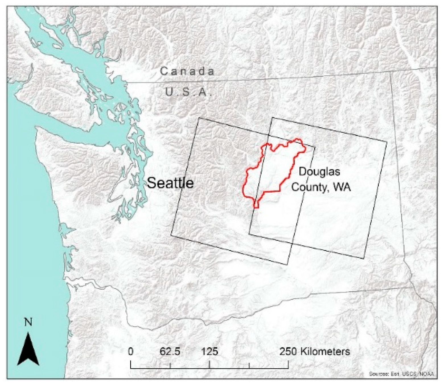
2.1. Study Area—Douglas County, WA, USA

We selected Douglas County, Washington in the northwest of the United States for our study area as it contained wetlands with variable hydrologic patterns of flooding and drying and has a high number of spectrally similar objects (Figure 1). Douglas County is part of the Columbia Plateau ecoregion, a semi-arid sage steppe ecosystem. Ranching and farming are the dominant land uses, and several urban areas are also present in the study area. Douglas County is bordered by the Columbia River with a low elevation of 180 m near the river and quickly rising to a high elevation of 1220 m before leveling off at the top of the plateau. The northern part of Douglas County was glaciated during the last ice age, approximately 20,000 years ago. Between 18,000 and 13,000 years ago, this area was impacted by a series of massive floods, which scoured the region. These geologic events created a topographically complex area with perched aquifers and intricate surface and subsurface flows, and a high density of isolated, depressional wetlands.

Wetlands in Douglas County fall on a continuum from seasonally flooded wetlands, which tend to be small in size, to permanently flooded wetlands, which tend to be larger in size. While there is considerable variability in the hydrologic regime of wetlands in Douglas County, they all follow a similar seasonal flooding and drying pattern, filling up in the winter months and drawing down in the drier summer months. Spectrally similar objects that occur throughout the landscape include, but are not limited to, shadows from topography, tree canopy, human built structures, rock outcrops and small mining operations. These areas mimic the spectral signature of surface water flooding.

2.2. Materials

2.2.1. Inputs

We downloaded 285 Landsat Thematic Mapper 4 and 5 satellite images from two Landsat scenes (Path 45, Row 27 and Path 45, Row 26) acquired between 1984 and 2011 from the United States Geologic Survey (USGS) GLOVIS website (http:/glovis.usgs.gov/) (

Table 1. Materials. TM = Thematic Mapper.

Datasets	Data Type	Source
Landsat TM 4 and 5	Raster	United States Geological Survey
Roads	Vector	WA Department of Transportation (http://www.wsdot.wa.gov/mapsdata/geodatacatalog/)
Slope Index	Raster	Derived from USGS 30 m digital elevation model
Irrigated Crops	Raster	WA State Department of Agriculture (https://agr.wa.gov/pestfert/natresources/aglanduse.asp)
Wetland Classification	Vector	Derived from OBIA of 1 m resolution aerial imagery (2006, 2011) (Halabisky et al. 2011, Halabisky et al. 2016)

). We only downloaded images acquired between March and October, as wetlands in the winter months are typically frozen or snow covered. We masked out all clouds and cloud shadows from the Landsat satellite imagery using the cloud mask provided by the USGS (https://landsat.usgs.gov/espa). We also used three additional ancillary datasets; a vector dataset of road lines from the Washington State Department of Transportation, a slope index calculated from a 10 m USGS digital elevation model, and a raster dataset of irrigated crop locations from the Washington State Department of Agriculture (Table 1). We buffered road lines by 30 m to capture the width of the road.

2.2.2. Training and Validation Data

We used a pre-existing wetland classification dataset for Douglas County to train and validate our RF model. The wetland classification was created through OBIA of a combined stack of 2006 and 2011 aerial images with 1 m pixel resolution, freely available through the United States Department of Agriculture, National Agriculture Imagery Program (NAIP). The classification was created through a user defined rule-based algorithm using wetland features, such as color, shape, and texture, determined from manual photo interpretation and is described in Halabisky, Moskal and Hall (2011) and Halabisky et al. (2016) [12,16]. Overall accuracy of the wetland classification was 90.3%.

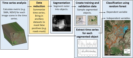
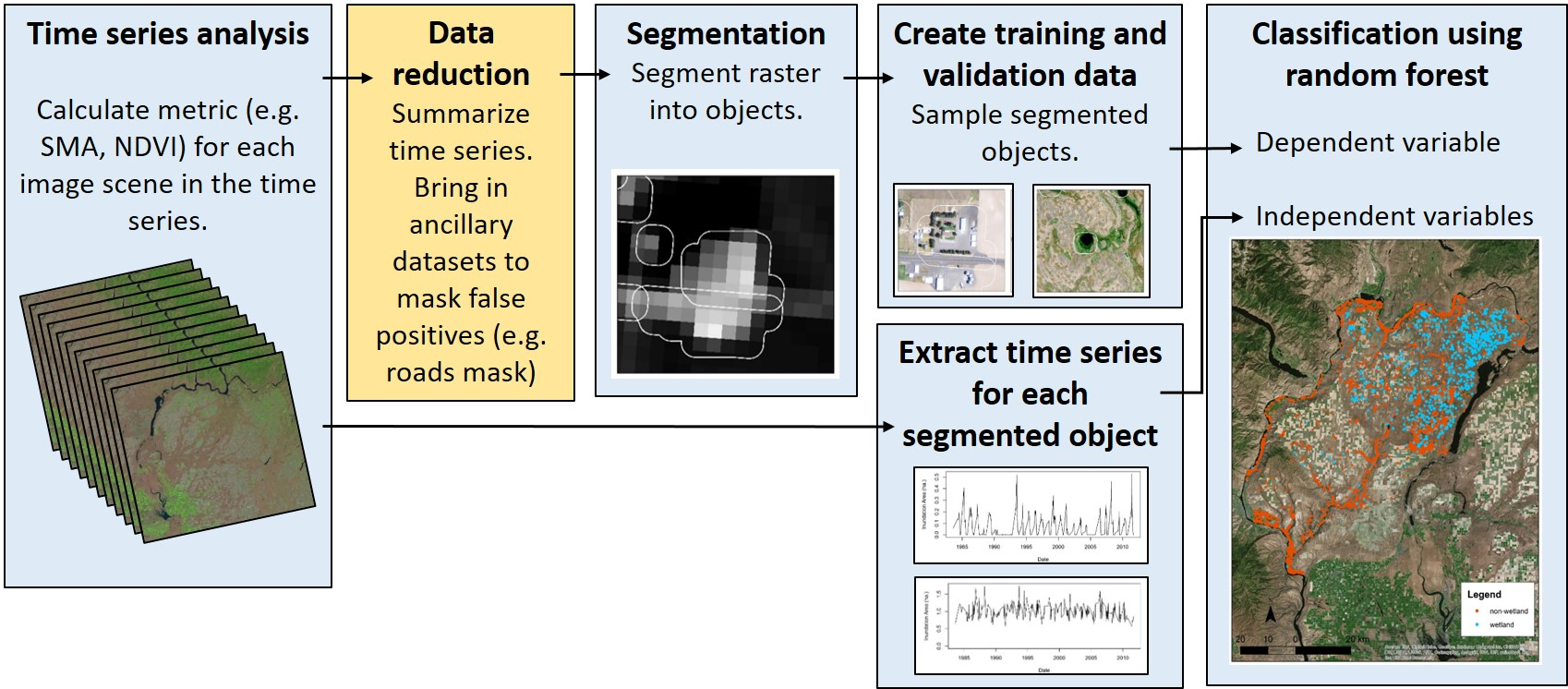
2.3. Developing Percent Surface Water Images

As a first step in our process, we converted the time series of Landsat imagery into sub-pixel estimates of surface water area using a constrained four-endmember spectral mixture analysis (SMA) model as outlined in Halabisky et al. (2016) [29] (Figure 2). Briefly, SMA uses the spectral signature of materials (called endmembers) found within the image scene to estimate the proportion of materials within the spectrum of a mixed Landsat pixel [36,37]. Two endmembers (water, sagebrush) were taken directly from each scene, while two endmembers (salt flat, wetland vegetation) were derived from six Landsat scenes as spectrally “pure” pixels are not available for every image. This technique provided a fractional estimate of surface water for each pixel, ranging from 0 to 1, for each image in the Landsat time series. Our previous research showed high correlation (R² = 0.99) between modelled surface water area estimates using SMA and actual surface water area [29].

2.4. Delineating Wetlands Using OBIA

We used OBIA to identify and delineate wetland objects using the time series of sub-pixel surface water area estimates. OBIA was performed using eCognition Developer 9.0 (Trimble, Westminster, CO, USA) using the SMA outputs derived from the time series of Landsat imagery. Segmentation is a first step in OBIA to convert raster images into vector objects. Segmentation using all bands from each image scene would be computationally intensive. Therefore, we reduced our time series from 285 Landsat scenes down to three raster images. Because wetlands in our study area typically flood in the spring, but may dry up in the summer, we calculated the spring (1 March–1 June) mean surface water percent cover for each pixel for three decades; the 1980s, the 1990s, and the 2000s. We chose to summarize it by decade rather than summarize across the entire time series to reduce errors of omission caused by wetland draining or agricultural influences that may have occurred during one of these decades.

As a first step, we ran a multiresolution segmentation on the three spring raster images and the slope index (scale parameter = 2), which created objects as small as 2–3 Landsat pixels (900 m²) in size. The scale parameter affects the size of the segmented objects and is related to the spatial resolution of the data inputs. We chose a scale parameter of two based on visual assessment of the segmentation output. Visual assessment is common when implementing a user defined rule-based approach in OBIA, as the impacts of every parameter and threshold decision cannot be easily quantified when run across the entire landscape [3]. Next, we used our ancillary datasets (Table 1) to mask out roads, steep areas (slope index > 5 degrees), and irrigated crops in order to limit the number of false positives. Smaller roads, driveways, and areas where road lines did not match could not be masked out. Because the slope index was derived from a 10 m digital elevation model, it was only useful at masking out large shadows created by steep topography and cliffs. While masking out slopes above five degrees cut down on the number of false positives, it also masked any potential slope wetlands. Therefore, slope wetlands, while rare in this landscape, are not included in this analysis.

Next, we classified objects that on average had 40% or greater estimates of surface water area from 1 April–1 June in the 1980s, the 1990s, or the 2000s as potential wetland objects. We chose this threshold through visual assessment with the goal of identifying all areas that held water in the spring, while limiting errors of commission. The SMA method detected low levels of surface water in highly disturbed areas, such as plowed fields. A threshold below 40% incorrectly mapped some upland areas as wetlands, increasing errors of commission. In addition, we wanted to limit analysis of wetland fluctuations to the primary basin and did not want to include areas that had overbank flooding, as this produced time series that overestimated the size of the wetland. Finally, we merged all neighboring objects together. We exported the results as a Geographic Information System (GIS) shapefile.

Following methods outlined in Halabisky et al. (2016), we buffered the output GIS shapefile by 30 m to address issues of imperfect alignment between satellite images. The buffered polygons were used to select (known as “extract by polygon” in ArcGIS) corresponding sub-pixel surface water area estimates from the Landsat time series, which were summed for each wetland using python tools in ArcGIS 10.1 (ESRI, Redland, CA, USA). This process created a unique time series of surface water area estimates spanning from 1984–2011 for each polygon. We realized that in using a low threshold (40% surface water inundation during the spring months) for classification, many of the polygons represented false positives. We explored the variability of temporal patterns between non-wetlands, small wetlands (<2 ha) and large wetlands (≥2 ha) by examining the variance and mean surface water area extent derived from the time series for all objects.

2.5. Identifying Wetlands Using the Temporal Pattern of Flooding and Drying

We used a RF classifier to identify wetlands based on their temporal pattern (Figure 2). RF is a nonparametric, bootstrapped, decision tree method [30]. We used the R package randomForest for our modeling [38]. The dependent (predicted) variables in our RF model were a classification of wetland or non-wetland objects. The independent variables were the surface water area estimates for each of the 285 images across time. The time series for the potential wetland objects we created was irregular because the two Landsat images scenes have different acquisition schedules. Additionally, many observations are missing due to areas that we masked out using the USGS cloud mask. RF does not allow for missing data. In order to resolve missing data, we fit a cubic spline to each potential wetland’s time series of Landsat data to fill in missing values using the R statistical package ‘spline’.

In order to construct a training and validation dataset of wetland and non-wetland objects for our RF model, we overlapped potential wetland polygons derived from the Landsat time series with our high-resolution wetland classification. Potential wetland polygons that overlapped with our high-resolution wetland classification were categorized as wetlands, while potential wetland polygons that did not overlap were categorized as non-wetlands. This resulted in a classification of 1015 wetland polygons and 2879 non-wetland polygons. Some wetlands were not present in the 2006 and 2011 aerial imagery, on which the high resolution classification was based, due to the ephemeral nature of wetlands or because of human caused disturbance. In order to achieve a near perfect reference classification dataset, we edited the merged wetland classification through manual photo interpretation of each classified object.

2.6. Exploring the Effects of Sampling Design on RF Classification Accuracy

We randomly selected half of the polygons in our reference classification to use as our validation dataset. While we were fortunate to have a large reference dataset for this area, we realize it is not common to have a large training wetland dataset. Therefore, we resampled 400 polygons from the remaining reference dataset to create a training dataset for our RF model. We selected our training data in three ways; (1) simple random sampling, (2) stratified random sampling by polygon size into large (≥2 ha) and small (<2 ha) objects, and (3) purposive sampling. The randomly sampled dataset contained 100 wetlands and 300 non-wetlands. The size-stratified random sample had 200 small polygons and 200 large polygons, which resulted in a sample of 143 wetlands and 257 non-wetlands. The purposive sampling was derived from manually selecting wetlands through visual assessment of the polygons using 1 m aerial imagery. The purposive sampling had 100 wetlands and 300 non-wetlands and was meant to mimic the practice of selecting training data by hand or in the field by selecting wetlands that could easily be detected in aerial imagery.

We trained the RF classifier using each of the three sample training datasets. For each RF model, we examined receiver operating characteristic (ROC) curves and calculated the area under the curve (AUC) [39]. The AUC is useful for assessing the accuracy of a classifier when datasets are unbalanced. We also performed a traditional accuracy assessment on the validation set [40]. Finally, we applied each of the RF model classifiers to the full potential wetland dataset, resulting in three classifications of wetland and non-wetland objects.

2.7. Monte Carlo Random Forest Modeling Using Time Series Data

In order to understand how the number of satellite image observations improved the classification accuracy of our model, we iteratively ran our RF model 200 times, increasing the number of observations used in the model. For this modeling approach we used the randomly sampled training dataset. We did this iterative process in three ways: (1) we added each observation into the RF model starting from the beginning of the time series, adding each image observation in sequential order; (2) we added observations in a random order, and; (3) we added observations that captured the variability in surface water area changes of wetlands across wet, dry, and average years of precipitation. We selected 18 observations from two wet years, two dry years, and two average years of precipitation. For each year, we included three observations that captured surface water area in late spring (April–May), early summer (June–July), and late summer (August–September) and added them into the RF model in the following pattern; wet year, dry year, average year. We plotted ROC, overall accuracy, errors of omission for the wetland class, and errors of commission for the wetland class for each iteration of the three RF models.

3. Results

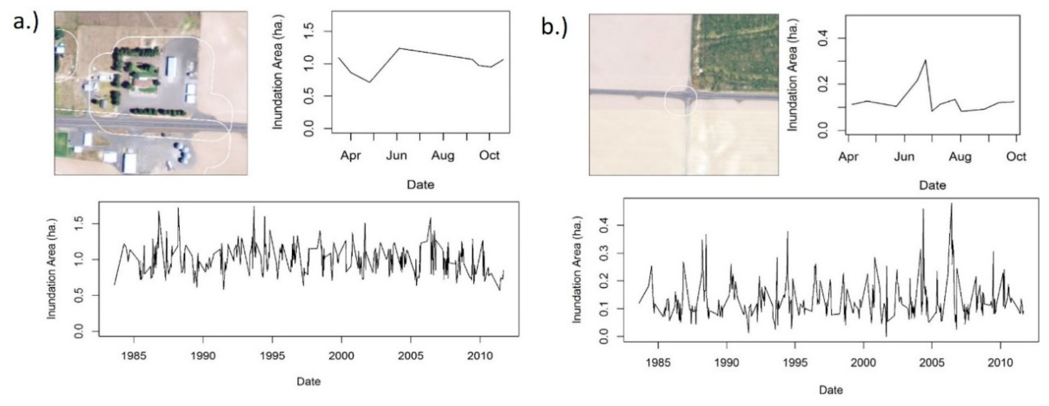
Our method using OBIA of sub-pixel surface water estimates identified 3894 polygons as potential wetlands. Only 1105 of these polygons were wetland objects. The remaining 2879 were spectrally similar false positives. Through visual assessment of the polygons using 1 m resolution aerial imagery, we determined that many of these false positives are spectrally similar to wetland inundation. These objects contain materials that absorb light, such as dark pavement, buildings, dark geologic features, and shadows (Figure 3). We also initially classified objects as potential wetlands that contained surface water, but are not considered wetlands, such as irrigated agricultural fields, canals, sections of streams, and rivers (Figure 3). These areas were not masked out using any of our ancillary data products.

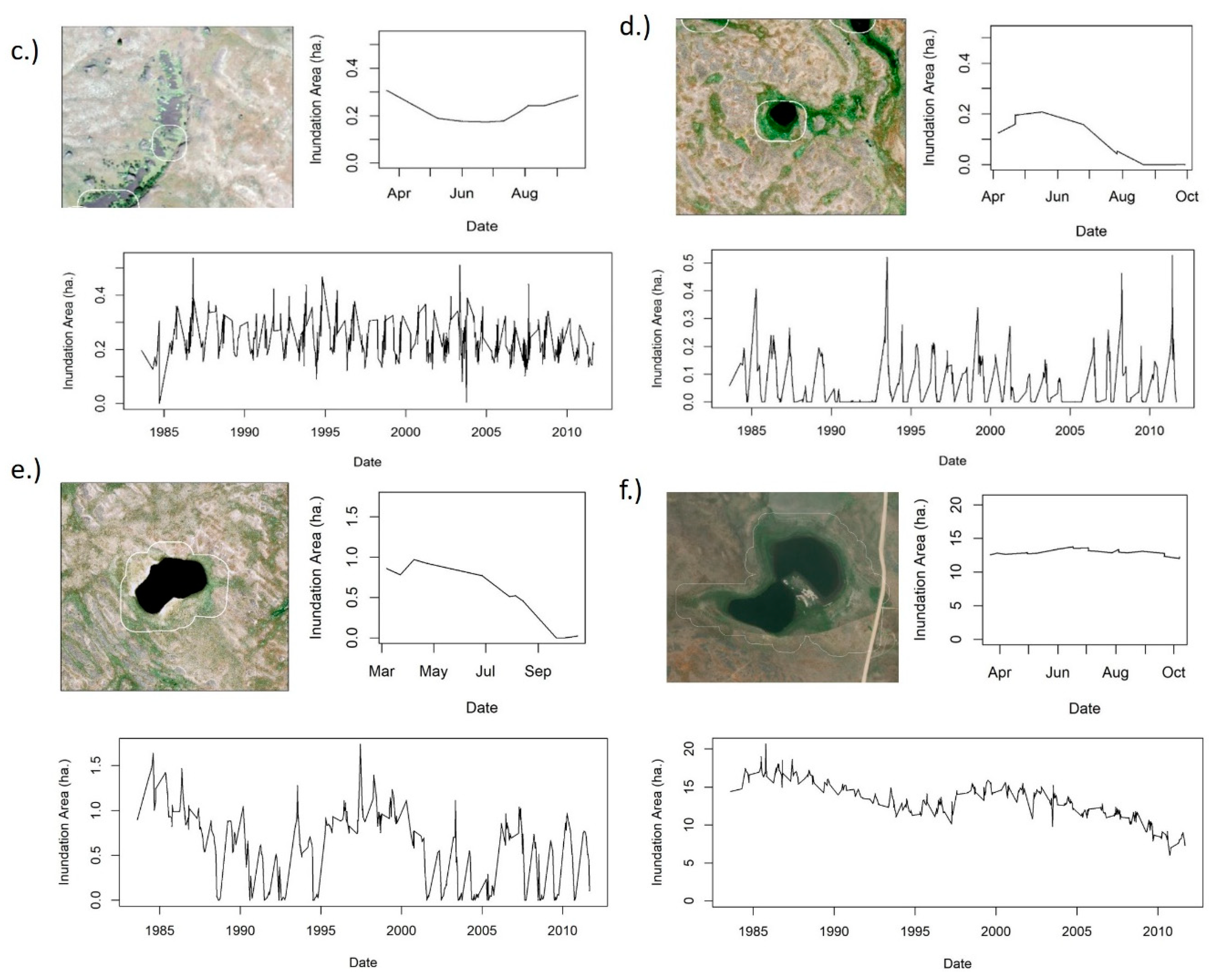
There was a lot of variability in temporal patterns between potential wetland objects (Figure 4). For wetlands, the changes in surface water area calculated through SMA represented seasonal and long-term changes in surface water inundation (Figure 5). Spectrally similar non-wetland objects did not have a similar seasonal or long-term temporal pattern (Figure 5). The distribution of the mean surface water area extent of non-wetlands had more overlap with large wetlands (≥2 ha) than small wetlands (<2 ha) (Figure 4). However, the opposite was true for the distribution of mean variance for non-wetlands. The distribution of variance for non-wetlands was more similar to small wetlands. Small wetlands (<2 ha) generally had a lower mean surface water extent than large wetlands (≥2 ha) and a lower variance than large wetlands.

3.1. Effect of Sampling Design for the Collection of Training Data

The sampling design for selecting training data for our RF model did not have a statistically significant impact on the overall accuracy of our modeled classification. There was no statistical difference in AUC between the random sample (95% CI: 0.927–0.953) or the random sample stratified by size (95% CI: 0.924–0.950), while the AUC for the purposive sampling was slightly lower (95% CI: 0.907–0.935) (Figure 6).

The overall classification accuracy was 91.52%, 92.09%, and 86.02% for the random sample, stratified sample, and purposive, respectively (

Table 2. Accuracy assessment for wetland classification using random sampling.

Reference Data
Classification Data	Wetland	Non-Wetland	Total	User’s Accuracy
Wetland	413	76	489	84.46%
Non-wetland	89	1368	1457	93.89%
Total	502	1444
Producer’s Accuracy	82.27%	94.74%
Overall Accuracy	91.52%

,

Table 3. Accuracy assessment for wetland classification using stratified sampling by size (<2 ha, ≥2 ha).

Reference Data
Classification Data	Wetland	Non-Wetland	Total	User’s Accuracy
Wetland	434	68	520	83.46%
Non-wetland	86	1358	1426	95.23%
Total	502	1444
Producer’s Accuracy	86.45%	94.04%
Overall Accuracy	92.09%

and

Table 4. Accuracy assessment for wetland classification using purposive sampling.

Reference Data
Classification Data	Wetland	Non-Wetland	Total	User’s Accuracy
Wetland	282	52	334	84.43%
Non-wetland	220	1392	1612	86.35%
Total	502	1444
Producer’s Accuracy	56.18%	96.40%
Overall Accuracy	86.02%

). The errors of omission and commission for the wetland class were similar for the random sample (17.73%, 15.54%) and the stratified sample (16.54%, 13.55%). For the purposive sample classification, the wetland classification errors of omission were 43.82% and errors of commission were 15.57%.

Visually, the mapped results did not vary substantially between the three sampling techniques. Classification error was evenly distributed throughout the county and did not have a strong spatial pattern. Non-wetlands tend to be in areas with increased shadows (plateau cliffs), irrigated areas, and along roads. Wetlands are clustered in the northern part of the county. The output classification using the random sample captured the variability of wetland types across Douglas County, but did miss some large wetlands (Figure 7). The overall accuracy was higher for small objects (92.79%) than large objects (87.6%). The stratified sample had a more balanced overall accuracy between small objects (92.13%) and large objects (89.64%) and the purposive sample had the largest disparity in overall accuracy between small objects (87.61%) and large objects (80.2%).

3.2. Effect of the Number and Arrangement of Available Images on Classification Accuracy

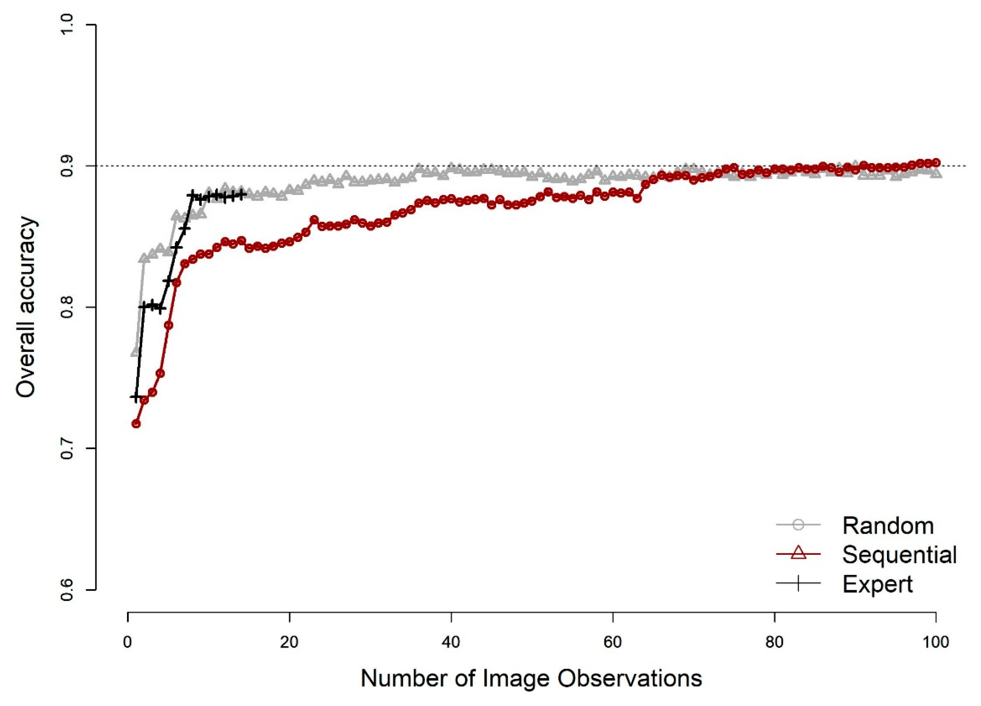
The AUC, overall accuracy, error of omission for wetlands, and error of commission for wetlands all improved when the number of image observations used as predictor variables in the RF model increased. However, increasing the number of image observations used in the RF model did not greatly improve classification accuracy beyond a certain number of image observations. This point of “leveling off” differed depending on how the images were added into the model: sequentially, randomly, or using expert knowledge (Figure 8). For randomly selected observations, there was little improvement in skill past the 25 observations included, and there was essentially no improvement from either random or sequential methods past about 65 observations included in the RF model.

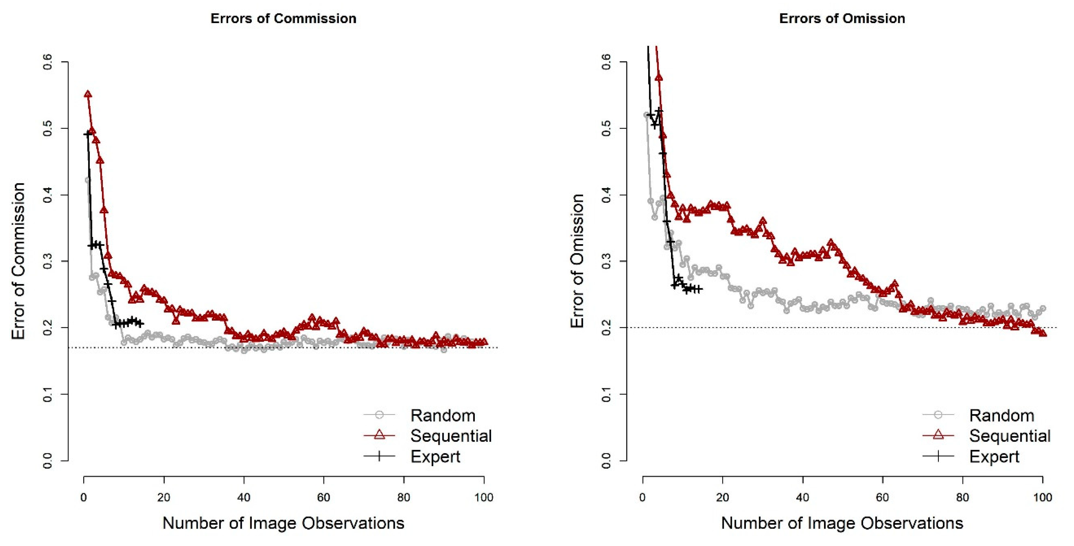
Overall accuracy achieved from images added through expert knowledge (87.98%) came close to reaching overall accuracy using a longer time series, although overall accuracy of 87.92% was reached after only eight image observations were added. These images represented spring, summer, and fall images from a wet year and dry year, and spring and summer images from an average year of precipitation. Note, however, that a random sample achieved essentially the same level of performance as the expert knowledge approach when about 10 image observations were used as the training data set. Expert knowledge selection methods were not clearly better than random selection in improving skill. Similar relationships were found between the number of image observations used and errors of omission and commission (Figure 9).

4. Discussion

Our approach exploiting the temporal domain classified wetlands with a high level of accuracy and reduced the number of spectrally similar false positives. Our initial classification relying only on the spectral information derived from the summarized Landsat imagery classified 2879 of the 3894 objects as potential wetlands (73.93%). These objects were spectrally similar to flooded wetlands. The addition of the temporal dimension reduced the number of false positives in the potential wetland classification, regardless of the sampling design selected or the number of image observations used.

Our comparison of the three sampling methods (random, stratified, purposive) used to select training data for our RF model did not produce large differences in overall classification accuracy or AUC. However, differences in wetland classification errors of omission were much larger between sampling methods (random 23.7%, stratified 15.0%, purposive 44.7%). This may be due to the fact that wetlands only represented 33.7% of the total potential wetland objects. While the randomly selected training data had a high overall accuracy, it did have noticeable errors of omission, particularly a few large permanently flooded wetlands being mapped as non-wetlands. These kinds of errors may be driven by the indiscriminate selection associated with random sampling. Because small wetlands are more numerous in our study area, there was a greater likelihood of randomly selecting small wetlands than larger wetlands. Therefore, the RF model trained on a random sample may not have captured the full variability of larger wetlands, causing them to be omitted from the classification. While stratifying the sample by large and small wetlands did not affect overall accuracy, it did correct some of these effects and correctly mapped more of these large wetlands. A stratified sample would be a better choice if it would be worse to omit a large wetland than a small wetland from classification.

In many cases, it is hard to get reliable wetland data for training and validation of OBIA classifications. Our purposive sampling strategy represents the practice of relying on pre-existing datasets (e.g., the US National Wetland Inventory) or selecting training data through photo interpretation where budget and time constraints may not allow for the collection of new randomly sampled training data. Often existing wetland datasets are biased towards larger, more intact wetlands that are easier to identify in aerial imagery or on the ground. While the results from our purposive sampling had relatively high errors of omission, it still had a high overall accuracy. If a purposive dataset is used, it is important to remember that existing bias in the training dataset will transfer to the resulting classification. For example, if training data derived from a pre-existing dataset omits wetlands that are hard to detect in aerial photos or in certain landscapes, this bias may be reflected in the errors of omission from the RF model classification results. In some cases using purposive sampling may be an acceptable practice if the goal of using an automated classification process is not to create an unbiased classification, but rather to reduce overall effort and cost of post-processing through manual clean up [24].

Our results demonstrate that the entire time series of Landsat satellite imagery is not required to identify wetlands from spectrally similar landscape features. However, temporal richness can improve the accuracy of a classification up until a point where accuracy improvement levels off. A random selection of image observations spanning the entire time series captured temporal variability of wetland objects as well as image observations selected through expert knowledge. Therefore, this approach may work in areas with sparse data or frequent cloud cover, regardless of whether imagery is available during wet, dry, or average precipitation years. A random selection of image observations is a straightforward way to characterize wetlands and had higher overall accuracy and lower errors of omission and commission than when observations were selected through expert knowledge (as is common practice) [9,41]. Our analysis also confirms, however, that the practice of selecting image observations from wet, dry, and average year precipitation can capture most of the variability unique to wetlands.

The large body of research leveraging remotely sensed time series data in pixel-based classification has already demonstrated how time series can improve the classification of features [15]. We believe that time series datasets can also improve OBIA classification as demonstrated here. Our generalized methods (Figure 2) can be reproduced in other settings using readily available data and software and does not require complicated modeling of the time series patterns themselves. Here, we focused on semi-arid wetlands, but inclusion of the temporal dimension could also improve classification of other landscape features such as meadows, agricultural crops, and other features that may be spectrally similar to the surrounding landscape. Further testing is required to confirm this hypothesis.

Here we created a simple classification of wetlands and non-wetlands. A further step would be to characterize each wetland by its hydrologic regime (e.g., seasonally flooded, semi-permanently flooded or permanently flooded). This can also be derived from the time series of inundated area either through use of the entire time series [29] or alternatively by analyzing sets of image observations [9].

Some of the steps we used were taken to reduce the dataset and improve computational processing time. The necessity and approach for data reduction will depend on the landscape, the size of the study area, the desired minimum mapping unit, and the processing power available. We were interested in mapping all wetlands, including small, ephemeral wetlands; therefore, we chose a low threshold (40% surface water inundation during the spring) for our initial classification of potential wetlands. Because of our low threshold, we initially mapped a relatively large number of false positives. These objects might not have been mapped if we had used a higher threshold value. We did not explore how changing the threshold value could impact final classification results. Future work to optimize this threshold might be productive in reducing the number of false positives selected at the outset, with resultant improvements in computational efficiency in carrying out subsequent steps.

A key strength to OBIA methods compared to pixel-based approaches is the ease in which data of varying resolutions can be combined so that the object can be characterized by the spatial, spectral, and temporal patterns associated with that object. Once an object is delineated, the data can be summarized at the object level, despite the varying differences in resolution. In this study we did not combine datasets together, focusing solely on the temporal resolution of wetland objects. Additional data optimized for other resolution domains could further characterize landscape features. For example, in order to get more precise wetland delineations, higher spatial resolution imagery could be included, hyperspectral imagery could be used to characterize wetland by species type, and lidar or radar could be added to characterize a wetland by additional hydrologic processes.

5. Conclusions

Our method using time series observations as input variables into a RF model improved distinction between wetland and upland objects by exploiting their temporal pattern. After more than 40 years of observing the Earth from remote sensing platforms, we now have a sizeable archive of temporal data cataloging ecosystem change ranging from decadal to daily time steps [42]. In the last decade, this archive has become increasingly accessible [43]. Most notably, the entire Landsat satellite archive is now freely available. Tools such as Google Earth Engine and the USGS batch download tool provide easy access to time series archives [44]. Parallel processing and cloud computing allows for rapid analysis of time series data. While time series analysis has been part of remote sensing for many decades, with improved computer processing and increased availability of time series datasets, it is now much easier to incorporate temporal characteristics into OBIA.