Article

Extracting Building Boundaries from High Resolution Optical Images and LiDAR Data by Integrating the Convolutional Neural Network and the Active Contour Model

1
Department of Geography and Planning, Sun Yat-Sen University, Guangzhou 510275, China
2
Guangdong Key Laboratory for Urbanization and Geo-simulation, Guangzhou 510275, China
3
School of Geographical Sciences, Guangzhou University, Guangzhou 510006, China
4
Guangzhou Urban Planning and Design Survey Research Institute, Guangzhou 510060, China
*
Authors to whom correspondence should be addressed.
Remote Sens. 2018, 10(9), 1459; https://doi.org/10.3390/rs10091459
Submission received: 18 July 2018 / Revised: 30 August 2018 / Accepted: 11 September 2018 / Published: 12 September 2018
(This article belongs to the Special Issue Remote Sensing based Building Extraction)

Abstract

:
Identifying and extracting building boundaries from remote sensing data has been one of the hot topics in photogrammetry for decades. The active contour model (ACM) is a robust segmentation method that has been widely used in building boundary extraction, but which often results in biased building boundary extraction due to tree and background mixtures. Although the classification methods can improve this efficiently by separating buildings from other objects, there are often ineluctable salt and pepper artifacts. In this paper, we combine the robust classification convolutional neural networks (CNN) and ACM to overcome the current limitations in algorithms for building boundary extraction. We conduct two types of experiments: the first integrates ACM into the CNN construction progress, whereas the second starts building footprint detection with a CNN and then uses ACM for post processing. Three level assessments conducted demonstrate that the proposed methods could efficiently extract building boundaries in five test scenes from two datasets. The achieved mean accuracies in terms of the F1 score for the first type (and the second type) of the experiment are 96.43 ± 3.34% (95.68 ± 3.22%), 88.60 ± 3.99% (89.06 ± 3.96%), and 91.62 ±1.61% (91.47 ± 2.58%) at the scene, object, and pixel levels, respectively. The combined CNN and ACM solutions were shown to be effective at extracting building boundaries from high-resolution optical images and LiDAR data.

Graphical Abstract

1. Introduction

Information regarding the spatiotemporal variation of buildings is important for various applications, such as geodatabase updating, environment management, and urban planning and development. Accompanying the revolutionary development of aerial and space remote sensing technology, identifying and extracting building boundaries from remote sensing data, such as high resolution optical images and recently airborne light detection and ranging (LiDAR) data, is a research frontier in the field of photogrammetry and remote sensing [1,2,3,4].
Among the tremendous efforts that have been made to extract building boundaries from remote sensing data [5], the active contour model (ACM) is a widely used method [6,7]. ACM, also referred to as the snake model, is a closed curve extracting method based on the idea of minimizing energy guided by external constraint forces such as lines or edges. ACM could generate smooth and closed object contours with various shapes [8]. Most existing ACMs could be categorized into edge-based and region-based ACMs. In the edge-based models, the contour is guided by the edge information [6]. The edge-based models are sensitive to the initial contour, as they focus on the image pixels, and the ACM contour often docks at the pseudo edges generated by textures [9]. Kabolizade, Ebadi and Ahmadi [10] used an improved snake model for building extraction. Compared with traditional ones, the snake model in their work performed efficiently, as they added a new height similarity energy and regional similarity energy, as well as gradient vector flow. However, their work depends on the initial contour selected. To solve this, Liasis and Stavrou [11] used Hue, Saturation and Value color space as well as the Red, Green, and Blue representation to extract the building boundaries from satellite images by using an ACM. A new energy term is encoded in this work for curve initialization, which leads to higher extraction accuracy. Another solution for curve initialization is to use region-based models which attract the contour by a region descriptor from the global or region context. Chan and Vese [12] presented a region-based active contour model that used a piecewise smooth function. The region-based models are not sensitive to the initial contour, although they are inefficient for the images in which the objects have inhomogeneity textures (i.e., intensity inhomogeneity). Li et al. [13] developed robust a region-scalable fitting (RSF) model that is capable of dealing with intensity inhomogeneity. However, one major limitation of the above-mentioned ACM methods is that confusion caused by trees and ground surfaces could result in errors on identified buildings. To avoid the influence of irrelevant confusing objects, Yan et al. [14] introduced a building model construction framework based on the snake model. They first derived non-terrain objects from LiDAR data and separated buildings from trees, and then extracted and refined the buildings by the snake model. In their work, they made use of a novel graph reduction method to extend the dynamic programming to 2-D planar topology snake model. Bypina and Rajan [15] used the object-based method to extract buildings from very high resolution satellite images, where scene objects are segmented by the Chan-Vese model, and tree objects are removed based on normalized difference vegetation index (NDVI). In practice, separating the buildings from other ground objects such as trees is often difficult by using only a vegetation index.
An effective building footprints detection method could provide helpful information to avoid the effects of other terrain objects, and improve the extraction of building boundaries accordingly. Methods such as the classic hierarchical stripping classification and machine-learning-based classification have been developed to detect building footprints [16,17,18]. In the classic hierarchical stripping approach, building footprints are separated from vegetation footprints, other off-terrain footprints, and terrain footprints progressively [19]. Awrangjeb and Fraser [20] proposed a method for automatic segmentation of LiDAR data. The ground and the non-ground footprints are separated based on a “building mask”. The building roof footprints are then segmented from the non-ground cluster of points and refined by rules. In the method of Wang et al. [21], the building boundaries are detected by a four-step method. The thresholding method is applied to separate footprints with high heights from others. Oriented boundaries are detected by an edge-detection algorithm. Building and non-building objects are classified by two shape measures finally. When extracting building footprints, the hierarchical stripping classification is operationally complicated due to multiple-step operation and manual interaction.
In the past few decades, researches have used the machine learning approaches, such as Artificial Neural Networks (ANN) [22,23], Support Vector Machine (SVM) [24,25], AdaBoost [26] and Random Forests (RF) [27], to extract building footprints. The machine learning approaches could establish a model that detects building footprints by learning the classification rules automatically using training data [28]. Lodha et al. [29,30] employed SVM and AdaBoost classifiers for LiDAR data classification. Du et al. [31] presents a semantic building classification method by using RF classifier from a large number of imbalanced samples. The RF classifiers are improved in two aspects: one is the voting distribution ranked rule for imbalanced samples, and the other is the feature importance measurement. Structured prediction methods, such as Conditional Random Field (CRF), are also used. Niemeyer et al. [32] integrated a RF classifier into a CRF framework, in which the CRF probabilities for the classes are computed using a unary potential and a pairwise potential. The RF approach is more reliable when compared to the linear models for the CRF computation. Overall, the performances of the traditional methods are often dependent on the derived handcraft features. Recently, deep learning has shown a great ability in high level feature extraction or object detection. Vakalopoulou et al. [33] proposed a convolutional neural network (CNN) for deep feature learning. The deep features and additional spectral information were then fed to a SVM classifier for automated building detection, and the result was refined by Markov Random Field. However, they only used CNN for deep features extraction; accordingly, the procedure of feature extraction cannot optimize the classification adaptively. Erhan et al. [34] developed a saliency-inspired neural network for object detection. The network contains several convolutional layers, pooling layers, and full connected layers. Although the abstract features derived from the convolutional layers are helpful to classify the categories of objects in an image, the pooling layers in the architecture reduces the image resolution. Accordingly, the details of the object are lost, and the specific outline of the object cannot be detected well. In essence, classic CNN is more suitable for patch-based image category classification rather than pixel-wise classification. Fully convolutional networks (FCNs) add upsampling layers and convert the full connected layer into the convolutional layers, which could up-sample the feature maps to the original size. Li et al. [35] compared the performance between the fully convolutional network [36] model and shallow models in building detection. A qualitative and quantitative analysis showed that FCN gives better results than shallow models. Although FCN improves the pixel-wise classification, the results are not sensitive enough to the details, and the shapes of the building boundaries are still blurred. Compared with FCN, the symmetrical encoder-decoder network SegNet [37] improves the boundary delineation, and is easy to incorporate into any end-to-end architecture, such as FCN. Although CNN shows robust ability in object classification, it suffers from the “salt and pepper” artifacts inevitably, which in turn affects the detected object boundary.
Recent work has also explored CNN for contour extraction. Maninis et al. [38] proposed an architecture called convolutional oriented boundaries for multiscale oriented contours producing. However, the model is designed for natural images. Remote sensing images are often complex scenes, which are not guaranteed to work. Rupprecht et al. [39] developed a deep active contour model. In their work, they predicted the vector point of the contour by a CNN. Nevertheless, they also need an initial curve for image patch deriving, which is costly and time-consuming.
To reduce the influence of other ground objects and “salt and pepper” artifacts, we developed an automatic building boundary extraction method from high-resolution optical images and LiDAR data by integrating CNN and ACM together. We conducted two types of experiments: the first was to extract the building boundaries directly by integrating ACM into CNN construction progress; the second was to use CNN for initial building footprint detection, and apply ACM for the post process.

2. Materials and Methods

2.1. Study Materials

Two different datasets are used in our experiment. The first (hereinafter referred to as the Potsdam dataset) is the ISPRS benchmark data of Potsdam that covers a historical city with large buildings. The dataset contains 38 patches, and each provides high-resolution orthorectified aerial photograph and digital surface models (DSM) with pixel size 6000 × 6000 at the spatial resolution of 5 cm. The aerial photograph has 4 channels: red, green, blue, and near-infrared bands. NDSM is derived based on automatic filtering. The dataset was classified into six land cover classes, of which five classes were merged into non-buildings. Among the 38 patches, 24 patches were labeled by the benchmark test organizers and were used for the training of the CNN, whereas 3 patches (Potsdam 2_13, Potsdam 6_15 and Potsdam 7_13) were used for validation (Figure 1). The ground truths of the three patches are obtained by manual labelling.
The second dataset (hereinafter referred to as the Marion dataset) that covered Marion in Indiana, USA was downloaded from the Indiana Spatial Data Portal (ISDP). The dataset (Figure 2) includes orthophotography (RGBI) and LiDAR/elevation data. The ground sampling distance of the optical image is about 0.15 m, and the LiDAR data is about 1 point/m2. We choose seven blocks for CNN training from the Marion County with the size of 10,000 × 10,000 each. We label the images as buildings and non-buildings using the vector data of Open Street Map, as well as by manual labeling. NDSM is derived from the original LiDAR data. The CNN networks are trained by the composite images of RGB+IR+NDSM. The validation data in the Potsdam and Marion datasets have a window size of 2000 × 2000 pixels and 1200 × 1800 pixels, respectively.

2.2. Preliminaries

CNN: the encoder-decoder architecture, such as SegNet that is capable of performing semantic pixel labeling of an image, is employed for building footprints detection. For the task of building footprint detection, we can predict the probability that each pixel belongs to a building or non-building in the image by using SegNet. SegNet is a supervised approach with a convolutional-deconvolutional structure. It has a set of convolutional stages, and typically includes fine layers, including the convolutional layer, the activation function layer, the pooling layer, the batch normalization layer, and the up-sample layer. The convolutional layer is the core component in the convolutional stage, and applies a series of filters for feature extraction. The batch normalization layer aims to avoid the vanishing gradients or the explosive gradients. The activation function layer controls the activation level of a neuron for the forward signal transform. A rectified linear unit (ReLU) is often used for non-linear mapping of the input features. The pooling layer generalizes the input features by applying a non-overlapping window to achieve the down-sampled feature maps. The up-sample layer is to resample the feature maps which were down-sampled by the pooling layers to original image sizes. The feature maps are fed into the softmax for pixel-wise classification. A detailed description on SegNet may be found in [37]. The final classification map for a given image can be obtained by calculating the category corresponding to the maximum probability of each pixel.
Active contour model: the ACM method that accounts for both edge and region [40] is employed for the building boundary refinement. Given an image I ( x , y ) : Ω R , Ω R n is the image domain. Suppose a closed contour C Ω , which separates the image into two regions Ω 1 and Ω 2 , where Ω 1 and Ω 2 denote the exterior and interior of C, respectively. For a given pixel x Ω , the energy function of the ACM is defined as follows:
E ( C , f 1 ¯ , f 2 ¯ ) = μ C g ( | I [ C ( s ) ] | ) d s + i = 1 2 λ i Ω i K σ ( x y ) | I ( y ) f i ( x ) | 2 d y d x  
where, the first term is the edge energy. g ( x ) = 1 1 + ( x + K ) 2 is the edge function, and K is the contrast coefficient of the edge function g which is greater than 0. The second term is the RSF energy. The positive parameters μ and λ i are the weights of the two terms, respectively. f i ( x ) is the approximate image intensity inside or outside the contour C. I ( y ) is the intensity of a local region centered at pixel x, and σ is the size of the region. The bigger that σ is, the higher the calculation complexity of the model.
We employ the variational level set method for the above model solution. The closed contour C Ω is presented by the level set function ϕ Ω . An arbitrary rectangle is chosen for the initialization of contour C, and the value of level set function ϕ is as follows:
{ ϕ ( x , y ) > 0   o u t s i d e   t h e   c o n t o u r   C ϕ ( x , y ) = 0   o n   t h e   c o n t o u r   C   ϕ ( x , y ) < 0   i n s i d e   t h e   c o n t o u r   C  
Moreover, we introduced the regularization Heaviside function H ( ϕ ) , as well as its derivative δ ( ϕ ) , and added the level set regularization term to Equation (1).

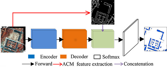
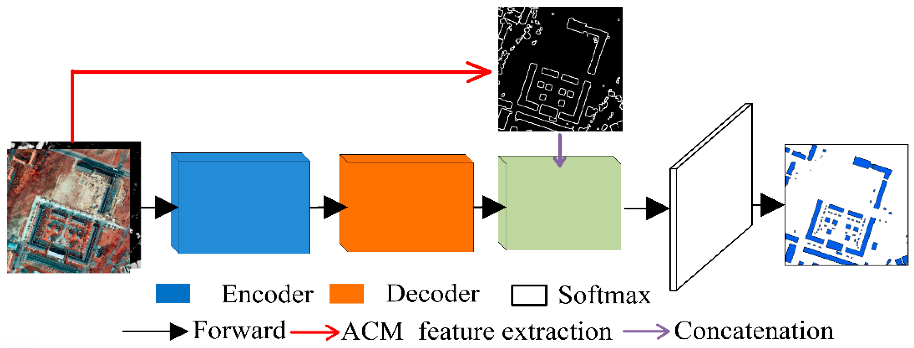
2.3. Building Boundary Extraction Based on CNN and ACM

We developed two strategies for CNN and ACM combination in this study. For the first (CNN_ACM_1), we integrated ACM into CNN construction progress, while the second solution (CNN_ACM_2) starts with CNN for building footprints detection, and then uses ACM for post processing. Figure 3 shows the frame work of the first solution. The optical images and NDSM are fed into the encoder-decoder architecture for deep feature learning. Meanwhile, ACM is used to extract the boundaries features to improve the boundaries perception. The ACM hand-crafted features and CNN deep features are concatenated before the softmax classifier for the final classification.
Figure 4 illustrates the framework of the second solution. CNN is first applied to detect the candidate building footprints, which are then clustered into subsets for individual building patch generation. Each building boundary is refined by ACM and mosaicked into a whole scene. Details on these processes as follows.
CNN could misclassify pixels, resulting in apparent salt and pepper artifacts; as such, ACM is used to refine the extracted building footprints. To reduce the dimensionality of the ACM searching space, we generate individual building patches from the CNN classification results for feeding into the ACM model. Figure 5 illustrates the detailed procedures to generate individual building patches. Given the remote sensing data, building footprints are first identified based on the mean shift clustering method (Figure 5b). The triangulated irregular network is then established for each individual building footprint using Delaunay triangulation, and the areas of the triangulated irregular network are delineated (Figure 5c). A buffered area (the buffer distance varies from 5–10 m depending on the building sizes in the scene) of the triangulated irregular network (marked with the black curve in Figure 5d) is built as some of the buildings that are not completely detected in CNN, and small footprints less than a priori minimum building area are then deleted. The minimum bounding rectangle (MBR) of the triangulated irregular network area is finally generated for the building patch cropping (Figure 5e, the red rectangle). In the ACM boundary extraction, the edges in the high resolution optical images are often located at the texture changes; however, they appear at the places where the elevation changes in NDSM. Comparatively, the contrast between building objects and ground surfaces is stronger in NDSM than in high resolution optical images, and thus, we employed NDSM for further ACM refinement (Figure 5f). After the boundary extraction, all building patches are mosaicked based on the cropping position to the original scenes.

2.4. Experiment Setup

Our CNN architecture is running on NVIDIA TITAN X based on Caffe, and the ACM algorithm and the RF classification algorithm are implemented by Matlab R2014a. The remote sensing images in this study are processed by ArcGIS 10.4.1 and ENVI 5.3. The building samples from the ISPRS benchmark dataset and Open street map (OSM) were used for training. High resolution optical images and NDSM are cropped into small patches of 300 × 300 pixels. For the Potsdam and Marion datasets, 8400 and 8092 patches are used for CNN model training, respectively. The trained CNN are then used for mapping building footprints.
To understand the algorithm robustness, the proposed methods are compared with the methods that use CNN [37] or ACM [40], as well as the state of the art classification method, RF [27]. The training and inference manners of RF and CNN are quite different. The stratified random sampling strategy is used for RF method, and the samples are only from the test images. For the ACM method, the entire scene was fed into the ACM model for building boundary extraction. The detected building footprints in the raster format were converted to the vector format. Small objects, i.e., less than the minimum building area, e.g. often cars, small trees, or the salt and pepper noise caused by classification, are removed. All the building boundary results are post-processed using the DP algorithm [41].

2.5. Assessment

Method assessments were conducted at the scene, object, and pixel levels. Detected buildings are split or merged based on the topological relations, as identified by the topological clarification method proposed by Rutzinger et al. [42]. The metrics of Completeness (Comp), Correctness (Corr), and F1-score (F1) were derived as follows:
C o m p = T P / ( T P + F N ) C o r r = T P / ( T P + F P ) F 1 = 2 × C o m p × C o r r C o m p + C o r r
where, TP, FP and FN have different definitions in the three levels, and they are described in more detail below.
At the scene level, we establish correspondences between buildings in the detected results and ground reference by their overlapping rate (Equations (4)). The overlapping rate is derived as follows:
R overlap = A overlap / A ref  
where, A overlap is the overlapping area of the detected building and the corresponding building in the ground reference and A ref is the area of the building in ground reference.
At the scene level, the detected results are categorized based on five different critical thresholds for the overlapping rates (i.e., Toverlap = 10%, 30%, 50%, 70%, and 90%). The detected buildings with the overlapping rates larger than the critical threshold are labeled as TP, the reference buildings with the overlapping rates lower than the critical threshold are considered as FN, and the detected buildings with the overlapping rates lower than the critical threshold are considered as FP.
At the object level, we only evaluated each detected building which has an overlap with ground reference data set (i.e., the TPs in scene level). The object level metrics give estimates of a single building. Object level TP denotes the overlapping area between the detected building and the reference building, FN denotes the undetected area of the reference building, and FP denotes the falsely detected area of the detected building. With the defined TP, FN, and FP, the metrics of Comp, Corr, and F1-score are first derived for each individual building, and then averaged for all the objects across the scene.
To perform assessments at the pixel level, both the detected results and the reference data are converted to the raster formats and then compared with each other. At the pixel level, the pixel correctly detected as building is referred as TP. FN denotes the building pixel that is not detected, and FP denotes the pixel that is not a building in the reference data, but which was misclassified as building.
The three-level assessment shows the performance of our method in different ways. The scene-based assessment is based on the overlapping area, indicating the accuracy of the whole scene. The object-based metrics can evaluate how a building object can be extracted. Pixel-based metrics are easily done by comparing the detect images and ground truth. However, pixel-based assessment may be distorted owing to the problems of building boundaries [42]. The different metrics are indicative to the algorithm accuracies from different aspects, but should not be compared across different levels.

3. Results

3.1. Building Boundary Extraction Results

Figure 6 shows visual comparisons among methods. ACM often misclassifies tall trees as buildings, and fails to extract buildings of low height due to background confusion. RF can better extract building footprints than ACM, but it frequently generates classification results with apparent “salt and pepper” artifacts. CNN outperforms both ACM and RF in distinguishing trees from buildings, whereas CNN could misclassify the buildings with heterogeneous textures. The methods of both CNN_ACM_1 and CNN_ACM_2 obtain reasonable results, as compared using the algorithms above.
As marked with red rectangles in Figure 6, buildings with inconsistent roof texture are rarely extracted correctly in CNN, whereas the use of ACM clearly refines the building boundaries. Figure 7 shows the details of the marked building in Potsdam 2_13. CNN_ACM_2 tracks the boundary fairly well, whereas CNN_ACM_1 can detect the building, but the detected boundary is not accurate enough. ACM underestimates the building and some building footprints are not detected. Both CNN and RF have the salt-and-pepper artifacts. For buildings with vegetation on top of the roof (marked with yellow rectangles in Figure 6), CNN_ACM_2 could provide good results, while CNN_ACM_1 and CNN failed to extract the roof areas covered by vegetation (see details in Figure 7, Potsdam 6_15). Results detected by RF still have the salt and pepper artifacts. The building missed by the other methods as marked by blue rectangles in Figure 6 could be detected well using CNN_ACM_1. For the tower with complex structure in Potsdam 7_13 (marked with green rectangle in Figure 6), CNN_ACM_1 yields a more complete result than other methods. The buildings in Marion dataset have simple structures and similar spectrum. All methods except ACM and RF successfully extracted the building boundaries.

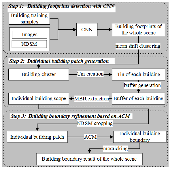
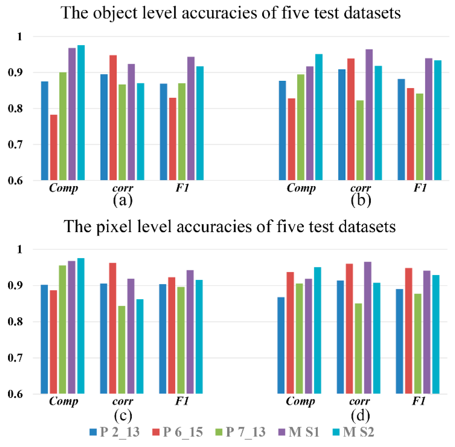
3.2. Performance Assessment

Figure 8 presents the assessment results of the proposed building boundary extraction methods for five test scenes at the scene level (see the details in Table A1 and Table A2). The overlapping thresholds are used to determine whether the detected building is a TP at the scene level. This means that if the overlapping rate R overlap of a building is lower than the threshold, it will be considered as an undetected one. Obviously, the methods could detect more TPs and achieve higher accuracies using low overlapping thresholds than high overlapping thresholds. For the Potsdam dataset, CNN_ACM_1 achieves the accuracies higher than 90.41% when the overlapping threshold is less than or equal to 30%. For 50–70%, the scene level accuracies are almost all above 82.05%, except Potsdam 6_15 at Toverlap = 70%. While for the highest threshold (90%), the average accuracy of the three scenes is 73.22%. When using CNN_ACM_2, similar accuracies were obtained, except for a slight drop in Potsdam 6_15. In the Marion dataset, the accuracies are higher than those of Potsdam, as few buildings are missed in both scenes. CNN_ACM_1 obtains the accuracies of above 98.00% for the overlapping threshold less than or equal to 70%. The accuracies are above 95.00% when assessed by the threshold of Toverlap = 90%. CNN_ACM_2 obtains higher accuracies in Marion S1 than CNN_ACM_1, and slightly lower accuracies in Marion S2.
Figure 9 shows the assessment of the extracted building boundaries at the pixel and object levels (see the details in Table A3 and Table A4). At the object level, the mean values of Comp, Corr, and F1 for all the detected buildings overlapped with ground truth are derived and shown in Figure 9a,b. Comp represents the similarity between overlapping area Aoverlap and ground truth, while Corr represents the similarity between overlapping area Aoverlap and detect results. F1 can be regarded as a weighted average of Comp and Corr. For the method of CNN_ACM_1, we can see that the detected buildings have good area similarity compared with ground reference objects: the mean F1 scores are above 82.98% for all the five test scenes, among which Marion S1 achieves 94.35%. For the methods of CNN_ACM_2, the mean F1 scores of all the assessed buildings are above 84.15%, and the highest accuracy (93.96%) is also obtained for Marion S1. The accuracies at the pixel level (Figure 9c,d) can be perceived as a kind of average of scene and object level assessment. The average F1 score of the five test scenes at the pixel level is 91.62% for CNN_ACM_1, and 91.72% for CNN_ACM_2.

3.3. Comparative Analysis

Figure 10 compares the assessment results of different building boundary extraction methods across two datasets. The horizontal axis denotes the assessment level, namely, the object level, the pixel level, and the scene level with five different overlapping thresholds. The vertical axis denotes the accuracies of F1 scores.
For the scene of Potsdam 2_13, CNN_ACM_1 performs the best in the five scene level assessments, and the method of CNN_ACM_2 comes second. This means that CNN_ACM_1 can detect more buildings which overlap with ground truths than other methods. At the object level, CNN_ACM_1 also works the best. Higher object-level accuracy implies that the detected buildings have better area similarity with ground truth. The other methods, CNN, ACM and RF, all work worse than our proposed method on all the three levels. In Potsdam 6_15, CNN_ACM_1 performs the best in all the five scene level assessments. This is because CNN_ACM_1 detects several small buildings which other methods do not extract. However, the detected building boundaries are poorer than CNN_ACM_2, as shown in Figure 6. At the object level and pixel level, CNN_ACM_2 undoubtedly achieves the best results. The accuracy of CNN_ACM_1 is slightly higher than that of CNN and RF, and ACM is the worst. In Potsdam 7_13, the opposite result is obtained. CNN_ACM_2 detects more buildings, but the building shapes are worse than with CNN_ACM_1. In Marion S1, CNN_ACM_2 and CNN performs best in the scene level assessments. CNN_ACM_1 and RF miss a small building, and their accuracies are a bit worse. ACM also obtains the worst accuracy. For Marion S2, the accuracy of RF is as good as CNN_ACM_1, except Toverlap = 90%. The other three methods show the same ability in the scene level. CNN_ACM_1 achieves the best object level accuracy, and RF obtains the highest pixel level accuracy, respectively. Overall, our proposed methods are effective for buildings under various scenes. CNN_ACM_1 obtains the best results at the scene level, and CNN_ACM_2 is good at the object level. CNN and RF only attain satisfactory results in simple building types.

4. Discussion

In practice, most building footprints can be detected by CNN, which shows a powerful ability in distinguishing buildings and vegetation. However, salt-and-pepper artifacts remain inside a building or on the building boundaries in the classification results. Accordingly, the completeness of a building needs to be improved to some extent. As reported in Section 3, the introduction of ACM improves the accuracies obviously when the footprints of a building are partly missed in CNN classification. On the whole, the integrated solution of CNN_ACM_1 works the best, except in the case of buildings with vegetation on the roof, as it can detect more building areas than other methods. CNN_ACM_2 also performs well on the building boundary refinement, which benefits from the excellent edge extraction capability of ACM, as the contour of ACM can stop at the relative reliable building edges. Moreover, the individual building patch generation process reduces the calculation range of ACM. The method of RF can obtain good results in simple scenarios. However, it has a more severe salt and pepper effect than CNN. The method of ACM is often influenced by other ground objects such as trees. In terms of the performance of the proposed methods in the two datasets, the results for the Marion dataset are better than Potsdam in almost all the three assessment levels. Buildings with diverse shapes and different spectral in Potsdam make it harder for accurate extraction, while the simple structures and spectral characteristics of buildings in Marion resulted in high accuracy.
Although the proposed models perform well, further improvements are needed. First, the generalization ability of the network should be improved. CNN_ACM_1 shows poor handling capacity in case of buildings with vegetation on the roof. This is mainly due to the different data distribution of the training data and the test scene, although they have the same data sources. The reason that RF can detect this kind of building is attributed to the sampling strategies: it selects samples from the very classification images. Second, a softer and more effective building boundary regularization method is required. The DP regularization algorithm reduces the building extraction results to some extent.

5. Conclusions

We developed a method for building boundary extraction using CNN and ACM. Two kinds of strategies are designed. The first employs ACM for boundary feature extraction, which is then fed to the CNN architecture. The second starts building footprints detection with CNN classification, and then clusters the footprints to obtain subsets of candidate buildings, from which the buffer of every building is constructed and the MBR is derived. Next, the NDSM of the scene are cropped by the MBRs. Finally, the cropped NDSMs are fed to the ACM for building boundary refinement, and mosaicked into a whole scene based on their original positions. The benefits of our method are as follows: (1) the proposed solution can reduce the influence of vegetation and salt and pepper artifacts. (2) It can extract buildings which are similar to the ground surfaces, which are missed in the other methods. When testing two datasets with various building shapes, we obtained better results than other three methods in the five test scenarios. In the future, we hope to extend our method to other complex building types, such as the archaeological buildings.

Author Contributions

Y.S. was responsible for the conceptualization and the methodology, and wrote the original draft; X.Z. (Xinchang Zhang) acquired the funding and supervised the study; X.Z. (Xiaoyang Zhao) contributed materials, performed the experiments of Section 3.1 and contributed to the figures; Q.X. reviewed and edited the draft, and contributed to the article’s organization.

Funding

This research was funded by the National Natural Science Foundation of China (grant Nos. 41801351 41431178, and 41875122), the Natural Science Foundation of Guangdong Province, China (grant No. 2016A030311016), the National Administration of Surveying, Mapping and Geoinformation of China (grant No. GZIT2016-A5-147), and the Key Projects for Young Teachers at Sun Yat-sen University (grant No. 17lgzd02).

Acknowledgments

The authors wish to thank the study material providers. The Potsdam data were produced by International Society for Photogrammetry and Remote Sensing: http://www2.isprs.org/commissions/comm3/wg4/2d-sem-label-potsdam.html. The Marion data were obtained from the Indiana Spatial Data Portal (ISDP): http://gis.iu.edu/datasetInfo/index.php. We also would like to thank the anonymous reviewers for their constructive comments.

Conflicts of Interest

The authors declare no conflict of interest.

Appendix A

Table A1. Accuracies of CNN_ACM_1 at the scene level.
ScenesMetricsOverlapping Threshold
10%30%50%70%90%
Potsdam 2_13Comp0.97010.95520.91040.83580.6716
Corr1.00001.00001.00001.00001.0000
F1 score0.98480.97710.95310.91060.8036
Potsdam 6_15Comp0.97300.89190.83780.70270.5405
Corr0.92310.91670.91180.89660.8696
F1 score0.94740.90410.87320.78790.6667
Potsdam 7_13Comp0.90480.90480.85710.76190.7143
Corr0.90480.90480.90000.88890.8824
F1 score0.90480.90480.87800.82050.7895
Marion S1Comp0.96970.96970.96970.96970.9091
Corr1.00001.00001.00001.00001.0000
F1 score0.98460.98460.98460.98460.9524
Marion S2Comp1.00001.00001.00001.00000.9600
Corr1.00001.00001.00001.00001.0000
F1 score1.00001.00001.00001.00000.9796
Table A2. Accuracies of CNN_ACM_2 at the scene level.
ScenesMetricsOverlapping Threshold
10%30%50%70%90%
Potsdam 2_13Comp0.94030.94030.89550.82090.6567
Corr0.98440.98440.98360.98210.9778
F1 score0.96180.96180.93750.89430.7857
Potsdam 6_15Comp0.89190.89190.83780.70270.5405
Corr0.82500.82500.81580.78790.7407
F1 score0.85710.85710.82670.74290.6250
Potsdam 7_13Comp0.95240.95240.85710.85710.7619
Corr0.90910.90910.90000.90000.8889
F1 score0.93020.93020.87800.87800.8205
Marion S1Comp1.00001.00001.00001.00000.7576
Corr1.00001.00001.00001.00001.0000
F1 score1.00001.00001.00001.00000.8621
Marion S2Comp1.00001.00001.00001.00000.8800
Corr0.96150.96150.96150.96150.9565
F1 score0.98040.98040.98040.98040.9167
Table A3. Accuracies of the proposed method at the object level.
ScenesCNN_ACM_1CNN_ACM_2
Mean_CompMean_CorrMean_F1Mean_CompMean_CorrMean_F1
Potsdam 2_130.87520.89490.86930.87690.90860.8822
Potsdam 6_150.78270.94810.82980.82780.93860.8567
Potsdam 7_130.90090.86690.87010.89480.82260.8415
Marion S10.96810.92350.94350.91700.96460.9396
Marion S20.97560.87040.91730.95140.91810.9333
Table A4. Accuracies of the proposed method at the pixel level.
Scenes CNN_ACM_1 CNN_ACM_2
CompCorrF1CompCorrF1
Potsdam 2_130.90210.90540.90380.86780.91400.8903
Potsdam 6_150.88660.96260.92300.93690.96010.9483
Potsdam 7_130.95550.84380.89620.90580.85090.8775
Marion S10.96790.91870.94270.91840.96540.9413
Marion S20.97550.86210.91530.95110.90780.9290

References

  1. Awrangjeb, M. Using point cloud data to identify, trace, and regularize the outlines of buildings. Int. J. Remote Sens. 2016, 37, 551–579. [Google Scholar] [CrossRef] [Green Version]
  2. Laefer, D.F.; Hinks, T.; Carr, H.; Truong-Hong, L. New advances in automated urban modelling from airborne laser scanning data. Recent Pat. Eng. 2011, 5, 196–208. [Google Scholar] [CrossRef]
  3. Awrangjeb, M.; Lu, G.; Fraser, C. Automatic building extraction from LiDAR data covering complex urban scenes. Int. Arch. Photogramm. Remote Sens. Spat. Inf. Sci. 2014, 40, 25. [Google Scholar] [CrossRef]
  4. Von Schwerin, J.; Richards-Rissetto, H.; Remondino, F.; Spera, M.G.; Auer, M.; Billen, N.; Loos, L.; Stelson, L.; Reindel, M. Airborne LiDAR acquisition, post-processing and accuracy-checking for a 3D WebGIS of Copan, Honduras. J. Archaeol. Sci. Rep. 2016, 5, 85–104. [Google Scholar] [CrossRef] [Green Version]
  5. Tomljenovic, I.; Höfle, B.; Tiede, D.; Blaschke, T. Building extraction from airborne laser scanning data: An analysis of the state of the art. Remote Sens. 2015, 7, 3826–3862. [Google Scholar] [CrossRef]
  6. Kass, M.; Witkin, A.; Terzopoulos, D. Snakes: Active contour models. Int. J. Comput. Vis. 1988, 1, 321–331. [Google Scholar] [CrossRef] [Green Version]
  7. Ahmadi, S.; Zoej, M.V.; Ebadi, H.; Moghaddam, H.A.; Mohammadzadeh, A. Automatic urban building boundary extraction from high resolution aerial images using an innovative model of active contours. Int. J. Appl. Earth Obs. Geoinf. 2010, 12, 150–157. [Google Scholar] [CrossRef]
  8. Chan, T.F.; Vese, L.A. Image Segmentation Using Level Sets and the Piecewise-Constant Mumford-Shah Model; UCLA CAM Report 00-14; Kluwer Academic Publishers: Alphen aan den Rijn, The Netherlands, 2000. [Google Scholar]
  9. He, L.; Peng, Z.; Everding, B.; Wang, X.; Han, C.Y.; Weiss, K.L.; Wee, W.G. A comparative study of deformable contour methods on medical image segmentation. Image Vis. Comput. 2008, 26, 141–163. [Google Scholar] [CrossRef]
  10. Kabolizade, M.; Ebadi, H.; Ahmadi, S. An improved snake model for automatic extraction of buildings from urban aerial images and LiDAR data. Comput. Environ. Urban Syst. 2010, 34, 435–441. [Google Scholar] [CrossRef]
  11. Liasis, G.; Stavrou, S. Building extraction in satellite images using active contours and colour features. Int. J. Remote Sens. 2016, 37, 1127–1153. [Google Scholar] [CrossRef]
  12. Chan, T.F.; Vese, L.A. Active contours without edges. IEEE Trans. Image Process. 2001, 10, 266–277. [Google Scholar] [CrossRef] [PubMed] [Green Version]
  13. Li, C.; Kao, C.-Y.; Gore, J.C.; Ding, Z. Minimization of region-scalable fitting energy for image segmentation. IEEE Trans. Image Process. 2008, 17, 1940–1949. [Google Scholar] [CrossRef] [PubMed]
  14. Yan, J.; Zhang, K.; Zhang, C.; Chen, S.-C.; Narasimhan, G. Automatic construction of 3-D building model from airborne LiDAR data through 2-D snake algorithm. IEEE Trans. Geosci. Remote Sens. 2015, 53, 3–14. [Google Scholar] [CrossRef]
  15. Bypina, S.K.; Rajan, K. Semi-automatic extraction of large and moderate buildings from very high-resolution satellite imagery using active contour model. In Proceedings of the IEEE International Geoscience and Remote Sensing Symposium, Milan, Italy, 26–31 July 2015; pp. 1885–1888. [Google Scholar] [CrossRef]
  16. Dai, Y.; Gong, J.; Li, Y.; Feng, Q. Building segmentation and outline extraction from UAV image-derived point clouds by a line growing algorithm. Int. J. Digit. Earth 2017, 10, 1077–1097. [Google Scholar] [CrossRef]
  17. Rottensteiner, F.; Sohn, G.; Gerke, M.; Wegner, J.D.; Breitkopf, U.; Jung, J. Results of the ISPRS benchmark on urban object detection and 3D building reconstruction. ISPRS J. Photogramm. Remote Sens. 2014, 93, 256–271. [Google Scholar] [CrossRef]
  18. Mongus, D.; Lukač, N.; Žalik, B. Ground and building extraction from LiDAR data based on differential morphological profiles and locally fitted surfaces. ISPRS J. Photogramm. Remote Sens. 2014, 93, 145–156. [Google Scholar] [CrossRef]
  19. Shan, J.; Sampath, A. Building extraction from LiDAR point clouds based on clustering techniques. In Topographic Laser Ranging and Scanning: Principles and Processing; Toth, C.K., Shan, J., Eds.; CRC Press: Boca Raton, FL, USA, 2008; pp. 423–446. [Google Scholar]
  20. Awrangjeb, M.; Fraser, C.S. Automatic segmentation of raw LiDAR data for extraction of building roofs. Remote Sens. 2014, 6, 3716–3751. [Google Scholar] [CrossRef]
  21. Wang, R.; Hu, Y.; Wu, H.; Wang, J. Automatic extraction of building boundaries using aerial LiDAR data. J. Appl. Remote Sens. 2016, 10, 016022. [Google Scholar] [CrossRef]
  22. Fukushima, K.; Miyake, S.; Ito, T. Neocognitron: A neural network model for a mechanism of visual pattern recognition. IEEE Trans. Syst. Man Cybern. 1983, SMC-13, 826–834. [Google Scholar] [CrossRef]
  23. Lari, Z.; Ebadi, H. Automatic extraction of building features from high resolution satellite images using artificial neural networks. In Proceedings of the ISPRS Conference on Information Extraction from SAR and Optical Data, with Emphasis on Developing Countries, Istanbul, Turkey, 16–18 May 2007. [Google Scholar]
  24. Vapnik, V.N. An overview of statistical learning theory. IEEE Trans. Neural Netw. 1999, 10, 988–999. [Google Scholar] [CrossRef] [PubMed]
  25. Turker, M.; Koc-San, D. Building extraction from high-resolution optical spaceborne images using the integration of support vector machine (SVM) classification, Hough transformation and perceptual grouping. Int. J. Appl. Earth Obs. Geoinf. 2015, 34, 58–69. [Google Scholar] [CrossRef]
  26. Freund, Y.; Schapire, R.E. A decision-theoretic generalization of on-line learning and an application to boosting. J. Comput. Syst. Sci. 1997, 55, 119–139. [Google Scholar] [CrossRef]
  27. Ho, T.K. The random subspace method for constructing decision forests. IEEE Trans Pattern Anal. Mach. Intell. 1998, 20, 832–844. [Google Scholar] [CrossRef]
  28. Guo, B.; Huang, X.; Zhang, F.; Sohn, G. Classification of airborne laser scanning data using JointBoost. ISPRS J. Photogramm. Remote Sens. 2015, 100, 71–83. [Google Scholar] [CrossRef]
  29. Lodha, S.K.; Kreps, E.J.; Helmbold, D.P.; Fitzpatrick, D.N. Aerial LiDAR Data Classification Using Support Vector Machines (SVM). In Proceedings of the 3rd International Symposium on 3D Data Processing, Visualization and Transmission (3DPVT 2006), Chapel Hill, NC, USA, 14–16 June 2006; pp. 567–574. [Google Scholar] [CrossRef]
  30. Lodha, S.K.; Fitzpatrick, D.M.; Helmbold, D.P. Aerial lidar data classification using AdaBoost. In Proceedings of the Sixth International Conference on 3-D Digital Imaging and Modeling, Montreal, QC, Canada, 21–23 August 2007; pp. 435–442. [Google Scholar] [CrossRef]
  31. Du, S.; Zhang, F.; Zhang, X. Semantic classification of urban buildings combining VHR image and GIS data: An improved random forest approach. ISPRS J. Photogramm. Remote Sens. 2015, 105, 107–119. [Google Scholar] [CrossRef]
  32. Niemeyer, J.; Rottensteiner, F.; Soergel, U. Contextual classification of lidar data and building object detection in urban areas. ISPRS J. Photogramm. Remote Sens. 2014, 87, 152–165. [Google Scholar] [CrossRef]
  33. Vakalopoulou, M.; Karantzalos, K.; Komodakis, N.; Paragios, N. Building detection in very high resolution multispectral data with deep learning features. In Proceedings of the IEEE International Geoscience and Remote Sensing Symposium, Milan, Italy, 26–31 July 2015; pp. 1873–1876. [Google Scholar] [CrossRef]
  34. Erhan, D.; Szegedy, C.; Toshev, A.; Anguelov, D. Scalable object detection using deep neural networks. arXiv, 2014; arXiv:1312.2249. [Google Scholar]
  35. Li, Y.; He, B.; Long, T.; Bai, X. Evaluation the performance of fully convolutional networks for building extraction compared with shallow models. In Proceedings of the IEEE International Geoscience and Remote Sensing Symposium, Fort Worth, TX, USA, 23–28 July 2017; pp. 850–853. [Google Scholar] [CrossRef]
  36. Long, J.; Shelhamer, E.; Darrell, T. Fully convolutional networks for semantic segmentation. In Proceedings of the IEEE Conference on Computer Vision and Pattern Recognition, Boston, MA, USA, 7–12 June 2015; pp. 3431–3440. [Google Scholar]
  37. Badrinarayanan, V.; Kendall, A.; Cipolla, R. Segnet: A deep convolutional encoder-decoder architecture for image segmentation. IEEE Trans. Pattern Anal. Mach. Intell. 2017, 39, 2481–2495. [Google Scholar] [CrossRef] [PubMed]
  38. Maninis, K.-K.; Pont-Tuset, J.; Arbeláez, P.; Van Gool, L. Convolutional oriented boundaries: From image segmentation to high-level tasks. IEEE Trans. Pattern Anal. Mach. Intell. 2018, 40, 819–833. [Google Scholar] [CrossRef] [PubMed]
  39. Rupprecht, C.; Huaroc, E.; Baust, M.; Navab, N. Deep active contours. arXiv, 2016; arXiv:1607.05074. [Google Scholar]
  40. Jing, Y.; An, J.; Liu, Z. A novel edge detection algorithm based on global minimization active contour model for oil slick infrared aerial image. IEEE Trans. Geosci. Remote Sens. 2011, 49, 2005–2013. [Google Scholar] [CrossRef]
  41. Douglas, D.H.; Peucker, T.K. Algorithms for the reduction of the number of points required to represent a digitized line or its caricature. Cartogr. Int. J. Geogr. Inf. Geovisual. 1973, 10, 112–122. [Google Scholar] [CrossRef]
  42. Rutzinger, M.; Rottensteiner, F.; Pfeifer, N. A comparison of evaluation techniques for building extraction from airborne laser scanning. IEEE J. Sel. Top. Appl. Earth Obs. Remote Sens. 2009, 2, 11–20. [Google Scholar] [CrossRef]
Figure 1. The true color composite image is shown for the Potsdam dataset, where the scenes marked in red are used for the training of the convolutional neural network, and the ones marked in blue are used for validation.
Remotesensing 10 01459 g001
Figure 2. The same as Figure 1 but showing the training and validation data for the Marion dataset.
Remotesensing 10 01459 g002
Figure 3. The architecture of the CNN_ACM_1 building boundary extraction method.
Remotesensing 10 01459 g003
Figure 4. The flowchart of the CNN_ACM_2 building boundary extraction method.
Remotesensing 10 01459 g004
Figure 5. Individual building patch generation. (a) The high resolution optical images, (b) building footprints detected by CNN and clustered together for an individual building, (c) Tin generated based on the individual building footprints, (d) the buffer area of the Tin domain (marked with black curve), (e) MBR of the buffer (the red rectangle), and (f) individual NDSM building patch cropped by the MBR.
Remotesensing 10 01459 g005
Figure 6. The detected buildings in five test scenes with five different methods. Areas in the green color denote TP, areas in the blue color denote FN, and areas in the red color denote FP at the object level.
Remotesensing 10 01459 g006
Figure 7. The zoom-ups of the marked buildings in Figure 6 with five different methods.
Remotesensing 10 01459 g007
Figure 8. The scene level F1 scores of the five test images. (a) The accuracies of the method CNN_ACM_1, (b) the accuracies of the method CNN_ACM_2. The abbreviation of P denotes Potsdam, the abbreviation of M for Marion, T for the overlapping threshold.
Remotesensing 10 01459 g008
Figure 9. The three metrics of the five test scenes at the object level and the pixel level. (a) The object level accuracies of the method CNN_ACM_1, (b) the object level accuracies of the method CNN_ACM_2, (c) The pixel level accuracies of the method CNN_ACM_1, and (d) the pixel level accuracies of the method CNN_ACM_2. The abbreviations of P, M and T are the same as Figure 8.
Remotesensing 10 01459 g009
Figure 10. Assessments using the two datasets are compared for the building boundary extraction methods, including the proposed methods, CNN, RF, and ACM. The abbreviation of OBJ denotes results at the object level, the abbreviation of PIX for pixel-based assessment, S10 for scene-based assessment with the overlapping threshold of 10%, and so on.
Remotesensing 10 01459 g010

