A 55-Year Time Series Station for Primary Production in the Adriatic Sea: Data Correction, Extraction of Photosynthesis Parameters and Regime Shifts

Abstract

In 1962, a series of in situ primary production measurements began in the Adriatic Sea, at a station near the island of Vis. To this day, over 55 years of monthly measurements through the photic zone have been accumulated, including close to 3000 production measurements at different depths. The measurements are conducted over a six-hour period around noon, and the average production rate extrapolated linearly over day length to calculate daily production. Here, a non-linear primary production model is used to correct these estimates for potential overestimation of daily production due to linear extrapolation. The assimilation numbers are recovered from the measured production profiles and subsequently used to model production at depth. Using the recovered parameters, the model explained 87% of variability in measured normalized production at depth. The model is then used to calculate daily production at depth, and it is observed to give on average 20% lower daily production at depth than the estimates based on linear extrapolation. Subsequently, water column production is calculated, and here, the model predicted on average 26% lower water column production. With the recovered parameters and the known magnitude of the overestimation, the time-series of water column production is then re-established with the non-linearly-corrected data. During this 55-year period, distinct regimes were observed, which were classified with a regime shift detection method. It is then demonstrated how the recovered parameters can be used in a remote sensing application. A seasonal cycle of the recovered assimilation number is constructed along with the seasonal cycle of remotely-sensed chlorophyll. The two are then used to model the seasonal cycle of water column production. An upper and a lower bound on the seasonal cycle of water column production based on remotely-sensed chlorophyll data are then presented. Measured water column production was found to be well within the range of remotely-sensed estimates. With this work, the utility of in situ measurements as a means of providing information on the assimilation number is presented and its application as a reference for remote sensing models highlighted.

1. Introduction

Determination of marine phytoplankton production is a major challenge in biological oceanography [1]. Understanding the global production in photoautotrophic micro-organisms was stimulated by introduction of the ${}^{14}\mathrm{C}$ method, enabling precise quantification of carbon assimilation in phytoplankton photosynthesis [2]. The method was adopted rapidly and became the standard method for measuring primary production [1].

This standard and reliable method was implemented in various time-series programs that had been established around the globe at the time, with the aim of monitoring variability of the marine ecosystem, including its primary production. Unfortunately, most of these programs did not persist. Although some of the more recently-established programs, such as the Hawaii Ocean Time-series [3] and the Bermuda Atlantic Time-series Study [4], have become well known, it is less well known that one of the earliest time-series programs, the Stončica station in the Adriatic, which began in 1962, is still in operation. In April 1962, primary production measurements began on the eastern coast of the Adriatic near the island of Vis [5,6]. With fifty-five years of continuous monthly measurements, the time-series is arguably the longest primary production time-series anywhere in the world.

The way in which the method of Steemann Nielsen [2] is implemented at this station is referred to as the in situ implementation [7]. Here, bottles containing sea water are enriched with radioactive carbon, submerged to predefined incubation depths over the photic zone and left exposed to the natural light conditions prevailing at the incubation depths, over a predefined time interval [8]. The results yield the amount of carbon assimilated in phytoplankton photosynthesis during the incubation interval. There are two principal usages for these results. First, they establish the vertical production profile and second, they can be used to estimate daily water column production [9].

As primary production forms the base of the marine ecosystem, these measurements are useful and important for understanding it [10], as well as for studying anthropogenic [6] and climate influences on it [11,12]. However, in situ measurements themselves require cautious interpretation [13], because differences between true water column production and the measured bottle rates may arise [7]. According to Lizon and Lagadeuc [14], long-term incubations result in lower measured primary production due to loss of labelled organic matter through respiration.

When deciding on in situ incubation time, an important factor that needs to be taken into account is the competing assignments that the ship may be required to perform [15], and usually (when the incubation line is tethered to the ship), a compromise has to be made between ideal incubation time and the time required to execute such other duties. Complementary to in situ, two alternative implementations of the ${}^{14}\mathrm{C}$ method are available that do not affect ship time: phytoplankton incubated on deck under controlled light conditions, typically during shorter incubation intervals [16] or phytoplankton incubated on deck under simulated light conditions [17]. With on-deck incubations, the ship is free to resume its course, therefore saving time compared with an in situ incubation with a line fixed to the ship (such that the ship is not able to move away from the sampling station).

In the case of the Stončica time-series station, a compromise was struck between ship time and incubation time, with incubations conducted in situ during a six-hour interval around noon. In this way, incubations occur under natural light conditions, and ship time usage is not heavily affected. The side effect of incubations being carried out during this portion of the day, when surface irradiance is at its highest, lies in the potential overestimation of daily production. For incubations around noon, average production is likely to be well above average daily production, and if the measured rate is extrapolated over day length, daily production will be overestimated. Historically, this was the method used to determine daily production at Stončica station: simple linear extrapolation of average measured rate over day length. Because photosynthesis is a non-linear function of irradiance [18], we can ask to what extent water column production was being systematically overestimated due to this effect and then apply a suitable correction.

The principal aim of this paper is to present the invaluable resource that is the 55-year Stončica time-series of primary production and reveal some of its interesting properties. First, we must correct the daily production estimates based on extrapolation of incubations carried out during a six-hour interval around noon. We achieve this goal by employing a primary production model based on a non-linear photosynthesis light relation, which we use to extract the physiological parameters of the phytoplankton from the vertical profile of primary production [9,19]. We then use these parameters to integrate the model over day length, now taking into account the non-linear relation between production and light. By doing so, we correct for the overestimation of daily production due to extrapolation. We then re-establish the time-series of water column production and observe it to be non-stationary, displaying clear regime shifts. The timing and duration of each regime shift are then found, along with the related mean production. We also compare measured versus remotely-sensed time-series of chlorophyll and, using the extracted photosynthesis parameters, model the seasonal cycle of water column production based on remotely-sensed data.

2. Materials and Methods

2.1. Production Measurements

Stončica station in the Adriatic Sea is located near the island of Vis at the following coordinates: ${43}^{\circ }{0}^{\prime }$ N ${16}^{\circ }{20}^{\prime }$ E. Monthly production measurements began there in April 1962 and continue at the time of writing. Production is measured with the ${}^{14}\mathrm{C}$ tracer technique according to Steemann Nielsen [2]. Implementation of the method is described in detail in Marasović et al. [6]. The incubation depths are 0, 5, 10, 20, 30, 50 and 75 $\mathrm{m}$. The bottom depth at this station is 100 $\mathrm{m}$. Glass bottles were deployed at 9:00 and recovered at 15:00. The production data are available for 484 months with 2993 measurements at different depths. The most prolonged data-gaps were recorded in the last half of 1963, the first half of 1964 and 1978, in 1983 and 1984, in the last half of 1991 and first half of 1992. Other gaps in the monthly data time-series were distributed randomly through the sampling period. There are 28% missing monthly data. In addition to production, chlorophyll concentrations are also measured at 0, 5, 10, 20, 30, 50, 75 and 100 $\mathrm{m}$ depths, following a standard methodological approach [20]. Chlorophyll measurements began in March 1977 and are also still ongoing. Chlorophyll data are available for 319 months with 2458 measurements at depth. There are 35% missing monthly data, with the highest gaps in the 1980s, mostly for the first halves of 1981, 1983, 1992 and the second halves of 1982, 1984, 1989 and 1991 and through 1987. Other gaps in the monthly data time-series were distributed randomly through the sampling period. Chlorophyll concentrations were determined fluorometrically from 90% acetone extracts [20]. Secchi disk depth was also measured on each cruise since June 1967. Measurements were undertaken approximately once per month, and there are in total 294 cruises with concurrent datasets of production, chlorophyll and Secchi disk depth. Surface, photosynthetically-active radiation (PAR) was not measured, but climatological data on incoming solar radiation were available from nearby meteorological stations.

Complementary to this set of measurements, we also used data on temperature, dissolved inorganic nitrogen and dissolved inorganic phosphorous. Extensive details on the temperature measurements can be found in Matić et al. [21]. For dissolved nutrient analysis, seawater samples were collected in polyethylene vials and frozen immediately at $-20{}^{\circ }\mathrm{C}$. Nitrate (${\mathrm{NO}}_3^{-}$), nitrite (${\mathrm{NO}}_2^{-}$), ammonium (${\mathrm{NH}}_4^{+}$) and orthophosphate (dissolved inorganic phosphorus (DIP)) concentrations were determined on an AutoAnalyzer III colorimeter (Seal Analytical) using standard analytical methods [22]. Dissolved inorganic nitrogen (DIN) represents the sum of ${\mathrm{NO}}_3^{-}$, ${\mathrm{NO}}_2^{-}$ and ${\mathrm{NH}}_4^{+}$.

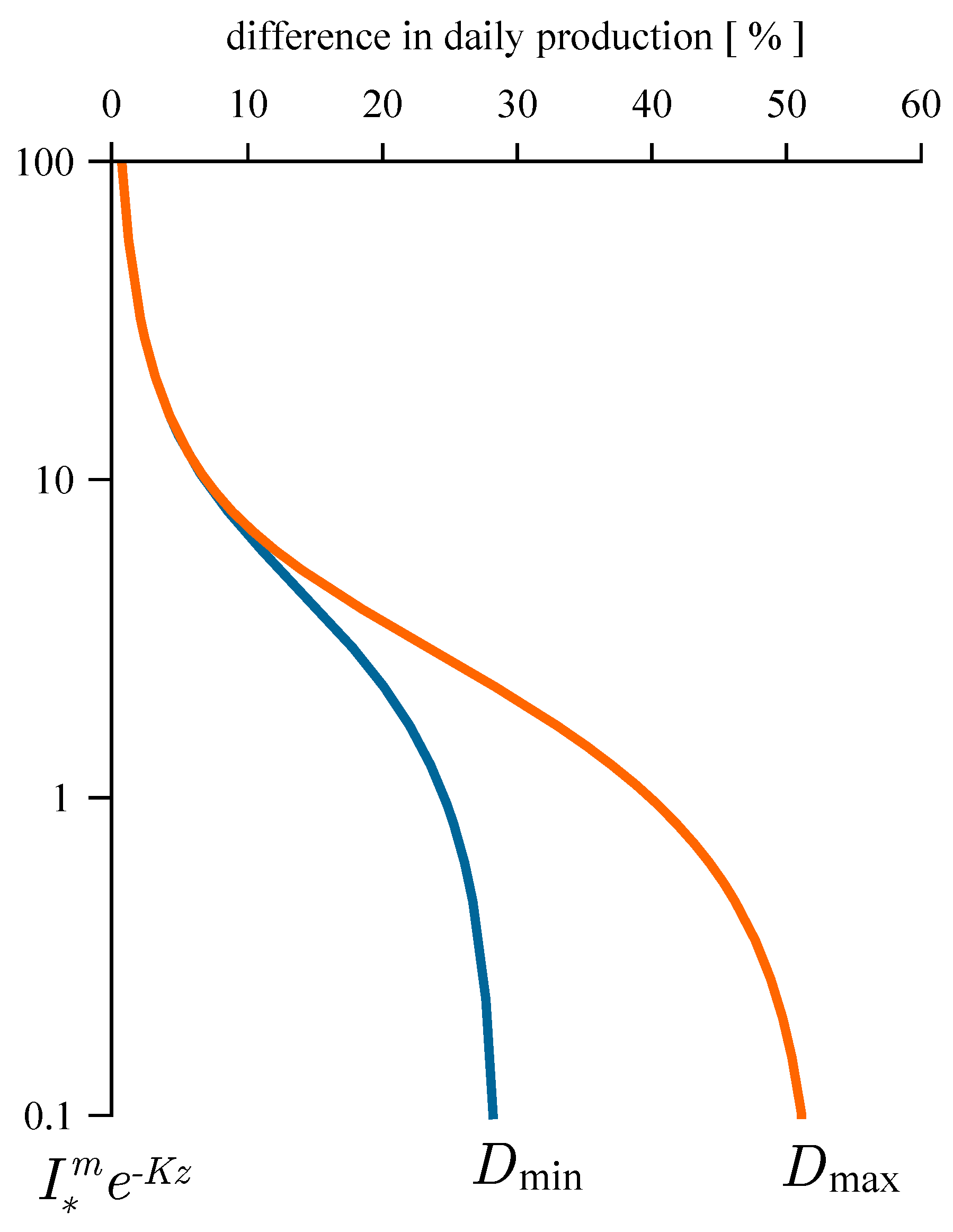
2.2. Estimating Daily Production at Depth

Daily production at depth $P_T(z)$ is defined as the amount of carbon assimilated per cubic metre during day length D. There are several ways of quantifying daily production in the ocean. The first, and most straightforward way, is to measure daily production at sea directly by incubations lasting from sunrise till sunset [7]. The second way is to estimate the photosynthesis light relation experimentally [23] and integrate it over day length, normally done with a mathematical model. The third approach is to carry out incubations shorter than day length, recover average production and extrapolate it over day length.

Typically, such shorter incubations are carried out around noon, when production is at its highest value for the day and probably light-saturated at the surface. By extrapolating average production measured during this period over day length, we might in fact be assuming saturation during the entire day length. This is known not to be the case in the ocean, as light intensity is not saturating early and late in the day, and such an assumption may cause overestimation of daily production. Here, we explore a correction to this approach and explore whether the measurement protocol at Stončica station is indeed liable to overestimate primary production.

First, let us consider instantaneous production at depth z and time t during the day, and let us use the photosynthesis irradiance function of Platt et al. [16] to model it:

$$P^B(z,t)=P_m^B\left(1-exp\left(-{\alpha }^{B}I(z,t)/P_m^B\right)\right),$$

(1)

where $I(z,t)$ is irradiance at depth z at time t, ${\alpha }^B$ is the initial slope and $P_m^B$ is the assimilation number [24]. We make the assumptions of an optically-uniform water column and sinusoidally-varying surface irradiance to model $I(z,t)$:

$$I(z,t)=I_0^{m}exp(-Kz)sin(\pi t/D),$$

(2)

where $I_0^m$ is the surface irradiance and K is the attenuation coefficient [25]. Extensive details on this model can be found in Platt et al. [26] and Kovač et al. [19].

Let us now assume incubations are carried out symmetrically around noon during the incubation interval $\Delta D$. Production in this case is given as the integral of (1) over the incubation interval:

$$P_{\Delta D}(z)={\displaystyle \underset{D/2-\Delta D/2}{\overset{D/2+\Delta D/2}{\int }}}B(z)P^B(z,t)\mathrm{d}t,$$

(3)

where $B(z)$ is the biomass, here taken to be time independent. Average hourly production that would be measured during $\Delta D$ would therefore be given as:

$$\langle P(z)\rangle =P_{\Delta D}(z)/\Delta D.$$

(4)

Under the assumption that average production during $\Delta D$ is representative of average daily production, we can multiply the previous expression by D to get daily production at depth z as:

$$P_T(z)=P_{\Delta D}(z)D/\Delta D.$$

(5)

However, we already know the exact solution for daily production, given by Kovač et al. [19], to be:

$$P_T(z)=B(z)P_m^{B}D{f}_z\left(I_{\ast }^m{e}^{-Kz}\right),$$

(6)

where $I_{\ast }^m={\alpha }^B{I}_0^m/P_m^B$ is the normalized noon irradiance [26]. For the previous two expressions to be equal, we require that:

$$P_{\Delta D}(z)=B(z)P_m^B\Delta D{f}_z\left(I_{\ast }^m{e}^{-Kz}\right).$$

(7)

and this can only hold when $\Delta D=D$. Therefore, a systematic bias is introduced into daily production estimates when extrapolating (3) over day length.

The maximum and minimum magnitudes of this bias can be ascertained simply by using a model. Knowing that the incubation interval is 6 h, we can integrate (3) numerically, calculate average production using (4) and then extrapolate it linearly to get daily production by using (5). We can then compare this result with the analytical solution for daily production (6) to see how the two estimates differ under ideal (model) circumstances over a wide range of irradiance conditions. This comparison is given in Figure 1. From this Figure, we can observe that daily production is overestimated by (5) in comparison with (6). The two curves give the differences for the Julian day with the shortest day length $D_{\min }$ (blue curve) and the Julian day with the longest day length $D_{\max }$ (orange curve). For the remainder of the year, we expect the bias to lie in the interval between these two curves. As irradiance (represented by $I_{\ast }^m{e}^{-Kz}$) decreases, the difference increases, implying that incubations at greater depths are affected more than those nearer the surface.

3. Results

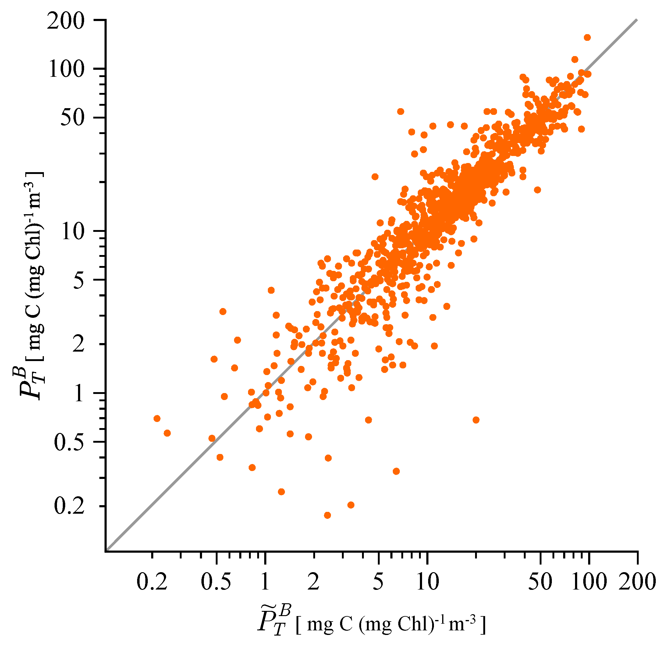
3.1. Correcting Historical Daily Production Estimates

A straightforward way of removing the bias from historical incubations at Stončica, caused by linear extrapolation of average production, would be to estimate daily production at depth by using (6). According to (6) information on biomass, day length, noon irradiance, attenuation coefficient and the photosynthesis parameters is required to estimate daily production at depth. As a starting point, we have at our disposal measured biomass and production during $\Delta D$ at a sequence of depths $z_n$, where $n=1,2,\dots ,N$. Given this set of measurements: $\tilde{B}(z_n)$ and ${\tilde{P}}_{\Delta D}(z_n)$ (where we use $\tilde{x}$ to label a measured quantity), we can reconstruct the normalized production profile ${\tilde{P}}_{\Delta D}^B(z)={\tilde{P}}_{\Delta D}(z_n)/\tilde{B}(z_n)$ and compare it with the modelled production profile given by (3). This comparison allows for extraction of a pair of photosynthesis parameters from each measured normalized production profile [9].

The assumption underlying this procedure is that the shape of the measured normalized production profile is determined by the available light and the physiological status of the phytoplankton, as expressed in the magnitudes of the photosynthesis parameters [9]. The preferred values of the photosynthesis parameters were found by an optimization algorithm that searches the parameter space and finds the optimal parameter combination for which the discrepancy between model and data is minimal. The details of the method can be found in Kovač et al. [9] and Kovač et al. [19]. For each measured profile, the method assigns one set of photosynthesis parameters for all the phytoplankton in the water column. As such, it can be applied only to normalized production profiles that are decreasing functions of depth: a direct consequence of parameter uniformity [9]. This implies that the method will not work properly for normalized production profiles that are either increasing functions of depth or for profiles that have a serpentine form.

In the entire time-series, we found a total of 185 cruises with concurrent measurements of production and chlorophyll that satisfied the vertical uniformity condition and the shape criteria. Before using these data, we excluded the outliers in ${\tilde{P}}_{\Delta D}^B(z_n)$ that were beyond three standard deviations from the mean at each depth. This procedure eliminated 70 measurements of ${\tilde{P}}_{\Delta D}^B(z_n)$. To model production at depth, we first needed to model irradiance at depth, which according to (2) requires information on $I_0^m$, K and D. Of the three, day length is most easily determined and here, we used the expression for day length from Kirk [25]. Unfortunately, surface irradiance data were not archived in the database; climatological values were used instead. However, due to the nature of the model, we can recover $P_m^B$ even without knowing the exact surface irradiance. However, for the initial slope, we can recover correctly only the product ${\alpha }^B{I}_0^m$. However, this does enable us to estimate the normalized noon irradiance $I_{\ast }^m$, a quantity that will be useful later on in the analysis. Besides $I_0^m$ and D, the next quantity required is the attenuation coefficient. To get K, we used the measured Secchi disk depth ${\tilde{Z}}_{SD}$ to express the attenuation coefficient as $K=1.44/{\tilde{Z}}_{SD}$, following Kirk [25]. The mean value of K for the entire time-series estimated in this way was 0.077 ${\mathrm{m}}^{-1}$; the median was 0.075 ${\mathrm{m}}^{-1}$; and the standard deviation was 0.014 ${\mathrm{m}}^{-1}$. Having ${\tilde{P}}_{\Delta D}^B(z_n)$, $I_0^m$ (climatology), K and D, we now have a complete set of measurements from which we can recover the photosynthesis parameters by comparing ${\tilde{P}}_{\Delta D}^B(z_n)$ with $P_{\Delta D}^B\left(z\mid {\alpha }^B,P_m^B\right)$.

We have recovered the assimilation number for 185 profiles, and its distribution is presented in Figure 2. The mean value of $P_m^B$ was 5.2; the median was 3.7; and the standard deviation was 4.0, all given in $\mathrm{mg}\mathrm{C}{(\mathrm{mg}\mathrm{Chl})}^{-1}{\mathrm{h}}^{-1}$. To the best of our knowledge, the figure presents the first estimates of the assimilation number in this region of the Adriatic Sea. Although the bulk of the values are below 5 $\mathrm{mg}\mathrm{C}{(\mathrm{mg}\mathrm{Chl})}^{-1}{\mathrm{h}}^{-1}$, a right-hand tail in the distribution is evident, implying phytoplankton populations with higher assimilation numbers are sometimes present.

Having recovered the parameters, we used them to calculate production at depth and to compare the results with measured production (Figure 3). In total, there were 1040 comparisons. The coefficient of variation was 0.87, implying that 87% of variability in measured normalized production was explained by the model, lending credence to the premise that the model provides a robust estimator of production at depth. We can now continue to the next step, which is estimation of daily production by using (6). For each incubation, we have calculated daily production using (6) and compared it with production calculated using (5). The distribution of the relative errors was found to be normal, but with a non-zero mean. On average, daily production at depth was overestimated by 20% when using (5) in comparison with (6). The standard deviation of the overestimations was 32%. These numbers quantify the bias inherent in estimating daily production, by direct application of (5), based on incubations shorter than full day length.

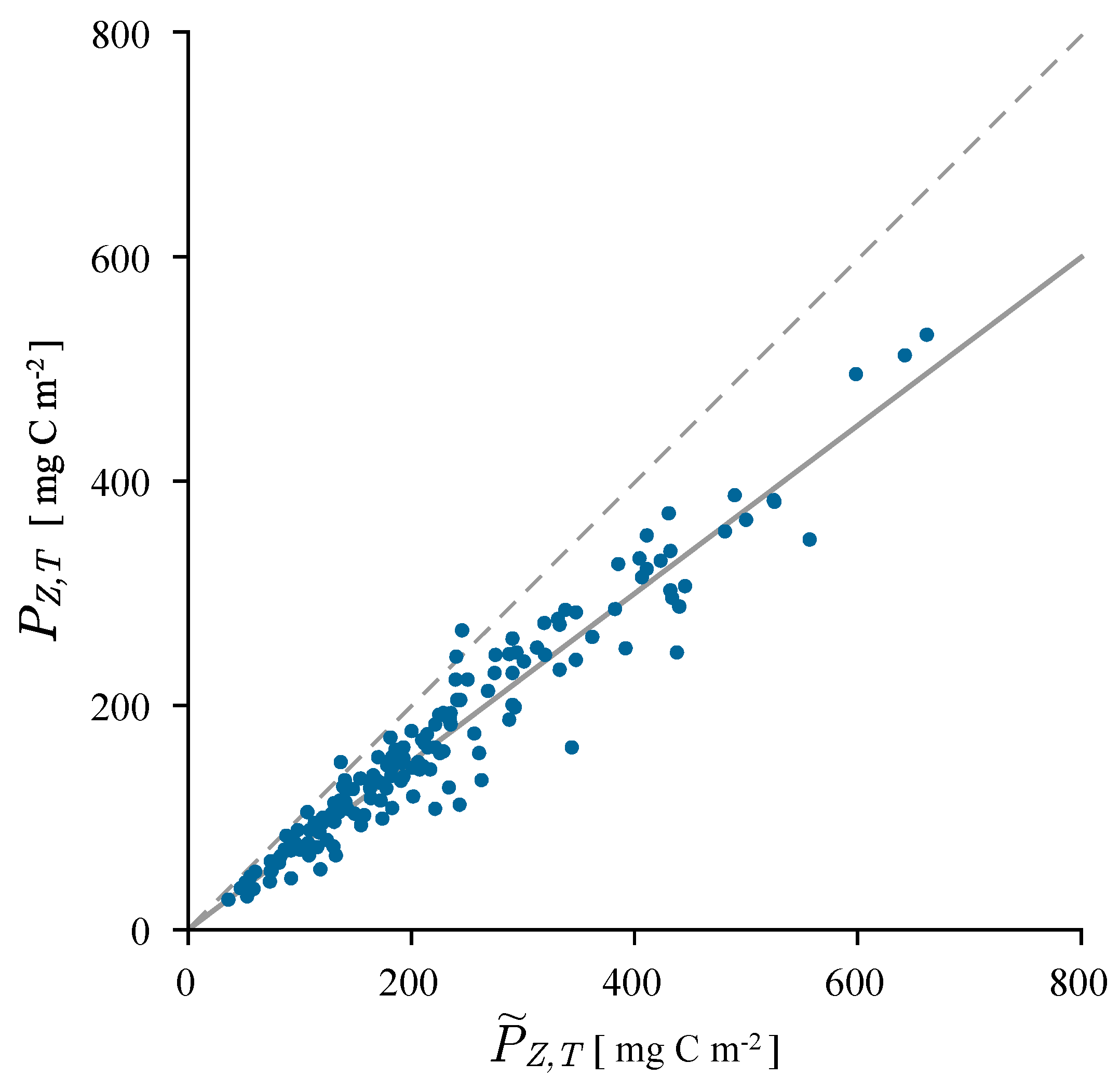
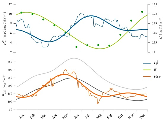
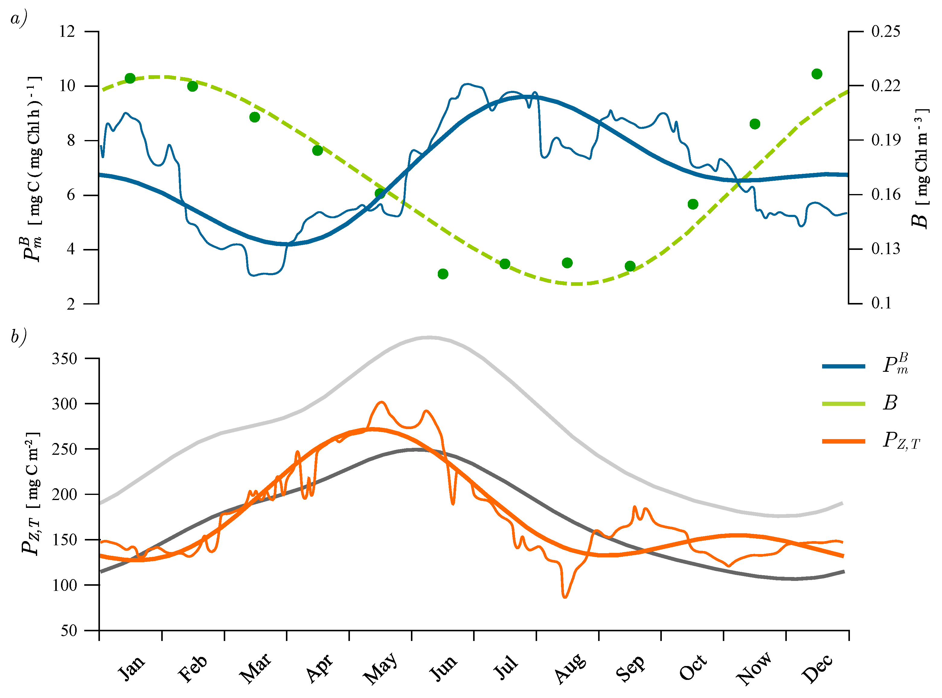
3.2. Estimating Water Column Production

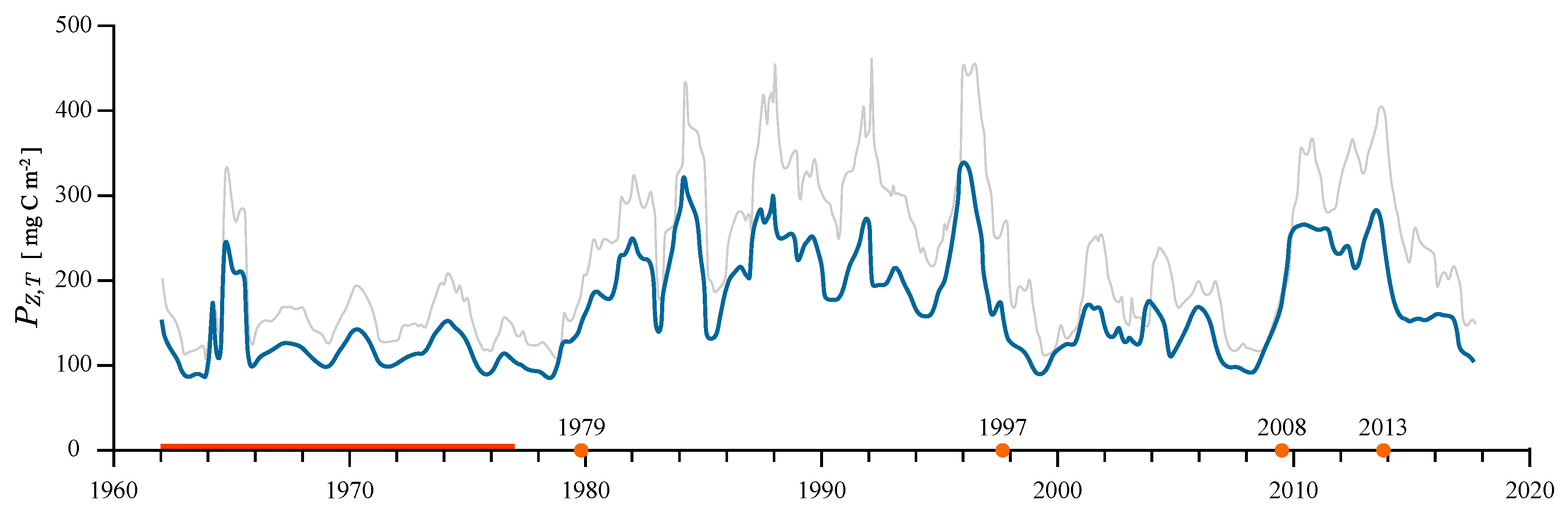
After quantifying the overestimation of daily production at depth, caused by extrapolation of average production rates at depth and over day length, we now proceed to establish the consequences it has for estimates of water column production. First, we use the definition of water column production as the integral over depth of daily production [27]:

$$P_{Z,T}={\displaystyle \underset{0}{\overset{Z_m}{\int }}}B(z)P_T^B(z)\mathrm{d}z,$$

(8)

where $Z_m$ is the water column depth. With this definition we can proceed to answer the previous question directly by calculating water column production based on (5) and on (6). Using (5), we have:

$$P_{Z,T}={\displaystyle \sum _{n=1}^N}\langle \tilde{P}(z)\rangle D\Delta z_n,$$

(9)

and using (6), we have:

$$P_{Z,T}={\displaystyle \sum _{n=1}^N}\tilde{B}(z_n)P_m^{B}D{f}_z\left(I_{\ast }^m{e}^{-\tilde{K}{z}_n}\right)\Delta z_n,$$

(10)

where $\Delta z_n$ ($n=1,2,\dots ,N$) are incremental depths around the measurement depths used for integration in the vertical. Both expressions can be normalized to biomass in which case the sums are valid for normalized water column production. The distinction between the two sums is that the first one uses measured production during the shorter-than-day length incubation interval, and the second one uses measured biomass and the estimated parameters from the measured production profiles. We treat (9) as the measured water column production and from here on label it ${\tilde{P}}_{Z,T}$, as it uses only measured quantities.

Comparing the estimates of water column production calculated by the two sums, we can estimate the bias that extrapolation of average production has on daily water column production (Figure 4). From the figure, it is evident that water column production was overestimated by (9) in comparison with (10). On average, it was overestimated by 26%, and the standard deviation of the overestimations was 25%. The thick grey line in the figure is the regression line given by:

$$P_{Z,T}=0.74{\tilde{P}}_{Z,T},$$

(11)

where we have disregarded the intercept on the y axis, as it is two orders of magnitude smaller than the average $P_{Z,T}$. This simple regression represents the correction factor for the reported water column production at Stončica station, obtained using (9).

In other words, the effect of extrapolating to D average production at depth, measured during a 6-h incubation interval around noon, to get daily production, and then integrating it over depth to calculate water column production resulted on average in a 26% overestimation of daily, water column production. This is a systematic bias, attributable not to measurement error, but to the extrapolation protocol. It can be easily rectified by following the methods demonstrated here, for cruises on which we have measured chlorophyll and production profiles. Unfortunately, both profiles were not measured on all cruises. For those cruises that did not have measured chlorophyll profiles, such that we could not estimate the photosynthesis parameters, we could still employ (11) to correct for water column production obtained by (9).

Following this approach, we could correct the time-series of water column production for errors introduced by incubation time. The time-series of annual running means of water column production is presented in Figure 5. The grey curve depicts the original time-series, obtained by application of (9), and the thick blue curve is the corrected time-series, obtained by application of (10). For the cruises on which we could not estimate the photosynthesis parameters, due to the lack of measured biomass profiles, we employed (11) instead of (10). From the figure, we see the two curves track each other well, with the blue curve consistently lower than the grey curve. The effect of the correction was linear for all the data points where we could not estimate the photosynthesis parameters, but was non-linear for the 185 cruises for which we have estimated the parameters, and subsequently water column production using (10). The total effect on the annual running means was therefore also non-linear. We see that the correction preserved much of the variability in the original time-series.

3.3. Regime Shifts

In both the corrected and the original time-series, we observe regime-like variability over the longer term. To analyse the variability in the corrected time-series, we employed a regime-shift detection method by Rodionov [28] capable of recognising distinct regimes based on the difference amongst the means in each regime. Details of the method can be found in Rodionov [28]; its implementation is publicly available at www.beringclimate.noaa.gov/regimes. The method uses a preassigned cut-off length and a significance level to test for distinct regimes, where the cut-off length determines the minimum duration of each regime and the significance level refers to the Student’s t-test for the difference in the means of two sequential regimes. For our application, we used a cut-off length of four years at the significance level of 0.01.

The method identified five regimes as displayed in Figure 5 (orange circles). From 1962–1979, average water column production was 118 $\mathrm{mg}\mathrm{C}{\mathrm{m}}^{-2}$, with one pronounced peak above 200 $\mathrm{mg}\mathrm{C}{\mathrm{m}}^{-2}$. In 1979, we observed an increase in production to a mean value of 214 $\mathrm{mg}\mathrm{C}{\mathrm{m}}^{-2}$, which persisted until 1997. In this period, there were a few peaks in production well above 200 $\mathrm{mg}\mathrm{C}{\mathrm{m}}^{-2}$ and even one above 300 $\mathrm{mg}\mathrm{C}{\mathrm{m}}^{-2}$ in 1985. In 1997, a decline in water column production marked the start of the third regime with an average production of 128 $\mathrm{mg}\mathrm{C}{\mathrm{m}}^{-2}$. This regime lasted until 2008, when a sharp rise in water column production occurred, culminating in a water column production above 300 $\mathrm{mg}\mathrm{C}{\mathrm{m}}^{-2}$. This is recognized as the fourth regime with average water column production equal to 251 $\mathrm{mg}\mathrm{C}{\mathrm{m}}^{-2}$, classifying it as the regime with highest average water column production in the series. Finally, from 2013 until the present, mean annual water column production was 154 $\mathrm{mg}\mathrm{C}{\mathrm{m}}^{-2}$. Of course, the duration of this new regime cannot be known in advance, but what is implied is that 2013 marked a probable onset of a new regime of reduced productivity.

To summarise, in

Table 1. Average values of water column production $P_{Z,T}$ ($\mathrm{mg}\mathrm{C}{\mathrm{m}}^{-2}$), assimilation number $P_m^B$ ($\mathrm{mg}\mathrm{C}{(\mathrm{mg}\mathrm{Chl})}^{-1}{\mathrm{h}}^{-1}$) and vertically averaged: chlorophyll B ($\mathrm{mg}\mathrm{Chl}{\mathrm{m}}^{-3}$), temperature T (${}^{\circ }\mathrm{C}$), dissolved inorganic nitrogen (DIN) ($\mathsf{\mu }\mathrm{mol}{\mathrm{dm}}^{-3}$) and dissolved inorganic phosphorus (DIP) ($\mathsf{\mu }\mathrm{mol}{\mathrm{dm}}^{-3}$) during each regime. Regimes are labelled by numbers in the first column and their duration given in the second column. The arrows mark a rise or a decline in average production with respect to the previous regime.

No.	Duration	${\mathit{P}}_{\mathit{Z},\mathit{T}}$	${\mathit{P}}_{\mathit{m}}^{\mathit{B}}$	B	T	DIN	DIP
1	1962–1979	118 ± 21	-	-	16.2 ± 2.8	2.04 ± 0.99	0.072 ± 0.023
2 ↑	1979–1997	214 ± 24	4.9 ± 4.1	0.19 ± 0.02	15.9 ± 3.0	1.99 ± 1.24	0.072 ± 0.048
3 ↓	1997–2008	128 ± 20	5.1 ± 3.8	0.11 ± 0.03	16.7 ± 3.0	1.67 ± 1.31	0.068 ± 0.058
4 ↑	2008–2013	251 ± 22	4.5 ± 2.6	0.21 ± 0.02	16.5 ± 3.2	1.23 ± 0.86	0.062 ± 0.082
5 ↓	2013–now	154 ± 23	4.9 ± 4.3	0.17 ± 0.01	16.8 ± 2.8	1.55 ± 0.79	0.058 ± 0.046

, we present average values of water column production, assimilation number and chlorophyll during each regime. Since chlorophyll measurements began at Stončica station in 1977 and the first regime in production ended in 1979, we had very few data on chlorophyll and consequently also on the assimilation number for the first regime, and therefore did not present them. From Table 1, we observe that the average assimilation number is consistent across the regimes, implying that the rate of carbon assimilation is not the cause of changes in water column production. However, we observe that average chlorophyll does change from regime to regime, almost halving from 1997–2008 in comparison with the regimes before and after it. For reference, we also present in Table 1 average values of temperature, dissolved inorganic nitrogen and phosphate. These are water column averages additionally averaged in time over each corresponding regime.

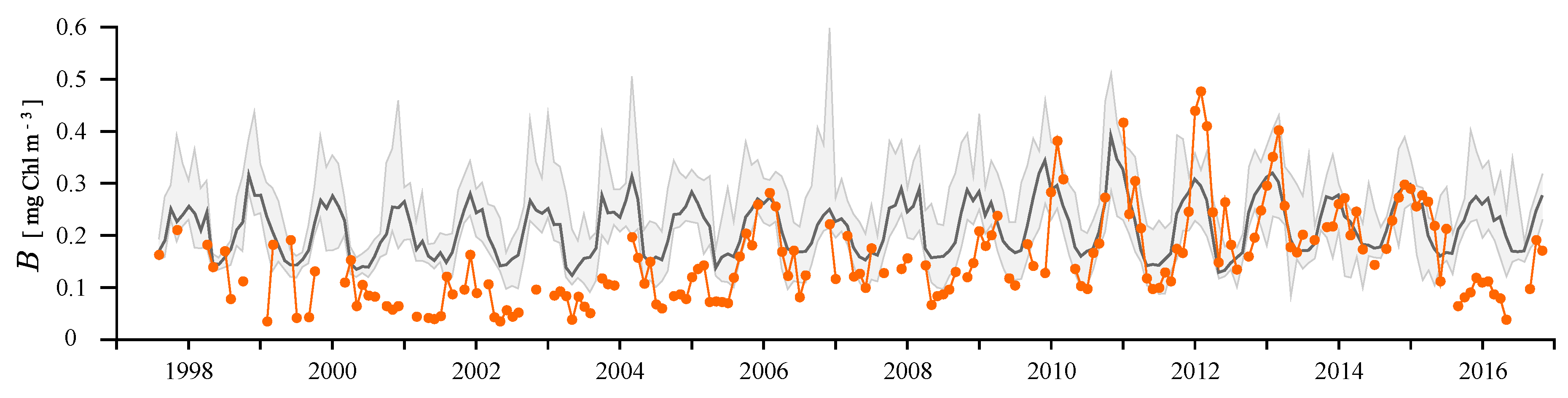
3.4. Remote Sensing Application

The recovered assimilation numbers and the demonstrated ability of the model to calculate production at depth accurately, using the recovered parameters (Figure 3), enable us now to estimate primary production using remotely-sensed data. Our goal is to estimate the seasonal cycle of primary production at this station and to compare it with observations. To achieve this goal, we need to select a model for water column production, and we opted for the canonical solution of Platt et al. [26], which gives $P_{Z,T}$ as:

$$P_{Z,T}=\frac{B{P}_m^{B}D}{K}\left[f(I_{\ast }^m)-f(I_{\ast }^m{e}^{-K{Z}_m})\right],$$

(12)

where $f(I_{\ast }^m)$ is a known function, B is assumed to be vertically uniform and $Z_m$ is the bottom depth in our case. This model has been demonstrated to be robust for modelling water column production in many and diverse applications, not limited solely to remote sensing [7,29,30,31]. With it, we proceed to calculate water column production on each Julian day and thereby construct the seasonal cycle of $P_{Z,T}$.

The key variable available to us from the satellite is the chlorophyll concentration. The Version 3.1 of the European Space Agency’s Ocean Colour Climate Change Initiative (OC-CCI) [32,33] was acquired in this study. The monthly Level 3 remotely-sensed surface chlorophyll measurements from the OC-CCI dataset were acquired at 4-km resolution from www.esa-oceancolour-cci.org. We extracted the data around the Stončica station in the Adriatic Sea for the period of 1997–2016. The OC-CCI product consists of bias-corrected error-characterised mission-merged chlorophyll-a data from the Sea-Viewing Wide Field-of-View Sensor (SeaWiFS), Moderate Resolution Imaging Spectroradiometer (MODIS), Medium Resolution Imaging Spectrometer (MERIS) and Visible Infrared Imaging Radiometer Suite (VIIRS) satellite sensors. In approaching their task, the OC-CCI team considered that the utility of ocean-colour data streams, especially in the context of research on climate change, is related not just to the data themselves, but also to the excellence of the algorithms used to retrieve optical and biogeochemical ocean properties from the spectral radiances incident at the satellite sensor. The algorithms chosen from those available should be the best possible for their stated purpose, namely detection of perturbations in properties of the ocean ecosystem as a result of climate change. The pelagic ecosystem has many degrees of freedom to respond to a change in climate, such as modifications in regional distributions of the abundance and kinds of phytoplankton, and in their phenology. The preferred algorithms would be able to distinguish between amount and type of phytoplankton; would not change when the climate changed; and would be independent of assumptions valid only under climatic conditions of today. Using these considerations, they identified a suite of qualitative traits that algorithms ideal for climate-change studies would possess. Of course, these traits would complement the stringent quantitative characteristics of precision, accuracy and stability in the data over secular scales. Existing algorithms were examined for their ability to meet the identified criteria, and where they should be improved further, as required [33]. The uncertainties in the OC-CCI products have been established on a per-pixel basis by comparison with an extensive database of in situ observations and assignment of uncertainties according to an optical classification scheme [34]. We also refer the reader to the OC-CCI Product User Guide at www.esa-oceancolour-cci.org/?q=webfm_send/318 for more extensive information on data processing, sensor merging and uncertainty quantification.

Time-series of the in situ chlorophyll are shown in Figure 6 along with the monthly satellite-derived chlorophyll data. In the figure, the vertically-averaged in situ chlorophyll concentration is given in orange, with the minimum to maximum remotely-sensed chlorophyll range given in light grey shading and the average given in dark grey. We present the vertically-averaged chlorophyll because it occurs in the canonical solution (12) to model the seasonal cycle. As such, we are not comparing in situ and satellite data, but only exploring the extent to which satellite-derived chlorophyll may be considered as being representative of water-column average chlorophyll.

In Figure 6, the range of the measured chlorophyll concentrations is captured well by the remotely-sensed data. However, we note that, in the early years of the satellite data, particularly from 1998–2008, the differences between the satellite data and the vertically-averaged in situ data were higher, suggesting a possible change in the relation of surface chlorophyll to chlorophyll at depth around 2008, at the time of the regime shift in primary production (Table 1). The variability in the in situ averaged chlorophyll was matched well by the remotely-sensed data for the rest of the time-series. We have tested the differences statistically, and the distribution of the relative errors in the period till 2008 was positively skewed with a non-zero mean, whereas the distribution of the relative errors after 2008 was normally distributed. These results indicated that the satellite data during the 1997–2008 regime might not be a good substitute for in situ depth-averaged chlorophyll, for use in the uniform-biomass-water column primary production model. This however does not imply that the remotely-sensed chlorophyll is inadequate for more complex models, which resolve the vertical structure in biomass.

Nevertheless, to make full use of the remotely-sensed data, we estimated the seasonal cycle of biomass from the remotely-sensed minimal chlorophyll concentrations (lower bound of shaded curve in Figure 6) for use in (12). Using minimum chlorophyll concentrations implies our estimate of $P_{Z,T}$ will be conservative with respect to biomass. Monthly, average biomass is given in Figure 7a (green points). Onto the monthly averages, we further fitted a sum of two sine functions superimposed onto a mean (Figure 7a, dashed green line). The first sine had a one-year period, and the second had a half-year period:

$$B(j)=0.168-0.055sin(2\pi j/365-4.016)-0.005sin(4\pi j/365+4.985),$$

(13)

given in $\mathrm{mg}\mathrm{Chl}{\mathrm{m}}^{-3}$, where $j=0,1,2,\dots ,365$ is the Julian day. This representation of the seasonal cycle of biomass enables us to have an estimate of biomass on each Julian day, which is required to calculate $P_{Z,T}$, also on each Julian day.

To calculate the seasonal cycle of $P_{Z,T}$ following (12), we also need information on $P_m^B$ on each Julian day. For this, we used the 185 recovered values of $P_m^B$ to construct the seasonal cycle. On each Julian day, we calculated the mean value of $P_m^B$ from the cruises that fell in the interval of 15 days prior and 15 days after a given Julian day (Figure 7a, thin blue curve). Onto this, we fitted a sum of two sines, and in this way, we have estimated the seasonal cycle of the assimilation number (Figure 7a, thick blue curve). Again, the first sine has a one-year period, and the second has a half-year period:

$$P_m^B(j)=6.8-1.9sin(2\pi j/365+0.6)+1.2sin(4\pi j/365+1.1),$$

(14)

given in $\mathrm{mg}\mathrm{C}{(\mathrm{mg}\mathrm{Chl})}^{-1}{\mathrm{h}}^{-1}$, where $j=0,1,2,\dots ,365$ is the Julian day.

We now have an estimate of $P_m^B$ on each Julian day, which we can use in (12). At the onset of the year, the assimilation number was declining, reached a minimum during March, then began to increase, reached a maximum during July and August, after which it declined to its winter value. The observed seasonal cycle of $P_m^B$ implies its periodicity will have a significant effect on the calculation of the seasonal cycle of water column production. If a seasonal signal had not been observed or if sufficient data had not been available to estimate it, as a first order estimate, we could have used the year-long average value of the assimilation number.

Of the remaining variables required in (12), day length D is easily calculated: we used the expression for day length from Kirk [25]. For the attenuation coefficient, we used a single fixed value: the year-long mean, and for noon irradiance, we used the climatology. We should note here that the $f(I_{\ast }^m)$ function requires information on ${\alpha }^B$, which was unavailable to us, due to the lack of archived $I_0^m$, which could have been used to estimate it. However, we estimated ${\alpha }^B$ from the climatological noon irradiance, for each cruise on which we had $P_m^B$, as ${\alpha }^B=I_{\ast }^m{P}_m^B/I_0^m$. With ${\alpha }^B$ estimated in such a way, we did not observe a pronounced seasonal cycle, so instead, we calculated its mean, equal to 0.124 $\mathrm{mg}\mathrm{C}{(\mathrm{mg}\mathrm{Chl})}^{-1}{(\mathrm{W}{\mathrm{m}}^{-2})}^{-1}{\mathrm{h}}^{-1}$, which we then used in (12) on each Julian day. Although not ideal, it is the best estimate of ${\alpha }^B$ we could find.

With the required parameters now accessible on each Julian day, we calculated daily water column production using (12), and the results are displayed in Figure 7b. The light grey curve represents $P_{Z,T}$ calculated with the climatological noon irradiance, and the dark grey curve represents $P_{Z,T}$ calculated with half the climatological noon irradiance. This reduction represents the effect of cloud cover [15] and as such gives the lower limit on production that would be achieved by using remotely-sensed chlorophyll. In principle, cloud cover removes the direct component of solar radiation, leaving only the diffuse component, which corresponds to a reduction of about 50% in total irradiance. Therefore, by keeping the same chlorophyll and reducing light intensity in such a way, the effect of cloud cover on primary production was simulated. Following Platt et al. [15], these two calculations represent the possible range of water column production that can be calculated from climatological data on irradiance.

On top of these estimates, we further present the seasonal cycle of daily production, based on water column production estimated by using (10) and (11), i.e., the corrected measured water column production $P_{Z,T}$ (Figure 7b, orange). From the figure, we see the seasonal cycle of corrected $P_{Z,T}$ was consistent with that calculated based on remotely-sensed chlorophyll (grey curves). Water column production was lowest during winter, started increasing in spring and reached a maximum in May/June, after which it declined to its winter values. The maximum in production based on remotely-sensed chlorophyll lagged approximately a month behind the maximum in corrected $P_{Z,T}$. This may be due to $P_{Z,T}$ being estimated from all the available data from 1962–2017, whereas remotely-sensed $P_{Z,T}$ was based on chlorophyll only from 1997–2016 and $P_m^B$ from the 185 cruises. The two may not agree fully because the seasonal cycle of biomass or production, or both, might have changed over time through one or more regime shifts. In fact, Marasović et al. [6] have already reported evidence of changes in the seasonal cycle at this station. Irrespective of these changes, the lower estimate of $P_{Z,T}$ based on remotely-sensed chlorophyll (dark grey) did match the corrected $P_{Z,T}$ in magnitude. The upper estimate of $P_{Z,T}$ based on remotely-sensed chlorophyll (light grey) was not reached by the measured $P_{Z,T}$. This is to be expected since it represents the upper bound on $P_{Z,T}$.

It is important to highlight the essential difference between the two estimates and the measured $P_{Z,T}$. Measured production was determined under natural irradiance conditions at sea on the day of measurement, and that production was then averaged to calculate the seasonal cycle of $P_{Z,T}$. However, the calculations based on (12) used the average seasonal cycle of irradiance to construct the seasonal cycle of water column production. This procedure eliminates in advance any variability caused by fluctuations in production due to reduction in irradiance caused by cloud cover. The same is true for the rest of the variables that were represented by smoothly-varying functions of time; some variability that was observed in measured $P_{Z,T}$ may be absent from estimates based on (12).

4. Discussion

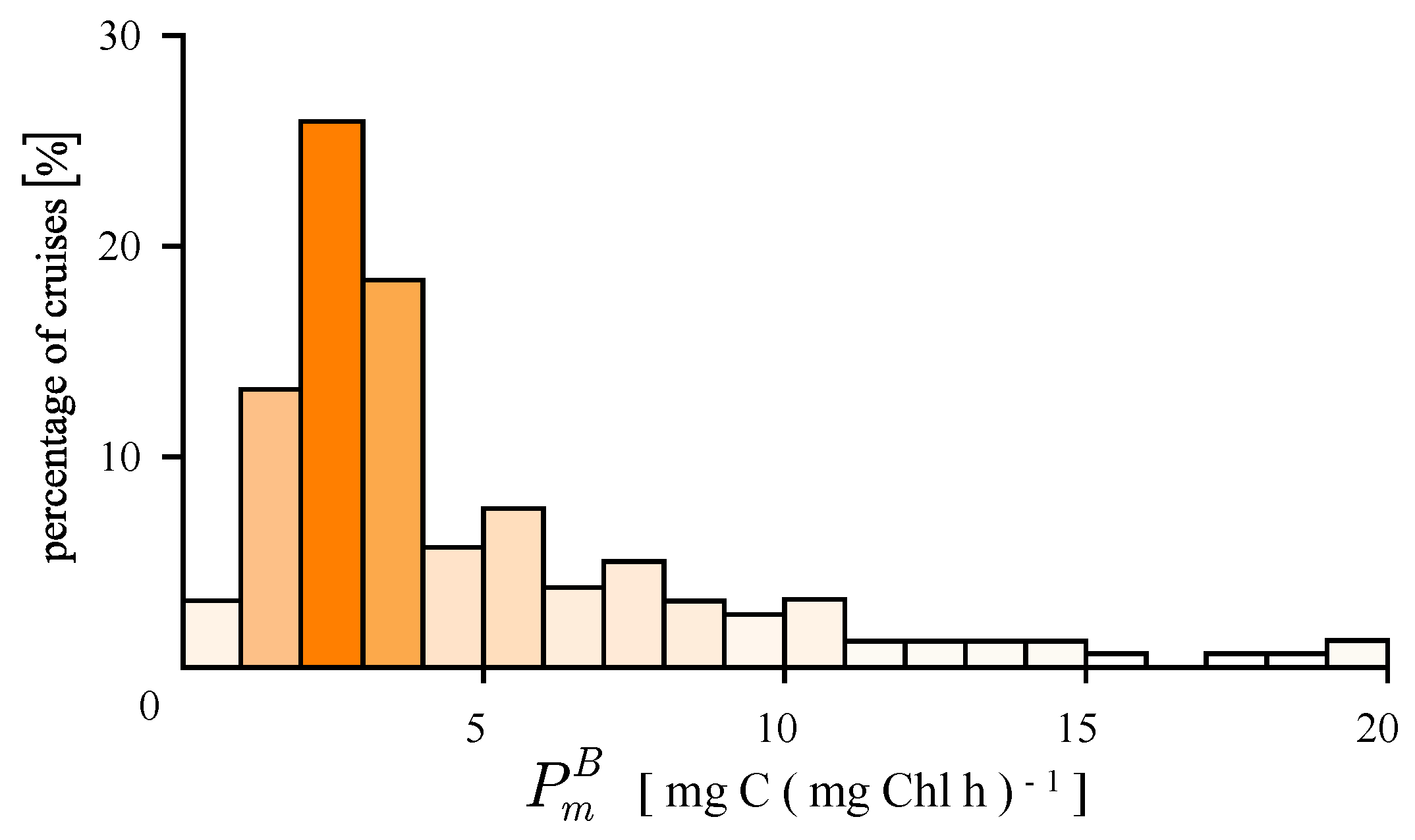
4.1. Recovered Assimilation Numbers

Photosynthesis includes both primary light-dependent and secondary light-independent reactions [25]. Under low light conditions, photosynthesis is a linear function of irradiance with a slope ${\alpha }^B$ (initial slope), dependent on the number of photosynthetic reaction centres and their absorption cross-section [24,35], whereas at light saturation, it is dependent on the capacity of secondary reactions (Calvin cycle) and proceeds at a rate $P_m^B$, recognized as the assimilation number [36,37]. The ratio of the two parameters $I_k=P_m^B/{\alpha }^B$ is a useful index for light saturation [16,38]. The decrease of photosynthesis at very high light intensity due to photoinhibition could also be observed [39,40]. However, at sea, photoinhibition is mostly limited to the upper portion of the water column, where light intensity is highest, and therefore, its influence on water column production is expected to be of minor importance. This is also corroborated by the fact that the errors of the model for production at depth are distributed normally (Figure 3), even though photoinhibition was not modelled. The above-mentioned characteristics of photosynthesis are readily estimated from photosynthesis light experiments conducted under controlled light conditions [24,41]. They can also be observed from measured production profiles [42].

Following the approach of Kovač et al. [9] we have estimated the assimilation number from 185 measured normalized production profiles. The mean value of the assimilation number was found to be 5.2 $\mathrm{mg}\mathrm{C}{(\mathrm{mg}\mathrm{Chl})}^{-1}{\mathrm{h}}^{-1}$, which is about 20% of the theoretical maximum of 25 $\mathrm{mg}\mathrm{C}{(\mathrm{mg}\mathrm{Chl})}^{-1}{\mathrm{h}}^{-1}$, determined by Falkowski [36]. According to Karl et al. [43], assimilation numbers in natural populations are mostly from 10–50% of the theoretical maximum, suggesting reduced photosynthetic activity due to limitations of light, temperature and nutrients. Photosynthetic rate dependence on these factors in the ocean is a result of a series of complex processes operating at a wide range of spatial and temporal scales [25,44]. In addition, phytoplankton abundance and community composition influence the fate of light through pigment-specific absorption. As a result, the assimilation number measured under natural conditions is considered as representative of a particular region only [45].

In comparison with other regions and studies, the mean value of the assimilation number obtained in this study (5.2 $\mathrm{mg}\mathrm{C}{(\mathrm{mg}\mathrm{Chl})}^{-1}{\mathrm{h}}^{-1}$) is very similar to other values reported worldwide: Bedford Basin, Nova Scotia 5.48, Woods Hole 5.7, Southern Long Island 4.6, St. Margaret’s Bay, Nova Scotia 5.0, all given in $\mathrm{mg}\mathrm{C}{(\mathrm{mg}\mathrm{Chl})}^{-1}{\mathrm{h}}^{-1}$ (see Harrison and Platt [46] and the references therein). Lower assimilation numbers were recorded in the Southern Baltic 3.31 [47], Fraser River Estuary 2.1 [48], Southern Ocean 0.9 [49], all given in $\mathrm{mg}\mathrm{C}{(\mathrm{mg}\mathrm{Chl})}^{-1}{\mathrm{h}}^{-1}$, while higher were recorded for Hawaii 6.3–15.5 $\mathrm{mg}\mathrm{C}{(\mathrm{mg}\mathrm{Chl})}^{-1}{\mathrm{h}}^{-1}$ by Laws et al. [50]. Concerning the Mediterranean, Videau et al. [51] reported values from 0.2–5.0 for the Almeira-Oran front in the south-western Mediterranean, Latasa et al. [52] reported $3.48\pm 2.02$ for the north-western Mediterranean and Morán and Estrada [53] reported values from 0.59–6.25 for the Alboran Sea, all given in $\mathrm{mg}\mathrm{C}{(\mathrm{mg}\mathrm{Chl})}^{-1}{\mathrm{h}}^{-1}$. The values reported by these authors are consistent with the ones reported in this work. It is worth nothing that Gasol et al. [54] have also estimated the seasonal cycle of the assimilation number from 12 years of monthly photosynthesis-irradiance measurements in Blanes Bay. By comparing their Figure 5a with Figure 7a, we see that the seasonal cycles are consistent, with maxima and minima occurring at the same time of the year. However, all of the above estimates were obtained using a different methodology, the previously-mentioned controlled-light experiments on the photosynthesis irradiance curve [24].

Estimates based on the same approach to that used in this work have been made so far on two stations. These are the Hawaii Ocean Time-series (HOT) [9,19] and the Bermuda Atlantic Time-series Study (BATS) [55] datasets. For both HOT and BATS, the initial slope and the assimilation number have been estimated, thanks to those time-series having archived measured surface irradiance. Not having archived measured surface irradiance at Stončica station prevented the estimation of the initial slope. However, the assimilation number has been estimated, and we can compare the values obtained at the three stations. For both HOT and BATS, the bulk of the $P_m^B$ values are above 5 $\mathrm{mg}\mathrm{C}{(\mathrm{mg}\mathrm{Chl})}^{-1}{\mathrm{h}}^{-1}$, whereas for Stončica, the bulk are below 5 $\mathrm{mg}\mathrm{C}{(\mathrm{mg}\mathrm{Chl})}^{-1}{\mathrm{h}}^{-1}$. The values of $P_m^B$ at HOT are mostly concentrated in the interval from 5–10 $\mathrm{mg}\mathrm{C}{(\mathrm{mg}\mathrm{Chl})}^{-1}{\mathrm{h}}^{-1}$, whereas at BATS, the values of $P_m^B$ are more spread out, in the interval from 5–15 $\mathrm{mg}\mathrm{C}{(\mathrm{mg}\mathrm{Chl})}^{-1}{\mathrm{h}}^{-1}$.

For the entire photic zone, average daily water column production at HOT was 436 $\mathrm{mg}\mathrm{C}{\mathrm{m}}^{-2}$, and at BATS, it was 441 $\mathrm{mg}\mathrm{C}{\mathrm{m}}^{-2}$ [56], whereas average water column production at Stončica was 160 $\mathrm{mg}\mathrm{C}{\mathrm{m}}^{-2}$, roughly 2.7-times smaller than HOT or BATS. One could argue that smaller water column production at Stončica station results from its being only 100 meters deep, whereas HOT and BATS are open ocean stations. This is only a partial reason at best; if it were the sole reason, we would expect a similar range on the distribution of the assimilation number. Since the distributions of $P_m^B$ differ, both in magnitude and in shape, we infer the productivities differ for physiological reasons, which are linked to community structure. However, the seasonal cycles at the three stations are quite similar (see Figure 6 in Kovač et al. [19] and Figure 6 in Kovač et al. [55]). At Stončica, the highest primary production occurs in spring (Figure 7b) during diatom dominance due to extended daylight and sufficient nutrients. During summer stratification, nutrients in the euphotic layer are consumed, limiting production. The second, smaller peak in autumn is the result of water column mixing, due to cooling of the surface layer, which subsequently leads to nutrient enrichment and higher production. This cycle, driven by available light and nutrients, is characteristic of temperate seas [57].

In the presentation of the seasonal cycle of the assimilation number in Figure 7a, it is evident that the highest values are observed during the summer period, whereas the lowest are observed at the colder time of the year. This pattern results from the differences in light availability, temperature and phytoplankton community structure. Generally, phytoplankton photosynthesis increases quasi-linearly (in fact, hyperbolically) with light intensity until reaching maximum photosynthesis at saturating intensity ($P_m^B$). The light intensity needed to reach maximal photosynthesis varies among different taxonomic groups. According to Ryther [18], dinoflagellates require much higher illumination and show lower inhibition at intensities above the saturating intensity in relation to other taxonomic groups. In the research area, unarmoured dinoflagellates and unicellular cyanobacteria Synechococcus prevail in summer, whereas coccolithophorids dominate in winter [58]. During the spring, diatoms prevail, mostly Chaetoceros species in surface layers and Pseudo-nitzschia spp. and Leptocylindrus danicus in subsurface layers [58]. This seasonal distribution of phytoplankton taxa is influenced by the changes in environmental conditions that in different seasons favour the growth of different taxonomic groups. According to Ninčević [59], relatively high assimilation numbers during the colder part of the year could be attributed to phytoplankton size fractions >10 $\mathsf{\mu }\mathrm{m}$, while size fractions <10 $\mathsf{\mu }\mathrm{m}$ showed higher photosynthetic activity during the warmer time of the year, which is a reflection of the seasonal composition of the phytoplankton community. The investigated area is characterized by the dominance of picoplankton (>60%) in total phytoplankton carbon [58]. Furthermore, temperature affects the enzyme-induced secondary reaction of photosynthesis and thus affects the assimilation number.

Higher assimilation numbers during summer, compared with spring, could be explained by greater pigment packaging and self-shading in bigger cells, such as diatoms Pseudo-nitzschia spp. and Leptocylindrus danicus, in comparison with the smaller nanoplankton cells, which prevail in summer during stratification. According to Kirk [60], the package effect becomes significant for cells bigger than 10 $\mathsf{\mu }\mathrm{m}$. These findings are in accordance with a decline in the assimilation number during a period of diatom dominance.

4.2. Remotely-Sensed Chlorophyll

In addition to the seasonal cycle based on in situ measured variables, we have also looked at the remotely-sensed seasonal cycle of biomass. In Figure 6, we notice that during a short period from 2010–2014, the amplitude of the seasonal cycle is more pronounced. In this period, the variability in the remotely-sensed record of chlorophyll matches the in situ record. Prior to 2010, the annual mean and the amplitude of the seasonal cycle of in situ chlorophyll are smaller. However, the amplitude and the mean of the seasonal cycle of remotely-sensed chlorophyll are stable over the entire time-series. Further, the period from 1997–2008 was identified as a low productivity regime, and here, we see it is also characterized by lower in situ chlorophyll. After 2008, in situ chlorophyll increases and so does production. However, the remotely-sensed chlorophyll does not capture this behaviour. Similarly, Civitarese et al. [61] reported no significant interannual or decadal variability when analysing SeaWiFS chlorophyll concentrations time-series over the Central Adriatic, highlighting the need for in situ measurements in parallel with remote sensing measurements. The two complement each other, one providing superior spatial and temporal coverage, the other more precise local information.

However, this work did not set out to validate the satellite signal, but to provide an overall visual comparison between the integrated values in the water column, versus the surface satellite-derived concentrations. The full problem of comparison is complex and cannot be resolved simply, even with site-specific algorithms, since these can hardly be tuned well for every season in a single area. Water colour signal recorded by the satellites, generally interpreted as chlorophyll concentration, often correlates well with in situ chlorophyll data in the open ocean. However, even at the Stončica station, there are spectral signals other than chlorophyll that can influence the spectral signature of surface waters, and many phytoplankton pigments show similar spectral properties to chlorophyll [62].

Pigments other than chlorophyll have been measured in the open South Adriatic, although in low concentrations [63]. These are related to species generally present over the whole of the Adriatic. Depending on the phytoplankton species and the phases in the their life cycle, spectral signals from various pigments may contribute to the chlorophyll signal, leading potentially to overestimation of chlorophyll concentrations as determined from satellite data. If these change over time, as is hinted at by the shifts in production, but the algorithm remains the same, discrepancies such as seen in Figure 6 may arise.

Another reason for the discrepancy between the two types of data comes from different coloured substances in the sea, most of which are products of degraded pigments and disintegrated cells. These have similar spectral properties to a yellow substance, attenuating strongly at shorter wavelengths [64]. Such substances are present in the water column, from cells dying and sinking to the bottom. Strong winds during cold periods may mix up the sediment from the bottom, bringing these substances to the euphotic zone, which may then make them visible to satellite optical sensors. It was shown for the Adriatic that large differences between in situ and satellite chlorophyll coincided with strong wind events, particularly in the Northern Adriatic [65]. The Stončica station, being 100 $\mathrm{m}$ deep, is situated over the shelf where the water column is typically well mixed during the cold season. This would allow bottom sediments, some of which are coloured, to come to the surface at this time of year and influence the spectral signal reaching the satellite.

Regardless of the difference in what the satellite is measuring (water leaving radiance from pixels of several hundred metres to kilometre size) and one litre of water sampled for laboratory chlorophyll analysis, spatial inconsistency is not an issue for this area. The investigated area is considered open sea and homogeneous in an oceanographic sense at scales of tens of kilometres around the station. Similarly, temporal consistency can be discussed in a simple way, by noting that in situ sampling for chlorophyll was always performed at the same time of the day at around 9:00. This time of measurement should match the satellite overpass time as closely as possible if comparison of individual measurements were done, but here, daily in situ measurements are related to whole monthly range of daily satellite measurements (Figure 6). Analysing match-ups and developing a local algorithm for this area is a potential course for future research.

4.3. Long-Term Changes

Looking now at longer time scales, the detected regimes and their distinct longevity provide evidence that the time-series is not stationary, in the sense of not having time-independent statistical properties, such as mean and variance. This is interesting from the point of view of ergodicity, which can be used in this context in the following way. We can ask whether primary production has the same behaviour averaged over time as it would have averaged over space. In the language of oceanography, can a sufficiently long time-series serve to provide information on the natural variability of primary production in the province in which the station is located. If so, measuring at a single station for a sufficiently long time would provide all the possible information on the province. Therefore, changes in the properties of the time-series would directly implicate other possible changes taking place elsewhere in the province. The standard practice in oceanography is to assume implicitly that this assumption holds. If it were true, a change at the station would reflect a change, or changes, in the wider area around the station.

Stončica station is situated in the Central Adriatic near the island of Vis. Here, the waters are oligotrophic, highly transparent and well aerated, with low primary productivity, low chlorophyll and low nutrient concentrations (Table 1). The area is influenced more or less constantly by the East Adriatic Current, which brings waters from deeper layers of the South Adriatic. Due to bathymetric characteristics, these waters are forced to upwell in the wider area of the Palagruža Sill and also in the area around the station. Sometimes, during the stratified season and under favourable wind conditions, this area of the Central Adriatic is also influenced by surface currents from the east coast or even from the west coast [66,67], both bringing fresh surface water from adjacent coasts. However, this occurs sporadically and does not have a major role in long-term dynamics.

Study of the long-term dynamics at this station has a long history. It started at the time of Buljan [68], who showed strong decadal variability in salinity and linked it to the Eastern Mediterranean water inflow into the Adriatic. He hypothesized how these waters, which are more nutrient rich than the Adriatic waters, would act to increase primary production via nutrient enrichment and that periods of higher production would coincide with periods of increased influx of Mediterranean waters. He called these events the Adriatic ingressions. Since then, various studies on long-term dynamics have been conducted, such as: Marasović et al. [6], Grbec et al. [11], Vilibić et al. [69], to name a few.

The first to study and precisely quantify regimes in primary production in the Adriatic were Grbec et al. [11], who analysed the uncorrected time-series (grey curve in Figure 5) in the period up until 2002. The regimes they obtained correspond to the ones reported in this work (see Figure 3 in Grbec et al. [11]). The authors observed that the first regime corresponded to lower winter air temperatures in the North Adriatic and higher sea temperature in deeper layers at the investigated Stončica station. This corresponds to stronger intrusions of the Mediterranean warmer and nutrient richer water, in comparison with Adriatic water. A reversal of this relation corresponds with the timing of the shift in primary production in 1979. Grbec et al. [11] have found the air temperature in the North Adriatic during the second regime to be above average, but sea temperature in deeper layers at the Stončica station to be below average. This regime corresponds to weaker intrusions, with colder and less salty Adriatic waters in deeper layers, since the water is not replenished by warmer and more saline Mediterranean water.

In two complementary studies on longer time scales, variability of the circulation and water exchange in the South Adriatic was described by the Adriatic-Ionian Bimodal Oscillating System by Gačić et al. [70] and by Civitarese et al. [61]. In this paradigm, the influx of water masses from the Ionian into the Adriatic is determined by whether the upper-layer Ionian circulation is cyclonic or anticyclonic. Cyclonic circulation favours influx of Levantine intermediate water, whereas anticyclonic favours influx of modified Atlantic water. As these waters have different nutrient characteristics, they exert different influences on primary production in the Adriatic.

However, contrary to Buljan [68], Civitarese et al. [61] argue that higher production in the South Adriatic would be caused by modified Atlantic waters and not by the Eastern Mediterranean waters. The reason is that during cyclonic circulation in the Northern Ionian Gyre, the nutricline is depressed at the border of the gyre, and therefore, nutrient-deprived waters enter the South Adriatic through the Otranto Strait. During anticyclonic circulation, modified Atlantic waters with increased nutrients enter the South Adriatic because the nutricline is uplifted along the gyre periphery. Gačić et al. [70] demonstrated that the circulation in the Northern Ionian reverses on a decadal time scale, and they provided a mechanistic explanation for the reversal. In 1997, a reversal from anticyclonic to cyclonic circulation in the Northern Ionian Gyre was reported [61]. Following the previous argument, this should have caused a decline in production in the Adriatic Sea. Strikingly, a regime shift in primary production was detected in the same year (Figure 5), with a fall in production occurring, as predicted on the basis of the argument of Civitarese et al. [61] concerning the circulation in the Northern Ionian. Further research is needed here.

5. Conclusions

Since 1962, primary production has been measured at Stončica station in the Central Adriatic during six-hour intervals around noon and average measured production extrapolated linearly to calculate daily production. In this work, it was demonstrated that such a procedure is biased and tends to overestimate daily production. The overestimation was found to be on average 20% for production at depth and 26% for water column production (Figure 4). Using a non-linear production model, this bias was removed from the historical estimates of daily production.

Subsequently, a time-series of annual running means of corrected water column production was constructed, and it was observed to be non-stationary. Distinct regimes in water column production time-series have been identified and average water column production of each regime quantified precisely with the method of Rodionov [28] (Figure 5). The duration of each regime was on the order of a decade, and such long regimes could have been detected only by virtue of the length of the time-series. The existence of regime shifts in daily, water column primary production, as presented here, renders the detection of secular trends problematic. Placing the regime shift variability in a climate change context and determining the causes of the shifts are potential courses for future research.

Complementary to the analysis of the time-series itself, a remote sensing application was presented. Seasonal cycles of the assimilation number and the remotely-sensed chlorophyll were constructed and used to model the seasonal cycle of water column production (Figure 7). Upper and lower bounds on the seasonal cycle of water column production based on remotely-sensed chlorophyll were also calculated, and the measured water column production was found to lie within the range of predictions based on remotely-sensed data. The established seasonal cycle of the assimilation number has a straightforward usage in future remote sensing applications in this region.

References

1. Barber, R.T.; Hilting, A.K. History of the study of plankton productivity. In Phytoplankton Productivity—Carbon Assimilation in Marine and Freshwater Ecosystems; Blackwell Science: Hoboken, NJ, USA, 2002; pp. 16–43. [Google Scholar]
2. Steemann Nielsen, E. The use of radioactive carbon (14C) for measuring organic production in the sea. Journal du Conseil International pour l’Exploration de la Mer 1952, 18, 117–140. [Google Scholar] [CrossRef]
3. Karl, D.M.; Lukas, R. The Hawaii Ocean Time-series (HOT) program: Background, rationale and field implementation. Deep-Sea Res. II 1996, 43, 129–156. [Google Scholar] [CrossRef]
4. Steinberg, D.K.; Carlson, C.A.; Bates, N.R.; Johnson, R.J.; Michaels, A.F.; Knap, A.H. Overview of the US JGOFS Bermuda Atlantic Time-series Study (BATS): a decade-scale look at ocean biology and biogeochemistry. Deep-Sea Res. II 2001, 48, 1405–1447. [Google Scholar] [CrossRef]
5. Marasović, I.; Grbec, B.; Morović, M. Long-term production changes in the Adriatic. Neth. J. Sea Res. 1995, 34, 267–273. [Google Scholar] [CrossRef]
6. Marasović, I.; Ninčević, Z.; Kušpilić, G.; Marinović, S.; Marinov, S. Long-term changes of basic biological and chemical parameters at two stations in the middle Adriatic. J. Sea Res. 2005, 54, 3–14. [Google Scholar] [CrossRef]
7. Platt, T.; Sathyendranath, S. Fundamental issues in measurement of primary production. ICES Mar. Sci. Symp. 1993, 197, 3–8. [Google Scholar]
8. Peterson, B.J. Aquatic primary production and the 14C-CO2 method: A history of the productivity problem. Annu. Rev. Ecol. Evol. Syst. 1980, 11, 359–385. [Google Scholar] [CrossRef]
9. Kovač, Z.; Platt, T.; Sathyendranath, S.; Morović, M.; Jackson, T. Recovery of photosynthesis parameters from in situ profiles of phytoplankton production. ICES J. Mar. Sci. 2016, 73, 275–285. [Google Scholar] [CrossRef]
10. Ryther, J.H. Photosynthesis and Fish Production in the Sea. Science 1969, 166, 72–76. [Google Scholar] [CrossRef] [PubMed]
11. Grbec, B.; Morović, M.; Beg Paklar, G.; Kušpilić, G.; Matijević, S.; Matić, F.; Ninčević Gladan, Ž. The relationship between the atmospheric variability and productivity in the Adriatic Sea area. J. Mar. Biol. Assoc. UK 2009, 89, 1549–1558. [Google Scholar] [CrossRef]
12. Ninčević, Z.; Marasović, I.; Grbec, B.; Skejić, S.; Bužančić, M.; Kušpilić, G.; Matijević, S.; Matić, F. Inter-decadal variability in phytoplankton community in the Middle Adriatic (Kaštela Bay) in relation to the North Atlantic Oscillation. Estuaries Coasts 2010, 33, 376–383. [Google Scholar] [CrossRef]
13. Williams, P.J.L. On the definition of plankton production terms. ICES Mar. Sci. Symp. 1993, 197, 9–19. [Google Scholar]
14. Lizon, F.; Lagadeuc, Y. Comparisons of primary production values estimated from different incubation times in a coastal sea. J. Plankton Res. 1998, 20, 371–381. [Google Scholar] [CrossRef] [Green Version]
15. Platt, T.; Sathyendranath, S.; White, G.N.; Jackson, T.; Saux Picart, S.; Bouman, H. Primary Production: Sensitivity to Surface Irradiance and Implications for Archiving Data. Front. Mar. Sci. 2017, 4, 387. [Google Scholar] [CrossRef]
16. Platt, T.; Gallegos, C.L.; Harrison, W.G. Photoinhibition of photosynthesis in natural assemblages of marine phytoplahnkton. J. Mar. Res. 1980, 38, 687–701. [Google Scholar]
17. Lohrenz, S.E. Fundamental issues in measurement of primary production. ICES Mar. Sci. Symp. 1993, 197, 159–171. [Google Scholar]
18. Ryther, J.H. Photosynthesis in the Ocean as a Function of Light Intensity. Limnol. Oceanogr. 1956, 1, 61–69. [Google Scholar] [CrossRef]
19. Kovač, Z.; Platt, T.; Sathyendranath, S.; Morović, M. Analytical solution for the vertical profile of daily production in the ocean. J. Geophys. Res. Oceans 2016, 121, 3532–3548. [Google Scholar] [CrossRef]
20. Strickland, J.D.H.; Parsons, T.R. A Practical Handbook on Seawater Analysis; Fisheries Research Board of Canada: Ottawa, ON, Canada, 1972; p. 167. [Google Scholar]
21. Matić, F.; Kovač, Z.; Vilibić, I.; Mihanović, H.; Morović, M.; Grbec, B.; Leder, N.; Džoić, T. Oscillating Adriatic temperature and salinity regimes mapped using the Self-Organizing Maps method. Cont. Shelf Res. 2017, 132, 11–18. [Google Scholar] [CrossRef]
22. Grasshoff, K.; Ehrhardt, M.; Kremling, K. Methods of Sea Water Analysis, 2nd ed.; Verlag Chemie: Weinheim, Germany, 1983; p. 419. [Google Scholar]
23. Jassby, A.D.; Platt, T. Mathematical formulation of the relationship between photosynthesis and light for phytoplankton. Limnol. Oceanogr. 1976, 21, 540–547. [Google Scholar] [CrossRef] [Green Version]
24. Platt, T.; Jassby, A. The relationship between photosynthesis and light for natural assemblages of coastal marine phytoplankton. J. Phycol. 1976, 12, 421–430. [Google Scholar] [CrossRef]
25. Kirk, J.T.O. Light and Photosynthesis in Quatic Ecosystems, 3rd ed.; Cambridge University Press: Cambridge, UK, 2011. [Google Scholar]
26. Platt, T.; Sathyendranath, S.; Ravindran, P. Primary Production by Phytoplankton: Analytic Solutions for Daily Rates per Unit Area of Water Surface. Proc. R. Soc. B 1990, 241, 101–111. [Google Scholar] [CrossRef]
27. Kovač, Z.; Platt, T.; Antunović, S.; Sathyendranath, S.; Morović, M.; Gallegos, C. Extended Formulations and Analytic Solutions for Watercolumn Production Integrals. Front. Mar. Sci. 2017, 4, 163. [Google Scholar] [CrossRef]
28. Rodionov, S.N. A sequential algorithm for testing climate regime shifts. Geophys. Res. Lett. 2004, 31, LO9204. [Google Scholar] [CrossRef]
29. Platt, T.; Sathyendranath, S. Oceanic primary production: Estimation by remote sensing at local and regional scales. Science 1988, 241, 1613–1620. [Google Scholar] [CrossRef] [PubMed]
30. Platt, T.; Woods, J.D.; Sathyendranath, S.; Barkmann, W. Net Primary Production and Stratification in the Ocean. Geophys. Monogr. 1994, 85, 247–254. [Google Scholar]
31. Platt, T.; Broomhead, D.S.; Sathyendranath, S.; Edwards, A.M.; Murphy, E.J. Phytoplankton biomass and residual nitrate in the pelagic ecosystem. Proc. R. Soc. A 2003, 459, 1063–1073. [Google Scholar] [CrossRef] [Green Version]
32. Sathyendranath, S.; Brewin, B.; Mueller, D.; Doerffer, R.; Krasemann, H.; Mélin, F.; Brockmann, C.; Fomferra, N.; Peters, M.; Grant, M.; et al. Ocean Colour Climate Change Initiative; Approach and initial results. In Proceedings of the 2012 IEEE International Geoscience and Remote Sensing Symposium, Munich, Germany, 22–27 July 2012; pp. 2024–2027. [Google Scholar]
33. Sathyendranath, S.; Brewin, R.J.W.; Jackson, T.; Mélin, F.; Platt, T. Ocean-colour products for climate-change studies: What are their ideal characteristics? Remote Sens. Environ. 2017, 203, 125–138. [Google Scholar] [CrossRef]
34. Jackson, T.; Sathyendranath, S.; Mélin, F. An improved optical classification scheme for the Ocean Colour Essential Climate Variable and its applications. Remote Sens. Environ. 2017, 203, 152–161. [Google Scholar] [CrossRef]
35. MacIntyre, H.L.; Kana, T.M.; Anning, T.; Geider, R. Photoacclimation of photosynthesis irradiance response curves and photosynthetic pigments in microalge and cyanobacteria. J. Phycol. 2002, 38, 17–38. [Google Scholar] [CrossRef]
36. Falkowski, P.G. Light-shade adaptation and assimilation numbers. J. Plankton Res. 1981, 3, 203–216. [Google Scholar] [CrossRef]
37. Milligan, A.; Hasley, K.M.; Behrenfeld, M.J. Advancing interpretations of 14C-uptake measurements in the context of phytoplankton physiology and ecology. J. Plankton Res. 2015, 37, 692–698. [Google Scholar] [CrossRef]
38. Behrenfeld, M.J.; Wayne, E.E.; Turpie, K.R. Assessment of primary production at the global scale. In Phytoplankton Productivity—Carbon Assimilation in Marine and Freshwater Ecosystems; Blackwell Science: Hoboken, NJ, USA, 2002; pp. 78–108. [Google Scholar]
39. Marra, J. Vertical mixing and primary production. In Primary Productivity in the Sea; Plenum Press: New York, NY, USA, 1980; pp. 121–137. [Google Scholar]
40. Harris, G.P. Phytoplankton productivity and growth measurements: past, present and future. J. Plankton Res. 1984, 6, 219–237. [Google Scholar] [CrossRef]
41. Jones, C.T.; Craig, S.E.; Barnett, A.B.; MacIntyre, H.L.; Cullen, J.J. Curvature in models of the photosynthesis-irradiance response. J. Phycol. 2014, 50, 341–355. [Google Scholar] [CrossRef] [PubMed] [Green Version]
42. Kovač, Z.; Platt, T.; Sathyendranath, S.; Antunović, S. Models for estimating photosynthesis parameters from in situ production profiles. Prog. Oceanogr. 2017, 159, 255–266. [Google Scholar] [CrossRef]
43. Karl, D.M.; Bidigare, R.R.; Letelier, R.M. Sustained and aperiodic variability in organic matter production and phototrophic microbial community structure in the North Pacific Subtropical Gyre. In Phytoplankton Productivity—Carbon Assimilation in Marine And Freshwater Ecosystems; Blackwell Science: Hoboken, NJ, USA, 2002; pp. 78–108. [Google Scholar]
44. Longhurst, A.R. Ecological Geography of the Sea, 2nd ed.; Academic Press: Cambridge, MA, USA, 1998. [Google Scholar]
45. Falkowski, P.G.; Owens, T.G. Light-shade adaptation: Two strategies in marine phytoplankton. Plant Physiol. 1980, 66, 592–595. [Google Scholar] [CrossRef] [PubMed]
46. Harrison, W.G.; Platt, T. Variations in assimilation number of coastal marine phytophytoplankton: Effects of environmental co-variates. J. Plankton Res. 1980, 2, 249–260. [Google Scholar] [CrossRef]
47. Renk, H.; Ochocki, S. Photosynthetic rate and light curves of phytoplankton in the southern Baltic. Oceanologia 1998, 40, 331–344. [Google Scholar]
48. Takahashi, M.; Fugii, K.; Parsons, T. Simulation study of phytoplankton photosyn- thesis and growth in the Fraser River Estuary. Mar. Biol. 1973, 19, 102–116. [Google Scholar] [CrossRef]
49. Marra, J.; Trees, C.C.; O’Reilly, J.E. Phytoplankton pigment absorption: A strong predictor of primary productivity in the surface ocean. Deep-Sea Res. I 2007, 54, 155–163. [Google Scholar] [CrossRef]
50. Laws, E.A.; Redalje, D.G.; Haas, L.W.; Bienfang, P.; Eppley, R.W.; Harrison, W.G.; Karl, D.M.; Marra, J. High Phytoplankton Growth and Production-Rates in Oligotrophic Hawaiian Coastal Waters. Limnol. Oceanogr. 1984, 29, 1161–1169. [Google Scholar] [CrossRef]
51. Videau, C.; Sournia, A.; Prieur, L.; Fiala, M. Phytoplankton and primary production characteristics at selected sites in the geostrophic Almeria-Oran front system (SW Mediterranean Sea). J. Mar. Syst. 1994, 5, 235–250. [Google Scholar] [CrossRef]
52. Latasa, M.; Morán, X.A.G.; Scharek, R.; Estrada, M. Estimating the carbon flux through main phytoplankton groups in the northwestern Mediterranean. Limnol. Oceanogr. 2005, 50, 1447–1458. [Google Scholar] [CrossRef] [Green Version]
53. Morán, G.X.A.; Estrada, M. Short-term variability of photosynthetic parameters and particulate and dissolved primary production in the Alboran Sea (SW Mediterranean). Mar. Ecol. Prog. Ser. 2001, 212, 53–67. [Google Scholar] [CrossRef] [Green Version]
54. Gasol, J.M.; Cardelús, C.; Morán, X.A.G.; Balagué, V.; Forn, I.; Marrasé, C.; Massana, R.; Pedrós-Alió, C.; Montserrat Sala, M.; Simó, R.; et al. Seasonal patterns in phytoplankton photosynthetic parameters and primary production at a coastal NW Mediterranean site. Sci. Mar. 2016, 80, 63–77. [Google Scholar] [CrossRef] [Green Version]
55. Kovač, Z.; Platt, T.; Sathyendranath, S.; Lomas, M.W. Extraction of photosynthesis parameters from time-series measurements of in situ production. Remote Sens. 2018, 10, 915. [Google Scholar] [CrossRef]
56. Chavez, F.P.; Messié, M.; Pennington, J.T. Marine Primary Production in Relation to Climate Variability and Change. Annu. Rev. Mar. Sci. 2011, 3, 227–260. [Google Scholar] [CrossRef] [PubMed]
57. Longhurst, A. Seasonal cycles of pelagic production and consumption. Prog. Oceanogr. 1995, 36, 77–167. [Google Scholar] [CrossRef]
58. Ninčević, Z. Size-Fractionated Biomass in the Middle Adriatic. Ph.D. Thesis, University of Zagreb, Zagreb, Croatia, 2000. [Google Scholar]
59. Ninčević, Z. Contribution of the Different Size Phytoplankton Categories in Biomass and Primary Production of the Middle Adriatic Sea. Master’s Thesis, University of Zagreb, Zagreb, Croatia, 1996. [Google Scholar]
60. Kirk, J.T.O. Optical properties of picoplankton suspensions. Photosynth. Picoplankton 1986, 214, 501–520. [Google Scholar]
61. Civitarese, G.; Gačić, M.; Lipizer, M.; Eusebi Borzelli, G.L. On the impact of the Bimodal Oscillating System (BiOS) on the biogeochemistry and biology of the Adriatic and Ionian Seas (Eastern Mediterranean). Biogeosciences 2010, 7, 3987–3997. [Google Scholar] [CrossRef] [Green Version]
62. Jeffrey, S.W.; Mantoura, R.F.C.; Wright, S.W. Phytoplanton pigments in oceanography: guidlines to modern methods. In Monographs on Oceanographic Methodology; UNESCO Publishing: Paris, France, 1997; pp. 1–661. [Google Scholar]
63. Morović, M.; Flander Puterle, V.; Lučić, D.; Grbec, B.; Gangai, B.; Malej, A.; Matić, F. Signatures of pigments and processes in the south Adriatic Pit-project MEDUZA. Acta Adriatica 2012, 53, 303–322. [Google Scholar]
64. Jerlov, N.G. Marine Optics, 2nd ed.; Elsevier Scientific Publishing Company: Amsterdam, The Netherlands, 1976. [Google Scholar]
65. Morović, M.; Precali, R. Comparison of Satellite Colour Data to in Situ Chlorophyll Measurements. Int. J. Remote Sens. 2004, 25, 1507–1516. [Google Scholar] [CrossRef]
66. Grbec, B.; Morović, M. Seasonal thermohaline fluctuations in the Middle Adriatic Sea. Il Nuovo Cimento 1997, 20, 561–576. [Google Scholar]
67. Vilibić, I.; Book, J.W.; Beg Paklar, G.; Orlić, M.; Dadić, V.; Tudor, M.; Martin, P.J.; Pasarić, M.; Grbec, B.; Matić, F.; et al. West Adriatic coastal water summertime excursion into the East Adriatic. J. Mar. Syst. 2008, 78, S132–S156. [Google Scholar] [CrossRef]
68. Buljan, M. Fluctuations of Salinity in the Adriatic; Reports; Institut za Oceanografiju i Ribarstvo: Split, Croatia, 1953; Volume 2, p. 64. [Google Scholar]
69. Vilibić, I.; Matijević, J.; Šepić, J.; Kušpilić, G. Changes in the Adriatic oceanographic properties induced by the Eastern Mediterranean Transient. Biogeosciences 2012, 9, 2085–2097. [Google Scholar] [CrossRef] [Green Version]
70. Gačić, M.; Eusebi Borzelli, G.L.; Civitarese, G.; Cardin, V.; Yari, S. Can internal processes sustain reversals of the ocean upper circulation? The Ionian Sea example. Geophys. Res. Lett. 2010, 37, L09608. [Google Scholar] [CrossRef]
Figure 1. Percentage difference in daily production between the estimate based on linear extrapolation of average production during a six-hour interval around noon (5) and the analytical solution for daily production (6). The orange curve corresponds to the Julian day with the longest day length D max and the blue with the shortest day length D min , at the latitude of the Stončica station.
Remotesensing 10 01460 g001
Figure 2. Histogram of estimated values of the assimilation number P m B obtained from 185 cruises in the Adriatic Sea. The abscissa corresponds to parameter value, and the ordinate gives the percentage of cruises that fall into a certain interval of parameter values.
Remotesensing 10 01460 g002
Figure 3. Measured versus modelled normalized production at depth. Production at depth is measured during a 6-h incubation interval and normalized to biomass measurement at the corresponding depth. Modelled production is given by numerical integration of (3) with the recovered photosynthesis parameters. The r 2 between the measured and the modelled normalized production at depth is 0.87. In total, there are 1040 points.
Remotesensing 10 01460 g003
Figure 4. Comparison of water column production P ˜ Z , T (abscissa) calculated by (9) from extrapolated daily production at depth and water column production P Z , T (ordinate) calculated by (10) from the analytical solution for daily production, with parameters estimated from the measured production profiles. The dashed grey line is the 1:1 line, and the thick grey line is the linear regression between P Z , T and P ˜ Z , T .
Remotesensing 10 01460 g004
Figure 5. Annual running means of water column production from April 1962–July 2017. The original time-series, obtained by application of (9), is given in grey. The corrected time-series, obtained by application of (10), is given in thick blue. Start of each regime is indicated by an orange circle with the corresponding year above it. The red line at the beginning of the sampling era highlights the period without chlorophyll measurements.
Remotesensing 10 01460 g005
Figure 6. Time-series of measured (orange) and remotely-sensed chlorophyll (grey). Measured chlorophyll corresponds to the vertically-averaged chlorophyll concentration for each profile. The grey curve is the mean remotely-sensed chlorophyll concentration, and the shaded area corresponds to the min-max range. Data are from September 1997–December 2016.
Remotesensing 10 01460 g006
Figure 7. (a) Seasonal cycles of remotely-sensed (green points) and fitted chlorophyll (green curve), alongside with the seasonal cycle of the assimilation number P m B (thin blue curve) and the fitted P m B (thick blue curve). (b) Estimated water column production P Z , T using remotely-sensed chlorophyll and P m B from above, with the climatological (light grey) and one half the climatological (dark grey) values for noon irradiance on each Julian day, alongside P Z , T obtained by using (10) (thin orange curve) and the fitted seasonal cycle (thick orange curve).
Remotesensing 10 01460 g007