Potential of Red Edge Spectral Bands in Future Landsat Satellites on Agroecosystem Canopy Green Leaf Area Index Retrieval


Chester F. Carlson Center for Imaging Science, Rochester Institute of Technology, Rochester, NY 14623, USA
*
Author to whom correspondence should be addressed.
Remote Sens. 2018, 10(9), 1458; https://doi.org/10.3390/rs10091458
Submission received: 12 July 2018
/
Revised: 6 September 2018
/
Accepted: 11 September 2018
/
Published: 12 September 2018
(This article belongs to the Special Issue Leaf Area Index (LAI) Retrieval using Remote Sensing)
Abstract
:Vegetation biophysical parameter retrieval is an important earth remote sensing system application. In this paper, we studied the potential impact of the addition of new spectral bands in the red edge region in future Landsat satellites on agroecosystem canopy green leaf area index (LAI) retrieval. The test data were simulated from SPARC ‘03 field campaign HyMap hyperspectral data. Three retrieval approaches were tested: empirical regression based on vegetation index, physical model-based look-up-table (LUT) inversion, and machine learning. The results of all three approaches showed that a potential new spectral band located between the Landsat-8 Operational Land Imager (OLI) red and NIR bands slightly improved the agroecosystem green LAI retrieval accuracy (R2 of 0.787 vs. 0.810 for vegetation index approach, 0.806 vs. 0.828 for LUT inversion approach, and 0.925 vs. 0.933 for machine learning approach). The results of this work are consistent with the conclusions from previous research on the value of Sentinel-2 red edge bands for agricultural green LAI retrieval.
1. Introduction
Vegetation monitoring is a key application of earth observing systems. Currently, several remote sensing satellites such as MODIS [1] and MERIS [2] provide vegetation monitoring products using their multi-temporal and multi-angular observations. However, these products have relatively coarse spatial resolution, which makes them less useful for precise crop yield prediction or local scale forest monitoring. A higher spatial resolution vegetation product would be desirable. In 2015 and 2017, the Sentinel-2A and Sentinel-2B satellites were launched and made progress toward filling this need. The Sentinel-2 missions have a revisit date of five days and high spatial resolution vegetation monitoring related bands: 10 m for blue/green/red/NIR bands and 20 m for red-edge bands/SWIR1/SWIR2 bands. These characteristics of a moderate revisit interval and high spatial resolution make the Sentinel-2 mission a good data source for vegetation monitoring studies.
The Landsat-8 and -9 (launch expected in 2020) Operational Land Imager (OLI) have similar orbits as the Sentinel-2 missions. The Sentinel-2 instruments have similar spectral bands as Landsat 8 (excluding the red-edge bands), but Sentinel-2 does have higher revisit frequency, larger swath and different spatial resolutions. Recently, the next satellite in the Landsat series (Landsat 10) has been under consideration and different concepts have been proposed. One idea is the potential addition of red edge bands. The red edge is the sharp change in leaf reflectance between 680 and 750 nm [3]. It is a key wavelength range in remote sensing that is sensitive to vegetation conditions and can be used to support different vegetation parameter retrieval products.
Considering vegetation related products, the leaf area index (LAI) is among the most common. LAI is leaf area per unit ground area [4]. It is required by many process models to describe energy and mass exchanges in the soil/plant/atmosphere system [5]. So far, different methods have been adopted to retrieve LAI from top of canopy (TOC) reflectance spectra. These can be divided into four groups [6]: (1) retrieval based on the empirical relationship between a vegetation index (VI) and LAI/chlorophyll; (2) physical model-based inversion, including iterative optimization and look-up-table (LUT) inversion; (3) machine learning approaches, e.g., neural networks (NNs) [5]; (4) hybrid approaches that combines physical based methods and machine learning methods. Each method has advantages and disadvantages. Empirical methods are easy to implement, but are time and location variant and suffer from saturation effects [7,8]. The physical model-based approach, for example, LUT inversion, is more general and can be used globally. It requires no prior knowledge or in situ measurements., but does require a radiative transfer model (RTM). Different vegetation RTMs have been proposed. Among them, PROSAIL is one of the most popular [9]. It has been used in multispectral/hyperspectral based retrieval studies [10,11,12]. Machine learning approaches are fast and can capture the nonlinear relationship between different parameters, but they are time variant and location dependent. Researchers in [13] used neural network (NN), support vector regression (SVR), and Gaussian process regression (GPR) to study the promise of Sentinel-2 and 3 for biophysical parameter retrieval. In [2] Bacour et al. combined NN and RTM models to estimate different vegetation parameters using MERIS reflectance data. Vuolo et al. studied both empirical vegetation index and statistical machine learning approaches for time-series LAI estimation, based on multi-temporal DEIMOS-1 satellite observations [14].
There are several studies focusing on biophysical parameter retrieval based on Landsat data [8,15,16,17]. However, most of these used Landsat ETM+/TM data, which have lower SNR than Landsat 8 OLI and a wide NIR band (760–900 nm) that covered the entire red edge and reflectance plateau wavelength range. Landsat 8’s OLI has a much narrower NIR band (850–880 nm) that only covers the high reflectance plateau. Neither has a narrow band capturing the rise in reflectance from the red to the NIR, and as such a new band is of interest for future Landsat instruments.
Due to the mission similarity, previous studies of Sentinel-2 mission spectral band settings for vegetation monitoring are valuable for the design of future Landsat instrument. Some of those Sentinel-2 studies directly explored the significance of red edge bands. Others did not directly report the significance of red edge bands but this can be inferred from their results. Before the launch of Sentinel-2, simulation-based studies were carried out to predict the potential of Sentinel-2 bands for vegetation biophysical parameter retrieval. These studies generated simulated Sentinel-2 data by either resampling high-resolution field campaign data or running canopy RTMs. In [13] Verrelst et al. evaluated the predicted performance of LAI, leaf chlorophyll content (LCC) fractional vegetation cover (FVC) products based on machine learning approaches with Sentinel-2 bands. In particular, they compared the performance with and without the three red edge bands (705, 740, 780 nm) and found a slight improvement from their inclusion. In [7], they studied the importance of these red edge bands for green LAI retrieval through a vegetation index approach. For LAI estimation, they found the combination of Sentinel-2 red and 705 nm red edge bands provided high performance over multiple field campaigns data, although a direct comparison between red edge VI and non-red edge bands was not provided in the work. In [18], they evaluated the performance of crop LAI estimation based on LUT inversion and a neural network approach. They tested all Sentinel-2 band combinations and evaluated the significance of each band by counting the frequency each band appeared in the top 5% of the band combinations. They concluded the importance of spectral regions (in descending order) as NIR, red edge, visible, and SWIR. Researchers in [19] assessed the importance of Sentinel-2 red edge bands for wheat and potato crop LAI estimation through both partial least square regression (PLSR) and VI approach. They concluded the red edge bands are the most important bands. Fernandes et al. [20] developed a physically based empirical relationship between LAI and the normalized difference of two Sentinel-2 red edge bands.
After the launch of the Sentinel-2 satellites, real data were available and the latest studies evaluated the significance of Sentinel-2 red edge bands or compared the performance of biophysical parameter retrieval using Sentinel-2 and Landsat-8 OLI data. In [21] Clevers et al. studied the importance of Sentinel-2 red edge bands for potato crop LAI and CCC estimation by comparing the retrieval performance using 10 m bands VIs (red edge bands excluded) compared to 20 m bands VIs (red edge bands included). They found the VIs composed of red edge bands do not have better accuracy than VIs composed of non-red edge bands. Researchers in [22] studied the significance of Sentinel-2 red edge bands for boreal forest LAI estimation by comparing the results from Sentinel-2 and Landsat-8 data. They found limited improvement (up to approximately 4%) from the addition of the Sentinel-2 red edge bands.
As mentioned above, the significance of Sentinel-2 red edge bands for LAI retrieval has been evaluated through different approaches. However, those conclusions from Sentinel-2 studies cannot be directly applied to predict the performance of a future Landsat instrument with red edge bands, since previous studies have shown that the differences in OLI and Sentinel-2 spectral band position and relative spectral response (RSR) shape can cause considerable signal differences; e.g., when observing a forest [23]. Our present work is in support of future Landsat instrument engineering design trade-off studies. We have studied the potential of the addition of new spectral bands to OLI between the red and NIR bands in future Landsat instruments in the context of canopy green LAI (one-sided area of green leaves per unit ground area [24]) retrieval for agroecosystems using empirical surrogate data. Our objectives were to locate the optimal new band position and to quantify the potential improvement on LAI retrieval. To keep Landsat mission data continuity, the OLI spectral band settings were preserved and new spectral bands were considered. To our knowledge, this is the first work to predict the significance of red edge spectral bands used together with previous Landsat spectral bands for agroecosystem green LAI retrieval. The paper is organized as follows. The Section 2 presents the details of the field campaign data and the three retrieval approaches. The Section 3 presents the results of LAI retrieval and discussions. The Section 4 is the summary. Note: the data used and additional details on the analysis methods are available upon request to the author.
2. Materials and Methods
2.1. Experimental Dataset
The experimental dataset used in this study is the Spectra bARrax Campaign (SPARC ‘03) dataset [25], a field campaign organized by ESA during July 2003, at the Barrax, La Mancha region in Spain. The test area extends 5 × 10 km, and consisted of large flat uniform land-use units [24]. This campaign was aimed at supporting algorithm calibration, validation, development, in support of the Phase-A preparations for the SPECTRA mission.
The dataset included nine different crop types (garlic, alfalfa, onion, sunflower, corn, potato, sugar beet, vineyard, and wheat), different growing stages, and varying soil conditions [24,26]. During the campaign, multiple biophysical parameters including LAI and chlorophyll content were measured within 118 20 × 20 m elementary sampling units (ESUs). Each ESU was assigned one LAI value measured with a LiCor LAI-2000 digital analyzer.
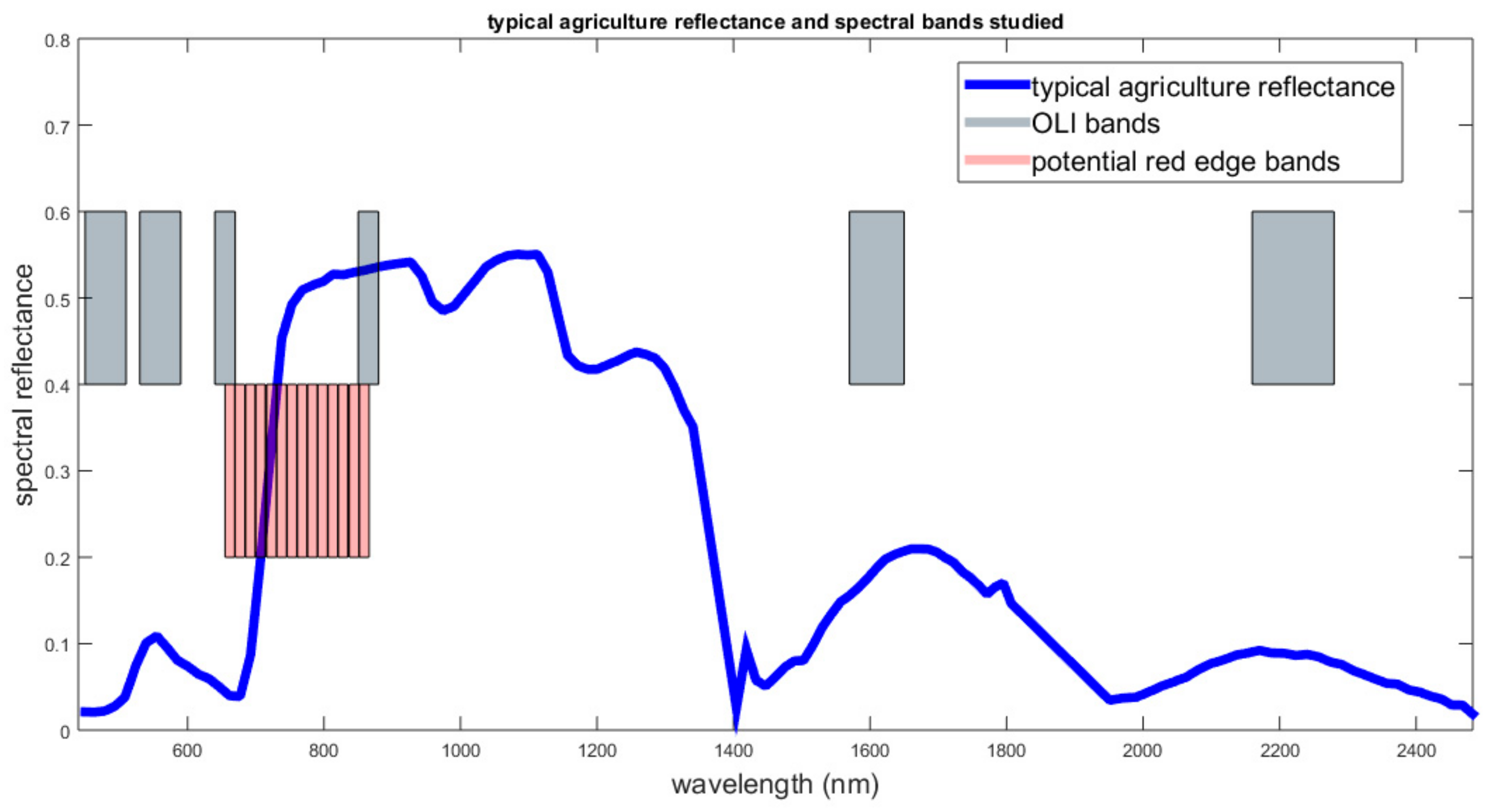
During the campaign, airborne hyperspectral HyMap images and CHRIS/PROBA satellite images were acquired. HyMap provides 125 contiguous spectral bands ranging from 450 nm to 2500 nm. Its average spectral bandwidth is 15–16 nm for visible, NIR and SWIR1 bands and 18–20 nm for SWIR2 bands [27]. CHRIS was configured in Mode 1 and provides 62 spectral bands ranging from 400 nm to 1050 nm. Since our study focused on future Landsat missions that include SWIR bands, we used the HyMap data for our work. The HyMap radiance data were atmospherically compensated to reflectance and georeferenced by DLR [28]. We then spectrally resampled these reflectances to the Landsat 8 OLI surface sensing bands (blue, green, red, NIR, SWIR1, and SWIR2). Finally, all original HyMap bands within OLI red and OLI NIR bands were preserved as potential new spectral band candidates to be considered for future Landsat instruments. Figure 1 plots all spectral bands studied in this paper, along with a typical agriculture spectral reflectance.
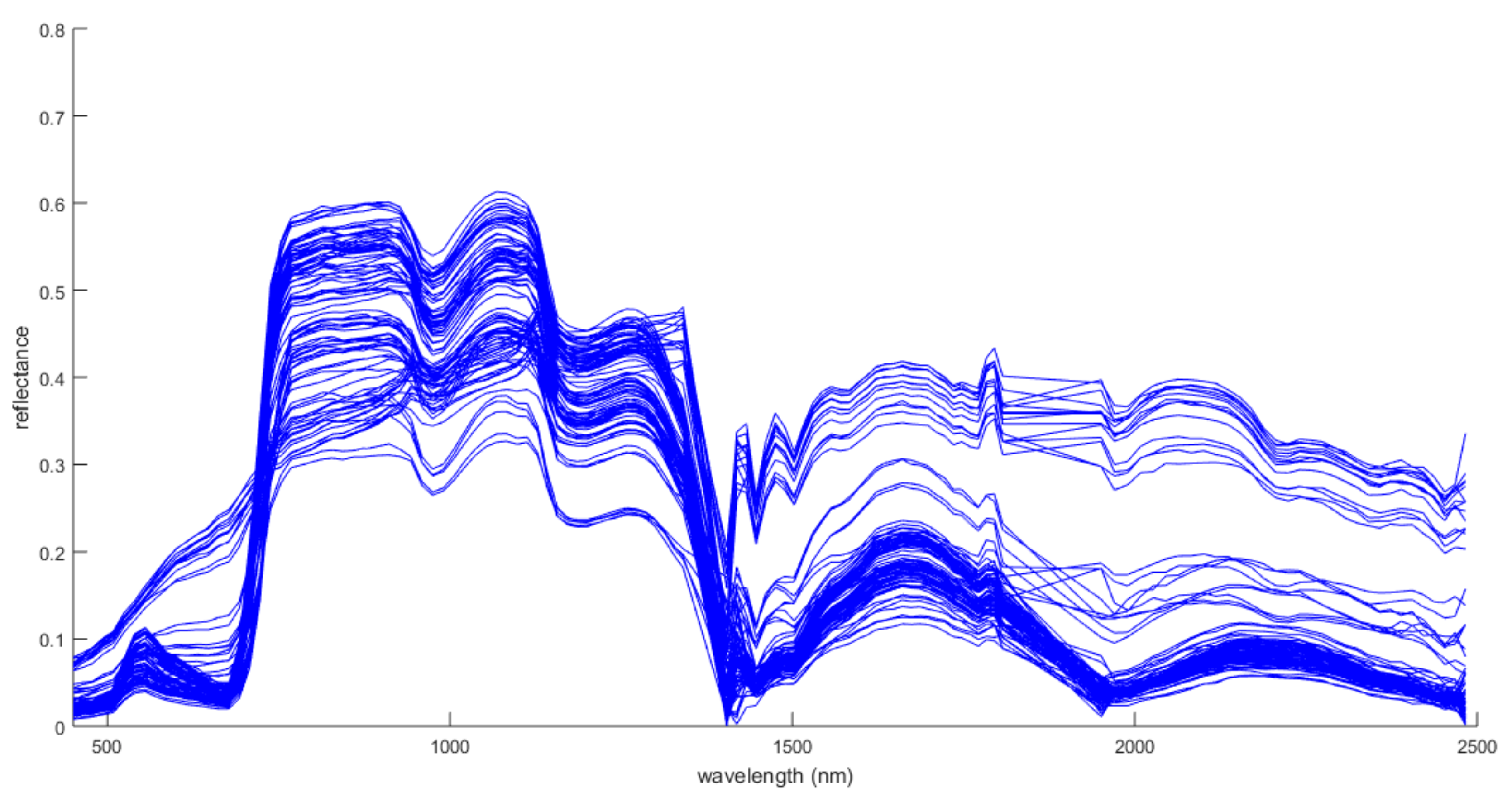
Starting with the 118 ESU samples, we first removed bare soil samples (LAI = 0). Then, brown (dry) LAI samples were also excluded by removing all samples with positive green brown vegetation index (GBVI) values as Equation (1), where and corresponds to spectral reflectance at the band centered at 2000 nm and 2100 nm respectively [28]. In the end, 98 samples were used for this study. Their spectra are shown in Figure 2.
2.2. Methods
2.2.1. Empirical Vegetation Index Approach
Many vegetation indexes have been developed for biophysical parameter estimation. Each has its specific objective and application scope. Among them, the normalized difference vegetation index () is the most widely used due to its simplicity, application to broadband sensors, and compatibility with most operational satellites. The original was developed to highlight the contrast in spectral reflectance between the red and NIR spectral regions, although the combination of red and NIR bands may not be the optimal index to estimate green vegetation LAI. In this study, following the approaches in [24,29,30], all possible -like (normalized difference) spectral band combinations, as shown in (2), were computed and a linear regression between the ground truth LAI and corresponding index value were evaluated.
here and correspond to the spectral reflectances at bands centered at wavelengths a and b. In this study, a five-fold cross-validation scheme was adopted to increase the regression robustness.
2.2.2. Support Vector Regression Approach
Support vector regression (SVR) retrievals were tested to represent a machine learning approach for LAI retrieval. SVR performs linear regression in the high-dimensional feature space spanned from the original spectral reflectance spectra. It has a good compromise between model complexity and prediction power. Previously, SVR has been successfully used for LAI retrieval [14,33]. In this study, the radial basis function (RBF) kernel was used. The RBF kernel can capture the non-linear relationship between input sample dimensions. It has only two free parameters and is easy to tune. During the SVR training process, grid search and cross validation were adopted to estimate the optimal regressor parameters [34].
2.2.3. Look-Up-Table Inversion Approach
Compared to empirical parametric VI approaches or machine learning approaches, the look-up-table (LUT) inversion approach does not require a training dataset to determine the model, which makes it suitable for operational vegetation biophysical variable estimation tasks [5]. The most widely used way to build a LUT is by using RTM simulations. The PROSAIL RTM was used in this study due to its reasonable model assumptions and simplicity. PROSAIL, which is a combination of the leaf optical properties model PROSPECT and the canopy bidirectional reflectance model SAIL, allows a description of both the spectral and directional variation of canopy reflectance as a function of leaf biochemistry and canopy architecture [9]. The PROSAIL model has been validated by comparison to both in situ measurements and other radiative transfer models using benchmark simulated crop canopy structures [35].
4, the leaf model, simulates the bi-Lambertian reflectance and transmittance of leaves as
where is the leaf structure parameter, is the concentration of chlorophyll a and b, is the equivalent water thickness in leaf, and is the leaf dry matter per unit area [9].
4 [36], the canopy model, simulates the bidirectional reflectance factor of turbid medium plant canopies by solving four stream radiative fluxes. The canopy reflectance from the 4SAIL model can be expressed as
where and are leaf reflectance and transmittance spectra from , is the leaf area index, is the average leaf angle, is the hot spot parameter describing the ratio between leaf size and the canopy height, is the soil scaling factor, is the diffuse incoming solar radiation and are the sun zenith angle, view zenith angle, and relative azimuth angle respectively.
In this study, the LUT was generated using MATLAB toolbox ARTMO [37]. The distribution of PROSAIL model input variables were set the same as in [26] as shown in Table 1. The input variable distribution covers most of the ground truth ranges in the SPARC ‘03 campaign. Also, the soil spectrum required by the SAIL model was represented by the mean of all bare soil sample spectra.
To build the LUT, leaf chlorophyll concentration and LAI were randomly sampled 100 times. Each of the other variables were randomly sampled 10 times. All parameter combinations resulted in 1010 simulations. To achieve a compromise between good retrieval accuracy and reasonable processing time, as suggested in [11,38], a random subset of 100,000 sample spectra out of 1010 were selected as LUT entries. These spectra were spectrally resampled with respect to our study bands. Also, as suggested by [26], during the inversion process each SPARC spectra was compared with each sample in the LUT using a Pearson chi-square cost function as shown in (6)
where is the number of bands considered, and corresponds to SPARC sample spectral reflectance and LUT sample spectral reflectance at band n. The first 500 LUT samples with minimum cost function value were identified as candidate solutions. Their mean LAI was selected as the estimated parameter. The means of the first 250, 750, and 1000 solutions were also tested and no significant differences from using 500 samples were observed.
3. Results and Discussion
3.1. Empirical Vegetation Index Approach
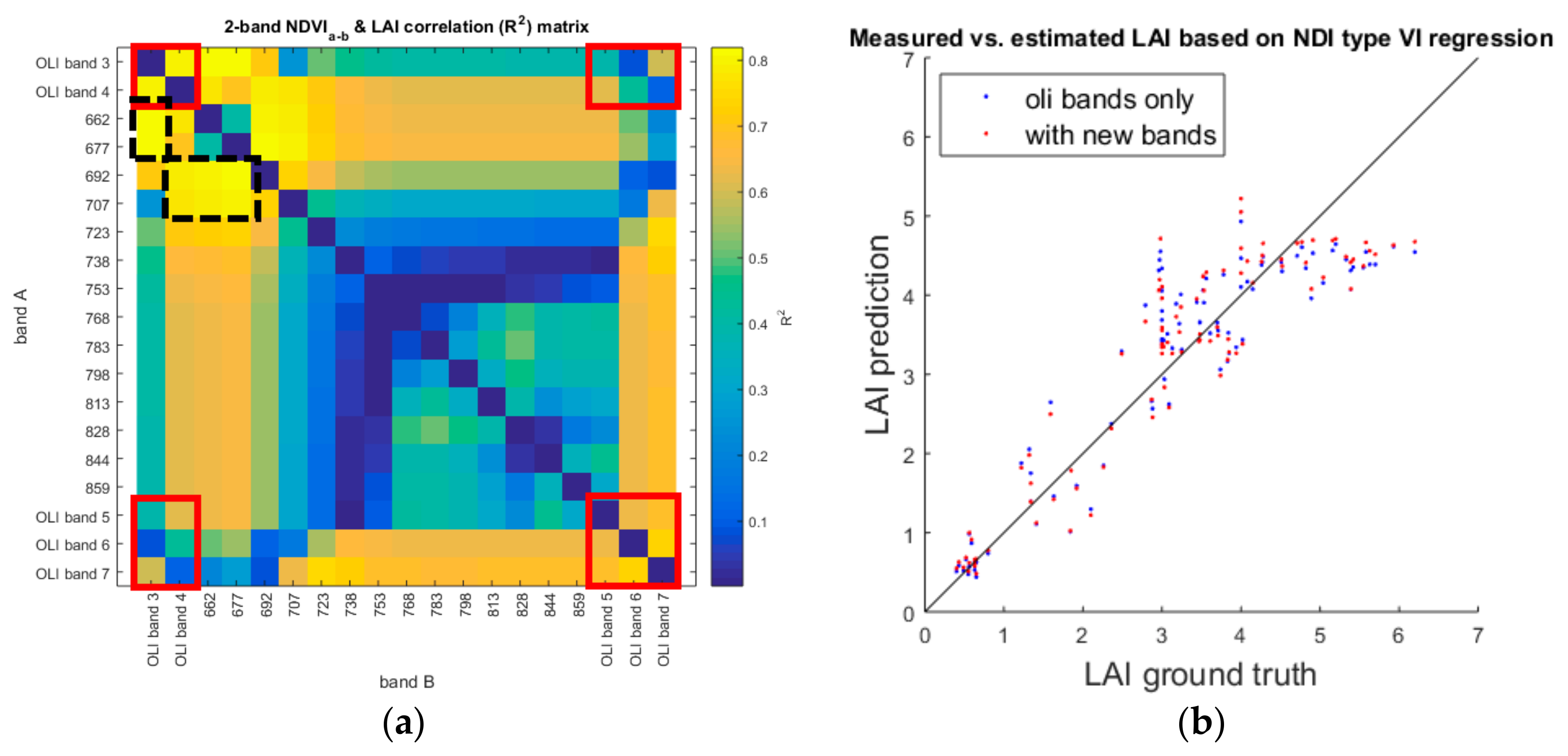
The R2 between ground truth LAI and all possible two-band combination are plotted in Figure 3a. The red box on the corners corresponds to the VIs composed with Landsat 8 OLI bands only. The black dashed boxes highlight the spectral band combinations that gave the highest R2 performance.
The R2 of based on Landsat 8 OLI red and NIR bands () was 0.64 ± 0.05. We observed this was not even the optimal band combination when only OLI bands were considered. The R2 of the combination of OLI SWIR1 and SWIR2 bands was 0.74 ± 0.03. In [26], Verrelst et al. used the same dataset and tested the relationship between all possible Sentinel-2 band combination VIs and LAI. They found the optimal band combination is Sentinel-2 SWIR1 and SWIR2 bands with R2 of 0.739. In our study, though we achieved similar R2 with OLI SWIR1 and SWIR2 bands, we achieved higher R2 performance with the combination of OLI green and red bands. One explanation for this could be the difference of red band central wavelengths between Sentinel-2 and Landsat 8 OLI. A small wavelength difference in this sensitive spectral range can cause differences in product retrieval performance.
When potential new bands were considered, two R2 peaks were observed in Figure 3a. One peak is in the spectral range of 655–677 nm and 692–707 nm. The optimal band combination in this peak is 677 nm and 707 nm, with an R2 of 0.79 ± 0.07. This is very similar to the observation in [24] using the same field campaign data where the optimal band combination for LAI retrieval was found as 674 nm and 712 nm. The difference is that in [24] the authors used high spectral resolution CHRIS data instead of the HyMap data used in this study and they could study the optimal band combination at a higher spectral resolution. However, they only tested the spectral range between 600 nm and 1000 nm in [24]. In our study, beyond the spectral range studied in [24], a second R2 peak were found near the green band region containing the overall best performance band combination. The combination of OLI green and 677 nm or 662 nm band resulted in LAI estimation with an R2 of 0.81 ± 0.07, which is slightly higher than the combination of OLI red and green. This suggests that for agroecosystems, a new spectral band centered near 662–677 nm will slightly improve the performance of based LAI estimation by a few percent. Figure 3b shows the scatter plot of LAI estimation based on . Blue scatter corresponds to the OLI optimal band combination (bands green and red) and red scatter corresponds to the optimal band combination when all potential new bands were considered (bands green and 677 nm). Two observations can be made: (1) the two sets of band combinations perform very similar; and (2) as reported in previous studies [17,26], the VI based approach suffers from a saturation effect, which can cause underestimation of high LAI (>5) values.
Similarly, the results of all band combinations for are plotted in Figure 4a. When considering OLI bands only, the optimal band combination is OLI green and red bands with an R2 of 0.77 ± 0.03. When all potential new bands are considered, similar to the result, a peak is observed in the 655–677 nm and 692–707 nm regions. The optimal band combination was found to be 692 nm and 677 nm with an R2 = 0.81 ± 0.05. The scatter plot of optimal band combination based LAI estimation is shown in Figure 4b. In general, the result was very similar to the results in that a slight improvement in agroecosystem green LAI estimation is predicted from the addition of a new spectral band between the OLI red and NIR bands in future Landsat instruments.
3.2. LUT Inversion Result
Compared to regression-based approaches which requires calibration data to calibrate the regression model, LUT inversion is more practical for operational level LAI estimation. In this study, first, all possible OLI band combinations ( 63 cases) were tested for LUT inversion. Then the band settings involving potential new band(s) were tested. Up to 3 out of 14 new potential bands were considered. The total number of cases of the addition of 0, 1, 2, or 3 new potential bands are listed in Table 2.
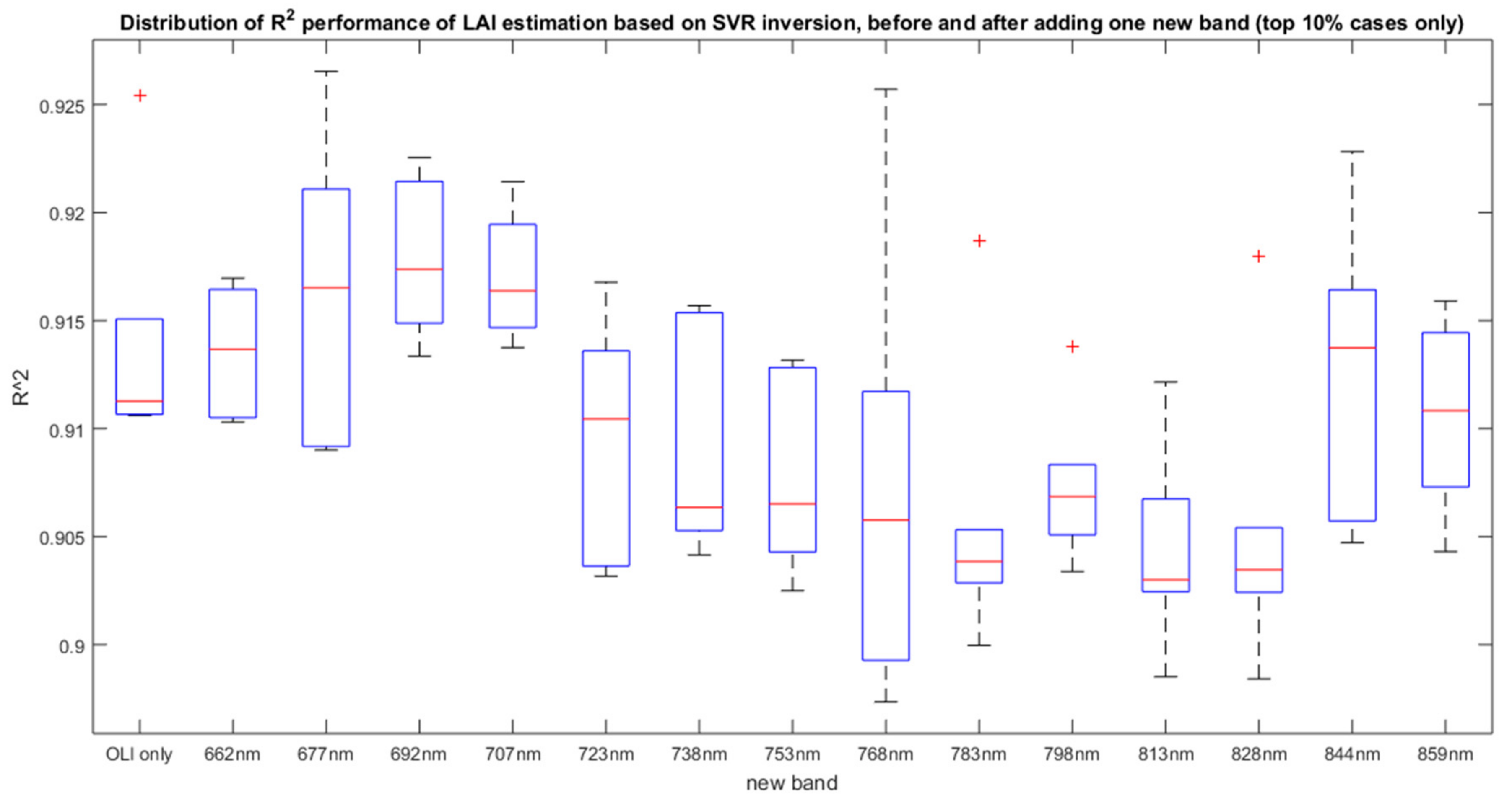
Figure 5 is a summary of the LUT inversion results of using no new bands or the addition of one new potential band. The leftmost result corresponds to the statistics of top 10% performing OLI band only combinations, which serve as a baseline. In all cases, each blue box corresponds to the range of the top 10% band combinations when each new potential band was added. For example, the 662 nm box corresponds to the top 10% of the combinations that 662 nm band together with all possible 64 OLI band combinations. In each box, the red line is the average performance and the lower and upper boundaries of the box are the first and third quartile performance. The red crosses correspond to outliers.
For the combination using OLI bands only, the optimal band combination is green/red/NIR/SWIR1/SWIR2 with an R2 of 0.806. If we consider the best performing cases for each new potential band added, two spectral range peaks can be observed: 662–677 nm and 723–738 nm. The overall best performance is 662 nm/OLI band 3 (green)/NIR/SWIR1/SWIR2 with R2 of 0.828.
The statistics of R2 of the top 10% cases of adding no (0), 1, 2, or 3 new potential bands were examined and are shown in Figure 6. Due to the enormous number of band combinations, the details of adding two or three new bands are not listed in this paper. We observed that the addition of two or three new bands only slightly improved the LAI estimation performance (less than 0.01 in R2), compared to adding one new band.
3.3. Support Vector Regression Result
Figure 7 is a summary of studying zero or one new potential band using the SVR approach. The interpretation is similar to the result of LUT inversion shown in Figure 5. The R2 of the cases in Figure 7 are in a small range from 0.90 to 0.925. The overall performance was higher than the VI and LUT inversion approaches, which is reasonable because of the power of non-linear regression. However, the limited variation range (less than 0.03) indicates the SVR result may have suffered from over fitting. If we consider the best case for each new band added, almost no improvement was achieved after adding any of these potential new bands. If we consider the average performance of each column, the new bands within the spectral range between 677 nm and 707 nm were seen to improve the LAI retrieval accuracy, although the advantage was minimal. The retrieval results of the addition of two or three new bands are not listed here because no significant improvement was observed.
3.4. Discussion
Table 3 summarizes the LAI estimation performance before and after the addition of potential new spectral bands using the three approaches studied. For each approach, the optimal new band spectral range is listed as well.
All three approaches show a small improvement from the addition of new potential bands. This is not too surprising and has been seen in previous studies, both in simulated and real data. For the estimation of agroecosystem green LAI, using the same SPARC ‘03 field campaign data, ref [13] studied different machine learning algorithms for biophysical parameter retrieval based on simulated Sentinel-2 imagery. They found limited improvement in Gaussian process regression (GPR) based LAI estimation after including Sentinel-2 red edge bands (R2 = 0.91), compared to using just the Sentinel-2 blue, green, red, and NIR bands (R2 = 0.910). Also, the GPR significance analysis showed that the red edge bands are less important than Sentinel-2 blue, green, and NIR bands. Researchers in [24] used SPARC ‘03 and ‘04 CHRIS data to search for optimal two-band combinations for LAI estimation based on a VI approach. The R2 of their optimal band settings (674 nm and 712 nm) was 0.824, which was only a slight increase from the combination of OLI red and NIR (R2 ~ 0.78). Researchers in [18] studied the LAI estimation in both LUT inversion and artificial neural network approaches with Sentinel-2 band settings. They studied the significance of each Sentinel-2 spectral band by counting the frequency each band appeared in the top 5% band combinations. In their result, the three Sentinel-2 red edge bands did not show dominance over the other spectral bands. For single species crop biophysical parameters retrieval, [21] used real Sentinel-2 data to study the VI approach based potato crop LAI and canopy chlorophyll content (CCC) estimation. They concluded that Sentinel-2 10 m bands (blue, green, red, NIR) are better than 20 m bands (red edge bands) for LAI and CCC retrieval. While not a study using agriculture crops, [22] compared the LAI estimation performance of boreal forest canopy while using real Sentinel-2 and Landsat-8 data. Their results using Sentinel-2 data were slightly better than the result based on Landsat-8 OLI data (R2 = 0.734 vs. R2 = 0.725), even though Sentinel-2 has three red edge bands and Landsat-8 OLI does not have one. Researchers in [29] estimated LAI of a cotton canopy through a VI approach. After going through all possible band combinations, they observed a 2.2% improvement in R2 using their optimal band combination (700 and 800 nm) over the combination of Landsat TM red and NIR bands.
Considering Table 3, both VI and LUT approaches have two optimal new band spectral ranges. The common range is 662–677 nm. This is not surprising and two possible reasons can explain this. First, the correlation coefficients between the ground truth LAI and spectral reflectance reach a maximum absolute value near 662–677 nm. As suggested in [39], it is beneficial to select an instrument spectral band centered at wavelengths with high correlation coefficients. Second, the bandpass of the OLI red band is from 636 nm to 673 nm, which is wide compared to the studied HyMap bandwidth (~15 nm in VIS and NIR). The bandpass of HyMap 662 nm is approximately from 655 nm to 670 nm. This is entirely within the OLI red bandpass. In this wavelength range that is very sensitive to biophysical parameter changes, the narrower HyMap 662 nm band may better capture the spectral reflectance subtle difference caused by LAI difference than the existing OLI red band. This was verified in our results by the observation that in the top performing band combinations in the LUT inversion approach the narrow 662 nm band was selected more often than the existing OLI red band.
Our results have some differences with previous studies that focused on canopy LAI retrieval for a single crop species. In our work, the small improvement observed from the addition of new bands may be due in part to the fact we considered a complex agroecosystem of nine crop species at different growth stages. This may have overwhelmed the spectral features located in the red edge region for a single crop species. However, our results are representative of typical application of operational methods and demonstrate anticipated performance gains across a wide range of vegetation crop types and growth stages.
4. Summary
In this paper, the potential of adding new spectral bands in future Landsat instruments for agroecosystem green LAI retrieval was studied. Three categories of retrieval approaches were tested: empirical vegetation index regression ( and ), physical based LUT inversion, and machine learning (SVR). The results from all three approaches suggested that a limited retrieval accuracy increase can be achieved after the addition of at most three new spectral bands located between the OLI red and NIR bands. In both the VI and LUT approaches, a new band centered in the range from 662 nm to 677 nm was observed to provide a small improvement in performance. However, this result may be due to the fact that the new bands studied were narrower than the current OLI red band and closer to the wavelength most sensitive to LAI change. In general, the addition of new red edge bands in future Landsat instruments may be of only marginal benefit to agroecosystem green LAI retrieval. This is consistent with conclusions from previous studies that the three Sentinel-2 red-edge bands may not have been significantly beneficial for agriculture green LAI retrieval.
Author Contributions
Z.C. conceived of, designed, and carried out the experiments and wrote the majority of the paper. J.P.K. provided guidance during the work and contributed to the writing and editing of the paper.
Funding
This work has been supported in part by the National Aeronautics and Space Administration under grant number NNX14AP40G.
Acknowledgments
The authors thank Jochem Verrelst for sharing the SPARC ‘03 data.
Conflicts of Interest
The authors declare no conflict of interest.
References
- Myneni, R.B.; Hoffman, S.; Knyazikhin, Y.; Privette, J.L.; Glassy, J.; Tian, Y.; Wang, Y.; Song, X.; Zhang, Y.; Smith, G.R.; et al. Global products of vegetation leaf area and fraction absorbed PAR from year one of MODIS data. Remote Sens. Environ. 2002, 83, 214–231. [Google Scholar] [CrossRef] [Green Version]
- Bacour, C.; Baret, F.; Béal, D.; Weiss, M.; Pavageau, K. Neural network estimation of LAI, fAPAR, fCover and LAI× Cab, from top of canopy MERIS reflectance data: Principles and validation. Remote Sens. Environ. 2006, 105, 313–325. [Google Scholar] [CrossRef]
- Horler, D.N.; Dockray, M.; Barber, J. The red edge of plant leaf reflectance. Int. J. Remote Sens. 1983, 4, 273–288. [Google Scholar] [CrossRef]
- Ganguly, S.; Nemani, R.R.; Zhang, G.; Hashimoto, H.; Milesi, C.; Michaelis, A.; Wang, W.; Votava, P.; Samanta, A.; Melton, F.; et al. Generating global leaf area index from Landsat: Algorithm formulation and demonstration. Remote Sens. Environ. 2012, 122, 185–202. [Google Scholar] [CrossRef]
- Baret, F.; Buis, S. Estimating canopy characteristics from remote sensing observations: Review of methods and associated problems. In Advances in Land Remote Sensing; Springer: Dordrecht, The Netherlands, 2008; pp. 173–201. [Google Scholar]
- Verrelst, J.; Camps-Valls, G.; Muñoz-Marí, J.; Rivera, J.P.; Veroustraete, F.; Clevers, J.G.; Moreno, J. Optical remote sensing and the retrieval of terrestrial vegetation bio-geophysical properties: A review. ISPRS J. Photogramm. Remote Sens. 2015, 108, 273–290. [Google Scholar] [CrossRef]
- Delegido, J.; Verrelst, J.; Alonso, L.; Moreno, J. Evaluation of sentinel-2 red-edge bands for empirical estimation of green LAI and chlorophyll content. Sensors 2011, 11, 7063–7081. [Google Scholar] [CrossRef] [PubMed]
- Wu, C.; Wang, L.; Niu, Z.; Gao, S.; Wu, M. Nondestructive estimation of canopy chlorophyll content using Hyperion and Landsat/TM images. Int. J. Remote Sens. 2010, 31, 2159–2167. [Google Scholar] [CrossRef]
- Jacquemoud, S.; Verhoef, W.; Baret, F.; Bacour, C.; Zarco-Tejada, P.J.; Asner, G.P.; François, C.; Ustin, S.L. PROSPECT + SAIL models: A review of use for vegetation characterization. Remote Sens. Environ. 2009, 113, 56–66. [Google Scholar] [CrossRef]
- Richter, K.; Atzberger, C.; Vuolo, F.; D’Urso, G. Evaluation of sentinel-2 spectral sampling for radiative transfer model based LAI estimation of wheat, sugar beet, and maize. IEEE J. Sel. Top. Appl. Earth Obs. Remote Sens. 2011, 4, 458–464. [Google Scholar] [CrossRef]
- Darvishzadeh, R.; Matkan, A.A.; Ahangar, A.D. Inversion of a radiative transfer model for estimation of rice canopy chlorophyll content using a lookup-table approach. IEEE J. Sel. Top. Appl. Earth Obs. Remote Sens. 2012, 5, 1222–1230. [Google Scholar] [CrossRef]
- Duan, S.B.; Li, Z.L.; Wu, H.; Tang, B.H.; Ma, L.; Zhao, E.; Li, C. Inversion of the PROSAIL model to estimate leaf area index of maize, potato, and sunflower fields from unmanned aerial vehicle hyperspectral data. Int. J. Appl. Earth Obs. Geoinf. 2014, 26, 12–20. [Google Scholar] [CrossRef]
- Verrelst, J.; Muñoz, J.; Alonso, L.; Delegido, J.; Rivera, J.P.; Camps-Valls, G.; Moreno, J. Machine learning regression algorithms for biophysical parameter retrieval: Opportunities for Sentinel-2 and-3. Remote Sens. Environ. 2012, 118, 127–139. [Google Scholar] [CrossRef]
- Vuolo, F.; Neugebauer, N.; Bolognesi, S.F.; Atzberger, C.; D’Urso, G. Estimation of leaf area index using DEIMOS-1 data: Application and transferability of a semi-empirical relationship between two agricultural areas. Remote Sens. 2013, 5, 1274–1291. [Google Scholar] [CrossRef]
- Fang, H.; Liang, S.; Kuusk, A. Retrieving leaf area index using a genetic algorithm with a canopy radiative transfer model. Remote Sens. Environ. 2003, 85, 257–270. [Google Scholar] [CrossRef]
- Walthall, C.; Dulaney, W.; Anderson, M.; Norman, J.; Fang, H.; Liang, S. A comparison of empirical and neural network approaches for estimating corn and soybean leaf area index from Landsat ETM+ imagery. Remote Sens. Environ. 2004, 92, 465–474. [Google Scholar] [CrossRef]
- González-Sanpedro, M.C.; Le Toan, T.; Moreno, J.; Kergoat, L.; Rubio, E. Seasonal variations of leaf area index of agricultural fields retrieved from Landsat data. Remote Sens. Environ. 2008, 112, 810–824. [Google Scholar] [CrossRef]
- Richter, K.; Hank, T.B.; Vuolo, F.; Mauser, W.; D’Urso, G. Optimal exploitation of the Sentinel-2 spectral capabilities for crop leaf area index mapping. Remote Sens. 2012, 4, 561–582. [Google Scholar] [CrossRef] [Green Version]
- Herrmann, I.; Pimstein, A.; Karnieli, A.; Cohen, Y.; Alchanatis, V.; Bonfil, D.J. LAI assessment of wheat and potato crops by VENμS and Sentinel-2 bands. Remote Sens. Environ. 2011, 115, 2141–2151. [Google Scholar] [CrossRef]
- Fernandes, R.; Weiss, M.; Camacho, F.; Berthelot, B.; Baret, F.; Duca, R. Development and assessment of leaf area index algorithms for the Sentinel-2 multispectral imager. In Proceedings of the Geoscience and Remote Sensing Symposium (IGARSS), Quebec City, QC, Canada, 13–18 July 2014; pp. 3922–3925. [Google Scholar]
- Clevers, J.; Kooistra, L.; Van Den Brande, M. Using Sentinel-2 data for retrieving LAI and leaf and canopy chlorophyll content of a potato crop. Remote Sens. 2017, 9, 405. [Google Scholar] [CrossRef]
- Korhonen, L.; Packalen, P.; Rautiainen, M. Comparison of Sentinel-2 and Landsat 8 in the estimation of boreal forest canopy cover and leaf area index. Remote Sens. Environ. 2017, 195, 259–274. [Google Scholar] [CrossRef]
- Rengarajan, R. Evaluation of Sensor, Environment and Operational Factors Impacting the Use of Multiple Sensor Constellations for Long Term Resource Monitoring. Ph.D. Thesis, Rochester Institute of Technology, Rochester, NY, USA, 2016. [Google Scholar]
- Delegido, J.; Verrelst, J.; Meza, C.M.; Rivera, J.P.; Alonso, L.; Moreno, J. A red-edge spectral index for remote sensing estimation of green LAI over agroecosystems. Eur. J. Agron. 2013, 46, 42–52. [Google Scholar] [CrossRef]
- Moreno, J.F.; Alonso, L.; Fernández, G.; Fortea, J.C.; Gandía, S.; Guanter, L.; García, J.C.; Martí, J.M.; Melia, J.; De Coca, F.C.; et al. The SPECTRA Barrax Campaign (SPARC): Overview and first results from CHRIS data. Eur. Space Agency Spec. Publ. SP 2004, 578, 30–39. [Google Scholar]
- Verrelst, J.; Rivera, J.P.; Veroustraete, F.; Muñoz-Marí, J.; Clevers, J.G.; Camps-Valls, G.; Moreno, J. Experimental Sentinel-2 LAI estimation using parametric, non-parametric and physical retrieval methods: A comparison. ISPRS J. Photogramm. Remote Sens. 2015, 108, 260–272. [Google Scholar] [CrossRef]
- Cocks, T.; Jenssen, R.; Stewart, A.; Wilson, I.; Shields, T. The HyMapTM airborne hyperspectral sensor: The system, calibration and performance. In Proceedings of the 1st EARSEL Workshop on Imaging Spectroscopy, Zurich, Switzerland, 6 October 1998. [Google Scholar]
- Delegido Jesús, J.; Verrelst, J.; Rivera, J.P.; Ruiz-Verdú, A.; Moreno, J. Brown and green LAI mapping through spectral indices. Int. J. Appl. Earth Obs. Geoinf. 2015, 35, 350–358. [Google Scholar] [CrossRef]
- Zhao, D.; Huang, L.; Li, J.; Qi, J. A comparative analysis of broadband and narrowband derived vegetation indices in predicting LAI and CCD of a cotton canopy. ISPRS J. Photogramm. Remote Sens. 2007, 62, 25–33. [Google Scholar] [CrossRef]
- Darvishzadeh, R.; Atzberger, C.; Skidmore, A.; Schlerf, M. Mapping grassland leaf area index with airborne hyperspectral imagery: A comparison study of statistical approaches and inversion of radiative transfer models. ISPRS J. Photogramm. Remote Sens. 2011, 66, 894–906. [Google Scholar] [CrossRef]
- Gitelson, A.A.; Vina, A.; Ciganda, V.; Rundquist, D.C.; Arkebauer, T.J. Remote estimation of canopy chlorophyll content in crops. Geophys. Res. Lett. 2005, 32, L08403.1–L08403.4. [Google Scholar] [CrossRef]
- Clevers, J.G.; Gitelson, A.A. Remote estimation of crop and grass chlorophyll and nitrogen content using red-edge bands on Sentinel-2 and-3. Int. J. Appl. Earth Obs. Geoinf. 2013, 23, 344–351. [Google Scholar] [CrossRef]
- Durbha, S.S.; King, R.L.; Younan, N.H. Support vector machines regression for retrieval of leaf area index from multiangle imaging spectroradiometer. Remote Sens. Environ. 2007, 107, 348–361. [Google Scholar] [CrossRef]
- Hsu, C.W.; Chang, C.C.; Lin, C.J. A Practical Guide to Support Vector Classification; Department of Computer Science and Information Engineering, National Taiwan University: Taipei, Taiwan, 2003. [Google Scholar]
- European Commission. RAMI. Available online: http://rami-benchmark.jrc.ec.europa.eu/HTML/RAMI3/RAMI3.php (accessed on 20 May 2017).
- Verhoef, W.; Bach, H. Coupled soil–leaf-canopy and atmosphere radiative transfer modeling to simulate hyperspectral multi-angular surface reflectance and TOA radiance data. Remote Sens. Environ. 2007, 109, 166–182. [Google Scholar] [CrossRef]
- Verrelst, J.; Romijn, E.; Kooistra, L. Mapping vegetation structure in a heterogeneous river floodplain ecosystem using pointable CHRIS/PROBA data. Remote Sens. 2012, 4, 2866–2889. [Google Scholar] [CrossRef]
- Weiss, M.; Baret, F.; Myneni, R.; Pragnère, A.; Knyazikhin, Y. Investigation of a model inversion technique to estimate canopy biophysical variables from spectral and directional reflectance data. Agronomie 2000, 20, 3–22. [Google Scholar] [CrossRef]
- Frampton, W.J.; Dash, J.; Watmough, G.; Milton, E.J. Evaluating the capabilities of Sentinel-2 for quantitative estimation of biophysical variables in vegetation. ISPRS J. Photogramm. Remote Sens. 2013, 82, 83–92. [Google Scholar] [CrossRef]
Figure 1.
Spectral bands studied in this work (OLI bands and potential red edge bands) and typical agriculture spectral reflectance.
Figure 1.
Spectral bands studied in this work (OLI bands and potential red edge bands) and typical agriculture spectral reflectance.

Figure 2.
The 98 SPARC ‘03 campaign HyMap spectra used in our study.

Figure 3.
(a) R2 between ground truth LAI and for different band combinations; (b) Scatter plot of the predicted LAI versus ground truth LAI. Blue is from the , red is from
Figure 3.
(a) R2 between ground truth LAI and for different band combinations; (b) Scatter plot of the predicted LAI versus ground truth LAI. Blue is from the , red is from

Figure 4.
(a) R2 between ground truth LAI and for different band combinations. (b) Scatter plot of the predicted LAI versus ground truth LAI. Blue is from the , red is from .
Figure 4.
(a) R2 between ground truth LAI and for different band combinations. (b) Scatter plot of the predicted LAI versus ground truth LAI. Blue is from the , red is from .
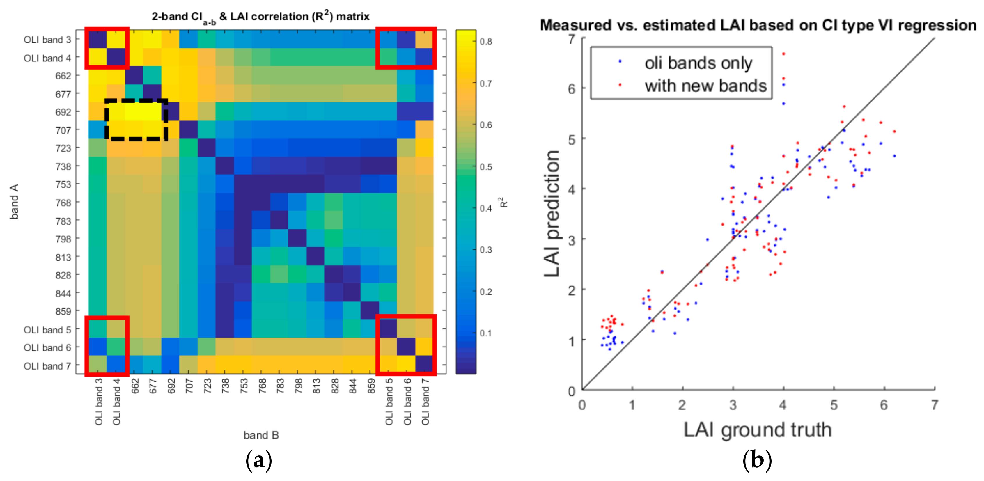
Figure 5.
Statistics of top 10% performance of adding 0/1 new bands in LUT inversion approach.
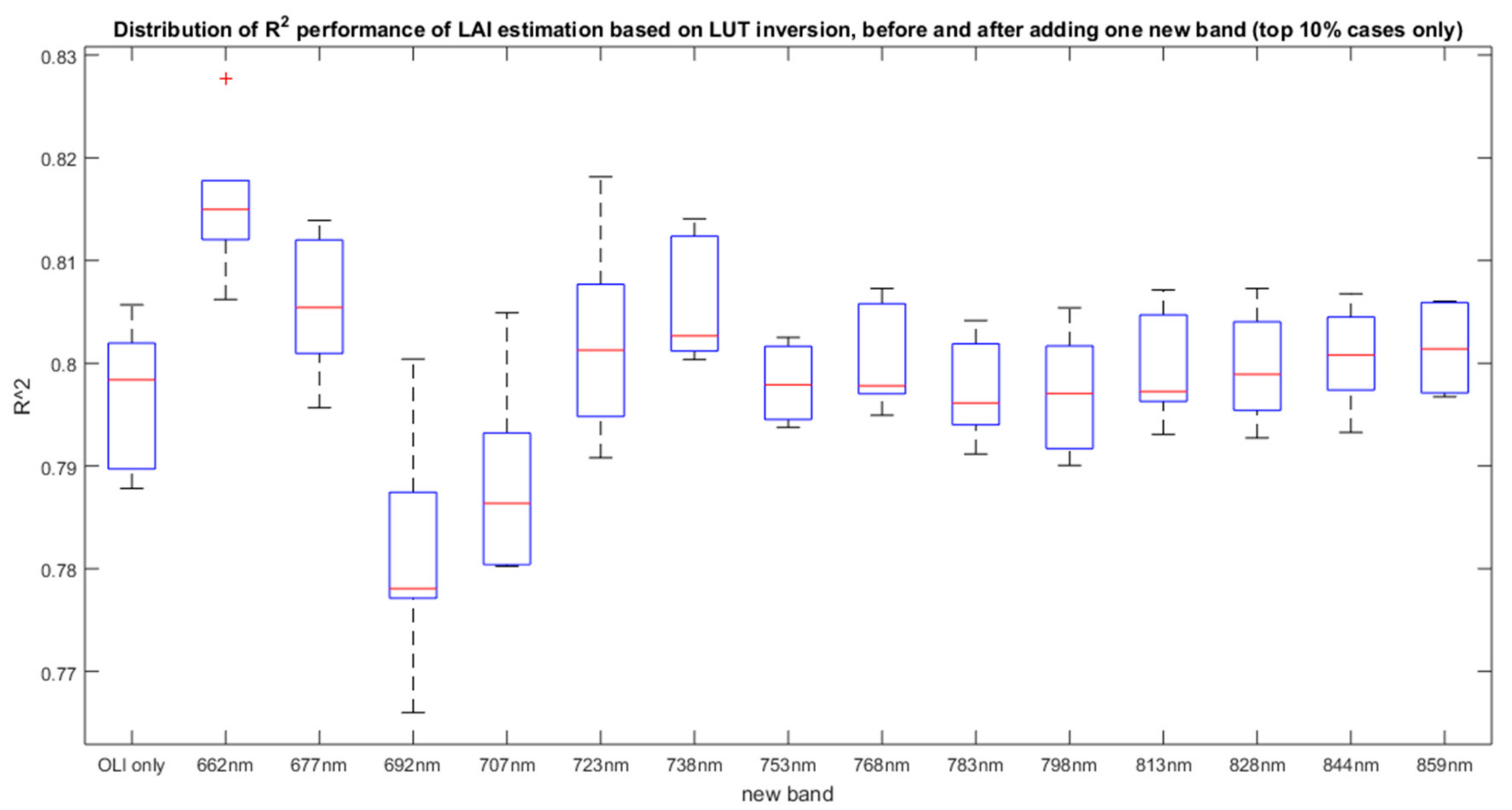
Figure 6.
Statistics of top 10% performing cases of adding 0/1/2/3 new bands in LUT inversion approach.
Figure 6.
Statistics of top 10% performing cases of adding 0/1/2/3 new bands in LUT inversion approach.
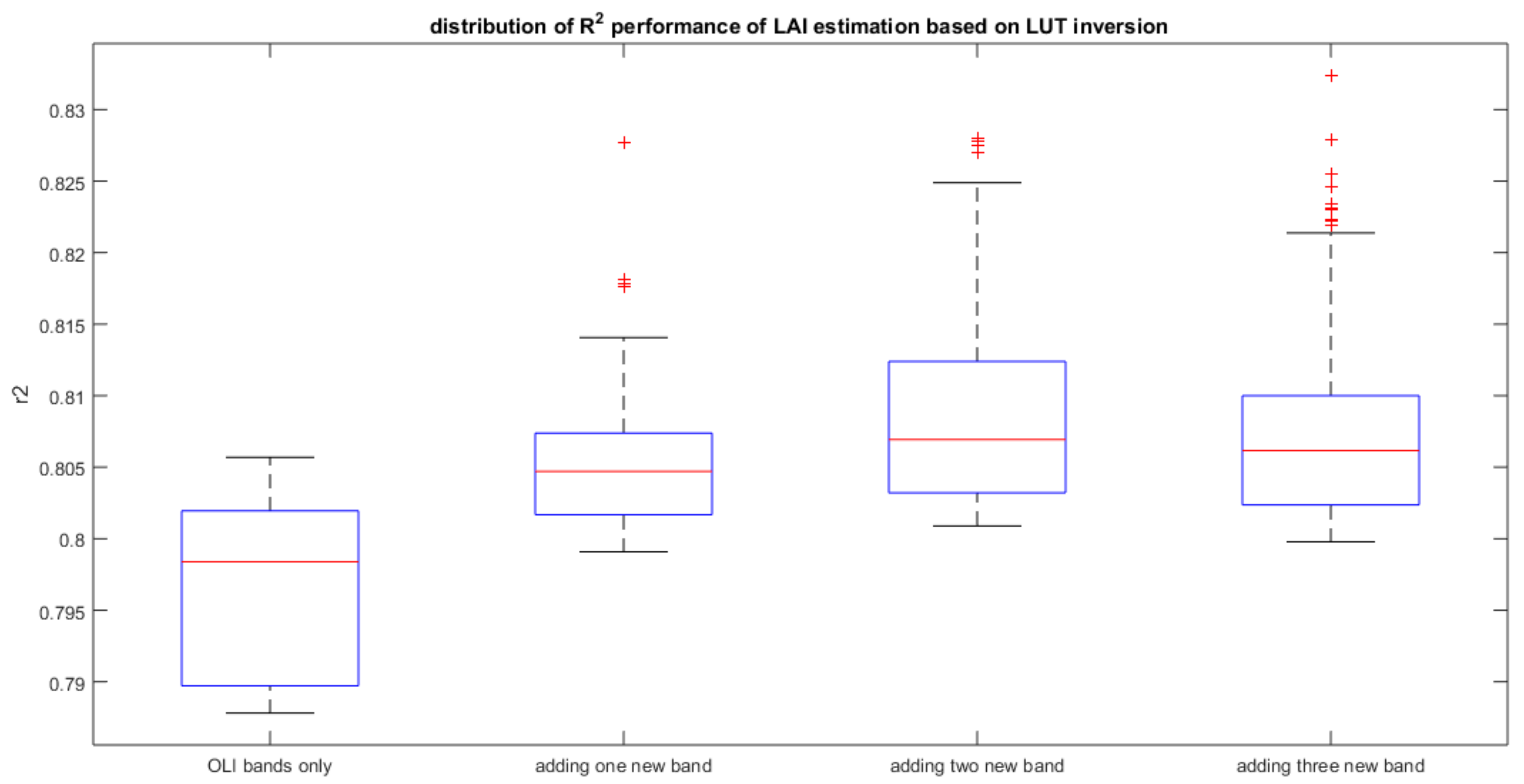
Figure 7.
Statistics of top 10% performance of adding 0/1 new bands in SVR approach.


Table 1.
Range and distribution of input parameters used to drive PROSAIL model to generate LUT.
| Model Parameters | Units | Range | Distribution | |
|---|---|---|---|---|
| Leaf parameters: PROSPECT-4 | ||||
| N | Leaf structure index | Unitless | 1.3–2.5 | Uniform |
| Leaf chlorophyll content | 5–75 | ) | ||
| Leaf dry matter content | 0.001–0.03 | Uniform | ||
| Leaf water content | 0.002–0.05 | Uniform | ||
| Canopy variables: 4SAIL | ||||
| Leaf area index | 0.1–7 | ) | ||
| Soil scaling factor | Unitless | 0–1 | Uniform | |
| Average leaf angle | Degree | 40–70 | Uniform | |
| Hot spot parameter | 0.05–0.5 | Uniform | ||
| Diffuse incoming solar radiation | (fraction) | 0.05 | - | |
| Sun zenith angle | Degree | 22.3 | - | |
| View zenith angle | Degree | 0 | - | |
| Sun-sensor azimuth angle | Degree | 0 | - | |
Table 2.
Number of possible band combinations for adding 0/1/2/3 new potential bands.
| OLI Band Cases | New Potential Band Cases | Total Cases | |
|---|---|---|---|
| OLI only | 63 | N/A | 63 |
| One new band | 64 | ) | 896 |
| Two new bands | 64 | ) | 5824 |
| Three new bands | 64 | ) | 23,296 |
Table 3.
Performance and optimal new band center position range of three retrieval approaches.
| LUT (One New Band Only) | SVR | |||||
|---|---|---|---|---|---|---|
| R2 | Optimal two bands center range | R2 | Optimal new band center range | R2 | Optimal new band center range | |
| OLI bands only | 0.787 | OLI band 3 and OLI band 4 | 0.806 | N/A | 0.925 | N/A |
| With new bands | 0.810 | 670 ± 8 nm and 700 ± 8 nm | 0.828 | 670 ± 8 nm or 730 ± 8 nm | 0.933 | 692 ± 15 nm |
© 2018 by the authors. Licensee MDPI, Basel, Switzerland. This article is an open access article distributed under the terms and conditions of the Creative Commons Attribution (CC BY) license (http://creativecommons.org/licenses/by/4.0/).
Share and Cite
MDPI and ACS Style
Cui, Z.; Kerekes, J.P. Potential of Red Edge Spectral Bands in Future Landsat Satellites on Agroecosystem Canopy Green Leaf Area Index Retrieval. Remote Sens. 2018, 10, 1458. https://doi.org/10.3390/rs10091458
AMA Style
Cui Z, Kerekes JP. Potential of Red Edge Spectral Bands in Future Landsat Satellites on Agroecosystem Canopy Green Leaf Area Index Retrieval. Remote Sensing. 2018; 10(9):1458. https://doi.org/10.3390/rs10091458
Chicago/Turabian StyleCui, Zhaoyu, and John P. Kerekes. 2018. "Potential of Red Edge Spectral Bands in Future Landsat Satellites on Agroecosystem Canopy Green Leaf Area Index Retrieval" Remote Sensing 10, no. 9: 1458. https://doi.org/10.3390/rs10091458
Note that from the first issue of 2016, this journal uses article numbers instead of page numbers. See further details here.