A Prediction Smooth Method for Blending Landsat and Moderate Resolution Imagine Spectroradiometer Images

Abstract
:1. Introduction
2. Methodology
2.1. Problem Description
2.2. Modelling of Gradual Vegetation Phenological Changes
2.3. Modelling of Land-Cover Type Changes
- Use the residuals to identify spatial pattern changes within a cluster, then reclassify the pixels within the cluster based on the residual pattern for a new prediction. For instance, if some of the pixels are spatially located together within a cluster have different residuals from others, we may split the pixels of this cluster into two new clusters based on the residual values. One is for the pixels without land-cover change and another is for the pixels with land-cover change, or
- Distribute the residuals to Landsat pixels within the MODIS pixel through an adjustment of the residuals similar to the TPS interpolation used by FSDAF.
2.4. Optimization of Models
- Conduct predictions for a predetermined cluster number range from and calculate their corresponding correlation coefficients between the differences of the Landsat image at t0 and the predicted Landsat-like image at t1 and the differences of the MODIS images at t0 and t1 and sums of the residual squares for all predicted Landsat-like images, respectively;
- Compare the correlation coefficients and the sums of residual squares and select the prediction that meets the MCSR rule as the optimized prediction.
2.5. Smoothing of Forward and Backward Predictions
- Calculate indices (NDSI for snow onset and snowmelt season or NDVI for vegetation growing season) of the input Landsat images at t0 and t2 and the MODIS observation at t1, namely and for forward prediction, backward prediction and the MODIS, respectively. NDSI and NDVI are used separately. When there is snow cover present on at least one image, NDSI is used. NDVI is used for those images in vegetation growing season.
- Check if there are any invalid pixel values in the forward and backward predictions. If one of them is invalid, select the valid pixel as the final pixel;
- Set up an index boundary I0. For example, the boundary I0 is set to 0.4 for snow cover (≥0.4) and snow free (<0.4) situation as it is the commonly used threshold. And then compare the boundary value to the index value , and to determine the final pixel as follows:
- If , select the forward prediction;
- If , select the forward prediction;
- If , select the backward prediction;
- If , select the backward prediction;
- For all other cases, apply weighted average based on the estimated uncertainties or their time intervals between the observation dates and the prediction date.
2.6. Implementation
- Perform forward predictions for predetermined cluster number range from 4 to 16 and determine the optimized forward prediction. This process includes:
- classify the Landsat image at t0 for a specified cluster number;
- calculate the MODIS reflectance change velocity using the MODIS observations at t0 and t1;
- estimate the reflectance change velocity;
- predict Landsat-like image at t1 using the reflectance change velocity of all clusters estimated in step c;
- calculate the correlation coefficient between the differences of the predicted Landsat-like image and Landsat image at t0 and the MODIS image differences;
- calculate residuals of the predicted Landsat-like image and their sum of squares;
- adjust residuals by interpolating them to each Landsat-like image pixels to obtain a new Landsat-like image prediction;
- calculate the correlation coefficient between the differences of the newly predicted Landsat-like image and Landsat image at t0 and the MODIS image differences;
- compare the two correlation coefficients and check the change of the sum of residual squares and select the prediction with bigger correlation coefficient and the sum change of residual squares less than 5% if it increases.
- repeat steps from a to i for all cluster numbers in the range from 4 to 16;
- compare all predictions and choose the prediction with the maximal correlation coefficient as the final optimal prediction.
- Perform the same processing as step 1 for backward prediction.
- Compute NDSI or NDVI of Landsat images acquired on dates t1 and t2 and of MODIS image observed on prediction date t1, then combine the optimized forward and backward predictions as the final prediction of the Landsat-like image.
3. Validations and Experiments
3.1. Quality Indices for Validation and Comparison
- Average absolute difference (AAD)
- The root mean squared error (RMSE)
- Erreur Relative Globale Adimensionnelle de Synthèse (ERGAS)
- Correlation coefficient (CC)
- The quality index (QI) [25]
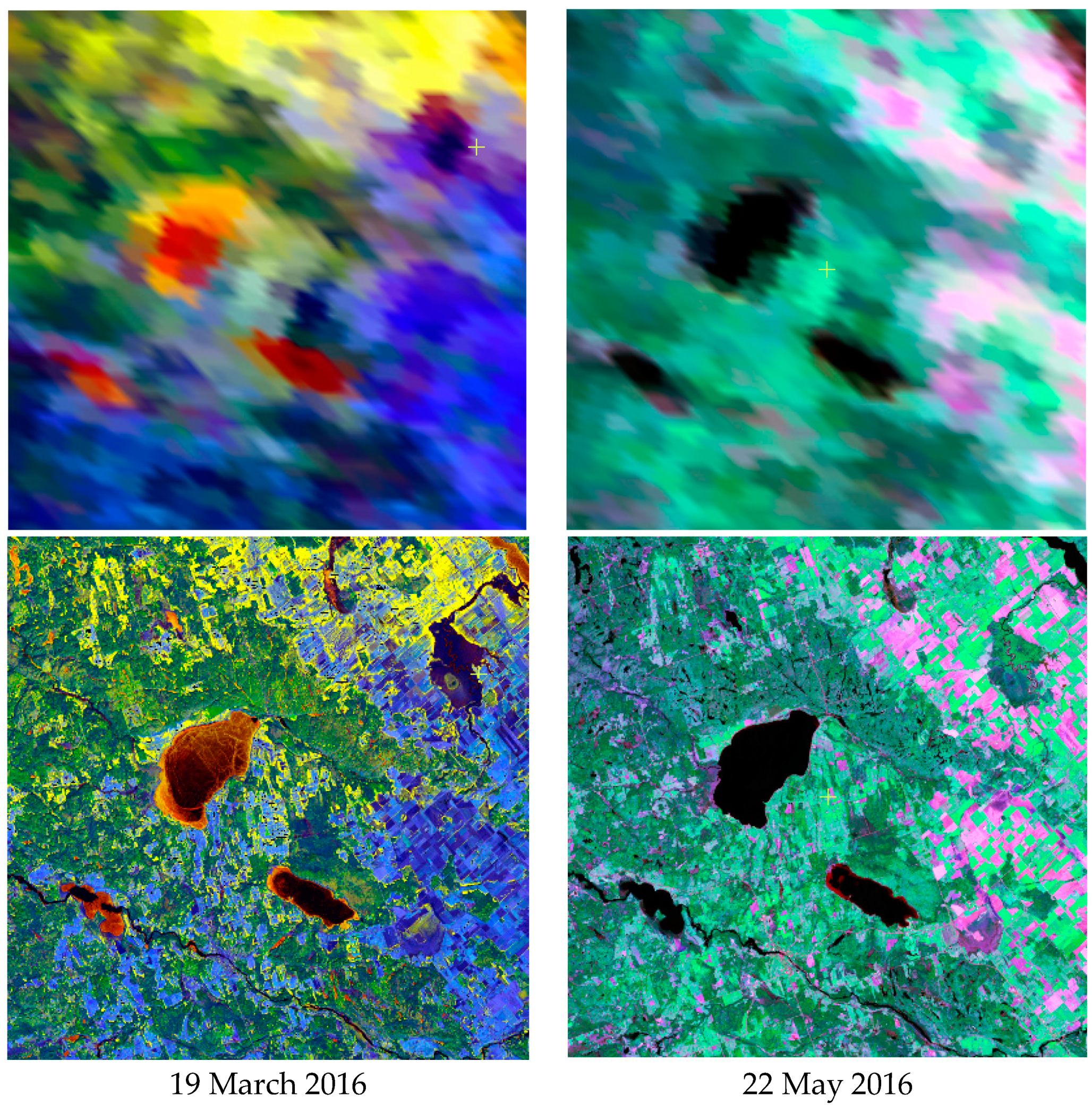
3.2. Study Area and Dataset
4. Results and Discussion
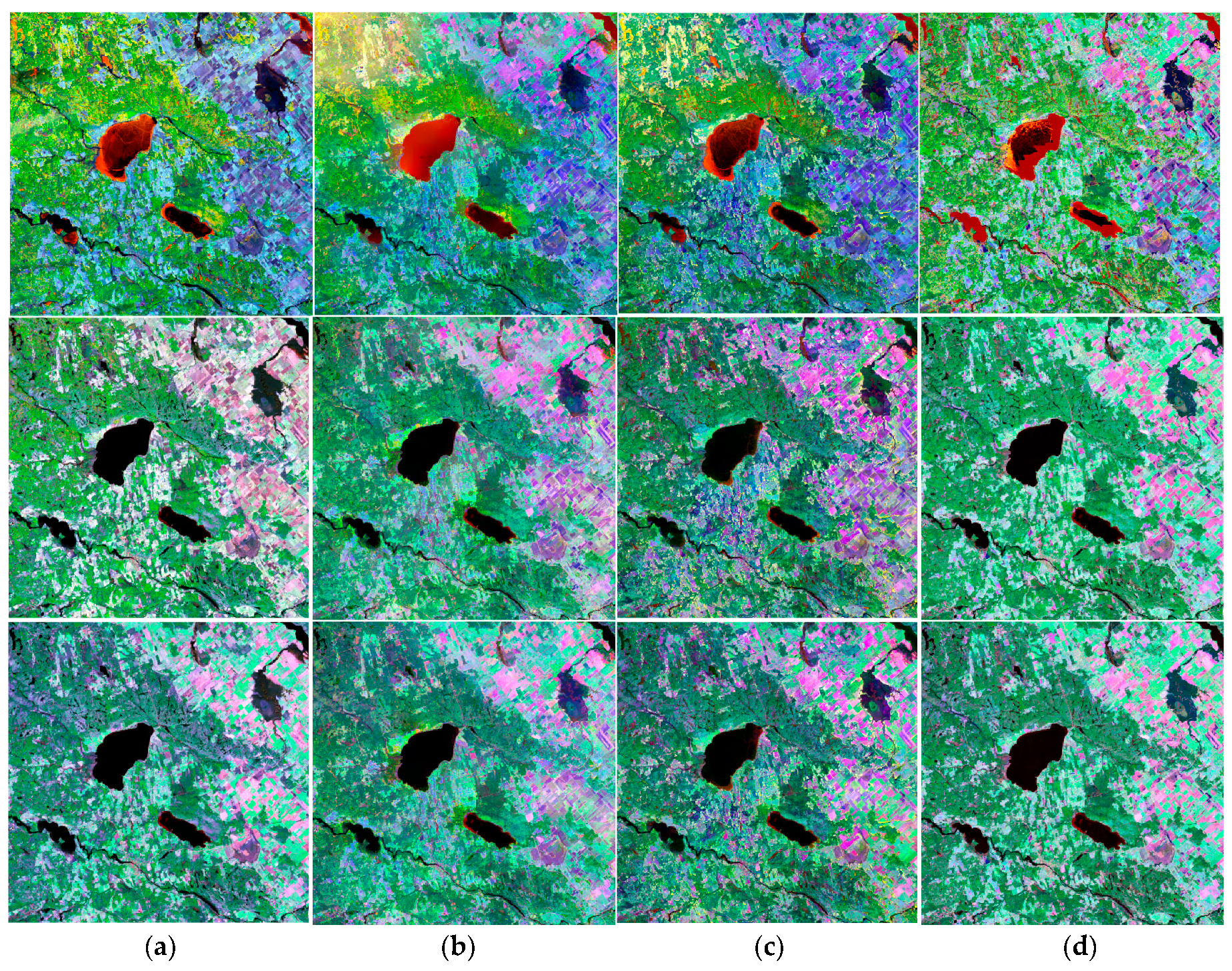
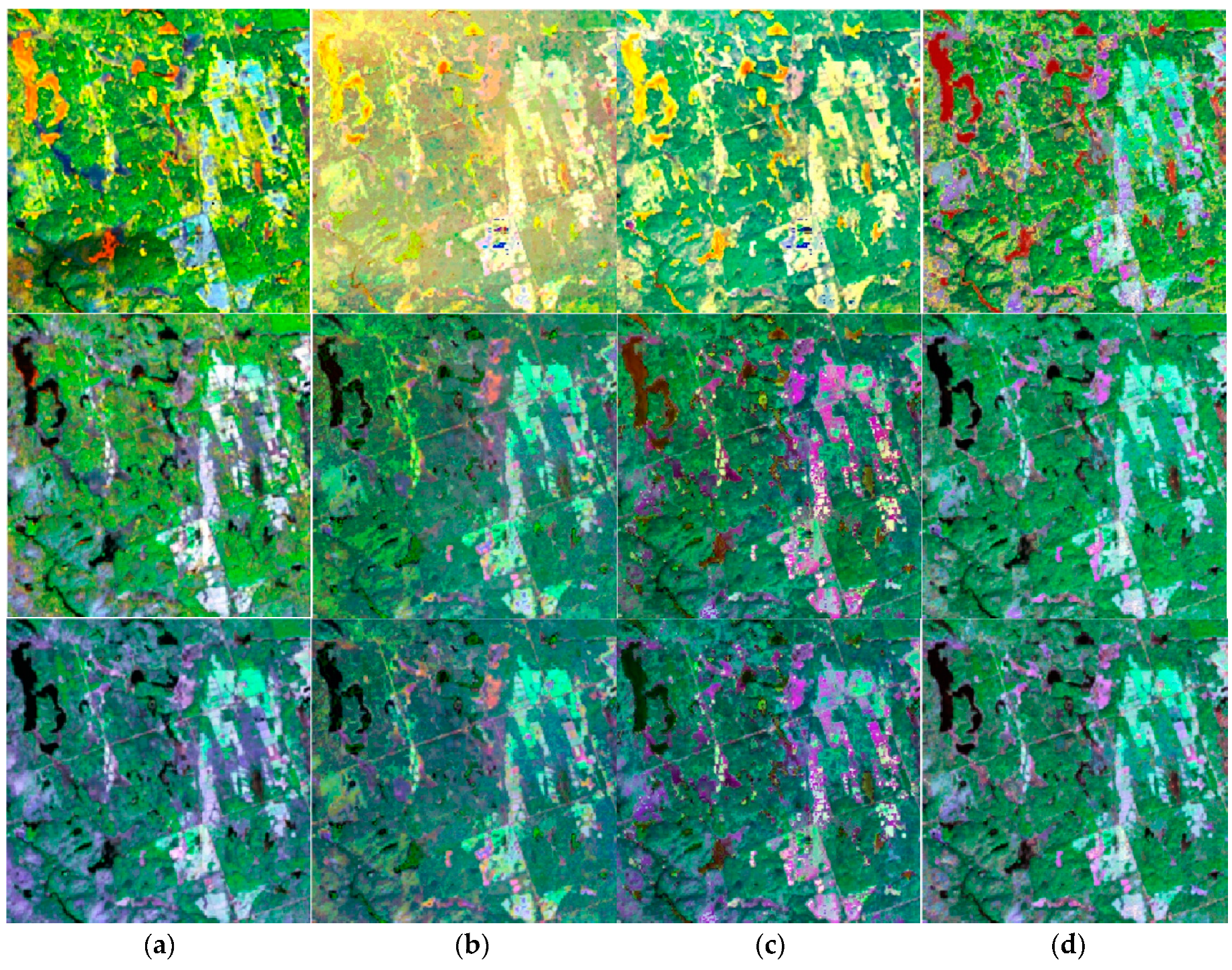
4.1. Visual Comparison of Predicted Landsat-Like Image Time Series against True Landsat Images
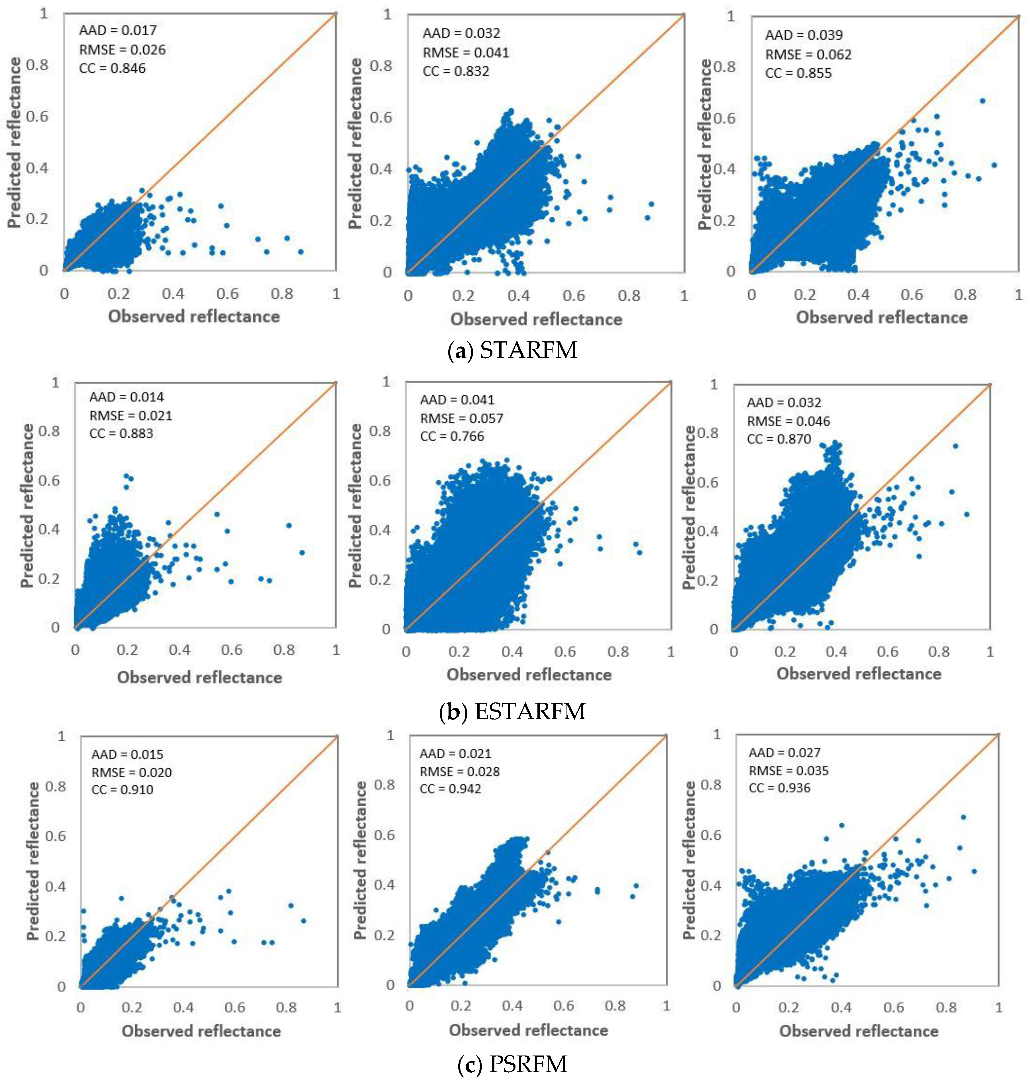
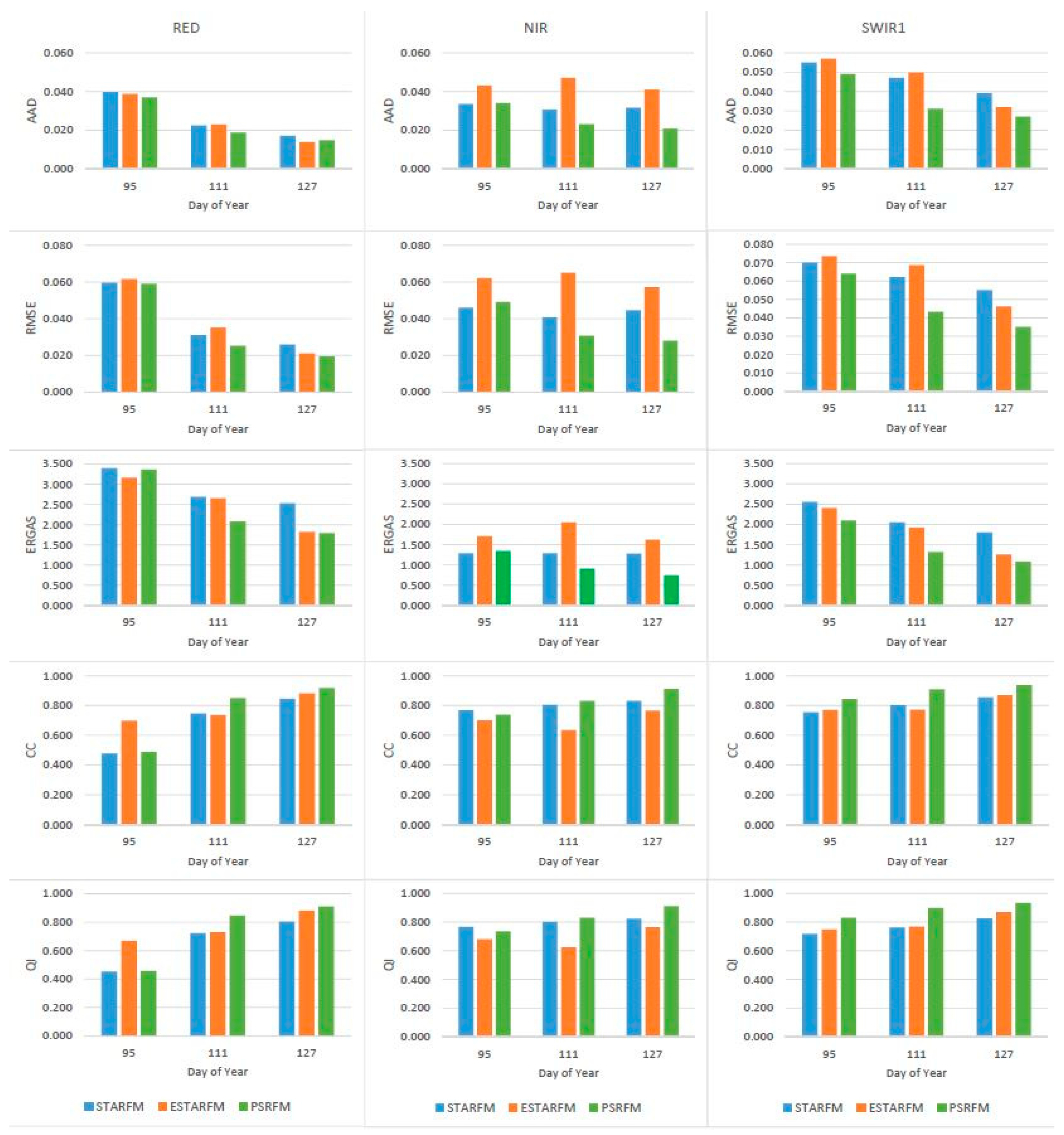
4.2. Quantitative Comparison of the Quality Indices
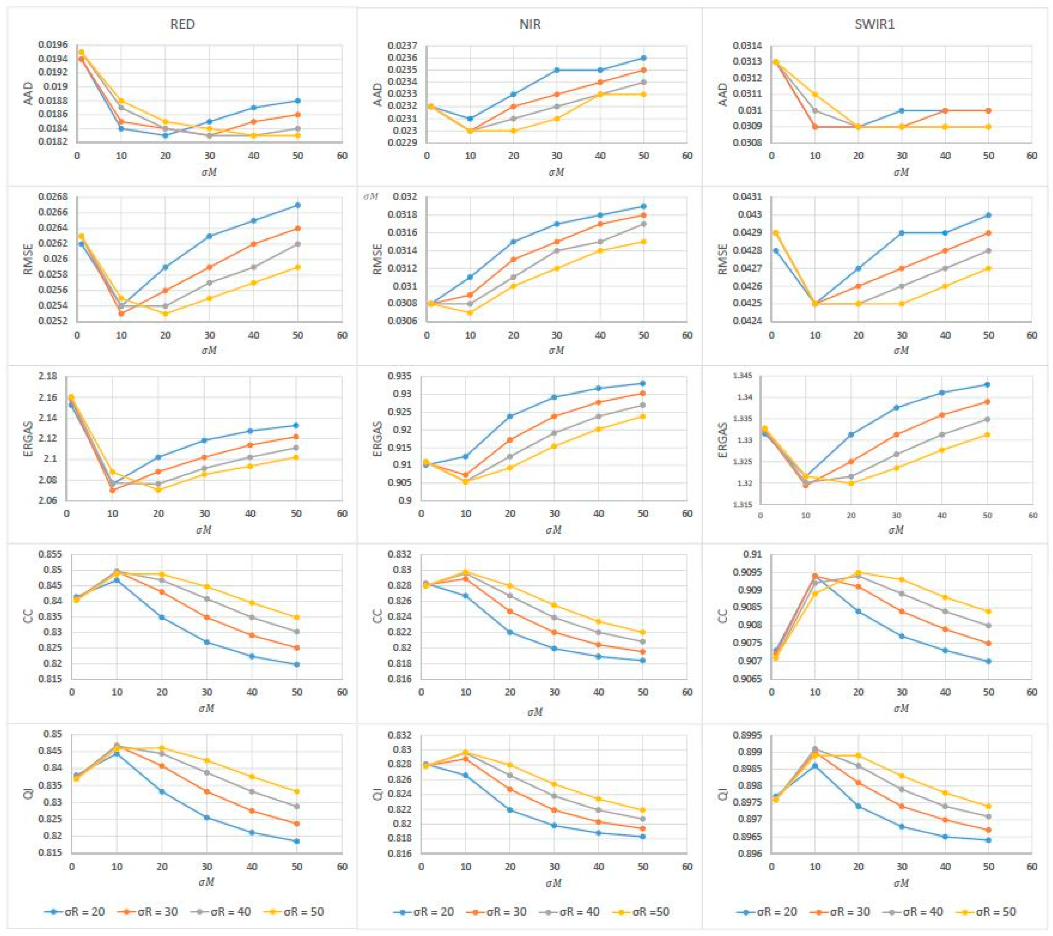
4.3. Uncertainties of the Predicted Landsat-Like Images
5. Conclusions
Author Contributions
Funding
Acknowledgments
Conflicts of Interest
References
- Gao, F.; Masek, J.; Schwaller, M.; Hall, F. On the blending of the Landsat and MODIS surface reflectance: Predicting daily Landsat surface reflectance. IEEE Trans. Geosci. Remote Sens. 2006, 44, 2207–2218. [Google Scholar]
- Zhu, X.; Chen, J.; Gao, F.; Chen, X.; Masek, J.G. An enhanced spatial and temporal adaptive reflectance fusion model for complex heterogeneous regions. Remote Sens. Environ. 2010, 114, 2610–2623. [Google Scholar] [CrossRef]
- Hilker, T.; Wulder, M.A.; Coops, N.C.; Linke, J.; McDermid, G.; Masek, J.G.; Gao, F.; White, J.C. A new data fusion model for high spatial- and temporal-resolution mapping of forest disturbance based on Landsat and MODIS. Remote Sens. Environ. 2009, 113, 1613–1627. [Google Scholar] [CrossRef]
- Zhukov, B.; Oertel, D.; Lanzl, F.; Reinhackel, G. Unmixing-based multisensor multiresolution image fusion. IEEE Trans. Geosci. Remote Sens. 1999, 37, 1212–1226. [Google Scholar] [CrossRef]
- Huang, B.; Zhang, H. Spatio-temporal reflectance fusion via unmixing: Accounting for both phenological and land-cover changes. Int. J. Remote Sens. 2014, 35, 6213–6233. [Google Scholar] [CrossRef]
- Zhu, X.; Helmer, E.H.; Gao, F.; Liu, D.; Chen, J.; Lefsky, M.A. A flexible spatiotemporal method for fusing satellite images with different resolutions. Remote Sens. Environ. 2016, 172, 165–177. [Google Scholar] [CrossRef]
- Hazaymeh, K.; Hassan, Q.K. Spatiotemporal image-fusion model for enhancing temporal resolution of Landsat-8 surface reflectance images using MODIS images. J. Appl. Remote Sens. 2015, 9, 096095. [Google Scholar] [CrossRef]
- Kwan, C.; Budavari, B.; Gao, F.; Zhu, X. A Hybrid Color Mapping Approach to Fusing MODIS and Landsat Images for Forward Prediction. Remote Sens. 2018, 10, 520. [Google Scholar] [CrossRef]
- Wang, J.; Huang, B. A Rigorously-Weighted Spatiotemporal Fusion Model with Uncertainty Analysis. Remote Sens. 2017. [Google Scholar] [CrossRef]
- Song, H.; Huang, B. Spatiotemporal satellite image fusion through one-pair image learning. IEEE Trans. Geosci. Remote Sens. 2013, 51, 1883–1896. [Google Scholar] [CrossRef]
- Emelyanova, I.V.; McVicar, T.R.; Van Niel, T.G.; Li, L.T.; van Dijk, A.I.J.M. Assessing the accuracy of blending Landsat–MODIS surface reflectances in two landscapes with contrasting spatial and temporal dynamics: A framework for algorithm selection. Remote Sens. Environ. 2013, 133, 193–209. [Google Scholar] [CrossRef]
- Hirvonen, R.A. Adjustments by Least Squares in Geodesy and Photogrammetry; Ungar: New York, NY, USA, 1971; 261p, ISBN1 0804443971. ISBN2 978-0804443975. [Google Scholar]
- Wolf, P.R. Survey Measurement Adjustments by Least Squares. In The Surveying Handbook; Springer: Boston, MA, USA, 1995; pp. 383–413. [Google Scholar]
- Dozier, J. Spectral signature of alpine snow cover from the Landsat Thematic Mapper. Remote Sens. Environ. 1989, 28, 9–22. [Google Scholar] [CrossRef]
- Hall, D.K.; Riggs, G.A.; Salomonson, V.V. Development of methods for mapping global snow cover using Moderate Resolution Imaging Spectroradiometer (MODIS) data. Remote Sens. Environ. 1995, 54, 127–140. [Google Scholar] [CrossRef]
- Weier, J.; Herring, D. Measuring Vegetation (NDVI & EVI). 2000. Available online: https://earthobservatory.nasa.gov/Features/MeasuringVegetation/measuring_vegetation_1.php (accessed on 1 December 2017).
- Yengoh, G.T.; Dent, D.; Olsson, L.; Tengberg, A.E.; Tucker, C.J. The Use of the Normalized Difference Vegetation Index (NDVI) to Assess Land Degradation at Multiple Scales: A Review of the Current Status, Future Trends, and Practical Considerations; Lund University Center for Sustainability Studies (LUCSUS); The Scientific and Technical Advisory Panel of the Global Environment Facility (STAP/GEF): Lund, Sweden, 2014. [Google Scholar]
- Zhou, F.; Zhang, A. Methodology for estimating availability of cloud-free image composites: A case study for southern Canada. Int. J. Appl. Earth Observ. Geoinf. 2012, 21, 17–31. [Google Scholar] [CrossRef]
- Zhou, F.; Zhang, A.; Townley-Smith, L. A data mining approach for evaluation of optimal time-series of MODIS data for land cover mapping at a regional level. ISPRS J. Photogramm. Remote Sens. 2013, 84, 114–129. [Google Scholar] [CrossRef]
- Emelyanova, I.; McVicar, T.; Van Niel, T.; Li, L.; Van Dijk, A. Landsat and MODIS Data for the Lower Gwydir Catchment Study Site, v3; Data Collection; CSIRO: Canberra, Australia, 2013. [Google Scholar]
- Gevaert, C.M.; García-Haro, F.J. A comparison of STARFM and an unmixingbased algorithm for Landsat and MODIS data fusion. Remote Sens. Environ. 2015, 156, 34–44. [Google Scholar] [CrossRef]
- Gao, F.; Masek, J.; Wolfe, R.; Huang, C. Building consistent medium resolution satellite data set using moderate resolution imaging spectroradiometer products as reference. J. Appl. Remote Sens. 2010, 4, 043526. [Google Scholar] [CrossRef]
- Vaiopoulos, A.D. Developing Matlab scripts for image analysis and quality assessment. In Proc. SPIE 8181, Earth Resources and Environmental Remote Sensing/GIS Applications II; International Society for Optics and Photonics: Bellingham, WA, USA, 2011; p. 81810B. [Google Scholar] [CrossRef]
- Zhou, W.; Bovik, A.C.; Sheikh, H.R.; Simoncelli, E.P. Image Quality Assessment: From Error Visibility to Structural Similarity. IEEE Trans. Image Process. 2004, 13, 600–612. [Google Scholar] [Green Version]
- Pa, J.; Hegdeb, A.V. A Review of Quality Metrics for Fused Image. Aquat. Procedia 2015, 4, 133–142. [Google Scholar]
- Zhang, Y. Methods for Image Fusion Quality Assessment—A Review, Comparison and Analysis. In Proceedings of the International Achieves of the Photogrammetry, Remote Sensing Information Sciences, Beijing, China, 11–13 July 2008; pp. 1101–1109. [Google Scholar]


| Image Acquisition Date | Landsat-8 OLI | MODIS (MOD09GA) |
|---|---|---|
| 19 March 2016 | Model input (start date) | Model input (start date) |
| 4 April 2016 | For model validation | Model input (for prediction) |
| 20 April 2016 | For model validation | Model input (for prediction) |
| 6 May 2016 | For model validation | Model input (for prediction) |
| 22 May 2016 | Model input (end date) | Model input (end date) |
| Band | Method | AAD | RMSE | ERGAS | ||||||
|---|---|---|---|---|---|---|---|---|---|---|
| Date (Day of Year) | 95 | 111 | 127 | 95 | 111 | 127 | 95 | 111 | 127 | |
| RED | STARFM | 0.040 | 0.023 | 0.017 | 0.060 | 0.031 | 0.026 | 3.397 | 2.688 | 2.529 |
| ESTARFM | 0.039 | 0.023 | 0.014 | 0.062 | 0.035 | 0.021 | 3.162 | 2.656 | 1.824 | |
| PSRFM | 0.037 | 0.019 | 0.015 | 0.059 | 0.025 | 0.020 | 3.361 | 2.077 | 1.792 | |
| NIR | STARFM | 0.034 | 0.031 | 0.032 | 0.046 | 0.041 | 0.045 | 1.286 | 1.286 | 1.277 |
| ESTARFM | 0.043 | 0.047 | 0.041 | 0.062 | 0.065 | 0.057 | 1.705 | 2.049 | 1.622 | |
| PSRFM | 0.034 | 0.023 | 0.021 | 0.049 | 0.031 | 0.028 | 1.339 | 0.906 | 0.743 | |
| SWIR1 | STARFM | 0.055 | 0.047 | 0.039 | 0.070 | 0.062 | 0.055 | 2.557 | 2.051 | 1.805 |
| ESTARFM | 0.057 | 0.050 | 0.032 | 0.074 | 0.069 | 0.046 | 2.406 | 1.922 | 1.257 | |
| PSRFM | 0.049 | 0.031 | 0.027 | 0.064 | 0.043 | 0.035 | 2.095 | 1.320 | 1.081 | |
| AVERAGE | STARFM | 0.043 | 0.033 | 0.029 | 0.059 | 0.045 | 0.042 | 2.413 | 2.008 | 1.870 |
| ESTARFM | 0.046 | 0.040 | 0.029 | 0.066 | 0.056 | 0.042 | 2.425 | 2.209 | 1.568 | |
| PSRFM | 0.040 | 0.024 | 0.021 | 0.057 | 0.033 | 0.027 | 2.265 | 1.434 | 1.205 | |
| Band | Method | CC | QI | ||||
|---|---|---|---|---|---|---|---|
| Date (Day of Year) | 95 | 111 | 127 | 95 | 111 | 127 | |
| RED | STARFM | 0.478 | 0.746 | 0.846 | 0.453 | 0.722 | 0.805 |
| ESTARFM | 0.697 | 0.735 | 0.883 | 0.669 | 0.729 | 0.882 | |
| PSRFM | 0.487 | 0.850 | 0.917 | 0.456 | 0.847 | 0.911 | |
| NIR | STARFM | 0.767 | 0.804 | 0.832 | 0.767 | 0.801 | 0.823 |
| ESTARFM | 0.700 | 0.633 | 0.766 | 0.680 | 0.623 | 0.764 | |
| PSRFM | 0.738 | 0.830 | 0.911 | 0.736 | 0.830 | 0.910 | |
| SWIR1 | STARFM | 0.755 | 0.802 | 0.855 | 0.717 | 0.762 | 0.826 |
| ESTARFM | 0.769 | 0.772 | 0.870 | 0.749 | 0.768 | 0.869 | |
| PSRFM | 0.844 | 0.909 | 0.938 | 0.829 | 0.899 | 0.934 | |
| AVERAGE | STARFM | 0.667 | 0.784 | 0.844 | 0.646 | 0.761 | 0.818 |
| ESTARFM | 0.722 | 0.713 | 0.840 | 0.699 | 0.706 | 0.838 | |
| PSRFM | 0.690 | 0.863 | 0.922 | 0.674 | 0.859 | 0.918 | |
| Band | Forward | Backward | Smoothed | Variations with Various | |
|---|---|---|---|---|---|
| 1 | RED | 40.3839 | 40.0100 | 31.7790 | 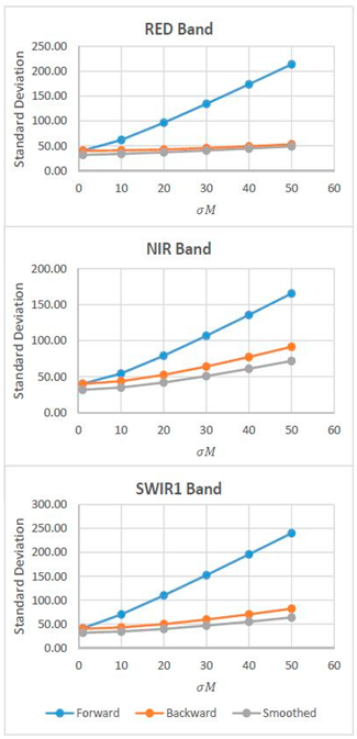 |
| NIR | 40.2222 | 40.0493 | 31.7836 | ||
| SWIR1 | 41.1148 | 40.0384 | 31.7753 | ||
| AVERAGE | 40.5736 | 40.0326 | 31.7793 | ||
| 10 | RED | 61.7432 | 40.6861 | 33.7521 | |
| NIR | 54.3945 | 43.6591 | 34.9295 | ||
| SWIR1 | 70.0981 | 42.8367 | 34.2172 | ||
| AVERAGE | 62.0786 | 42.3940 | 34.2996 | ||
| 20 | RED | 96.4420 | 42.5392 | 36.9317 | |
| NIR | 79.0727 | 52.4617 | 41.8778 | ||
| SWIR1 | 109.9881 | 49.8445 | 39.6621 | ||
| AVERAGE | 95.1676 | 48.2818 | 39.4905 | ||
| 30 | RED | 134.3868 | 45.3425 | 40.5261 | |
| NIR | 106.7142 | 64.0919 | 50.8407 | ||
| SWIR1 | 152.3086 | 59.3361 | 46.7589 | ||
| AVERAGE | 131.1366 | 56.2568 | 46.0539 | ||
| 40 | RED | 173.7371 | 48.8890 | 44.5579 | |
| NIR | 135.7250 | 77.2962 | 60.9896 | ||
| SWIR1 | 195.8454 | 70.3035 | 54.8945 | ||
| AVERAGE | 168.4448 | 65.4926 | 53.4806 | ||
| 50 | RED | 213.8119 | 53.0122 | 48.8832 | |
| NIR | 165.5597 | 91.4239 | 71.8612 | ||
| SWIR1 | 240.0988 | 82.1800 | 63.7070 | ||
| AVERAGE | 206.4901 | 75.5387 | 61.4838 |
| Band | AAD | RMSE | ERGAS | CC | QI | |
|---|---|---|---|---|---|---|
| RED | 1 | 0.0195 | 0.0263 | 2.1600 | 0.8404 | 0.8370 |
| 10 | 0.0187 | 0.0254 | 2.0772 | 0.8497 | 0.8467 | |
| 20 | 0.0184 | 0.0254 | 2.0763 | 0.8468 | 0.8444 | |
| 30 | 0.0183 | 0.0257 | 2.0914 | 0.8408 | 0.8388 | |
| 40 | 0.0183 | 0.0259 | 2.1022 | 0.8348 | 0.8332 | |
| 50 | 0.0184 | 0.0262 | 2.1113 | 0.8302 | 0.8288 | |
| NIR | 1 | 0.0232 | 0.0308 | 0.9109 | 0.8280 | 0.8279 |
| 10 | 0.0230 | 0.0308 | 0.9055 | 0.8296 | 0.8296 | |
| 20 | 0.0231 | 0.0311 | 0.9125 | 0.8267 | 0.8266 | |
| 30 | 0.0232 | 0.0314 | 0.9191 | 0.8239 | 0.8238 | |
| 40 | 0.0233 | 0.0315 | 0.9238 | 0.8220 | 0.8219 | |
| 50 | 0.0234 | 0.0317 | 0.9270 | 0.8208 | 0.8207 | |
| SWIR1 | 1 | 0.0313 | 0.0429 | 1.3326 | 0.9071 | 0.8976 |
| 10 | 0.0310 | 0.0425 | 1.3201 | 0.9092 | 0.8991 | |
| 20 | 0.0309 | 0.0425 | 1.3215 | 0.9094 | 0.8986 | |
| 30 | 0.0309 | 0.0426 | 1.3267 | 0.9089 | 0.8979 | |
| 40 | 0.0309 | 0.0427 | 1.3313 | 0.9084 | 0.8974 | |
| 50 | 0.0309 | 0.0428 | 1.3349 | 0.9080 | 0.8971 | |
| AVERAGE | 1 | 0.0247 | 0.0333 | 1.4679 | 0.8585 | 0.8542 |
| 10 | 0.0242 | 0.0329 | 1.4343 | 0.8628 | 0.8585 | |
| 20 | 0.0241 | 0.0330 | 1.4368 | 0.8610 | 0.8565 | |
| 30 | 0.0242 | 0.0332 | 1.4458 | 0.8579 | 0.8535 | |
| 40 | 0.0242 | 0.0334 | 1.4524 | 0.8551 | 0.8508 | |
| 50 | 0.0243 | 0.0335 | 1.4578 | 0.8530 | 0.8488 |
© 2018 by the authors. Licensee MDPI, Basel, Switzerland. This article is an open access article distributed under the terms and conditions of the Creative Commons Attribution (CC BY) license (http://creativecommons.org/licenses/by/4.0/).
Share and Cite
Zhong, D.; Zhou, F. A Prediction Smooth Method for Blending Landsat and Moderate Resolution Imagine Spectroradiometer Images. Remote Sens. 2018, 10, 1371. https://doi.org/10.3390/rs10091371
Zhong D, Zhou F. A Prediction Smooth Method for Blending Landsat and Moderate Resolution Imagine Spectroradiometer Images. Remote Sensing. 2018; 10(9):1371. https://doi.org/10.3390/rs10091371
Chicago/Turabian StyleZhong, Detang, and Fuqun Zhou. 2018. "A Prediction Smooth Method for Blending Landsat and Moderate Resolution Imagine Spectroradiometer Images" Remote Sensing 10, no. 9: 1371. https://doi.org/10.3390/rs10091371
APA StyleZhong, D., & Zhou, F. (2018). A Prediction Smooth Method for Blending Landsat and Moderate Resolution Imagine Spectroradiometer Images. Remote Sensing, 10(9), 1371. https://doi.org/10.3390/rs10091371