1. Introduction
With the rapid development of sensor technology and modern communications, we are now entering a multi-sensor era. Different sensors capture different features, which are useful for a variety of applications, including multi-sensor image registration and fusion [
1,
2,
3] and pedestrian detection [
4,
5,
6]. However, the non-linear radiation/intensity variations between multi-sensor images result in the local feature description being a challenging task [
7,
8,
9,
10].
The traditional approaches based on histograms of oriented gradient descriptors such as scale-invariant feature transform (SIFT) [
11] and speeded-up robust features (SURF) [
12] perform well on single-sensor images, but generate only a few correct mappings when dealing with multi-sensor images. To address this issue, researchers have proposed many techniques to adapt descriptors based on SIFT/SURF to multi-sensor images. Approaches such as the partial intensity invariant feature descriptor (PIIFD) [
13], R-SIFT [
14] orientation-restricted SIFT (OR-SIFT) [
15], and multimodal SURF (MM-SURF) [
16] use gradient orientation modification to limit the gradient orientation to (0, pi) on the basis of the intensity reversal in certain areas. Saleem et al. [
17] proposed NG-SIFT, which employs a normalized gradient to construct the feature vectors, and it was found that NG-SIFT outperformed SIFT on visible and near-infrared images.
Even though these descriptors perform slightly better than the traditional descriptors, the number of mismatches increases due to the orientation reversal, and the total number of matched points is still low. This is because the description ability of these descriptors relies on a linear relationship between images, and they are not appropriate for the significant non-linear intensity differences caused by the radiometric variations between multi-sensor images.
Some descriptors have been designed based on the distribution of edge points, which can be regarded as the common features of multi-sensor images. Aguilera et al. [
18] proposed the edge-oriented histogram (EOH) descriptor for multispectral images. Li et al. [
19] assigned the main orientation computed with PIIFD to EOH for increased robustness to rotational invariance. Zhao et al. [
20] used edge lines for a better matching precision. Shi et al. [
21] combined shape context with the DAISY descriptor in a structural descriptor for multispectral remote sensing image registration; however, all the edge points are constrained by contrast and threshold values [
22]. Other descriptors have been proposed, based on local self-similarity (LSS) and its extension for multispectral remote sensing images [
5,
6,
7,
23], but the size of the LSS region contributes much to the descriptor’s capability. Furthermore, LSS and its extensions usually result in a low number of correctly matched points.
Due to the differences in multi-sensor imaging principles, the intensities among multi-sensor images present non-linear radiation variations, resulting in the above descriptors relying on gradient-based linear intensity variations, i.e., spatial domain information, not performing well for multi-sensor images. In addition to the spatial domain, images can be decomposed into amplitude and phase information by Fourier transform in the frequency domain. The ability of a descriptor can be evaluated by “repeatability” and “distinctiveness”, and a trade-off is often made between these measures [
19]. To obtain as much useful information as possible from the images is the goal of a descriptor. More information can be obtained by convolving the images using multi-scale and multi-oriented Gabor-based filters, including the Gabor filter and log-Gabor filter.
The Gabor filter responses are invariant to illumination variations [
24,
25], and the multi-oriented magnitudes transmit useful shape information [
26,
27]. Since the log-Gabor filters basically consist of a logarithmic transformation of the Gabor domain, researchers have proposed descriptors based on the amplitudes of log-Gabor coefficients. The phase congruency and edge-oriented histogram descriptor (PCEHD) [
28] combines spatial information (EOH) and frequency information (the amplitude of the log-Gabor coefficients). The log-Gabor histogram descriptor (LGHD) [
29] uses multi-scale and multi-oriented log-Gabor filters instead of the multi-oriented Sobel descriptor, and it divides the region around the point of interest into sub-regions (similar to SIFT with 4 × 4). LGHD has been used to match images with non-linear intensity variations, including visible and thermal infrared images, and has outperformed SIFT, GISIFT [
30], EOH [
18], and PCEHD. However, LGHD is time-consuming due to its multi-scale computation. Cristiano et al. [
31] proposed the multispectral feature descriptor (MFD), which computes the descriptors using fewer log-Gabor filters and, as a result, has a computational efficiency that is better than that of LGHD.
Oppenheim et al. [
32] analyzed the function of the phase information, and discovered that phase information is even more important than amplitude information for the preservation of image features. The phase congruency detector is a feature detector based on the local phase information of images. Kovesi et al. [
33] proposed a measure of phase congruency that is independent of the overall magnitude of the signal, making it invariant to variations in image illumination and/or contrast. Furthermore, phase congruency is a dimensionless quantity. Therefore, a number of researchers have proposed methods for feature description based on phase congruency, for applications such as template matching for multi-sensor remote sensing images [
34,
35] and pedestrian detection [
36,
37].
The distribution of the high-frequency components of log-Gabor filters has been verified to be robust to non-linear intensity variations [
29,
31], and phase congruency has been successfully used for multispectral image template matching [
34,
35,
36,
37]. This makes us think that a descriptor combining phase congruency and the distribution of the high-frequency components would be more efficient to capture the common information of multi-sensor images, which is the idea behind the proposed approach.
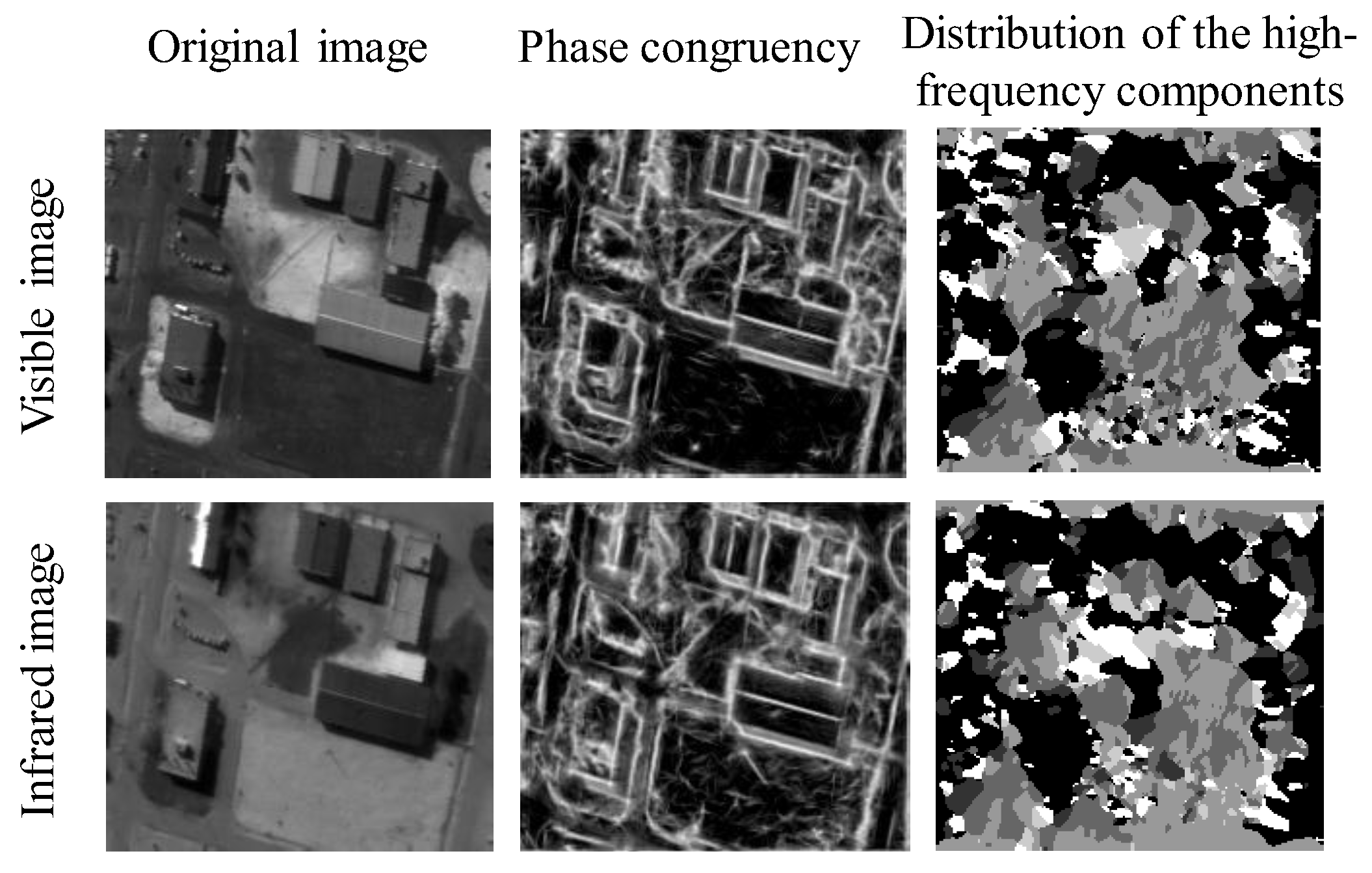
Figure 1 shows a comparison between phase congruency and the distribution of the high-frequency components for a pair of visible and infrared remote sensing images. Vertically, the phase congruency and the distribution of the high-frequency components are similar for the visible and infrared images, even with the non-linear intensity changes existing between the visible and infrared images. Horizontally, the phase congruency is more like the enhanced edges of an image, and the distribution of the high-frequency components is more like the coarse texture of the image.
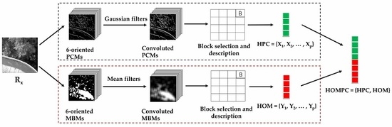
In this paper, a novel descriptor named the histograms of oriented magnitude and phase congruency (HOMPC) combining the histograms of oriented magnitude (HOM) and the histograms of oriented phase congruency (HPC) is proposed. The HOM and HPC can be efficiently calculated in a dense manner over the local regions of the images through a convolution operation. The HOMPC descriptor reflects the structural and shape properties of local regions, which are relatively independent of the particular intensity distribution pattern across two local regions. To the best of our knowledge, we are the first to combine magnitude and phase congruency information to construct a local feature descriptor to capture the common information of multi-sensor images with non-linear radiation variations.
The main contributions of this paper are as follows:
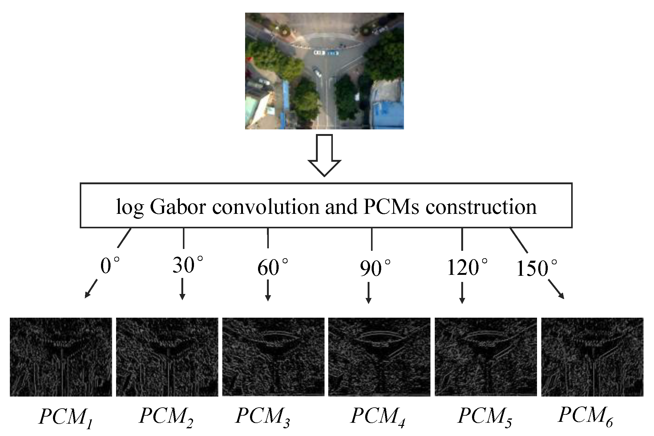
We propose oriented phase congruency maps (PCMs) and oriented magnitude binary maps (MBMs) based on log-Gabor filters;
we have designed a fast method to construct feature vectors through a convolution operation based on the PCMs and MBMs;
we have developed a novel local feature descriptor based on the magnitude and phase congruency information to capture more common structural and shape properties.
The rest of this paper is organized as follows:
Section 2 proposes the HOMPC descriptor based on the HOM and HPC.
Section 3 introduces the experimental setup.
Section 4 analyzes the parameter sensitivity and the advantages of combining the HOM and HPC and describes the comparison of the proposed HOMPC descriptor with the current state-of-art descriptors.
Section 5 presents the conclusions and recommendations for future work.
3. Experimental Setup
The main contribution of this paper is that we proposed a new descriptor to solve the local region feature description problem of multi-sensor images with non-linear radiation variations. In this section, the experimental setup is presented to test our proposed HOMPC descriptor.
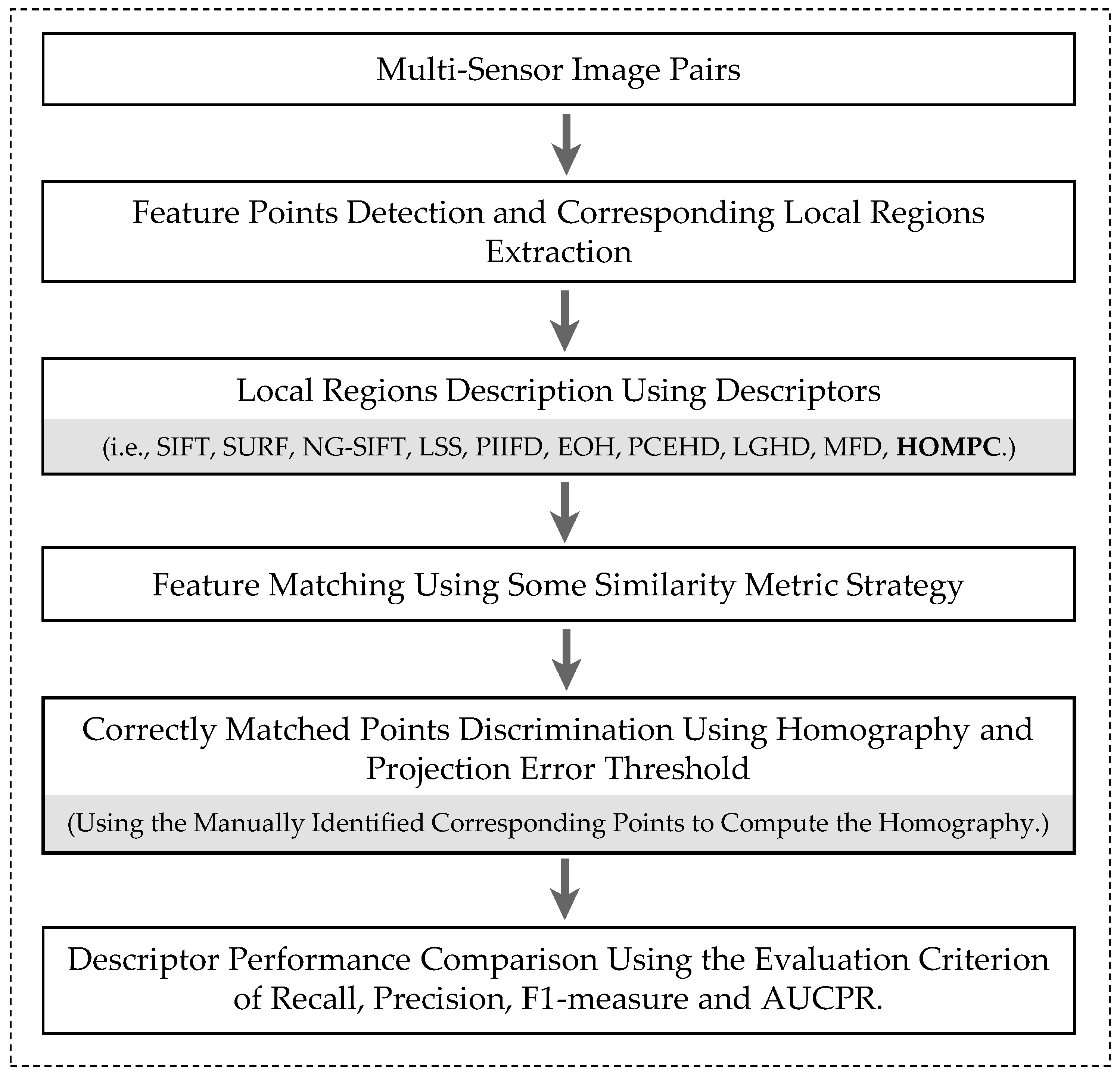
Figure 7 shows the flowchart to evaluate the descriptor performance in our experiments. In order to evaluate the performance of descriptors, some pair of multi-sensor images are chosen and the feature points are detected firstly. Then, the local regions corresponding to the feature points are described using descriptors, and the feature matching is completed with some similarity metric. Then, the correctly matched points and falsely matched points are classified by using the homography and projection error. The homography is calculated by using the manually identified corresponding points of the pair of multi-sensor images. Since two important indicators for evaluating descriptor performance are “repeatability” and “distinctiveness” [
19], we finally selected precision and recall to verify the “distinctiveness” and “repeatability” of descriptors, respectively. The F1-measure and area under precision-recall curves (AUCPR) are used to verify the comprehensive performance of precision and recall. A more detailed introduction of the feature detection method is presented in
Section 3.1. The details of the feature descriptors are supplied in
Section 3.2, and the evaluation criteria and datasets are provided in
Section 3.3 and 3.4, respectively. The parameter settings in our experiments are listed in
Section 3.5.
3.1. Feature Detection
The feature detection is the preprocessing for local regions description. Saleem et al. [
43] compared different feature detectors and descriptors on four multi-sensor images, and the experimental results showed that the corner feature detectors (e.g., Harris, FAST [
44]) could obtain more correct matches than blob detectors (e.g., SIFT, SURF) for multi-sensor images. The aim is to verify the performance of descriptors, and the more the number of the initial corresponding correct matching points, the more beneficial to verify the performance of descriptors.
In our experiment, we selected the phase congruency corner detector [
33] to detect feature points. Different from the gradient-based corner detectors (e.g., Harris, FAST), the phase congruency corner detector is based on phase information, which is invariant to contrast and illumination changes. In addition, the non-maximum suppression method was used to extract local (3 × 3) significant points. After then, we could obtain more initial corresponding correct matches to verify the descriptor performance. We detected a total of 2500 points for each image of multi-sensor images. However, image texture and scene complexity affect the final detected points.
3.2. Feature Descriptors
In addition to verifying the performance of our descriptors on multi-sensor images, we need to compare our proposed descriptors with classic descriptors through multi-sensor images. We selected some representative descriptors, e.g., SIFT [
11], SURF [
12], LSS [
5], EOH [
18], and five state-of-the-art descriptors named NG-SIFT [
17], PIIFD [
13], PCEHD [
28], LGHD [
29], and MFD [
31] to compare with our proposed HOMPC descriptor. We programmatically implemented NG-SIFT and MFD descriptors and tried to maximize their performance using MATLAB. Whereas the implementation of the remaining algorithms is available online with MATLAB.
3.3. Evaluation Criteria
The ability of a descriptor can be evaluated by “repeatability” and “distinctiveness” [
19]. The common evaluation criteria, including recall and precision from [
45], F1-measure, and AUCPR from [
17], and projection error from [
43,
46] were chosen to measure the descriptor performance.
Projection error is a Euclidian distance between the reference and projected image feature points. The projected image feature points are transformed by using a known homography H, which is computed by manually selecting the corresponding points of reference and target images. If the projection error of one pair of points is less than some threshold, we regard it as the correctly matched points, otherwise, the falsely matched points.
Descriptor matching is carried out with MATLAB implementation of ‘matchFeatures’ function, which uses Sum of absolute differences (SAD), sum of squared differences (SSD) or Hamming distance, between descriptor vectors. As introduced in the document of MATLAB, the default SSD metric is suitable for non-binary feature descriptors, so the SSD was selected as the feature similar metric. A reference point of interest is defined as being matched to a test interest point if:
where
is the Euclidean distance;
is the feature vector of the reference point of interest;
are the two feature vectors of points to be matched and
is the second-closest neighbor to
. The “
thresh” is the threshold of the nearest neighbor distance ratio (NNDR). The smaller value of “
thresh” means tighter matching criterion. The “
thresh” was set to 0.8–1.0 at an interval of 0.05 in our experiments to test the matching results with different conditions.
Recall is the ratio of the number of correctly matched point pairs of the matching results and the total number of existing correct-match point pairs of the initial match point sets. assesses the accuracy of the returning ground-truth image pairs.
Precision is the ratio of the number of correctly matched point pairs of the matching result and the sum of the number of correctly and falsely matched point pairs of the matching results. calculates the ability to exclude false positives.
F1-measure captures the fitness of the ground truth and detected points by jointly considering the
Recall and
Precision. The F1-measure [
31,
47] is calculated as follows:
AUCPR is the area under the precision-recall curve [
17], which was also computed for the performance comparison.
To better express the universality of the proposed HOMPC descriptor and the other descriptors, the average precision and recall were calculated from the multi-sensor image pairs of each dataset according to different NNDR thresholds. The F1-measure and AUCPR were calculated from the average precision and recall values.
3.4. Datasets
The descriptor we designed was mainly to solve the problem of common feature description between images with nonlinear radiation differences of multi-sensor images. The image datasets used in our experiments should be acquired from different sensor devices. Three datasets (CVC dataset, UAV dataset, and SAT dataset) were chosen based on the height of the remote sensing platform. Samples from these datasets are shown in
Figure 8.
The CVC dataset includes 44 RGB/LWIR (longwave infrared) [
29,
48] outdoor image pairs and 100 VS/LWIR (visible and longwave infrared) [
18,
49] outdoor images of different urban scenarios. These image pairs were captured using the color cameras and infrared camera. For a more detailed description with the two cameras, please refer to [
49].
The UAV dataset includes 27 RGB/LWIR outdoor images specially acquired by ourselves from an unmanned aerial vehicle (UAV) (DJI M100) using the optical and thermal infrared cameras. The image resolution of the thermal infrared camera is 640 × 480, and the wavelength range is 8–14 μm. The optical camera is industrial grade. Its pixels size is 5.0 μm × 5.2 μm and image resolution is 1280 × 720.
The SAT dataset contains six pairs of remote sensing satellite images. The image pairs cover a variety of low-, medium-, and high-resolution remote sensing satellite images with a ground sample distance (GSD) from 0.5 to 30 m. The supported images came from different satellites. The multi-temporal satellite images were also included. For a more detailed description for the six pairs of images, please refer to [
7].
Similar to LGHD and MFD, it should be noted that the proposed HOMPC descriptor is designed for non-linear radiation variations between multi-sensor images, and we do not consider the geometric changes of rotation and scale variations. Therefore, the multi-sensor remote sensing image pairs should be rectified without significant rotation or scaling transformation. In fact, the image pairs of the CVC dataset were rectified and aligned so that matches should be found in horizontal lines. The image pairs of the UAV dataset included small projective changes, in addition to small rotation transformation. The image pairs of the SAT dataset had been rectified to the same scale size based on GSD values.
3.5. Parameter Settings
The patch size of the proposed HOMPC descriptor was assigned to 80 × 80, the same as EOH, LGHD, and MFD. The patch sizes of other descriptors were set by default. We use NS = 4 and NO = 6 to express the number of convolution scales and orientations of the log-Gabor filter in the proposed method. The projection error threshold was assigned to 5 for all three datasets. The larger the projection error threshold, the more correctly matched points for the recall and precision calculations. The threshold of NNDR was assigned to the range 0.8–1.0 with an interval of 0.05 in our experiments, where a smaller value means a tighter matching criterion.
4. Experimental Results and Discussion
The parameters of the proposed method are discussed in
Section 4.1. The advantages of combining the phase information and magnitude information are evaluated and discussed in
Section 4.2. The superiority of the proposed HOMPC descriptor over the current state-of-the-art local feature descriptors is evaluated and discussed in
Section 4.3 and
Section 4.4.
4.1. Parameter Study
The proposed HOMPC method contains four main parameters, namely,
NS,
NO,
CL, and
IL. As mentioned
NS = 4 and
NO = 6 are used to express the number of convolution scales and orientations of the log-Gabor filter in the proposed method. Parameter
CL is the size of the local cell patch (cell size) used for the cell description. If the cell size is too small, it will contain insufficient information with which it is difficult to reflect the distinctiveness of the feature. In contrast, if the cell size is too large, it is easily affected by the local geometric distortion. Parameter
IL is the number of intervals between blocks. In general, the smaller the number of intervals, the richer the information of the constructed HOM and HPC, and the poorer the robustness and the higher the dimension of the feature vectors. In contrast, if the number of intervals is too large, the HOMPC descriptor will contain less information, which will also affect the distinctiveness of the feature. Therefore, suitable parameters are very important. In this section, we describe the parameter study and sensitivity analysis based on the 44RGB/LWIR dataset. We designed two independent experiments to learn parameters
CL and
IL, where each experiment had only one parameter as a variable, with the other parameters as fixed values. The experimental setup details are summarized in
Table 1. For each parameter, we use the average precision and recall, F1-measure, and AUCPR as the evaluation metric. The experimental results are reported in
Figure 9 and
Figure 10;
Table 2 and
Table 3.
From the experimental results, we can infer that: (1) Larger values of
CL mean that the cell size information is richer, and thus more AUCPR values and F1-measure scores can be obtained; however, due to the effect of local geometric distortion, the AUCPR values and F1-measure scores will decrease as the value of
CL increases. As shown in
Table 2 and
Figure 9, the HOMPC descriptor achieves the best performance when
CL = 20. Therefore, we set
CL = 20; (2) From
Table 2 and
Figure 9, we can see that large values of
IL result in a poor performance, while small values mean richer information of the constructed HOM and HPC feature vectors; however, smaller values of
IL also mean that the distinctiveness of the proposed HOMPC feature vector increases, which will decrease the robustness and increase the dimension of the proposed feature vectors. As shown in
Table 3 and
Figure 10, when
IL = 8, HOMPC achieves the best performance. Therefore, we set
IL = 8. Based on the experimental results and analysis, these parameters were fixed to
CL = 20 and
IL = 8 in the experiments.
4.2. The Advantages of the Magnitude and Phase Congruency Information Combination
To verify the advantages of combining the magnitude and phase congruency information, the HOMPC descriptor was compared with HPC and HOM based on the 44RGB/LWIR dataset. The variable parameters were set as suggested in
Section 4.1. The average precision and recall results, as well as the F1-measure and AUCPR results of HOMPC, HOM, and HPC are given in
Figure 11 and
Figure 12.
Since the larger the NNDR threshold, the looser the matching metric for the point matching, the average curves of the recall values of HOMPC, HOM, and HPC are raised while the average curves of the precision values are decreased as the NNDR threshold increases, as shown in
Figure 11. This indicates that the average curve of the recall values of the HOMPC descriptor is much better than the curves of HOM and HPC, and the average curve of the precision values of HOMPC is similar to that of HPC, but is much better than that of HOM. As it is known that the phase information contributes more to the preservation of image features than amplitude information, the precision values of HPC are much better than those of HOM. However, the distribution of the high-frequency component information also contributes to the shape of the objects, and we can see that the recall values of HOM are similar to those of HPC. After combining HOM and HPC, HOMPC keeps the distinctiveness of HPC, but also increases the repeatability by adding HOM.
A comprehensive analysis of the average recall and precision is provided in
Table 4 and
Figure 12. The average PR curves, F1-measure curves, and AUCPR values also indicate that HOMPC outperforms HOM and HPC.
It is found that the advantages of combining the magnitude and phase congruency information are significant. More particularly, it is the phase congruency information that makes a greater contribution to the distinctiveness of HOMPC, and the magnitude information adds to the repeatability of HOMPC.
4.3. Descriptor Comparison
We used the three datasets introduced in
Section 3.4, i.e., CVC dataset, UAV dataset and SAT dataset to compare the proposed HOMPC descriptor with the current state-of-the-art local feature descriptors of SIFT [
11], SURF [
12], NG-SIFT [
17], LSS [
5], PIIFD [
13], EOH [
18], PCEHD [
28], LGHD [
29], and MFD [
31] in terms of the average precision and recall, as well as F1-measure and AUCPR.
4.3.1. Results Obtained with the CVC Dataset
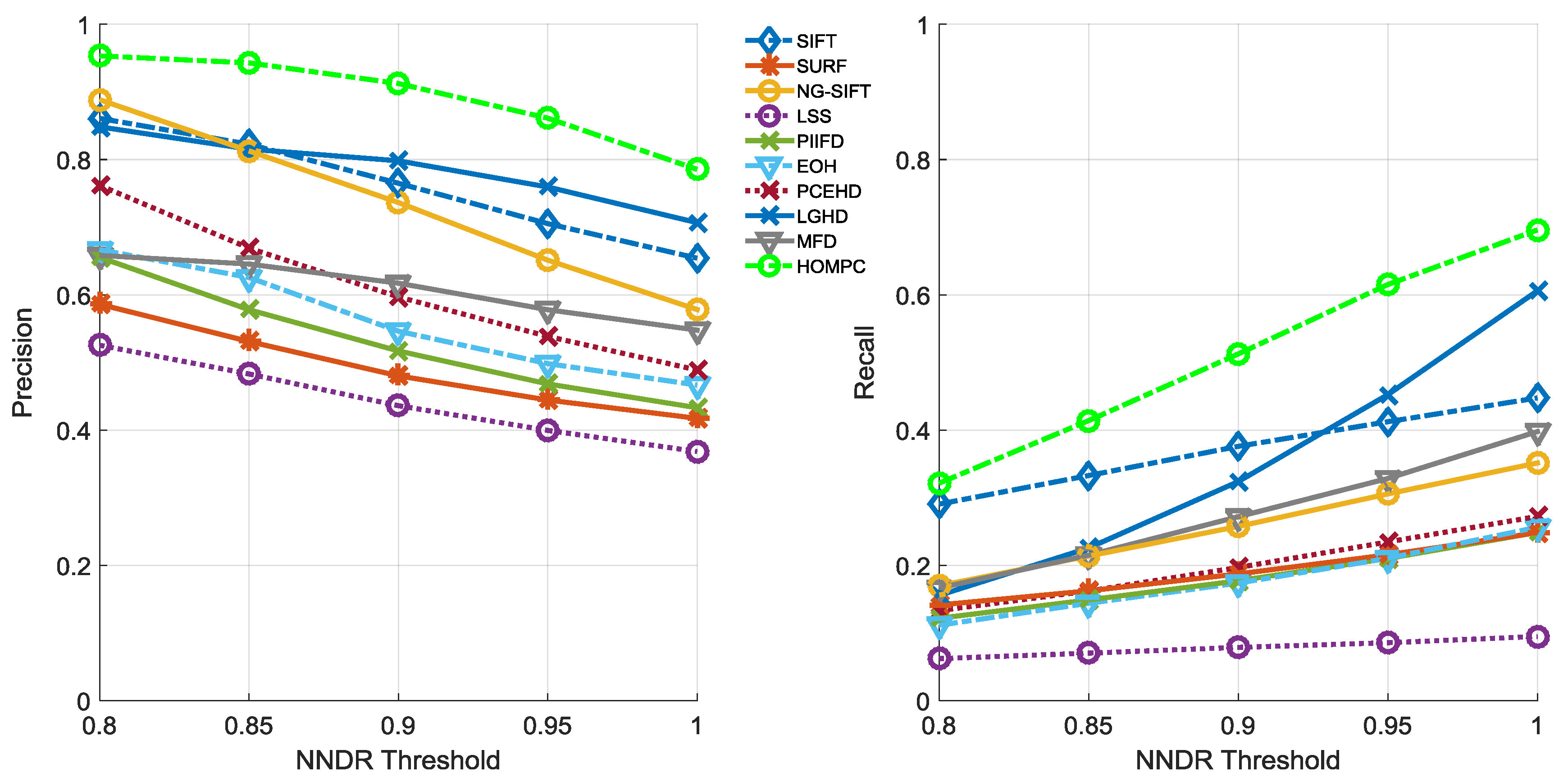
Figure 13 shows the average precision and average recall curve results obtained with the 144 pairs of visible/longwave infrared images for all the descriptors. As can be seen, on the whole, the average precision curves descend while the average recall curves ascend as the NNDR threshold increases, and the range of the precision values is much larger than that of the recall values. The average precision and recall curves of the proposed HOMPC descriptor show superior results when compared to the other descriptors. Among the other descriptors, the LGHD descriptor performs much better than the remaining descriptors, and PIIFD, EOH, PCEHD, and MFD perform better than LSS, SURF, LSS, and NG-SIFT, all of which present similar results.
The average PR curves based on the average precision and recall values and the F1-measure curves based on the precision and recall values of the 144 pairs of images for all the descriptors are provided in
Figure 14. The AUCPR results based on the average PR curves for all the descriptors are presented in
Table 5. We can clearly see that the AUCPR value of HOMPC is much greater than that of the other descriptors. Furthermore, we can see that the shape of the F1-measure curve is much more similar to that of the recall curve than the precision curve. This is because the recall and precision contribute the same weight to the F1-measure score, and the smaller recall values have more impact on the F1-measure scores. Therefore, when the NNDR threshold increases, the F1-measure curve increases at first as the recall curve also increases. Considering the comprehensive evaluation of the descriptor performance, the larger the F1-measure score, the better the performance. It is shown that the F1-measure values are the best for all the descriptors when the NNDR threshold = 1.
Figure 15 shows the correctly matched points (green lines) and falsely matched points (red lines) of two typical descriptors (SURF and LGHD) and the proposed HOMPC descriptor of sample image pair (
Figure 8a) when the NNDR threshold = 1. The correctly matched points, precision, and recall values are also displayed. Overall, we can see that the proposed HOMPC performs the best of all the descriptors.
4.3.2. Results Obtained with the UAV Dataset
Figure 16 and
Figure 17,
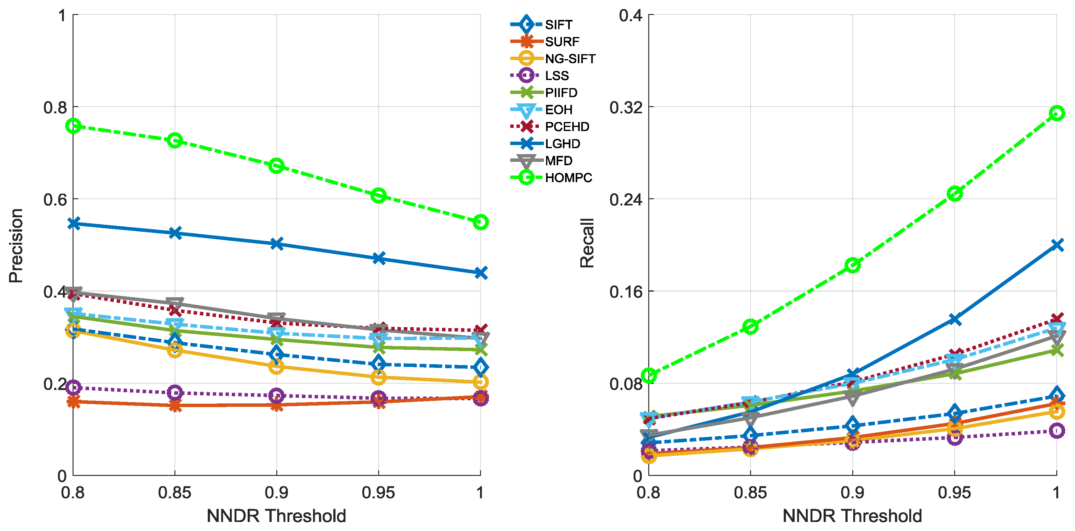
Table 6 show the average precision and recall results, as well as F1-measure and AUCPR results obtained with the 27 pairs of RGB/thermal infrared images. As can be seen in
Figure 16, the precision curves of HOMPC are again the best, but the average precision values and recall values are much lower than the average precision and recall results, as well as the F1-measure and AUCPR results for the CVC dataset, especially for the recall values. The AUCPR results of all the descriptors also indicate that the biggest value of HOMPC is just 14.95, which is much lower than most of the results for the CVC dataset. This is because the CVC dataset has been vertically rectified. In contrast, when using the low-resolution thermal infrared camera, the thermal infrared images in the UAV dataset have a lower resolution and there is noise generated in the images. Furthermore, the UAV dataset also has a slight projective transformation caused by the UAV platform. However, we can still clearly see that the proposed HOMPC descriptor is more robust than the other descriptors. Nevertheless, the AUCPR values are very low (below 15%), even if the precision of HOMPC is good when the recall is low. This means that the distances between the feature vectors for local feature regions for true or false matchings are very close but are discriminant enough when there is a need to retrieve only one region. Therefore, the threshold should be large enough to obtain more matching points.
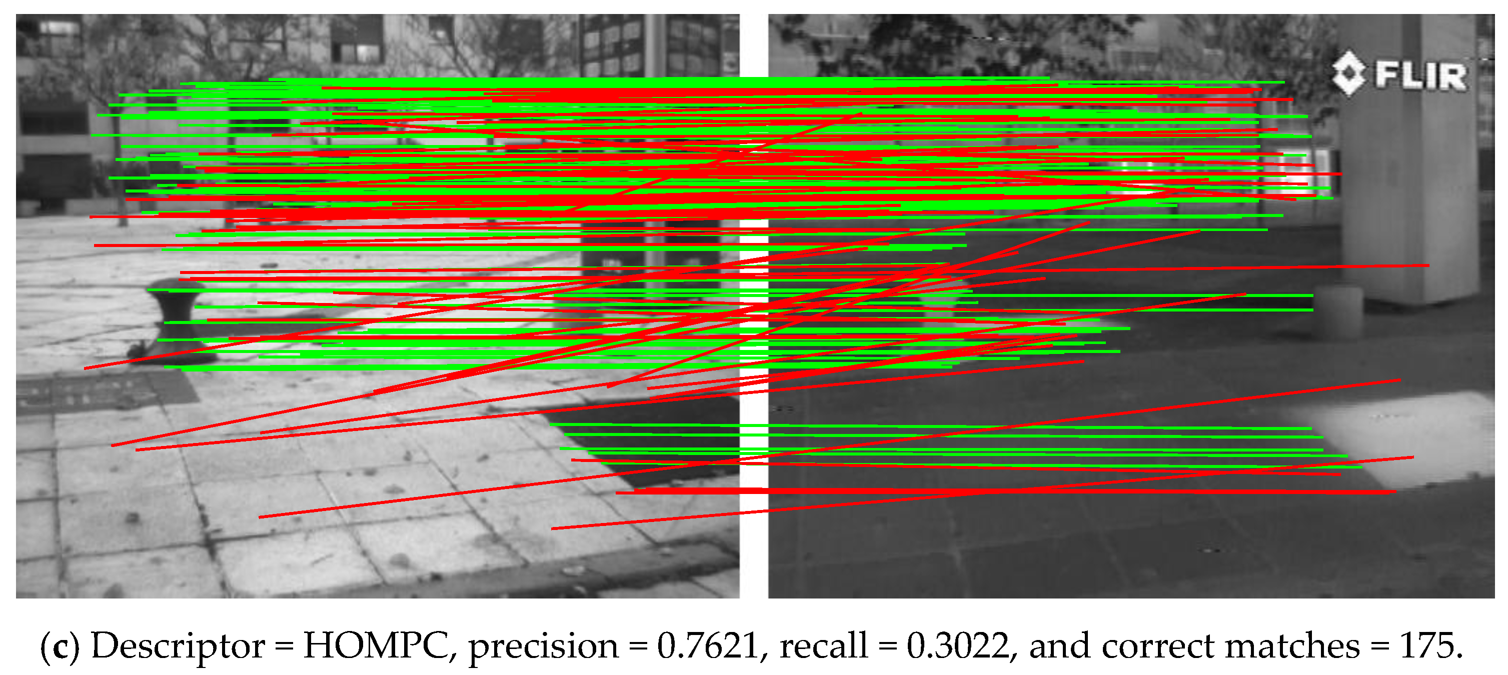
Figure 18 shows the correctly matched points (green lines) and false matches (red lines) of two typical descriptors (SURF and LGHD) and the proposed HOMPC descriptor for a pair of images (
Figure 8d) when the NNDR threshold = 1. The results of precision and recall, as well as correct matches are also given in
Figure 18a–c. It is shown that all three descriptors performed poor, but our proposed HOMPC descriptor also performed best.
4.3.3. Results Obtained with the SAT Dataset
Figure 19 and
Figure 20,
Table 7 illustrate the average precision and recall results, as well as F1-measure and AUCPR results obtained with the six pairs of multi-sensor images from the SAT dataset. Compared with the results obtained with the CVC dataset and UAV datasets, it can be seen that the average precision and recall curves for the SAT dataset are much better, as are the F1-measure curves and AUCPR values. This is because the spectral ranges of the SAT dataset are much closer than the visible and thermal infrared images of the CVC dataset and UAV dataset. The greater the spectral range, the greater the difference between two local feature regions and, hence, the less efficient the usual descriptors become. However, the proposed HOMPC descriptor performs much better than the other descriptors, and LGHD, SIFT, NG-SIFT and MFD perform better than the remaining descriptors. The results of SURF, PIIFD, EOH and PCEHD are similar, and they are much better than the results of the LSS descriptor.
Figure 21 shows the correctly matched points (green lines) and falsely matched points (red lines) of two typical descriptors (SURF and LGHD) and the proposed HOMPC descriptor of the sample image pair (
Figure 8e) when the NNDR threshold = 1. The correctly matched points, precision, and recall values are also listed. It is shown that our proposed HOMPC descriptor is suitable for the feature description of multi-temporal, multi-sensor image pairs.
4.3.4. Descriptor Computational Efficiency
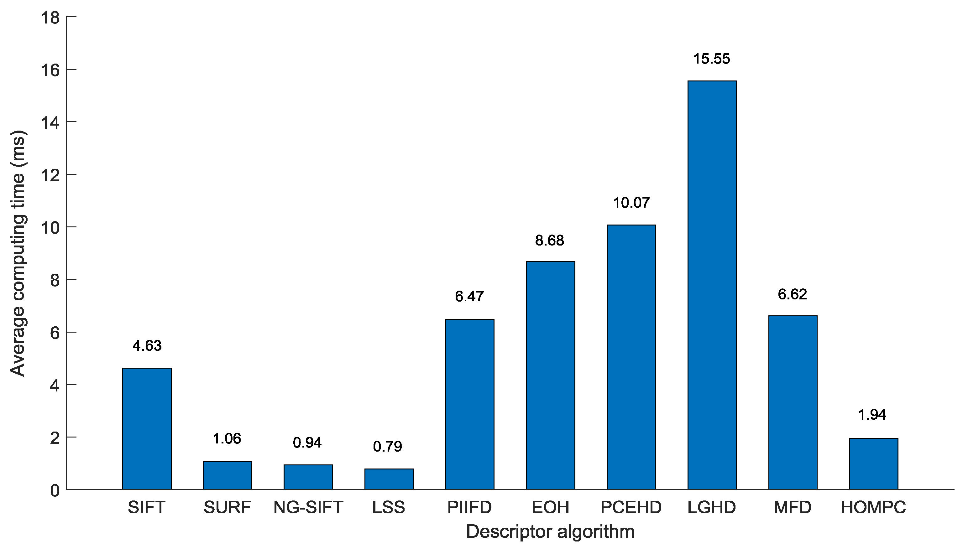
Based on the experimental results obtained using a PC with an Intel Core i3 CPU @ 2.5 GHz and 8 GB RAM, the average computation times of the descriptors for each feature point of all three datasets are shown in
Figure 22. The LGHD descriptor is associated with a high computation time. This is because the LGHD descriptor use the multi-scale and multi-oriented magnitudes of the log-Gabor filters to calculate the feature vectors of all the scales. The MFD and EOH are much faster than LGHD because they use fewer scales and filters. The PIIFD and SIFT use trilinear interpolation in the algorithm and it is, therefore, much slower than SURF, which uses Haar wavelets and integral images for image convolution to obtain a fast feature descriptor. Instead of trilinear interpolation before constructing descriptors, the NG-SIFT uses a uniform feature weighting scheme, and LSS uses the maximum self-similarity values contributes the histograms of LSS. Similarly, the proposed HOMPC uses the values of convolved PCMs and MBMs to directly contribute to the bins of each cell. In this way, it much faster to construct the HOMPC descriptor. The calculations of PCMs and MBMs based on log-Gabor filters made it slightly slower than SURF, NG-SIFT, and LSS. However, the average precision and recall results, as well as the F1-measure and AUCPR results of SURF, NG-SIFT, and LSS for the datasets performed poorly. The average computation time of the proposed HOMPC descriptor is far lower than that of the other log-Gabor-based descriptors (LGHD and MFD).
4.3.5. Influence of Rotation and Scale Variations to our Descriptor
The previous experiments have proved that the proposed HOMPC descriptor is robust to non-linear radiation variations between multi-sensor images, and the proposed HOMPC descriptor outperformed the state-of-the-art descriptors. In this part, the descriptor robustness to rotation and scale variations is evaluated, although the HOMPC descriptor is not designed to be rotationally invariant. We selected one pair of multi-temporal, multi-sensor images (
Figure 8e) as the test data.
We firstly tested the descriptor performance with rotation changes. While the left image of
Figure 8e remains unchanged, the right image of
Figure 8e is rotated from −20 to 20 degrees with an interval of five degrees. The precision, recall, and correct matches of different rotation angles are presented in
Table 8. It is shown that the rotation changes that can be tolerated are between −10 and 10 degrees. Subsequently, we tested the descriptor performance with scale variations. The left image of
Figure 8e remains unchanged, and the right image of
Figure 8e is resized from 0.5 to 1.8. It is revealed that the scale variations that can be tolerated are between 0.8 and 1.2, shown in
Table 9.
It can be observed from the results that HOMPC can tolerate rotations between images less than 10 degrees, which could be enough for multi-sensor remote sensing images, because the geometry of remote sensing images can be roughly calibrated by geographical calibration. Additionally, when dealing with the multi-sensor remote sensing images, the ground sample distance is usually known, and the images can be assigned to the same scale by resampling. Therefore, our HOMPC descriptor can tolerate scales between images from 0.8 to 1.2, which could be enough for multi-sensor remote sensing images.
4.4. Discussion
Comparing the average precision and recall results, as well as F1-measure and AUCPR results of the multi-sensor image pairs among the three datasets, we found that the results for the SAT dataset are better than for the CVC dataset and UAV dataset for all the descriptors, on the whole. This is because that the distance of the spectral range of multi-sensor devices influences the descriptor performance. In detail, the spectral modes of the SAT dataset (i.e., Band2/Band3, Pan/Pan, Pan/Band3, Band2/Band4) and the CVC dataset correspond to visible/longwave infrared, while the UAV dataset corresponds to visible/thermal infrared. Although all of the image pairs are selected from different sensors, the greater the spectral ranges of the sensors, the greater the differences between the two local feature regions are and, hence, the less efficient the local feature descriptors become. The results for the UAV dataset performed worst of all three datasets because the texture difference and the size of overlap regions affect the number of existing correct-match point pairs of the initial match point sets. The great spectral range between the visible and longwave infrared images made their texture difference become large, while the low pixel resolution of the thermal infrared camera and some geometry and perspective transformation between the visible and thermal images made the overlap regions of the reference and target images smaller. The number of existing correct-match point pairs of the initial match point sets of the UAV dataset is very limited, resulting in its low average precision and recall results, as well as the low F1-measure and AUCPR results of all descriptors.
We also found that the gradient-based descriptors, i.e., SIFT, SURF, NG-SIFT, LSS, and PIIFD are more sensitive to spectral differences than sensor differences. Meanwhile, the proposed HOMPC descriptor is more robust when dealing with greater spectral ranges, as well as different sensors. The average descriptor performance of the EOH, PCEHD, MFD, and LGHD descriptors lie between the gradient-based descriptors and the proposed HOMPC descriptor when dealing with visible and longwave infrared images. This is because the gradient-based descriptors rely on a linear relationship between images, and they are not appropriate for the significant non-linear intensity differences caused by radiometric variations.
The reason that the LGHD descriptor performs better than the gradient-based descriptors is that the LGHD descriptor use the four-scale and six-oriented log-Gabor filters (24 filters in total) to capture the multi-scale and multi-oriented magnitude feature information. The LGHD descriptor uses the distribution of the high-frequency components to express the shape and structure information of the objects and is robust to non-linear intensity variations. Since the LGHD descriptor needs to compute the feature vector at four scales, the computational efficiency is poor.
The MFD descriptor attempts to decrease the computation time of LGHD by using fewer log-Gabor filters (10 filters in total), and it shows a descriptor performance that is slightly better than LGHD when the NNDR threshold is 0.80. However, if the NNDR threshold is varied from 0.80 to 1.0 in intervals of 0.05, the descriptor performance of MFD is poorer than that of LGHD. MFD is efficient when the distances of the feature vectors between local regions of multispectral images for true or false matchings are not close, such as visible/near-infrared images. However, when the distances of the feature vectors between local regions are very close to each other, the feature vectors of local regions should be discriminant enough, as with visible/longwave infrared images. The LGHD descriptor using more log-Gabor filters than MFD can capture more feature information and is more discriminative when dealing with feature vectors between local regions that are close to each other. The average precision and recall results, as well as the F1-measure and AUCPR results obtained with the three datasets, also verify the above inference.
When using all the image pairs of the three datasets, the average results of the proposed HOMPC descriptor are much better than the other descriptors. This is because the proposed descriptor is based on the phase congruency and the distribution of the magnitude information and is robust to non-linear radiation variations of multi-sensor images. In addition, the phase congruency information ensures the precision, and the distribution of the magnitude information adds to the correct number of matched points, which is evaluated and discussed in
Section 4.2. In fact, the significant performance improvement of HOMPC over the other descriptors demonstrates the effectiveness and advantages of the proposed strategies, including the PCMs and MBMs, the novel measure for calculating the feature vector of each cell based on a convolution operation, and the dense description by overlapping blocks. We have to mention that, in order to make the proposed HOMPC descriptor more efficient, the structure and shape of the common features are captured using the overlapping blocks, in addition to the combination of magnitude and phase congruency information. It is for this reason that our descriptors are more sensitive to rotation transformations.
In addition to the advantages of average precision and recall, as well as the F1-measure and AUCPR, the computational efficiency of the proposed HOMPC descriptor is far better than that of LGHD, which can be considered the second-best descriptor when comparing the results of the multi-sensor image pairs of the three datasets. Details of the computational efficiency are provided in
Section 4.3.4. Additionally, the influences of rotation and scale variations to the proposed HOMPC descriptor is discussed in
Section 4.3.5 in detail.
Summarizing the quantitative experimental results described in
Section 4.3 and
Section 4.4, we can draw the following summaries:
The proposed HOMPC descriptor is designed for the description problem of multi-sensor images with non-linear radiation variations.
In the experiments undertaken in this study, HOMPC achieved very good average precision and recall on the three datasets.
The descriptor performance of HOMPC is far superior to that of the classical local feature descriptors to describe the local regions of multi-sensor images.
The time consumption of HOMPC is far lower than that of the other log-Gabor-based descriptors (LGHD and MFD).
The proposed HOMPC descriptor can tolerate small amounts of rotation and scale variations.
5. Conclusions
In this paper, we proposed a novel descriptor (named HOMPC) based on the combination of magnitude and phase congruency information to capture the common information of multi-sensor images with non-linear radiation variations. We first introduce the concept of magnitudes of log-Gabor filters, and we then propose the PCMs and MBMs, preparing for the convolution operation. To accelerate the computational efficiency of each feature vector, we apply Gaussian filters and mean filters to the PCMs and MBMs, respectively. To capture the structure and shape properties of local regions, we describe the local regions using the HPC and HOM based on a dense grid of local histograms. Finally, we combine the HOM and HPC to obtain the proposed HOMPC descriptor, which can capture more common features of multi-sensor images from the combination of magnitude and phase congruency information.
To make a fair comparison between the local feature descriptors, we used the same feature detection method and the same similarity metric to uniformly test the descriptor performance in the experiments. In the experiments, we first studied the parameters and tested the advantages of integrating the HOM and HPC. The HOMPC descriptor was then evaluated using three datasets (CVC dataset, UAV dataset, and SAT dataset) and compared to the state-of-the-art local feature descriptors of SIFT, SURF, NG-SIFT, LSS, PIIFD, EOH, PCEHD, LGHD, and MFD. The experimental results confirmed that HOMPC outperforms the other local feature descriptors. Moreover, by designing a fast method of constructing the feature vectors for each block, HOMPC has a much lower run time than LGHD, which achieved the second-highest F1-measure and AUCPR values in the experiments. Finally, the rotation and scale variations to the proposed HOMPC descriptor are evaluated and the results show that our HOMPC descriptor tolerates small amounts of rotation and scale variations, although the purpose is to address the non-linear radiation variations between multi-sensor images.
The HOMPC descriptor can be applied to change detection, target recognition, image analysis, image registration, and fusion of multi-sensor images. In our future work, we will test our HOMPC descriptor on more multi-sensor images with non-linear radiation variations, such as optical and SAR images, and optical and LiDAR images.


