Four-Stage Inversion Algorithm for Forest Height Estimation Using Repeat Pass Polarimetric SAR Interferometry Data

Abstract

This paper proposes a new method for forest height estimation using single-baseline single frequency polarimetric synthetic aperture radar interferometry (PolInSAR) data. The new algorithm estimates the forest height based on the random volume over the ground with a volume temporal decorrelation (RVoG+VTD) model. We approach the problem using a four-stage geometrical method without the need for any prior information. In order to decrease the number of unknown parameters in the RVoG+VTD model, the mean extinction coefficient is estimated in an independent procedure. In this respect, the suggested algorithm estimates the mean extinction coefficient as a function of a geometrical index based on the signal penetration in the volume layer. As a result, the proposed four-stage algorithm can be used for forest height estimation using the repeat pass PolInSAR data, affected by temporal decorrelation, without the need for any auxiliary data. The suggested algorithm was applied to the PolInSAR data of the European Space Agency (ESA), BioSAR 2007 campaign. For the performance analysis of the proposed approach, repeat pass experimental SAR (ESAR) L-band data, acquired over the Remningstorp test site in Southern Sweden, is employed. The experimental result shows that the four-stage method estimates the volume height with an average root mean square error (RMSE) of 2.47 m against LiDAR heights. It presents a significant improvement of forest height accuracy, i.e., 5.42 m, compared to the three-stage method result, which ignores the temporal decorrelation effect.

1. Introduction

Forest height is an important parameter in quantitative analysis of the carbon cycle at regional and global scales. Radar imagery provides us a great promise for the forest height estimation because of its global coverage and low weather sensitivity [1]. In recent years, the PolInSAR technique has been developed in terms of forest characterization based on the coherent combination of radar polarimetry and SAR interferometry technologies [2]. The capability of the PolInSAR technique results from its sensitivity to the 3-D distribution of scatterers in the vertical direction to separate the volumetric and surface scattering phase centers [3,4]. In the ideal case, the forest height can be estimated by scaling the phase difference between two interferograms corresponding to the volume-only and ground-dominant polarization states [3]. However, the phase centers of two selected polarization states depend on the propagation properties, such as wave extinction and the vertical structure of the canopy. In this regard, a physical model has been developed to invert the PolInSAR measurement into the forest height, taking into account the effective parameters of the wave and forest [5]. The random volume over ground (RVoG) model is a simple physical model, which considers both the volume layer and ground interactions. Accordingly, the vegetation layer is modeled as a homogeneous volume constituted by randomly-oriented particles by a constant wave attenuation in the media over a non-penetration ground [5]. The RVoG model addresses the complex coherence in each polarization state as a function of the volume thickness, the ground underlying phase, the mean extinction coefficient, and the surface-to-volume backscattering ratio. Thus far, different methods have been proposed to estimate the forest height based on the RVoG model. In this respect, a six-dimensional nonlinear optimization method was suggested using an iterative procedure [5]. According to the nonlinear nature of the problem, the most important disadvantage of this optimization method is that the results are often sensitive to the initial values of the variables. In order to overcome the above-mentioned disadvantages, a simple geometrical three-stage method was also proposed [4]. This method can estimate the ground phase, the forest height and the mean extinction coefficient without the need for a priori information and a time consuming iterative procedure. In this framework, this algorithm has been widely used in forest height estimation using the RVoG model due to its simplicity and time savings [6,7,8,9]. Basically, the RVoG model does not account for dynamic changes within the scene occurring in repeat pass PolInSAR data. For the purpose of the temporal decorrelation compensation, a two-layer model, random volume over ground with volume temporal decorrelation was applied [10]. The RVoG+VTD model incorporates the temporal decorrelation effect in the RVoG scattering model only in a very abstract way. Although the three-stage method can be applied for the inversion of the RVOG+VTD model, the accuracy of the inversion results depends on how well the extinction value is determined from an auxiliary data [10,11]. In reality, the RVoG+VTD model can be inverted using the three-stage method by fixing the mean extinction coefficient to a predefined value. In this framework, the accuracy of the estimated forest height depends on the particular value chosen for the mean extinction coefficient. In order to deal with this issue, a multi-baseline PolInSAR data was employed to invert the RVoG+VTD model without the need for an axillary data [12,13]. Since temporal decorrelation is one of the most common decorrelation resources over the vegetated land surface, a random motion over ground model (RMoG) has been developed to compensate for the temporal decorrelation in the coherence model. The RMoG model addresses the dynamic changes as a random motion of the scatterers with standard deviation that varies linearly along the vertical direction in the canopy [11,14]. In this framework, the RMoG model is characterized by two additional parameters, namely the canopy and ground motion standard deviation. In practice, the obtained solution depends on the initial values of the unknown parameters, strongly. Therefore, due to the nonlinear nature of the model, poor starting values lead to an inaccurate estimation [11]. In order to alleviate this problem, a supervised algorithm was proposed to invert the RMoG model to solve all unknown parameters [15]. It should be noted that, by tweaking the mean extinction coefficient value in the RVoG+VTD model, we are able to achieve an estimation performance similar to the ones of the RMoG result [11].

This research addresses the temporal decorrelation effect in the repeat pass PolInSAR data processing as a critical problem in the forest height estimation based on the RVoG+VTD model. As already noticed, in the absence of the predefined value for the volume temporal decorrelation or the mean extinction coefficient, the three-stage method is inefficient for the RVoG+VTD inversion. In this framework, we propose a new geometrical method for the RVoG+VTD retrieval using single-baseline PolInSAR data without the need for any auxiliary data, prior information or initial values of the variables. Hence, the advantage of the suggested method, which is termed four-stage algorithm, is the mean extinction coefficient estimation, independently. In other words, the proposed algorithm is used to overcome the limitation of the three-stage method in the RVoG+VTD inversion due to its capability of the biophysical parameters and temporal decorrelation coefficient estimation, geometrically.

The structure of this paper is as follows: In Section 2, the selected PolInSAR dataset and the test site are introduced. Additionally, the RVoG model, three-stage inversion method, and the RVoG+VTD model are reviewed as the general underlying theory. Then, the proposed four-stage inversion algorithm is discussed. In Section 3, the results of the proposed method are analyzed by comparing the three-stage results against LiDAR heights. Finally, the research findings and their implications are discussed in Section 4 and the advantages and limitations of the proposed four-stage algorithm are discussed in Section 5.

2. Materials and Methods

In this section the selected PolInSAR dataset and the test site are introduced. Additionally, the underlying theory of the RVoG model, the conventional three-stage method, the RVoG+VTD model, and the proposed four-stage method are discussed.

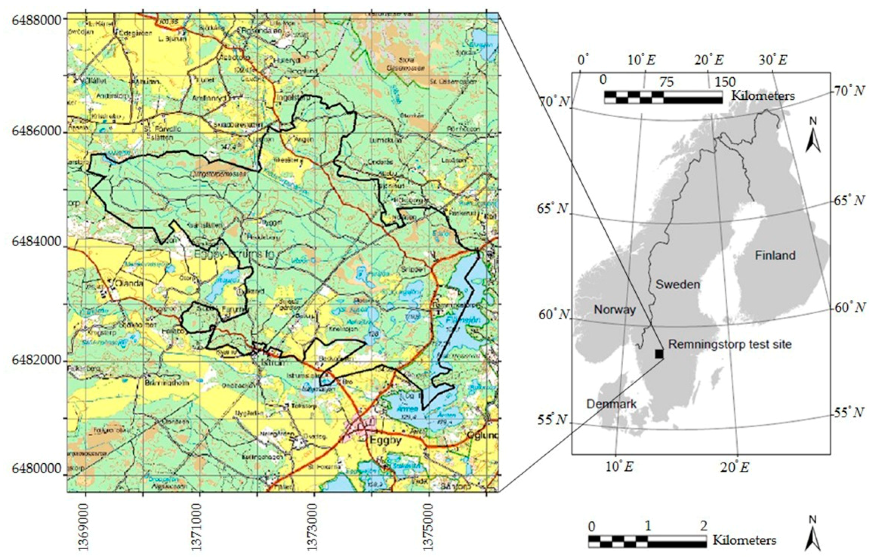
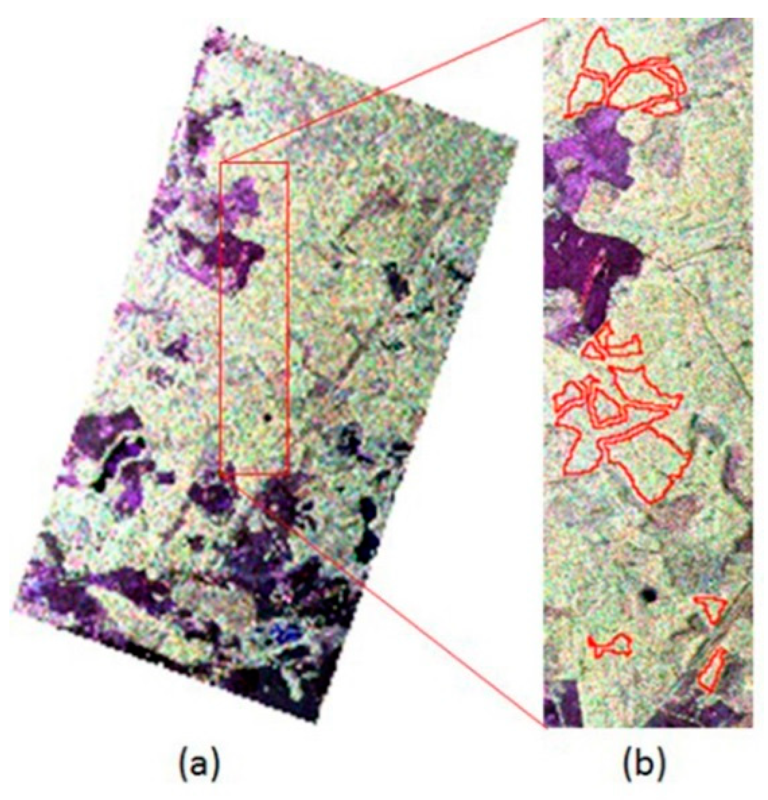
2.1. Test Site and PolInSAR Data Set Description

A pair of fully polarimetric L-band airborne data from the BioSAR 2007 ESA campaign are employed to validate the result of the suggested inversion algorithm. The utilized PolInSAR data have been collected from the Remningstorp test site (58°28′N, 13°38′E) in Southern Sweden, as shown in Figure 1 [16].

About 1200 ha in the test site have been covered by productive forest in a fairly flat landscape in a way that its height varies between 120 and 145 m above the mean sea level. The selected L-band data pair have been acquired with 8 m spatial baseline and resolution of 0.74 m in range and 1.5 m in azimuth direction. Two images have been acquired on 31 March 2007 and 2 May 2007 with more than one month temporal baseline. In the following, LiDAR measurements with resolution of 0.5 m are used as reference height to evaluate the results. All processing has been applied to a part of the image consists of 15 particular stands. The delineation of the used forest stands has been presented in Figure 2.

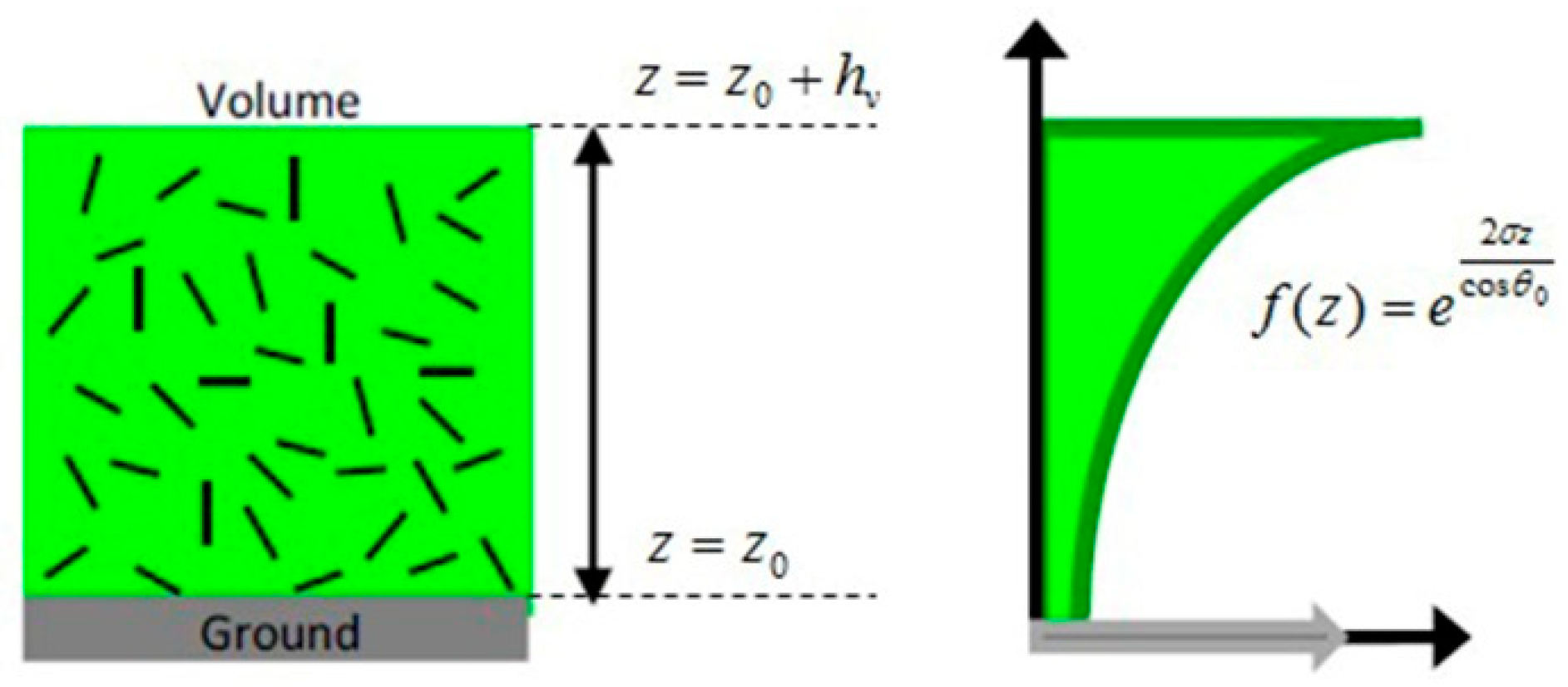
2.2. Random Volume over Ground Model

Random volume over ground is a simple physical model to interpret the forest structure information by making use of the complex coherence in different polarization states [5,17]. Figure 3, is a schematic representation of physical interpretation of the RVoG model. As shown in Figure 3, the RVoG model uses an exponential structure function as [1]:

$$f(z)=e^{\frac{2\sigma z}{\cos {\theta }_0}},$$

(1)

wherein σ is the constant mean extinction coefficient and θ₀ is incidence angle.

According to the no ground decorrelation assumption, the complex coherence in a specific polarization state is expressed as [5]:

$$\gamma (\underset{\_}{w})=e^{i{\phi }_0}\frac{{\gamma }_v+\mu (\underset{\_}{w})}{1+\mu (\underset{\_}{w})},$$

(2)

in which $\gamma (\underset{\_}{w})$ represents the interferometric coherence in a specific polarization state, $e^{i{\phi }_0}$ is the ground complex coherence, ${\gamma }_v$ refers to the complex volume coherence, and $\mu \left(\underset{\_}{w}\right)$ is the effective ground-to-volume backscattering ratio which is the only polarization dependent parameter in Equation (2). By isolating the polarization dependent parameter in a single term, Equation (2) can be rewritten as [5]:

$$\gamma (\underset{\_}{w})=e^{i{\phi }_0}\left({\gamma }_v+L(\underset{\_}{w})(1-{\gamma }_v)\right),L(\underset{\_}{w})=\frac{\mu (\underset{\_}{w})}{1+\mu (\underset{\_}{w})}$$

(3)

where $L(\underset{\_}{w})$ lies in the range $0\le L(\underset{\_}{w})\le 1$, with limits occurring at one end for pure volume scattering ($\mu \left({\underset{\_}{w}}_v\right)=0$) and at the other for pure surface polarization state ($\mu \left({\underset{\_}{w}}_s\right)=\infty$). According to Equation (3), the coherence values in different polarization states lie along a straight line. The volume-only coherence is also given explicitly as a function of the constant mean extinction coefficient and the forest height, $h_v$ as follows [5]:

$${\gamma }_v=\frac{2\sigma }{\cos {\theta }_0(e^{\frac{2\sigma h_v}{\cos {\theta }_0}}-1)}{\displaystyle {\int }_0^{h_v}{e}^{i{k}_{z}z}{e}^{\frac{2\sigma z}{\cos {\theta }_0}}dz}$$

(4)

where $k_z$ represents the vertical wave number which can characterized as [1]:

$$k_z=\frac{4\pi B_{\perp }}{\lambda R\sin {\theta }_0}$$

(5)

wherein $B_{\perp }$ is the perpendicular spatial baseline, $\lambda$ is the signal wave length, and $R$ is the slant range. Equations (3) and (4) show a nonlinear relation between four unknown parameters (i.e., $h_v$, $\sigma$, ${\phi }_0$ and $\mu (w)$); in the RVoG model.

As discussed in Section 1, several methods have been developed for forest height inversion based on the RVoG model, such as DEM differencing [3], the six-dimensional nonlinear optimization method [5], and the three-stage method [4]. The three-stage algorithm has been widely used in forest height estimation due to its simplicity and time saving [6,7,8]. In this framework, we used the three-stage method as our basis algorithm.

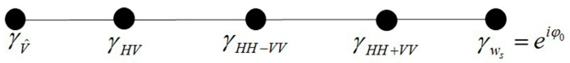
2.3. Three-Stage Inversion Method

In the last two decades several model based forest height inversion methods have been suggested using the single-baseline PolInSAR configuration [3,4,11,19]. Among these methods the three-stage algorithm is a geometrical straightforward approach without the need for auxiliary data. In this respect, the three-stage algorithm has been one of the most frequently used method in single or dual baseline inversion method [6,7,8,20]. The above-mentioned method breaks the inversion procedure down into three separate steps, least squares line fit, ground phase estimation and, finally, the canopy height and the mean extinction coefficient estimation.

Based on the RVoG model, the coherence signature in a specific resolution cell, which contains only two different phase centers, is a straight line in the complex unit circle [21]. In this respect, the first step of the three-stage method is the coherence line fitting using the complex coherence value in Pauli basis. Thereafter, the fitted line can be used to secure the intersection points between the coherence line and the complex unit circle (CUC) as the ground coherence candidates. In other words, according to the no ground decorrelation assumption in the RVoG model, two intersection points between CUC and the coherence line are the ground coherence candidates with $\left|{\lambda }_g\right|=1$, as shown in Figure 4. The main purpose of the second step is to choose the ground coherence between two candidates. Based upon the scattering physics, a strong scattering contribution from the ground is present in the direct or dihedral ground backscattering, while the canopy scattering has a strong HV signal [4,22]. In this regards, it is very unlikely that the weakest ground to volume scattering ratio will arise in the HV channel. Hence, it is reasonable to expect that the ground coherence will be ranked furthest away in distance from the HV coherence along the coherence line as shown in Figure 5. Finally, in the third step, two remained unknown parameters (i.e., $h_v$ and $\sigma$); are estimated according to the Equation (4). For the purpose of using Equation (4), an observed polarization state is employed as the volume only channel. In doing so, the three-stage algorithm selects the observed volume only coherence among the common polarization states, such as HH, VV, HH-VV, HH+VV, and HV. Although Equation (4) provides two separate equations based on the observed volume only coherence, the non-linear nature of the problem leads to the need for the initial values of the $h_v$ and $\sigma$. In order to alleviate this problem, the three-stage method proposed a geometrical solution to estimate the correspondence volume height and the mean extinction coefficient. Figure 4 depicts the volume coherence loci for two constant mean extinction coefficient values using Equation (4). The coherence curves and the coherence line intersection points are the calculated volume only coherence candidates which are employed to pre-calculate a look up table (LUT), as a function of the $h_v$ and $\sigma$. It is worth stressing that, the three-stage method assumes ${\gamma }_{HV}$ is the observed volume only coherence which has the upper phase center among the common polarization states. Since the intersection point corresponding to ${\gamma }_v(h_v,\sigma ={\sigma }_1)$ generates a negative $\mu$ in the observed volume coherence, it cannot be a physical solution. In this regard, all intersection points on the ambiguous line segment are used to pre-calculate the LUT. Finally, the estimation of the volume height and the mean extinction coefficient can be secured by comparing the calculated volume coherences and the observed volume coherence. In this respect, the volume height and the mean extinction coefficient, which minimize the distance between the calculated coherence and the observed volume coherence are the inversion-solution couple.

2.4. Random Volume over Ground with Volume Temporal Decorrelation

The temporal decorrelation is a major source of decorrelation in the repeat pass interferometry which limits the interferometric capabilities of data. In general, the dynamic changes caused by wind and other changes such as vegetation growth, seasonal variation and manmade changes can severely affect the coherence measurements. Consequently, the repeat pass PolInSAR retrieval requires modelling the temporal decorrelation effect. Since the RVoG model does not take the temporal decorrelation effect into account, the estimated volume height is fairly overestimated due to the temporal decorrelation effect. To cope with this limitation, two complementary models were suggested, i.e., RVoG+VTD [10] and RMoG [11,14] models. As discussed in Section 1, Papathanassiou and Cloude have suggested a supervised three-stage method to invert the RVoG+VTD model [10] and Lavalle and Hensley have proposed an eight dimensional nonlinear optimization method for RMoG model inversion [11]. In this paper, we addressed the temporal decorrelation based on the RVoG+VTD model.

To compensate the temporal decorrelation effect in the RVoG model, two real multiplying factors were added to the RVoG model as [10]:

$$\gamma {(\underset{\_}{w})}^{td}=e^{i{\phi }_0}\frac{\left|{\gamma }_{tv}\right|{\gamma }_v+\left|{\gamma }_{tg}\right|\mu (\underset{\_}{w})}{1+\mu (\underset{\_}{w})}$$

(6)

where $\left|{\gamma }_{tv}\right|$ and $\left|{\gamma }_{tg}\right|$ are the temporal decorrelation coefficients of volume and ground coherences, respectively, both ranging from zero to one and $\gamma {(\underset{\_}{w})}^{td}$ is the complex coherence in a desired polarization state taking the temporal decorrelation into account. Generally, the most common temporal decorrelation effect comes from the wind-induced movement of the canopy layer within a few-day temporal baseline [23]. With such an argument, the scattering properties of the ground is assumed constant during the time, i.e., $\left|{\gamma }_{tg}\right|=1$. In this respect, Equation (6) can be simplified with only the volume temporal decorrelation multiplying factor (i.e., RVoG model with volume temporal decorrelation, RVoG+VTD) as [10]:

$$\gamma {(\underset{\_}{w})}^{td}=e^{i{\phi }_0}\frac{\left|{\gamma }_{tv}\right|{\gamma }_v+\mu (\underset{\_}{w})}{1+\mu (\underset{\_}{w})}$$

(7)

where ${\gamma }_v$ is characterized as Equation (4). Furthermore, Equation (7) can be rewritten as:

$$\gamma {(\underset{\_}{w})}^{td}=e^{i{\phi }_0}\left(\left|{\gamma }_{tv}\right|{\gamma }_v+L(\underset{\_}{w})(1-\left|{\gamma }_{tv}\right|{\gamma }_v)\right),L(\underset{\_}{w})=\frac{\mu (\underset{\_}{w})}{1+\mu (\underset{\_}{w})}$$

(8)

Based upon Equation (8), the $\left|{\gamma }_{tv}\right|$ leads to a degradation of the amplitude of the volume coherence and it does not affect the interferometric phase center [10,15]. Additionally, Equation (8) shows that the coherence loci in the complex plane is a straight line. The coherence lines correspond to the RVoG and the RVoG+VTD models are depicted in Figure 6 as the blue line and dotted blue line respectively. As shown in Figure 6, the temporal decorrelation reduces the coherence amplitude in all polarization states. In this framework, the volume-only coherence point moves radially towards the origin because of the temporal decorrelation effect. In other words, by varying $\left|{\gamma }_{tv}\right|$ the coherence line is rotated about the ground coherence point. In the extreme case, $\left|{\gamma }_{tv}\right|=0$, the volume coherence fall into the origin of the CUC and in the other extreme case of no temporal decorrelation the RVoG+VTD model conforms to the RVoG model.

In order to invert the RVoG+VTD model, the ground phase can be estimated by implementing the first two stages of the conventional three-stage method. However, the amplitude of the observed volume coherence corresponds to the product of the amplitude of the pure volume only coherence, $\left|{\gamma }_v\right|$, and $\left|{\gamma }_{tv}\right|$. Hence, the observed volume coherence should be shifted radially towards the top to compensate the temporal decorrelation effect. In other words, as there is no knowledge about the volume temporal decorrelation value, $\left|{\gamma }_{tv}\right|$, the radius segment beyond $\left|{\gamma }_{tv}\right|{\gamma }_v$ up to the complex unit circle is the corresponding ambiguous line segment of the volume-only coherence. Accordingly, the forest height estimation, based on the RVoG+VTD model using single-baseline PolInSAR data, is insoluble without the information about the mean extinction or volume temporal decorrelation value. In order to overcome this challenge, employing a fixed mean extinction coefficient is suggested [10]. As shown in Figure 7, the volume-only coherence point can be found as the intersection point between the fixed extinction volume coherence curve and the constant volume coherence phase line, i.e., $\phi ={\phi }_{HV}$. Finally, the forest height and the volume temporal decorrelation corresponding to the calculated volume only coherence are the inversion-solution couple. In practice, the accuracy of the estimated height depends on the selected constant mean extinction value. In other words, the results are changeable by tweaking the mean extinction value. This makes the RVoG+VTD inversion with a single-baseline PolInSAR configuration a challenge [11]. Alternatively, the RVoG+VTD can be inverted using a dual baseline inversion algorithm [12].

2.5. Four-Stage Inversion Method

As already noticed, the three-stage method is not able to estimate the biophysical parameters and the volume temporal decorrelation multiplying factor in the RVoG+VTD model. In order to overcome this issue, Papathanassiou and Cloude proposed to use a fixed mean extinction coefficient and then to estimate the two remaining variables (i.e., the forest height and the real valued volume temporal decorrelation); geometrically [10]. Intuitively, the accuracy of the results depends on how good the guess is for the mean extinction coefficient value. In order to alleviate this problem, we propose a four-stage algorithm which estimates the reliable mean extinction coefficient in the third stage and finally estimates the forest height and the real valued volume temporal decorrelation multiplying factor in the last stage. In other words, the four-stage algorithm extends the three-stage procedure to invert the RVoG+VTD model. As shown in Figure 6, the volume temporal decorrelation, doesn’t affect the coherence locus. Therefore, first two steps of the proposed method is carried out similar to the conventional three-stage algorithm in order to estimate the ground underlying phase.

In general, the mean extinction coefficient is a function of the forest biophysical properties such as volume height and forest density and the sensor parameters such as wave frequency. The higher mean extinction, which is took place at higher frequencies, leads to an effective backscattering from the top of the canopy [24]. Based on this, the mean extinction coefficient value and the penetration depth are inversely related. Also, the volume decorrelation increases with the penetration depth. Therefore, the volume coherence amplitude and the penetration depth are indirectly related. Figure 8 represents the complex volume coherence variation inside the CUC for varying extinction coefficients when k_z = 0.1567 and θ₀ = 45°. A look at Figure 8 reveals that the coherence loci fall in to the trigonometric circle origin owing to the extinction coefficient reduction. On the other hand, the volume scattering phase center moves towards the top of the canopy according to the higher mean extinction value, which corresponds to the low penetration depth. Consequently, the mean extinction coefficient and the complex volume coherence are significantly related to each other.

With such an argument, Managhebi et al. proposed to employ the relative location of the observed volume coherence on the coherence line to limit the range of the mean extinction coefficient in an improved three-stage method [7]. In this framework, a geometrical index was suggested to interpret the relative location of the observed volume coherence, γ_HV, on the coherence line as [7]:

$$D.I=\frac{A.L}{V.L}$$

(9)

wherein $D.I$ is the distance ratio index, $A.L$ and $V.L$ are the ambiguous line length and the visible line length respectively, as shown in Figure 9. In this geometrical index, the $A.L$ has been normalized by the $V.L$ to generalize the index. The geometrical index is a real non-negative value with limits occurring at one end for the case of no penetration ($D.I=0$) and at the other by pure surface scattering ($D.I=\infty$) when the penetration depth is equal to the volume height theoretically. Figure 10 depicts the mean extinction value calculated by the three-stage method in 75 pixels of three simulated PolInSAR data $\left(h_v=20\mathrm{m}\right)$ for three species (i.e., deciduous and two types of pine); versus D.I. As expected, the mean extinction value and D.I value are inversely related. As shown in Figure 10, the geometrical index can be further utilized for mean extinction coefficient estimation effectively. Therefore, in this research, we defined the mean extinction coefficient as the following linear function of the distance ratio index as:

$$\sigma =aD.I+b$$

(10)

where $\sigma$ is the mean extinction coefficient, $D.I$ is the distance ratio index, $a$ and $b$ are the model parameters. To compute the variables of the linear model we used a real L-band PolInSAR data pair. Figure 11 represents the flowchart for estimating the unknown parameters of Equation (10) using the least squares method.

In summary, the following step-by-step outline describes finding the linear model parameters, $a$ and $b$.

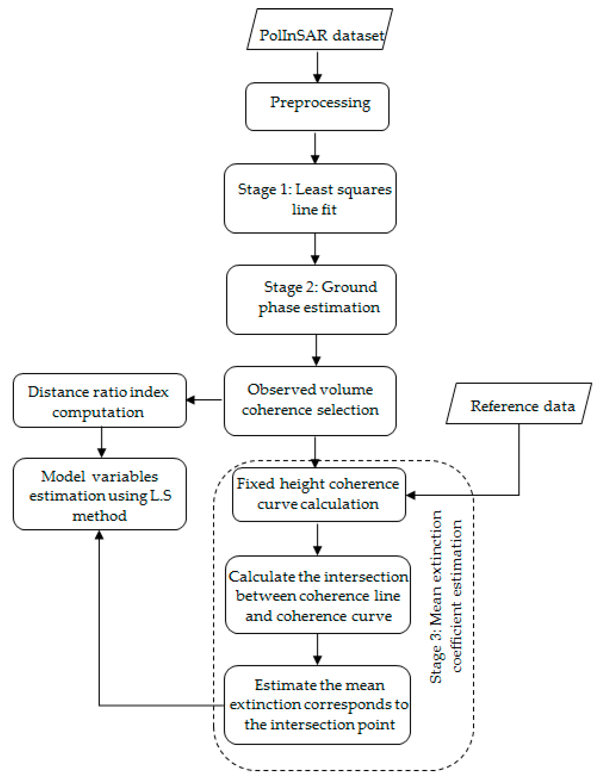
• Fit the least square line on the Pauli basis coherences and find the intersection points between the fitted line and the CUC as the ground coherence candidates.
• Choose the ground underlying phase between two candidates.
• Extract the forest height from LiDAR measurement as the reference height.
• Calculate the D.I for the selected pixels using Equation (9).
• Calculate the fixed height coherence locus for all selected pixels using Equation (4).
• Estimate the mean extinction coefficient corresponding to the intersection point between the volume coherence locus and the coherence line for all selected pixels.
• Calculate the model parameters using the least square method based on Equation (10).

Afterwards, Equation (10) is employed in the third stage of the four-stage algorithm to compute the mean extinction coefficient in each pixel. Figure 12 shows the flowchart of the four-stage algorithm for forest height estimation based on the RVoG+VTD model.

As illustrated in Figure 12, the first two steps of the proposed four-stage inversion method are carried out similar to the conventional three-stage algorithm to estimate the ground underlying phase. The main difference between the proposed method and the conventional three-stage algorithm lies in the mean extinction coefficient estimation. As discussed in Section 2.4, the three-stage algorithm uses a fixed mean extinction coefficient to reduce the number of the variables in the RVoG+VTD model. This is while the four-stage method calculates the mean extinction coefficient based on the signal penetration and the relative location of the volume coherence on the coherence line. Equation (10) is the general model which determines the mean extinction coefficient as a linear function of the distance ratio index in the third stage of the suggested method. As discussed in Section 2.4, the volume temporal decorrelation reduces the coherence amplitude in all polarization states but it does not affect the coherence phase at all. As a result, the radius segment beyond $\left|{\gamma }_{tv}\right|{\gamma }_v$ up to the CUC is the ${\gamma }_v$ ambiguous line segment as shown in Figure 13 by the dotted red line. Accordingly, the corrected observed volume only coherence is on the ambiguous line segment of the observed volume coherence. Furthermore, the fixed mean extinction curve is the volume coherence locus. Therefore, the intersection point between the volume coherence curve and $\phi ={\phi }_v$ is selected as the corrected observed volume coherence and the corresponding volume height and the volume temporal decorrelation are the four-stage solution couple.

In summary, the proposed four-stage method follows the following four steps.

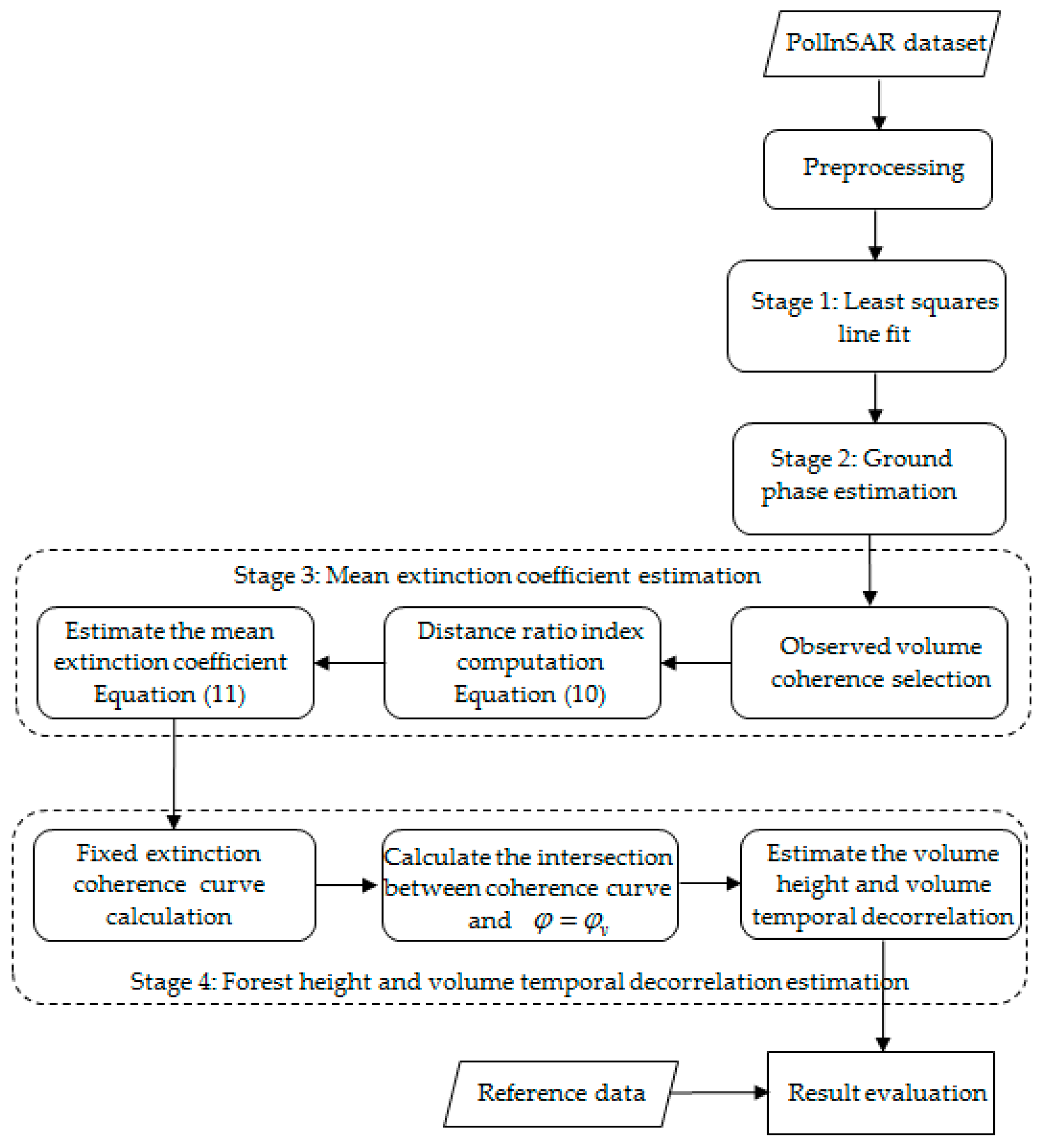
• Fit the least square line on the Pauli basis coherences and find its intersections with CUC as the ground coherence candidates.
• Choose the ground coherence between two candidates according to the surface to volume backscattering ratio.
• Calculate the D.I using Equation (9) and estimate the mean extinction coefficient using Equation (10).
• Find the fixed mean extinction coherence locus using Equation (4) and estimate the volume height and the real temporal decorrelation multiplying factor from the intersection point between the volume coherence loci and $\phi ={\phi }_v$.

3. Results

The coregistered SAR image pair was used to generate the coherency matrix using PolSARpro version 5.1 (https://earth.esa.int/web/polsarpro/home). First, the flat earth phase removal step was applied and then coherency matrices were calculated using an 11 × 11 boxcar filter. Figure 14 depicts the efficiency of the proposed four-stage algorithm in the volume thickness estimation, in comparison with the three-stage method for a pixel. The volume height has been estimated in a single pixel, with a height of 20.02 m, based on the RVoG and RVoG+VTD model using three-stage and four-stage algorithms respectively. As already noticed, the first two steps of the mentioned methods are the same. Therefore, the ground underlying phase has been estimated based on the first two stages of the three-stage method. The last two parameters of the RVoG model (i.e., volume height and the mean extinction coefficient); can be estimated at the final stage of the conventional three-stage method. According to Equation (4), the volume height and the mean extinction coefficient corresponding to the observed volume coherence are the RVoG solution. Figure 14 depicts all fixed extinction coherence curves corresponding to the mean extinction coefficient varied between 0 to 0.9 dB/m. The calculated volume coherence candidates are determined according to the fixed extinction coherence loci and the fitted coherence line intersection points, as shown in

Table 1. Look-up table.

Distance Value in CUC between γv and γHV	Mean Extinction Coefficient	Estimated Forest Height
0.0062	0	30
0.1706	0.1	26
0.2574	0.2	23
0.3069	0.3	21
0.3371	0.4	21
0.3578	0.5	21
0.3677	0.6	22
0.3763	0.7	22
0.3835	0.8	22
0.3861	0.9	23

. Finally, the calculated volume coherence can be chosen based on the shortest distance from the observed volume coherence. As shown in Figure 14, the fixed mean extinction coherence locus corresponding to ${\gamma }_v\left(h_v,\sigma =0\mathrm{dB}/\mathrm{m}\right)$ is the nearest curve to the ${\gamma }_v$. However, this is not physically possible as it generates negative $\mu$ in the ${\gamma }_v$. As a result, ${\gamma }_v\left(h_v,\sigma =0.1\mathrm{dB}/\mathrm{m}\right)$ is the selected fixed mean extinction coherence locus in the conventional three-stage method and the corresponding volume height is 26 m. As expected, the volume height is overestimated by using the RVoG model because this model interprets the temporal decorrelation as the volumetric decorrelation. A look at Table 1 reveals that the mean extinction coefficient is an important and decisive parameter in the three-stage method. Hence, the RVoG+VTD inversion using the three-stage method depends on how good the guess is for the mean extinction coefficient value. Therefore, due to the lack of information about the mean extinction value, the three-stage method is not able to invert the RVoG+VTD model.

In this respect, the proposed four-stage method is used for forest height estimation based on the RVoG+VTD model. As discussed in Section 2.5, the mean extinction coefficient is estimated in the third stage of the four-stage algorithm using Equations (9) and (10). As illustrated in Figure 14, the A.L and V.L are obtained as 0.5175 and 1.2545 for the selected pixel which leads to the D.I = 0.4125 based on Equation (9). Finally, the mean extinction coefficient is estimated as $0.3\mathrm{dB}/\mathrm{m}$ based on Equation (10). The fixed mean extinction volume curve corresponding to the ${\gamma }_v\left(h_v,\sigma =0.3\mathrm{dB}/\mathrm{m}\right)$ is shown by the magenta curve in Figure 14. Finally, the intersection point between ${\gamma }_v\left(h_v,\sigma =0.3\mathrm{dB}/\mathrm{m}\right)$ and $\phi ={\phi }_v$ is selected as the corrected observed volume coherence and the corresponding volume height, $h_v=18\mathrm{m}$, is the estimated volume thickness using the four-stage algorithm. As a result, the estimated heights using the three-stage method and the proposed algorithm show that the RVoG+VTD model effectively removes the temporal decorrelation effect and the suggested method provides a more accurate estimate of the forest height.

Figure 15 demonstrates the estimated forest height using 15 selected stands versus the LiDAR reference height. The real data experimental results show that the RVoG+VTD model effectively removes the temporal decorrelation effect and provides a more accurate estimate of the forest height. The root mean square error (RMSE) indicates 5.42 m improvement compared to the three-stage method. Alternatively, the fit of the RVoG+VTD model and the efficiency of the proposed method were checked by the determination of coefficient, R². In this case, the value of the determination of coefficient (R² = 0.8121) indicates that the RVoG+VTD inversion using the four-stage method provides an efficiency of over 81%.

4. Discussion

The proposed four-stage algorithm extends the conventional three-stage method to invert the RVoG+VTD model without the need for any auxiliary data. In other words, the suggested inversion method takes advantages of desirable characteristics of the three-stage method, while avoiding its shortcomings. As shown in Figure 8, as the forest height increases, the coherence loci fall into the origin of the complex unit circle. Accordingly, the RVoG model overestimates the forest height because this model interprets the temporal decorrelation as the volumetric decorrelation. Thus, the temporal decorrelation effects is incorporated in the RVoG+VTD model by defining a volume multiplying factor. A fixed mean extinction coefficient can be used to obtain unique volume height estimation in the presence of the temporal decorrelation effect [10]. In this respect, the proposed method used the distance ratio index to calculate the reliable mean extinction coefficient. The proposed method, estimates the forest height more accurate than the three-stage due to the temporal decorrelation compensation using the RVoG+VTD model. Moreover, the proposed method solves the RVoG+VTD model using only a single-baseline PolInSAR data. As shown in Figure 15, the results of the RVoG inversion using three-stage method suffer from a systematic error, which is the temporal decorrelation effect. In this respect, the RVoG inversion using repeat pass PolInSAR data leads to the bias estimation and the RVoG+VTD inversion using four-stage method reduces the bias by defining a temporal decorrelation factor.

Some limitations of the four-stage method are also highlighted. It should be considered that the vertical homogenous layer with a constant extinction coefficient along the vertical direction is not reliable if the dominant scatterers are not vertically uniformly distributed in the canopy [25]. In this respect, the efficiency of the proposed method can be investigated in the forest height estimation using vertically varying extinction.

5. Conclusions

The temporal baseline limits the capability of the interferometric coherence over volumetric media. The temporal decorrelation is defined as a real valued multiplying factor in the RVoG+VTD model. The new parameter, $\left|{\gamma }_{tv}\right|$, makes the RVoG+VTD inversion, in terms of a single-baseline fully-polarimetric configuration, a challenge. Probably the simplest way to overcome this ambiguity is to set the mean extinction coefficient to a fixed value. However, the accuracy of results depends on how well the mean extinction value is chosen. In this paper, we proposed a new geometrical method to estimate the volume height and the volume temporal decorrelation using the RVoG+VTD model. The proposed method used a geometrical index to estimate the mean extinction coefficient in an independent stage. In conclusion, the proposed four-stage algorithm inverts the RVoG+VTD model without the need for a prior information about temporal decorrelation multiplying factor or mean extinction coefficient. The proposed algorithm improves the accuracy and reduces the bias effectively so that the root mean square error, RMSE, indicates a significant improvement compared to the RVoG inversion using the conventional three-stage method.

References

1. Treuhaft, R.N.; Madsen, S.N.; Moghaddam, M.; Zyl, J.J. Vegetation characteristics and underlying topography from interferometric radar. Radio Sci. 1996, 31, 1449–1485. [Google Scholar] [CrossRef]
2. Bamler, R.; Hartl, P. Synthetic aperture radar interferometry. Inverse Probl. 1998, 14, R1–R54. [Google Scholar] [CrossRef]
3. Cloude, S.R.; Papathanassiou, K.P. Polarimetric SAR interferometry. IEEE Trans. Geosci. Remote Sens. 1998, 36, 1551–1565. [Google Scholar] [CrossRef]
4. Cloude, S.; Papathanassiou, K. Three-stage inversion process for polarimetric SAR interferometry. IEE Proc. Radar Sonar Navig. 2003, 150, 125–134. [Google Scholar] [CrossRef]
5. Papathanassiou, K.P.; Cloude, S.R. Single-baseline polarimetric SAR interferometry. IEEE Trans. Geosci. Remote Sens. 2001, 39, 2352–2363. [Google Scholar] [CrossRef]
6. Wenxue, F.; Huadong, G.; Xinwu, L.; Bangsen, T.; Zhongchang, S. Extended three-stage polarimetric SAR interferometry algorithm by dual-polarization data. IEEE Trans. Geosci. Remote Sens. 2016, 54, 2792–2802. [Google Scholar] [CrossRef]
7. Managhebi, T.; Maghsoudi, Y.; Valadanzoej, M.J. An improved three-stage inversion algorithm in forest height estimation using single-baseline polarimetric SAR interferometry data. IEEE Geosci. Remote Sens. Lett. 2018, 15, 887–891. [Google Scholar] [CrossRef]
8. Managhebi, T.; Maghsoudi, Y.; Valadanzoej, M.J. A volume optimization method to improve the three-stage inversion algorithm for forest height estimation using PolInSAR data. IEEE Geosci. Remote Sens. Lett. 2018. accepted. [Google Scholar] [CrossRef]
9. Xie, Q.; Zhu, J.; Wang, C.; Fu, H. Boreal forest height inversion using E-SAR PolInSAR data based coherence optimization methods and three-stage algorithm. In Proceedings of the Earth Observation and Remote Sensing Applications (EORSA), Changsha, China, 11–14 June 2014. [Google Scholar]
10. Papathanassiou, K.; Cloude, S.R. The effect of temporal decorrelation on the inversion of forest parameters from PoI-InSAR data. In Proceedings of the International Geoscience and Remote Sensing Symposium, Toulouse, France, 21–25 July 2003. [Google Scholar]
11. Lavalle, M.; Hensley, S. Extraction of structural and dynamic properties of forests from polarimetric-interferometric SAR data affected by temporal decorrelation. IEEE Trans. Geosci. Remote Sens. 2015, 53, 4752–4767. [Google Scholar] [CrossRef]
12. Zhou, Y.S.; Hong, W.; Cao, F.; Wang, Y.P.; Wu, Y.R. Analysis of temporal decorrelation in dual-baseline PolInSAR vegetation parameter estimation. In Proceedings of the Geoscience and Remote Sensing Symposium, Boston, MA, USA, 7–11 July 2008. [Google Scholar]
13. Neumann, M.; Ferro-Famil, L.; Reigber, A. Estimation of forest structure, ground, and canopy layer characteristics from multibaseline polarimetric interferometric SAR data. IEEE Trans. Geosci. Remote Sens. 2010, 48, 1086–1104. [Google Scholar] [CrossRef] [Green Version]
14. Lavalle, M.; Simard, M.; Hensley, S. A temporal decorrelation model for polarimetric radar interferometers. IEEE Trans. Geosci. Remote Sens. 2012, 50, 2880–2888. [Google Scholar] [CrossRef]
15. Li, Z.; Guo, M.; Wang, Z.; Zhao, L. Forest-height inversion using repeat-pass spaceborne polInSAR data. Sci. China Earth Sci. 2014, 57, 1314–1324. [Google Scholar] [CrossRef]
16. Hajnsek, I.; Scheiber, R.; Lee, S.; Ulander, L.; Gustavsson, A.; Tebaldini, S.; Monti-Guarnieri, A. BIOSAR 2007: Technical Assistance for the Development of Airborne SAR and Geophysical Measurements during the BioSAR 2007 Experiment; ESA-ESTEC: Noordwijk, The Netherlands, 2008. [Google Scholar]
17. Richards, J.A. Remote Sensing with Imaging Radar; Springer: Berlin, Germany, 2009; Volume 1, ISBN 978-3-642-02019-3. [Google Scholar]
18. Lee, S.-K. Forest Parameter Estimation Using Polarimetric SAR Interferometry Techniques at Low Frequencies. Ph.D. Thesis, ETH Zurich, Zurich, Switzerland, 2012. [Google Scholar]
19. Fu, H.; Wang, C.; Zhu, J.; Xie, Q.; Zhao, R. Inversion of vegetation height from PolInSAR using complex least squares adjustment method. Sci. China Earth Sci. 2015, 58, 1018–1031. [Google Scholar] [CrossRef]
20. Xie, Q.; Zhu, J.; Wang, C.; Fu, H.; Lopez-Sanchez, J.M.; Ballester-Berman, J.D. A Modified Dual-Baseline PolInSAR Method for Forest Height Estimation. Remote Sens. 2017, 9, 819. [Google Scholar] [CrossRef]
21. Cui, Y.; Yamaguchi, Y.; Yamada, H.; Park, S.-E. PolInSAR coherence region modeling and inversion: The best normal matrix approximation solution. IEEE Trans. Geosci. Remote Sens. 2015, 53, 1048–1060. [Google Scholar] [CrossRef]
22. Freeman, A.; Durden, S.L. A three-component scattering model for polarimetric SAR data. IEEE Trans. Geosci. Remote Sens. 1998, 36, 963–973. [Google Scholar] [CrossRef]
23. Lee, S.-k.; Kugler, F.; Hajnsek, I.; Papathanassiou, K. The impact of temporal decorrelation over forest terrain in polarimetric SAR interferometry. In Proceedings of the International Workshop on Applications of Polarimetry and Polarimetric Interferometry (Pol-InSAR), Frascati, Italy, 26–30 January 2009. [Google Scholar]
24. Cloude, S. Polarisation: Applications in Remote Sensing, 1st ed.; Oxford University Press: New York, NY, USA, 2010; ISBN 978-0-19-956973-1. [Google Scholar]
25. Garestier, F.; le Toan, T. Forest modeling for height inversion using single-baseline InSAR/Pol-InSAR data. IEEE Trans. Geosci. Remote Sens. 2010, 48, 1528–1539. [Google Scholar] [CrossRef]
Figure 1. The location of the Remningstorp test site in Sweden [16].
Remotesensing 10 01174 g001
Figure 2. Images of the study area. (a) E-SAR image in the Pauli basis, (b) selected area (the boundary of the stands has been represented by red closed curves).
Remotesensing 10 01174 g002
Figure 3. Two-layer physical model and its structure function representation [18].
Remotesensing 10 01174 g003
Figure 4. The three-stage algorithm procedure representation. Blue, red, and green circles depict the coherence values in the Pauli basis. The black line is the coherence line and the ground coherence candidates have been shown by e i φ 0 and e i φ 1 . The ambiguous line segment has been shown by red line. The black stars are the fixed extinction coherence loci [7].
Remotesensing 10 01174 g004
Figure 5. Schematic representation of the relative location of the coherence values in the Pauli states along the coherence line [7].
Remotesensing 10 01174 g005
Figure 6. Geometrical interpretation of the effect of the volume temporal decorrelation multiplying factor. The coherence loci in the RVoG and RVoG+VTD models have been shown in solid blue and dotted blue lines. The dotted red lines show the ambiguous radial segment for Pauli basis coherences.
Remotesensing 10 01174 g006
Figure 7. Geometrical representation of the RVoG+VTD inversion using σ = σ 0 [10].
Remotesensing 10 01174 g007
Figure 8. The volume coherence loci representation in the complex unit circle [7].
Remotesensing 10 01174 g008
Figure 9. The ambiguous line segment and the visible line segment on the coherence line [7].
Remotesensing 10 01174 g009
Figure 10. The mean extinction coefficient versus distance ratio index scatterplot. The scatterplot has been generated using three different forest species (i.e., deciduous and two types of pine); in three simulated PolInSAR data [7].
Remotesensing 10 01174 g010
Figure 11. Flowchart for finding the unknown parameters of the linear model.
Remotesensing 10 01174 g011
Figure 12. Flowchart of the proposed four-stage inversion algorithm.
Remotesensing 10 01174 g012
Figure 13. Geometrical representation of the volume height and volume temporal decorrelation estimation in the four-stage algorithm.
Remotesensing 10 01174 g013
Figure 14. The geometrical representation for the coherence locus selection using three-stage and four-stage algorithms. The blue and magenta curves are the fixed coherence loci selected using RVoG and RVoG+VTD models, respectively. The dotted red line is the ambiguous line segment for γ v .
Remotesensing 10 01174 g014
Figure 15. Comparison between LiDAR measurements and forest height inversion from three-stage and four-stage algorithms.
Remotesensing 10 01174 g015