Abstract
The timely estimation of crop biomass and nitrogen content is a crucial step in various tasks in precision agriculture, for example in fertilization optimization. Remote sensing using drones and aircrafts offers a feasible tool to carry out this task. Our objective was to develop and assess a methodology for crop biomass and nitrogen estimation, integrating spectral and 3D features that can be extracted using airborne miniaturized multispectral, hyperspectral and colour (RGB) cameras. We used the Random Forest (RF) as the estimator, and in addition Simple Linear Regression (SLR) was used to validate the consistency of the RF results. The method was assessed with empirical datasets captured of a barley field and a grass silage trial site using a hyperspectral camera based on the Fabry-Pérot interferometer (FPI) and a regular RGB camera onboard a drone and an aircraft. Agricultural reference measurements included fresh yield (FY), dry matter yield (DMY) and amount of nitrogen. In DMY estimation of barley, the Pearson Correlation Coefficient (PCC) and the normalized Root Mean Square Error (RMSE%) were at best 0.95% and 33.2%, respectively; and in the grass DMY estimation, the best results were 0.79% and 1.9%, respectively. In the nitrogen amount estimations of barley, the PCC and RMSE% were at best 0.97% and 21.6%, respectively. In the biomass estimation, the best results were obtained when integrating hyperspectral and 3D features, but the integration of RGB images and 3D features also provided results that were almost as good. In nitrogen content estimation, the hyperspectral camera gave the best results. We concluded that the integration of spectral and high spatial resolution 3D features and radiometric calibration was necessary to optimize the accuracy.
Keywords:
hyperspectral; photogrammetry; UAV; drone; machine learning; random forest; regression; precision agriculture; biomass; nitrogen 1. Introduction
The monitoring of plants during the growing season is the basis of precision agriculture. With the support of quantity and quality information on plants (i.e., crop parameters), farmers can plan the crop management and input use (for example, nutrient application and crop protection) in a controlled way. Biomass is the most common crop parameter indicating the amount of the yield [1]; and together with nitrogen content information, it can be used to determine the need for additional nitrogen fertilization. When farm inputs are correctly aligned, both the environment and the farmer benefit by following the principle of sustainable intensification [2]
Remote sensing has provided tools for precision agriculture since the 1980s [3]. However, drones (or UAV (Unmanned Aerial Vehicles) or RPAS (Remotely Piloted Aircraft System)) have developed rapidly, offering new alternatives to traditional remote sensing technologies [1,4]. Remote sensing instruments that collect spectral reflectance measurements have typically been operated from satellites and aircraft to estimate crop parameters. Due to technological innovations, lightweight multi- and hyper-spectral sensors have become available in recent years. These sensors can be carried by small UAVs that offer novel remote sensing tools for precision agriculture. One type of lightweight hyperspectral sensor is based on the Fabry-Pérot interferometer (FPI) technique [5,6,7,8], and this was used in this study. This technology provides spectral data cubes with a frame format. The FPI sensor has already shown potential in various environmental mapping applications [7,9,10,11,12,13,14,15,16,17,18,19,20]. In addition to spectra, data about the 3D structure of plants can be collected at the same time because the frame-based sensors and modern photogrammetry enable the generation of spectral Digital Surface Models (DSM) [21,22]. The use of drone-based photogrammetric 3D data has already provided promising results in biomass estimation, but combining the 3D and spectral reflectance data has further improved the estimation results [23,24,25].
A large number of studies regarding crop parameter estimation using remote sensing technologies have been published during the last decades. The vast majority of them have been conducted using spectral information captured from satellite or manned aircraft platforms. Since laser scanning became widespread, 3D information on plant height and structure became available for crop parameter estimation. Terrestrial approaches have mostly been used thus far [26,27,28] due to the requirements of high spatial resolution and the relatively large weight of high-performance systems. The fast development of drone technology and photogrammetry, especially the structure from motion (SFM) technologies, have made 3D data collection more efficient, flexible and low in cost. Not surprisingly, photogrammetric 3D data from drones were taken under scrutiny for precision agriculture applications [16,25,29,30,31,32]. Instead of 3D data, various studies have exploited Vegetation Indices (VI) adopted from multispectral [33,34,35,36,37] or hyperspectral data [21,38,39]. However, only a few studies have integrated UAV-based spectral and 3D information for crop parameter estimation. Yue et al. [24] combined spectral and crop height information from a Cubert UHD 180 hyperspectral sensor (Cubert GmbH, Ulm, Germany) to estimate the biomass of winter wheat. They concluded that combining the crop height information with two-band VIs improved the estimation results. But they suggested that the accuracy of their estimations could be improved by utilizing full spectra, more advanced estimation methods, and ground control points (in the georeferencing process to improve geometric accuracy). In the study by Bendig et al. [23], photogrammetric 3D data was combined with spectrometer measurements from the ground. Ground-based approaches, which have combined spectral and 3D data, have also been performed [28,40,41]. Completely drone-based approaches were investigated by Geipel et al. [37], Schirrmann et al., [42] and Li et al. [32] for crop parameter estimation based on RGB point clouds with uncalibrated spectral data. The study by Li et al. [32]) showed that point cloud metrics other than the mean height of the crop are also relevant information for biomass modelling.
In the vast majority of biomass estimation studies, estimators such as linear models and nearest neighbour approaches have been applied [43]. In particular, drone-based crop parameter estimation studies have been performed mostly by regression techniques using a few features and linear models [4,21,23,28,37] or using the nearest neighbour technique [7,14]. Thus, the use of estimators which are able to exploit the full spectra, such as the Random Forest (RF), have been suggested in UAV-based crop parameter estimation [21,25]. Since the publication of the RF technique [44], it has received increasing attention in remote sensing applications [45]. The main advantages of the RF over many other methods include high prediction accuracy, the possibility to integrate various features in the estimation process, no need for feature selection (because calculations include measures of feature importance order), and it is less sensitive to overfitting and in parameter selection [45,46,47]. In biomass estimation, RF has shown competitive accuracy among other estimation methods applied in forestry [43,48] and in agricultural [32,49,50,51] applications. Only some studies have used RF in crop parameter estimations. Liu et al. [50] used RF to estimate the nitrogen level of wheat using multispectral data. Li et al. [32] and Yue et al. [51] used successfully RF for estimating the biomass of maize and winter wheat. Previously, Viljanen et al. [5] used RF for the fresh and dry matter biomass estimation of grass silage, using 3D and multispectral features. Existing studies have focused more on biomass estimation than on nitrogen content estimation. Especially the studies on the use of hyperspectral data in nitrogen estimation have commonly used terrestrial approaches (e.g., [52,53,54]).
The objective of this investigation was to develop and assess a novel optimized workflow based on the RF algorithm for estimating crop parameters employing both spectral and 3D features. Hyperspectral and photogrammetric imagery was collected using the FPI camera and a regular consumer RGB camera. This study employed the full hyperspectral and structural information for the biomass and nitrogen content estimation of malt barley and grass silage utilizing datasets captured using a drone and aircraft. We also evaluated the impact of the radiometric processing level on the results. This paper extends our previous work [55], which performed a preliminary study with the barley data using linear regression techniques. The major contributions of this study were the development and assessment of the integrated use of spectral and 3D features in the crop parameter estimation in different conditions, the comparison of RGB and hyperspectral imaging based remote sensing techniques and the consideration of impacts of various parameters, especially the flying height and the radiometric processing level on the results.
2. Materials and Methods
2.1. Test Area and Ground Truth
A test site for agricultural remote sensing was established in 2016 by the Natural Resources Institute Finland (LUKE) and the Finnish Geospatial Research Institute in the National Land Survey of Finland (FGI) in Vihti, Hovi (60°25′21′′N, 24°22′28′′E). The entire test area included three parcels with barley (35 ha in total) and two parcels with grass (11 ha) (Figure 1).
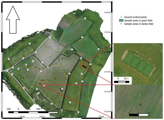
Figure 1.
Test site where barley and grass fields are marked using thick black lines on the orthomosaic based on RGB images from drone. Locations of ground control points and 36 sample plots in barley and 32 sample plots in grass field (zoom) is also marked.
The malt barley Trekker parcels were seeded between 29 May and 6 June 2016. The combined drilling settings for seeding density was 200 kg/ha and for nitrogen input 67.5 kg/ha. Due to relatively cold weather conditions and a short growing season, the barley yield was small (1900 kg/ha) and had a variance of 23.3% [18]. The barley harvesting was made between 23 September and 11 October 2016. The relatively large span in dates was due to the difficult weather conditions. In this study, we used the barley parcel of 20 ha in size. The barley reference measurements were carried out on 8 July 2016 on 36 sample areas that were 50 cm × 50 cm. The field was evenly treated, although a 12-m wide stripe splitting the field was left untreated to provide a bare soil reference. The measurements included the average plant height, fresh yield (FY), dry matter yield (DMY) and amount of nitrogen (Table 1). The coordinates of the sample areas were measured using differentially corrected Trimble GeoXH GPS with an accuracy of 10 cm in the X- and Y-coordinates. The average plant height of each sample spot was measured using a measurement stick. The sample plots were selected so that the vegetation was as homogeneous as possible inside and around the sample areas. Thirteen of the sample plots were located on the spraying tracks that did not include barley (0-squares), however, some weeds were growing in these sample areas, which was important to note during the analysis.

Table 1.
Agricultural sample reference measurements of barley and grass fields: Min: minimum; Max: maximum; Mean: average and standard deviation of the attribute; N of plots: number of sample plots.
The grass silage field was a five-year-old mixture of timothy and meadow fescue. Sample areas were based on eight treatment trial plots, with four replicates conducted by Yara Kotkaniemi Research Station, Yara Suomi Oy, Vihti, Finland (Yara) (https://www.yara.fi/). The nitrogen output for the first cut in every treatment was 120 kg/ha, and the yield level varied between 4497 and 4985 kg/ha of dry matter. The phosphorus (P) level of the grass field site was very low (2.9 mg/L), and different treatments with variable P levels partly explains the yield differences. The reference measurements of a grass parcel were carried out by Yara in the first cut on 13 June 2016 in 32 sample areas (1.5 m × 10 m). Sample areas were harvested with a Haldrup 1500 forage plot harvester. After harvesting, dried samples were analysed in the laboratory. The treatments were combined in the laboratory analysis; thus, the reference FY, DMY and nitrogen measurements were available for eight samples (Table 1).
Altogether 32 permanent ground control points (GCPs) were built and measured in the area. They were marked by wooden poles and targeted with circular targets 30 cm in diameter. Their coordinates in the ETRS-TM35FIN coordinate system were measured using the Trimble R10 (L1 + L2) RTK-GPS. The estimated accuracy of the GCPs was 2 cm in horizontal coordinates and 3 cm in height [56]. Furthermore, three reflectance panels with a nominal reflectance of 0.03, 0.09 and 0.50 [57] were installed in the area to support the radiometric processing.
2.2. Remote Sensing Data
Remote sensing data captures were carried out using a drone and a manned aircraft (Table 2).
Table 2.
Flight parameters of each dataset: date, time, weather, sun azimuth, solar elevation, FH: flight height and FL: number of flight lines. AC RGB: aircraft with RGB camera; AC FPI: aircraft with FPI (Fabry–Pérot interferometer) camera. (In the UAV datasets FPI and RGB cameras were used simultaneously).
A hexacopter drone with a Tarot 960 foldable frame belonging to the FGI was equipped with a hyperspectral camera based on a tuneable FPI and a high-quality Samsung NX500 RGB camera. In this study, the FGI2012b FPI camera [6,7,58] was used; it was configured with 36 spectral bands in the 500 nm to 900 nm spectral range (Table 3). The drone had a NV08C-CSM L1 GNSS receiver (NVS Navigation Technologies Ltd., Montlingen, Switzerland) and a Raspberry Pi single-board computer (Raspberry Pi Foundation, Cambridge, UK). The RGB camera was triggered to take images at two-second intervals, and the GNSS receiver was used to record the exact time of each triggering pulse. The FPI camera had its own GNSS receiver, which collected the exact time of each image. We calculated post-processed kinematic (PPK) GNSS positions for the RGB and FPI cameras’ images, using the NV08C-CSM and the National Land Survey of Finland (NLS) RINEX service [59], using RTKlib software (RTKlib, version 2.4.2, Open-source, Raleigh, NC, USA). UAV data in grass fields was collected using flying heights of 50 m and 140 m and flying speeds of 3.5 m/s and 5 m/s, which provided ground sampling distances (GSDs) of 0.01 m and 0.05 m for RGB images and 0.05 m and 0.14 m for FPI images, respectively. In the barley field, only the flying height of 140 m was used, but four different flights during 3.5 h were necessary to cover the entire test field.
Table 3.
Spectral settings of the hyperspectral camera. L0: central wavelength; FWHM: full width at half maximum.
In the barley field, remote sensing datasets were also captured using a manned small aircraft (Cessna, Wichita, KS, USA) operated by Lentokuva Vallas. The cameras were a RGB camera (Nikon D3X, Tokyo, Japan) and the FPI camera. The RGB data from the aircraft was collected using flying heights of 450 m and 900 m and flying speed of 55 m/s, providing GSDs of 0.05 m and 0.10 m, respectively, for 450 m and 900 m altitudes. The aircraft-based FPI images were captured using a flying height of 700 m and a flying speed of 65 m/s, which provided a GSD of 0.6 m (Table 2). GNSS trajectory data was not available for the aircraft data.
The flight parameters provided image blocks with 73–93% forward and 65–82% side overlaps, which are suitable for accurate photogrammetric processing. In the following, we will refer to the UAV-based sensors as UAV FPI and UAV RGB and the manned aircraft (AC)-based sensors as AC FPI and AC RGB.
2.3. Data Procesing
2.3.1. Geometric Processing
Geometric processing included the determination of the orientations of the images using bundle block adjustment (BBA) and the generation of photogrammetric 3D point cloud. We used Agisoft Photoscan commercial software (version 1.2.5) (AgiSoft LLC, St. Petersburg, Russia). We processed the RGB data separately to obtain a good quality dense point cloud. To obtain good orientations for the FPI images, we performed integrated geometric processing with the RGB images and three bands of the FPI images. The orientations for the rest of the bands of FPI images were calculated using the method developed by Honkavaara et al. [60].
The BBA using Photoscan was supported with five GCPs, and the rest of them [27] were used as checkpoints. The GNSS coordinates of all UAV images, computed using the PPK process, were also applied in the BBA. For the aircraft images, GNSS data was not available. The settings of BBA were selected so that full resolution images were used (quality setting: ‘High’). The settings for the number of key points per image were 40,000 and the number of tie points per image was set at 4000. Furthermore, an automated camera calibration was performed simultaneously with image orientation (self-calibration). The estimated parameters were focal length, principal point, and radial and tangential lens distortion. After initial processing, 10% of the points with the largest uncertainty and reprojection errors were removed automatically, and more clear outliers were removed manually. The outputs of the geometric process were the camera parameters (Interior Orientation Parameters—IOP), the image exterior orientations in the object coordinate system (Exterior Orientation Parameters—EOP) and the 3D coordinates of the tie points (sparse point cloud). The sparse point cloud and the estimated IOP and EOP of three FPI bands (band 3: L0 = 520.4 nm; band 11: L0 = 595.9; band 14: L0 = 625.1 nm) were used as inputs in the 3D band registration process [58]. The processing achieved band registration accuracy better than 1 pixel over the area.
The canopy height model (CHM) was generated using the DSM and digital terrain model (DTM) created by Photoscan using a similar procedure described by Viljanen et al. [25] (Figure 2 and Figure 3). First, the dense point cloud was created using the quality parameter setting ‘Ultrahigh’ and depth filtering setting ‘Mild’; thus, the highest image resolution was used in the dense point cloud generation process. Afterwards, all the points in the dense point cloud were utilized to interpolate the DSM. The DTM was generated from the dense point cloud using Photoscan’s automatic classification procedure for ground points. At first, the dense point cloud was divided into cells of a certain size and the lowest point of each cell was detected. The first approximation of the terrain model was calculated using these points. After that, all points of the dense point cloud were checked, and a new point was added to the ground class if the point was within a certain distance from the terrain model and if the angle between the approximation of the DTM and the line to connect the new point on it was less than a certain angle. Finally, the DTM was interpolated using the points that were classified as ground points.
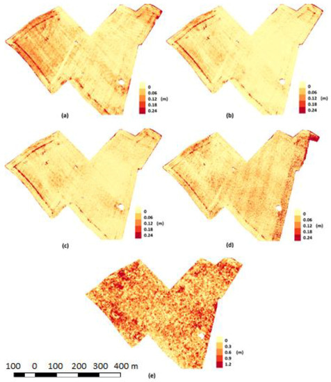
Figure 2.
CHMs (Canopy height model) with barley crop estimates from different datasets: (a) Barley UAV 140 m (RGB) (b) Barley AC 450 m (RGB) (c) Barley AC 900 m (RGB) (d) Barley UAV 140 m (FPI) (e) Barley AC 700 m (FPI).
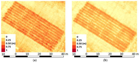
Figure 3.
CHMs (Canopy height model) with grass estimates from different datasets: (a) Grass UAV 50 m (RGB) (b) Grass UAV 140 m (RGB).
The best parameters for the automatic classification procedure of ground points were selected by visually comparing classification results to the orthomosaics. Hence, the cell size of 5 m for the lowest point selection was chosen for all the datasets. For the RGB and FPI datasets, the maximum angle of 0° and 3°, respectively, and the maximum distance of 0.03 m and 0.05 m, respectively, were selected. The parameters are environment- and sensor-resolution-specific, and they differ slightly from the parameters that we used in our previous study on a grass trial site [25] and from the parameters used by Cunliffe et al. [61] in the grass-dominated-shrub ecosystems and by Méndez-Barroso et al. [62] in the forest environment.
The geometric processing indicated good results (Table 4 and Table 5; Figure 2 and Figure 3). The reprojection errors were within 0.46–1.59 pixels. We used 27 checkpoints to evaluate the accuracy of the processing of the barley datasets and 4 checkpoints for the grass datasets. The RMSEs in X and Y coordinates were 1.3–11.3 cm and 5.5–50.9 cm in height (Table 5). A lower flying height resulted in a smaller GSD and also a higher point density. Additionally, increasing the flying height increased the RMSEs in a consistent way. For example, in the case of the grass field, the RMSE in Z coordinate was 6.9 cm and 13.8 cm for the flying heights of 50 m and 140 m, respectively. For the aircraft RGB datasets, the RMSEs in Z-coordinate were 9 cm and 14 cm for the flying heights of 450 m and 900 m, respectively (Table 5).
Table 4.
Dataset parameters: GSD: Ground Sampling Distance, FH: Flight Height, Overlaps in f: flight direction and cf: cross-flight directions; N Images: Number of Images, Re-projection error and Point density.
Table 5.
RMSE: Root Mean Square Errors of X, Y, Z and 3D coordinates were calculated using 27 check points in Barley datasets and 4 in Grass datasets. CHM (Canopy height model) statistics (Mean: average canopy height, Std: Standard deviation of canopy heights; PCC: Pearson Correlation Coefficient of linear regression of reference and CHM-heights, RMSE and Bias: average error) were calculated comparing 90th percentile of CHM in sample plots and ground reference data.
The accuracy of the barley CHMs were evaluated using the plant height measurements of the sample plots as reference and calculating linear regressions between them (Table 5). The 90th percentile of the CHM was used as the height estimate (formula in Section 2.4.2). The best RMSEs were 7.3 cm for the dataset captured using a 140 m flying height (‘Barley UAV 140 m (RGB)’) (Figure 2a). The aircraft-based CHMs for the RGB imagery (’Barley AC 450 m (RGB)’, ‘Barley AC 900 m (RGB)’) also appeared to be non-deformed, but showed lower canopy heights (RMSE: 9.7–10.3 cm) than the UAV-based RGB imagery CHMs (Figure 2a,b,c). In the UAV FPI, CHM striping that followed the flight lines appeared. This indicated that the block was deformed (Figure 2d), and the RMSE of CHM (12.7 cm) was slightly worse than the RGB imagery CHMs. The aircraft FPI-based CHM was clearly deformed and noisier (Figure 2e); it also had the worst RMSE (50.9 cm). Deformation of the FPI-based CHMs was caused by the poorer spatial and radiometric resolution of the images. Except for the poor-quality dataset of CHM “Barley AC 700 m (FPI)”, the bias was negative for all datasets, which indicated that CHM was underestimating the real height of the crop, which is generally an expected result [25] (Table 5).
2.3.2. Radiometric Processing
Radiometric processing of the hyperspectral datasets was carried out using FGI’s RadBA software [7,63]. The objective of the radiometric correction was to provide accurate reflectance orthomosaics. The radiometric modelling approach developed at the FGI included sensor corrections, atmospheric correction, correction for radiometric nonuniformities due to the illumination changes, and the normalization of the object reflectance anisotropy due to illumination and viewing direction related nonuniformities using bidirectional reflectance distribution function (BRDF) correction.
First the sensor response was corrected for the FPI images using the dark signal correction and the photon response nonuniformity correction (PRNU) [6,7]. The dark signal correction was calculated using a black image collected right before the data capture with a covered lens, and the PRNU correction was determined in the laboratory.
The empirical line method [64] was used to calculate the transformation from grey values in images (DN) to reflectance (Refl) for each channel solving following formula:
where and are the parameters of the transformation. Two reference reflectance panels (nominal reflectance 0.03 and 0.10), which were measured with ASD during field work, in the test area were used to determine the parameters.
Because of variable weather conditions during the time of the measurement and other radiometric phenomena, additional radiometric corrections were necessary to obtain uniform orthomosaics. The basic principle of the method is to use the DNs of the radiometric tie points in the overlapping images as observations and to determine the model parameters describing the differences in DNs in different images (the radiometric model) indirectly via the least squares principle. The model for reflectance was
where is the bi-directional reflectance factor (BRF) of the object point, k, in image j; and are the illumination and reflected light (observation) zenith angles, and are the azimuth angles, respectively, and is the relative azimuth angle and is the relative correction parameter with respect to the reference image. The parameters used can be selected according to the demands of the dataset in consideration.
In the case of multiple flights in the UAV based barley dataset, the initial value was based on the irradiance measurements by the ASD and information about integration (exposure) time used in image acquisition:
where ASDj and ASDref are the irradiance measurements and ITj and ITref integration time of sensor during the acquisition of image j and reference image ref. This value was further enhanced in the radiometric block adjustment.
A priori values and standard deviations used in this study (Table 6) were selected based on suggestions by Honkavaara et al. [7,63]. During the drone-based grass data collection, weather was mainly sunny (see Table 2); therefore, we used the BRDF correction to compensate for the reflectance anisotropy effects. For the barley datasets captured by the drone and aircraft, the anisotropy effects did not appear due to the cloudy weather during data collection. In all datasets, it was possible to leave some deviant images unused from the orthomosaics because of the good overlaps between the images. These included some partially shaded images due to clouds in the case of the grass dataset and some images collected under sunshine in the case of the barley dataset.
Table 6.
A priori values for relative image-wise correction parameter (arel:), standard deviations for arel (σa_rel) and image observations (σDN), information about use of BRDF model in the calculations and original and final number of cubes after elimination.
The radiometric block adjustment improved the uniformity of the image orthomosaics, both statistically (Figure 4) and visually (Figure 5). For the uncorrected data, the coefficient of variation (CV) [63] calculated utilizing the overlapping images in the radiometric tie points was higher in the grass data than in the barley data because of the anisotropy effects. This effect is especially visible in the data with the 50 m flying height (Figure 5a). After the radiometric correction, the band-wised CVs were similar for all the drone datasets—approximately 0.05–0.06 (Figure 4). For the aircraft-based datasets, the radiometric block adjustment improved the CVs from the level of 0.13–0.16 to the level of 0.10–0.13, but the uniformity was still not as good as with the drone datasets.
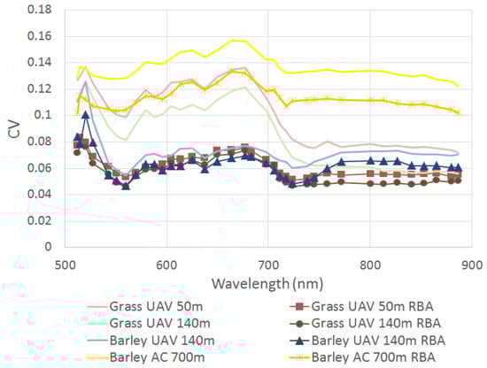
Figure 4.
The coefficient of variation (CV) values of radiometric tie points before (solid lines) and after radiometric block adjustment (RBA, lines with markers) for every 36 spectral band.
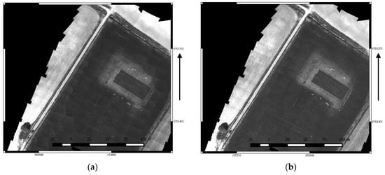
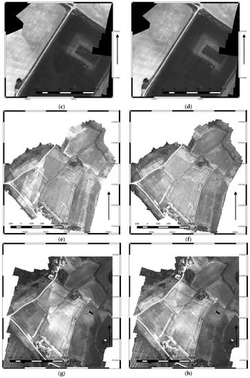
Figure 5.
The reflectance orthomosaics before (a,c,e,g) and after (b,d,f,h) radiometric block adjustment for grass field with 50 m flying height (a,b), 140 m flying height (c,d) and barley field from UAV (e,f) and aircraft (g,h) for band 14 (625.1 nm).
2.3.3. Orthomosaic Generation
The reflectance orthomosaics of the FPI images were calculated using FGI’s RadBA software with different GSDs. The GSD was 0.10 m for the ‘Grass UAV 50 m’, 0.15 m for the ‘Grass UAV 140 m’, 0.20 m for the ‘Barley UAV 140 m’ and 0.60 m for the ‘Barley AC 700 m’. (See the dataset descriptions in Table 4). In the orthomosaics, the most nadir parts of the images were used. The orthomosaics were calculated using both with and without radiometric correction. In the former case, the radiometric correction model described in Section 2.3.2 was used, and in the latter case the DNs were transformed to reflectance using the empirical line method using the reflectance panels without anisotropy or relative radiometric corrections. In the following, the corrected orthomosaics will be indicated with ‘RBA’ (Radiometric Block Adjustment).
The RGB orthomosaics were calculated in Photoscan using the orthomosaic blending mode with a GSD of 0.01 m for the ‘Grass UAV 50 m’ dataset; a GSD of 0.05 m for the ‘Grass UAV 140 m’, ‘Barley UAV 140 m’ and ‘Barley AC 450 m’ datasets; and a GSD of 0.10 m for ‘Barley AC 900 m’. We did not perform the reflectance calibration for the orthomosaics. Instead, the calibration in this case relied on the in situ datasets of agricultural samples.
2.4. Estimation Process
A workflow to estimate agricultural crop parameters using spectral and 3D features were developed in this work (Figure 6). The workflow has four major steps: (1) the field reference measurements; (2) extraction of spectral and 3D features from the hyperspectral and RGB images and the CHM; (3) estimation of the crop parameters with machine learning techniques; and (4) crop parameter map creation and validation of the results. We used Weka software (Weka 3.8.1, University of Waikato) in the estimation, validation and feature selection. These steps are described in detail in the following sections.
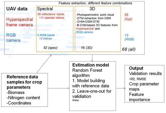
Figure 6.
Workflow to estimate crop parameters using UAV-based spectral (together 52) and 3D (together 16) features. Red colour is indicating features from hyperspectral sensor (together 55) and blue colour RGB sensor (together 13).
We created multiple feature combinations to test performance of different potential sensor setups (FPI, RGB, FPI + RGB), different types of features (spectral, 3D, spectral+3D), the effect of the radiometric processing level, and different spatial resolutions based on flying height (Table 7). We used two different flying heights (50 and 140 m) in the grass field and in the barley field. We used three flying heights with the RGB camera (140, 450 and 900 m) and two with the FPI camera (140 and 700 m), which enabled us to compare the effect of spatial resolution on the estimation results (+barley MAV).
Table 7.
Acronyms for different feature combinations. FPI: FPI (Fabry–Pérot interferometer) camera; spec: spectral features; RBA: radiometric block adjustment; all: all features (spectral and 3D); RGB: RGB camera; 3D: 3D features.
2.4.1. Estimators
We selected the RF and Simple Linear Regression (SLR) as estimators. The validation of the estimation performance was done using leave-one-out cross-validation (LOOCV). In this method, the training and estimation was repeated as many times as there were samples. In each round, the estimator was trained using all samples excluding one; the unused, independent sample was used to calculate the estimation error.
The RF algorithm developed by Breiman [44] is a nonparametric regression approach. Compared with other regression approaches, several advantages have made the RF an attractive tool for regression: it does not overfit when the number of regression trees increases [44], and it does not require variable selection, which could be a difficult task if the number of predictor variables is large. Default parameters of Weka implementations were used, (the number of variables at each split = 100) except the number of decision trees to be generated was set to 500 instead of 100 (number of iterations in Weka), since computation time was not an issue and a large number of trees has often been suggested (for example, Belgiu and Drăguţ, [45]). SLR is traditional and well-known linear regression model with only a single explanatory variable.
2.4.2. Features
We extracted a large number of features from the remote sensing datasets. We used the 36 spectral bands from hyperspectral datasets to create 36 reflectance features (b1-36). The spectral features were extracted to ground samples in an object area of 0.5 m by 0.5 m in the barley field and 1 m by 10 m in the grass field, using QGIS routines (version 2.12.0, Open-source, Raleigh, NC, USA). Furthermore, various vegetation indices (VIs) (Table 8) were selected for biomass and nitrogen estimation. For the RGB camera, DN values (R, B and G) and two indices were used.
Table 8.
Vegetation indices (VI) used in this study.
Furthermore, we extracted 8 different 3D features from the photogrammetric CHMs (2.3.1), including mean, percentiles, standard deviation, minimum and maximum values (Table 9). A Matlab script (version 2016b, MathWorks, Natick, MA, USA) was used to extract features to ground samples.
Table 9.
Definitions and formulas of CHM metrics in this study. hi is the height of the ith height value, N is the total number of height values in the plot, Z is the value from the standard normal distribution for the desired percentile (0 for the 50th, 0.524 for the 70th, 0.842 for the 80th and 1.282, for the 90 percentile) and σ is the standard deviation of the variable.
3. Results
Performance of the estimation process was evaluated using barley and grass field datasets. The results of estimations with the RF are presented in the following sections. In addition, we performed estimations using the SLR to validate the consistency of the RF results. These results are presented in Appendix A.
3.1. Barley Parameter Estimation
3.1.1. Biomass
For the UAV barley datasets, the best biomass estimation results with the highest correlation and lowest RMSE were obtained when using the combination of features from the FPI and RGB cameras and the radiometric correction (‘all RBA’) (Figure 7, Table 10). At best, the correlations and RMSE% were 0.97% and 30.4% for the FY, respectively, and 0.95% and 33.3% for the DMY, respectively. With one exception, the estimation of fresh biomass was more accurate than the estimation of dry biomass. A comparison of RMSE% values in the cases of the datasets with and without a radiometric block adjustment showed that the radiometric adjustment improved the results. For example, when using only the FPI spectral features, the calibration improved results up to 25% (cases: ‘FPI spec’ vs. ‘FPI spec RBA’). The best results were obtained with the spectral features, since adding the 3D features did not significantly improve the estimation results. In the cases with the RGB camera, the RGB spectral features yielded better estimation accuracy than only using 3D features, and combining both gave slightly better estimation accuracy. For example, for the FY, the PCC and RMSE% were 0.95% and 34.5%, respectively, for the combined RGB features (‘RGB all’).
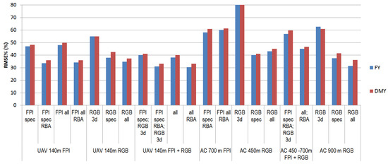
Figure 7.
RMSE% for fresh (FY) and dry (DMY) biomass using varied feature sets in the barley test field. fpi/FPI: FPI camera; spec: spectral features; RBA: radiometric block adjustment; all: all features (spectral and 3D); RGB: RGB camera; 3d: 3D features; UAV: unmanned aerial vehicle; AC: Cessna manned aircraft.
Table 10.
Pearson Correlation Coefficients (PCC), Root mean squared error (RMSE) and RMSE% for fresh (FY) and dry (DMY) biomass using varied feature sets in barley test field. fpi/FPI: FPI camera; spec: spectral features; RBA: radiometric block adjustment; all: all features (spectral and 3D); RGB: RGB camera; 3d: 3D features; UAV: unmanned aerial vehicle; AC: Cessna manned aircraft.
In the cases with the aircraft datasets, the best results were obtained when using the RGB spectral features or a combination of the RGB spectral and 3D features (cases: ‘RGB all’ and ‘RGB spec’). The flying height of 900 m gave slightly better results. At best, the PCC and RMSE% were 0.96% and 31.5%, respectively, in the FY estimation. The estimation results were poorer with the FPI camera than with the RGB camera. This was possibly due to the varying illumination conditions during the FPI-camera flight, which did not provide sufficiently good data quality.
In all cases, the estimations with only the 3D features yielded the worst results. The estimation of FY was more accurate than the estimation of DMY. The RF performed well with various features and combinations and provided in most cases better results than the SLR, but when a limited number of features from one sensor (‘RGB 3D’ and ‘RGB spe’) was used, the SLR yielded better estimation results than the RF (Appendix A; Table A1).
RF provided importance order to the different features used in the experiments. In most cases the indices (such as Cl-red-edge) were more significant spectral features than single reflectance bands. From the 3D features percentiles, p90 was the most important in many cases (Appendix B; Table A4 and Table A5).
3.1.2. Nitrogen
In the case of the UAV datasets, the best estimation accuracy for the barley nitrogen amount and N% were obtained when features from both sensors were applied (‘all RBA’) and with the FPI-based radiometrically corrected spectral features (‘fpi spec RBA’) (Figure 8, Table 11). The radiometric calibration of the FPI data clearly improved the estimation accuracy. The best PCC and RMSE% were 0.97% and 21.6% for the nitrogen amount, respectively, and 0.92% and 34.4% for the N%, respectively. In the case of the UAV RGB sensor, the best accuracy was achieved with the combined data (‘RGB all’). The best PCC and RMSE% were slightly worse than with the FPI data—0.94% and 25.2% for the nitrogen amount, respectively, and 0.92% and 34.5% for the N%, respectively.
Figure 8.
RMSE% for nitrogen (N) and Nitrogen-% in barley test field. fpi/FPI: FPI camera; spec: spectral features; RBA: radiometric block adjustment; all: all features (spectral and 3D); RGB: RGB camera; 3d: 3D features; UAV: unmanned aerial vehicle; AC: Cessna manned aircraft.
Table 11.
Pearson Correlation Coefficients (PCC), Root mean squared error (RMSE) and RMSE% for nitrogen (N) and Nitrogen-% in barley test field. fpi/FPI: FPI camera; spec: spectral features; RBA: radiometric block adjustment; all: all features (spectral and 3D); RGB: RGB camera; 3d: 3D features; UAV: unmanned aerial vehicle; AC: Cessna manned aircraft.
The aircraft based FPI datasets presented the worst estimation accuracy, whereas the estimation results with the RGB features were at the same level as the results of the UAV estimation. For example, the PCC and RMSE% were 0.95% and 25.2%, respectively, for the nitrogen amount and 0.94% and 28.7% for the N% with the RGB spectral features (‘RGB spec’) with the 450 m flight height.
The estimation of the nitrogen amount was more accurate than the estimation of the N%. Regarding the importance of the features, the individual reflectance bands at the red-edge (670–710 nm) were the most important especially for the estimation of N%. In many cases the indices were also considered as the most important. The percentiles (3D features) were important in many cases (Appendix B, Table A6 and Table A7).
3.2. Grass Parameter Estimation
The variation of the biomass and nitrogen amount was low and we had a limited amount of ground samples available in the grass test field. We evaluated the performance using the average of the samples as the estimate. The RF provided better results than using the average value for the biomass estimation, whereas for the nitrogen amount the average was as good as the RF. Therefore, we only studied the biomass estimation. The datasets were captured from the flying heights of 50 m and 140 m using the UAV.
The general view of the results is that the estimation errors were low because of the small variation in the datasets (Table 1). The best PCC and RMSE% were 0.640% and 4.29% for the FY, respectively, and 0.79% and 1.91% for the DMY, respectively (Figure 9, Table 12). These results were obtained with the RGB camera spectral features (‘RGB spec’) captured from the flying height of 140 m. With the FPI camera, the best results were nearly as good, and they were obtained with the radiometrically corrected dataset (‘FPI spec RBA’) from the flying height of 50 m. In this case, the PCC and the RMSE% were 0.538% and 4.63% for the FY, respectively and 0.72% and 2.09% for the DMY, respectively. The radiometric correction with the radiometric block adjustment slightly improved the estimation accuracy in the case of the 50 m dataset, but it did not impact the results for the dataset from the 140 m flying height. It was expected that the radiometric correction would improve the estimation results with the 50 m flying height dataset because it clearly improved the uniformity of the orthomosaics from the 50 m flying height, while for the orthomosaics from the 140 m flying height the correction had a minor impact (Figure 5). The 3D features alone provided the poorest estimation results for both flying heights (‘RGB 3D’), and their use together with the spectral features did not improve the estimation accuracy. The impact of the flying height was minor. The FPI camera dataset with the 50 m flying height provided better results than the dataset with the 140 m flight height. And for the RGB camera, the 140 m dataset provided slightly better results. The estimation accuracies were better for the DMY than for the FY.
Figure 9.
RMSE% for fresh (FY) and dry (DMY) biomass using data collected from 50 m and 140 m flying height in grass test field. fpi/FPI: FPI camera; spec: spectral features; RBA: radiometric block adjustment; all: all features (spectral and 3D); RGB: RGB camera; 3d: 3D features; UAV: unmanned aerial vehicle; AC: Cessna manned aircraft.
Table 12.
Pearson Correlation Coefficients (PCC), Root mean squared error (RMSE) and RMSE%, for fresh (FY) and dry (DMY) biomass using data collected from 50 m and 140 m flying height in grass test field. fpi/FPI: FPI camera; spec: spectral features; RBA: radiometric block adjustment; all: all features (spectral and 3D); RGB: RGB camera; 3d: 3D features; UAV: unmanned aerial vehicle; AC: Cessna manned aircraft.
Similar to barley analysis, the indices, from spectral features, and percentiles, from 3D features, were the most representative features for most of the cases of the grass estimation analysis (Appendix B; Table A8 and Table A9).
4. Discussion
We developed and assessed a machine learning technique integrating 3D and spectral features for the estimation of fresh and dry matter yield (FY, DMY), nitrogen amount and nitrogen percentage (N%) of malt barley crop and grass silage fields. Our approach was to extract a variety of remote sensing features from the datasets that were collected using RGB and imaging hyperspectral cameras. The features included 3D features from the canopy height model (CHM) and spectral features as a spectral, and various vegetation indices (VI) from the orthomosaics. Furthermore, we investigated the impact of the radiometric correction and flying height on the estimation results. Our approach was to use the Random Forest estimator (RF), but the results of the Simple Linear Regression (SLR) estimator was also calculated to validate the performance of the RF.
The best estimation results for the barley biomass and nitrogen content estimations were obtained by combining features from the FPI and RGB cameras. In most cases, the spectral features from the FPI camera provided the most or nearly the most accurate results. Adding the FPI camera 3D features did not improve the results, which was an expected result since FPI based CHM did not have high quality (Table 5, Figure 2d) due to relatively large GSD of 0.14 m. The data from the RGB camera provided good estimation results—typically almost as good as the FPI camera and in some cases the best results. We could also observe that the combination of RGB spectral and 3D features improved the estimation accuracy, especially in the case of biomass estimation. The RF performed well with various features and combinations and provided in most cases better results than the SLR, but some exceptions also appeared (Appendix A; Table A1, Table A2 and Table A3). Especially when only a limited number of features from one sensor (‘RGB 3D’ and ‘RGB spe’) was used, the SLR yielded competitive or even better estimation results than the RF, but when the amount and variation of features was high, the RF provided regularly better estimation results than the SLR. This is a logical performance, because with a small number of features there are not great difference in the SLR and RF models, but with large number of features, the SLR still uses only single feature in the estimation but RF can take advantage of various features during model building. A similar observation was also made by Li et al. [32], where the dry biomass of maize was estimated; they obtained an R2 of 0.52 and an RMSE% of 18.8% with SLR and an R2 of 0.78 and an RMSE% of 16.7% with the RF. The RF thus provided more accurate estimation results. They also concluded that photogrammetric 3D features strongly contributed to the estimation models, in addition to the spectral features from the RGB camera. They suggested that hyperspectral data could improve the estimation results, and our study showed that this was a valid assumption in many situations. Yue et al. [51] compared eight different regression techniques for the winter wheat biomass estimation, using near-surface spectroscopy and achieved R2 values of 0.79–0.89. They concluded that machine learning techniques such as RF were less sensitive to noise than conventional regression techniques.
In the biomass estimations of barley, the PCC and RMSE% were at best 0.95% and 33.2%, respectively, for the DMY, and 0.97% and 31.0%, respectively, for the FY. The corresponding statistics for the grass dataset with the 140 m flying height were 0.79% and 1.9% for the DMY, and 0.64% and 4.3% for the FY, and for the dataset with the flying height of 50 m, the results were on the same level. Concerning the impacts of different features used in the estimations of barley DMY, the inclusion of the 3D features from the RGB camera in addition to the spectral features from the FPI camera improved the RMSEs by 14.7% for uncalibrated FPI, and 7.95% for calibrated FPI. The results were the similar for the barley FY. The possible explanation for this is that the estimation accuracies reached almost the best possible quality with the calibrated spectral features and so the 3D features could not provide further improvement whereas for the uncalibrated spectral features they improved still significantly accuracy. Inclusion of the 3D features based on the FPI camera did not improve the accuracy with either uncalibrated or calibrated data. The reason for this was the insufficient quality of the height data with the FPI camera, and therefore it could not provide quantitative information of differences of various samples to the estimation process. Considering the RGB sensor, the 3D features improved the RMSE% in the DMY and FY estimation by 12.18% and 8.6%, respectively, for barley. The corresponding improvements were 24.2% for the grass DMY and 8.1% for the FY. In the study by Bendig et al. [23], adding the height features with the spectral indices either did not improve or only slightly improved the estimation accuracy of barley biomass when using multilinear regression models. In the study by Yue et al. [24], the correlation between the winter wheat dry biomass and the partial least squares regression (PLS) model based on spectral features was improved from 0.53 to 0.74 and the RMSE from 1.69 to 1.20 t/ha when 3D features were included. These results are comparable to our results for the barley DMY. In studies with spectrally uncalibrated RGB values and 3D features, R2 values of 0.74 have been reported for the corn grain yield estimation [37] and 0.88 for the maize biomass estimation [32], which indicated lower correlations than our results using the RGB data for the barley FMY estimation (PCC = 0.95, RMSE% = 34.74%).
In the nitrogen estimations for barley, the PCC and RMSE% were at best 0.966 and 21.6%, respectively, for the nitrogen amount and 0.919% and 34.4%, respectively, for the N%. Concerning the impacts of different features used in the estimations, the inclusion of the RGB camera 3D features with the spectral features of the FPI camera improved the RMSEs (0–30%), which indicated that the 3D features provided additional information to the estimation model. Also combining the 3D features to the RGB spectral features improved the estimation accuracy of the nitrogen amount and the N% by 12.5% and 23.6%, respectively, providing similar accuracy as the FPI based spectral features. It is worth noting, that even though the variation of N% on sample references was not high (Table 1), good accuracies were achieved. The variation in the nitrogen amount was mainly related to variation in the biomass amount, which explains the similar estimation accuracies of the two quantities. Liu et al. [50] used several different algorithms to estimate the nitrogen content (N%) of winter wheat based on multispectral data and achieved the best results with an R2 of 0.79 and an RMSE% of 11.56% with the RF. Geipel et al. [37] used SLR models based on a multispectral sensor to estimate the N content and achieved accuracies with an R2 of 0.58–0.89 and an RMSE% of 7.6–11.7%. Schirrmann et al. [42] achieved at the best R2 value of 0.65 between the nitrogen content and the principal components of RGB image. Our results were on the same level with Liu et al. [50], Geipel et al. [37] and Schirrmann et al. [42]; but with terrestrial approaches, even higher accuracies have been achieved [52]. Furthermore, data from tractor-mounted Yara N-sensor has reported good correlations of R2 0.80 with N-uptake in grass sward [54]. However, it is important to notice that the estimation accuracies of different studies are not directly comparable because they are also impacted by the properties of the crop sample data, such as the variation in their values.
When comparing the estimation accuracy with the spectral features only from the FPI and RGB cameras, the FPI camera provided 15.4% and 18.5% better RMSEs than the RGB camera for the barley DMY and FY, respectively, but up to 16.5% and 14.4% worse RMSEs than the RGB camera for the grass DMY and FY, respectively. Better performance of the FPI camera was expected since the hyperspectral images provide more spectral information than the RGB images. The challenges with the grass study were the small number of samples and the small variation in the biomass amount, and therefore the grass results should be considered as indicative. In the estimation of the nitrogen, the FPI camera outperformed the RGB camera by 25.0% for the barley nitrogen amount and by 21.1% for the barley N%. The nitrogen content of plants is relatively small (Table 1), thus it is expected that they only slightly affect the spectra. Consequently, FPI provides higher accuracy than RGB, because it is collecting more information from spectra.
In most cases, the radiometric calibration of the datasets using the radiometric block adjustment improved the estimation results. In the case of barley parameter estimations with all features, the radiometric correction improved the RMSE by 17.0% for the DMY, 20.3% for the FY and 25.0% for the nitrogen amount. In the case of the grass estimation, the impact was smaller—the correction either slightly decreased or improved the RMSE by −6.3–3.6% for the DMY and 0–2.4% for the FY. The improvement was largest in the datasets having many flight lines (Table 2). The effect was the most noticeable in the ‘Barley UAV 140 m’ dataset, which was collected during 4.5 h, when illumination changed significantly, and in the ‘Grass UAV 50 m’ dataset, which was collected during sunny conditions at a low flying height that caused remarkable anisotropy effects (Figure 5). Multiple studies have shown that radiometric correction using the RBA method improved the uniformity of image orthomosaics [7,11,12,63,77]. Our results showed that the corrections also improved the accuracy of the crop parameter estimations.
The barley datasets were collected from the UAV and aircraft using various flying heights, which provided different GSDs. In the case of the RGB camera, the GSDs were 0.05 and 0.10 m, and the estimation results were similar when spectral features were applied. However, the flying height and GSD had a significant impact on the accuracy of the 3D features, which we could already deduce based on the CHM quality (Table 5, Figure 2 and Figure 3). The most reliable CHM was obtained using data with the smallest GSD, ‘Barley UAV 140 m RGB’, where the correlation between in situ reference measurements and the CHM were highest, even though the CHM regularly underestimated in situ measurements (Figure 2a). The quality of the DSM decreased when the GSD increased, and when the GSD was too large (like in the case of ‘Barley AC 700 m FPI’ with a GSD of 0.60 m), the 3D features were useless. It is also important to notice that in all cases, the height accuracy of the blocks was good and according to expectations—on the level of 0.5–2 times the GSD. At the smallest GSDs, the UAV and aircraft provided comparable accuracies. Thus the low-cost sensors used in this study can also be operated from small aircraft. The advantage of the aircraft-based method is that larger areas can be covered more efficiently. However, in smaller areas drones are more affordable.
It is worth noting that in the barley field the growth was not ideal due to poor weather conditions at the beginning of the growing season. In the grass canopy, the number of field reference samples were relatively low (8 samples) and variation in the biomass and nitrogen amounts was low, which generally decreases the correlation and estimation results. However, if we think practical solution for crop parameter estimation, collection of even a small number of samples is time-consuming and increase costs. The result with a few samples with a small variation was slightly better than when using the average value as the estimate; this indicated that with the comprehensive machine learning method the estimation accuracy could be improved from the case of using only average values, as it revealed relatively small spatial variations. Although we obtained promising results using datasets from the 140 m or higher flight heights, the use of lower height data, and thus more precise CHMs, can improve the estimations, as shown in previous studies using flight heights of 50 m or less [4,21,25]. We assume that the spatial and radiometric resolution of the images are the fundamental factors impacting the quality of CHM thus we expect that alternatively a better-quality imaging system could also provide good results from higher altitudes; this would be advantageous if aiming at mapping larger areas.
To our knowledge, this study was the first one that comprehensively integrated and compared UAV-based hyperspectral, RGB and point cloud features in crop parameter estimation. We developed an approach for utilizing a combination of spectral data and 3D features in the estimation process that simultaneously and efficiently utilizes all available information. Furthermore, our results showed that the integration of spectral and 3D features improved the accuracy of the biomass estimation; but in the nitrogen estimation, the spectral features were more important. The results also indicated that the hyperspectral data provided only a slight or no improvement to the estimation accuracy of the biomass compared to the RGB data. This result thus suggests that the low-cost RGB sensors are suitable for the biomass estimation task. However, more studies are recommended to validate this result in different conditions. In the nitrogen estimation, the hyperspectral data appeared to be more advantageous than the RGB data. The aircraft-based data capture also provided results comparable to the UAV-based results.
In the future, further studies using more accurate hyperspectral sensors and higher variability test sites will be of interest. The datasets also give possibilities for new types of analysis, such as utilizing the spectral DSM more rigorously [21,22] and utilizing the multiview spectral datasets in the analysis [78,79,80]. Our future objective will be to develop generalized estimators that can be used without in situ training data, for example, training an estimator with a dataset from one sample area and then using it in other areas. Various machine learning techniques exist that can be used in this process. Our results showed that the SLR was not ideal for this task. The RF behaved well, and further studies will be necessary to evaluate its suitability for the generalized procedures. For example, the deep learning neural network estimators will be very interesting alternatives [81].
5. Conclusions
We developed and assessed a machine learning technique integrating 3D and spectral features for the estimation of fresh and dry matter yield (FY, DMY), nitrogen content and nitrogen percentage (N%) of barley crops and grass silages. Our approach was to extract a large number of remote sensing features from the datasets, including 3D features from the canopy height model (CHM) and hyperspectral features and various vegetation indices (VI) from orthomosaics. Furthermore, we investigated the impact of radiometric correction on the estimation results. We compared the performance of Simple Linear Regression (SLR) and the Random Forest estimator (RF). To our knowledge, this study was one of the first studies to integrate and compare UAV-based hyperspectral, RGB and point cloud features in the estimation process. Generally, the best results were obtained when integrating hyperspectral and 3D features. The integration of RGB and 3D features also provided nearly as good results as the hyperspectral features. The integration of spectral and 3D features especially improved the biomass estimation results. The radiometric calibration improved the estimation accuracy, and we expect that it will be one of the prerequisites in developing generalized analysis tools. Our important future research objective will be to develop generalized estimation tools that do not require in situ training data.
Author Contributions
The experiment was designed by E.H. and J.K. J.K. and K.A. corresponded about the agricultural test field design and E.H. corresponded about the remote sensing test field design. T.H., R.N., and N.V. carried out the imaging flights. N.V. carried out the geometric and R.N. and L.M. radiometric processing steps. R.N. developed the estimation methods and performed the estimations; analysis of the results was made by R.N. and E.H. The article was written by R.N., N.V. and E.H., with the assistance of other authors.
Funding
This work was funded by the ICT Agri ERA-NET 2015 Enabling precision farming project GrassQ-Development of ground based and Remote Sensing, automated “real-time” grass quality measurement to enhance grassland management information platforms (Project id 35779), and the Academy of Finland project “Quantitative remote sensing by 3D hyperspectral UAVs—From theory to practice” (grant No. 305994).
Conflicts of Interest
The authors declare no conflict of interest.
Appendix A
Table A1.
Pearson Correlation Coefficients (PCC), Root mean squared error (RMSE) and RMSE% for fresh (FY) and dry (DMY) biomass using varied feature sets in barley test field using SLR.
Table A1.
Pearson Correlation Coefficients (PCC), Root mean squared error (RMSE) and RMSE% for fresh (FY) and dry (DMY) biomass using varied feature sets in barley test field using SLR.
| FY Barley | DMY Barley | |||||
|---|---|---|---|---|---|---|
| PCC | RMSE | RMSE% | PCC | RMSE | RMSE% | |
| Flying height 140 m UAV | ||||||
| fpi spec | 0.924 | 0.196 | 42.2 | 0.872 | 0.038 | 51.2 |
| fpi spec RBA | 0.919 | 0.203 | 43.7 | 0.918 | 0.030 | 41.4 |
| fpi all | 0.873 | 0.250 | 53.7 | 0.872 | 0.038 | 51.2 |
| fpi all RBA | 0.935 | 0.182 | 39.1 | 0.918 | 0.030 | 41.4 |
| RGB 3d | 0.924 | 0.196 | 42.2 | 0.906 | 0.032 | 44.2 |
| RGB spec | 0.956 | 0.151 | 32.5 | 0.940 | 0.026 | 35.6 |
| RGB all | 0.956 | 0.151 | 32.5 | 0.940 | 0.026 | 35.6 |
| fpi spec; RGB 3d | 0.873 | 0.250 | 53.7 | 0.873 | 0.038 | 51.2 |
| fpi spec RBA; RGB 3d | 0.935 | 0.182 | 39.1 | 0.918 | 0.030 | 41.4 |
| all | 0.956 | 0.151 | 32.5 | 0.940 | 0.026 | 35.6 |
| all RBA | 0.956 | 0.151 | 32.5 | 0.940 | 0.026 | 35.6 |
| Flying height 450–700 m AC | ||||||
| fpi spec RBA | 0.788 | 0.315 | 67.8 | 0.771 | 0.049 | 66.6 |
| fpi all RBA | 0.788 | 0.315 | 67.8 | 0.771 | 0.049 | 66.6 |
| RGB 3d | 0.731 | 0.351 | 75.5 | 0.689 | 0.056 | 76.3 |
| RGB spec | 0.919 | 0.201 | 43.3 | 0.911 | 0.032 | 43.1 |
| RGB all | 0.919 | 0.201 | 43.3 | 0.911 | 0.032 | 43.1 |
| fpi spec RBA; RGB 3d | 0.714 | 0.361 | 77.6 | 0.771 | 0.049 | 66.6 |
| all; RBA | 0.919 | 0.201 | 43.3 | 0.911 | 0.032 | 43.1 |
| Flying height 900 m AC | ||||||
| RGB 3d | 0.738 | 0.349 | 75.0 | 0.693 | 0.056 | 76.3 |
| RGB spec | 0.935 | 0.181 | 39.0 | 0.925 | 0.029 | 39.6 |
| RGB all | 0.935 | 0.181 | 39.0 | 0.925 | 0.029 | 39.6 |
Table A2.
Pearson Correlation Coefficients (PCC), Root mean squared error (RMSE) and RMSE% for nitrogen (N) and Nitrogen-% in barley test field using SLR.
Table A2.
Pearson Correlation Coefficients (PCC), Root mean squared error (RMSE) and RMSE% for nitrogen (N) and Nitrogen-% in barley test field using SLR.
| N Barley | N% Barley | |||||
|---|---|---|---|---|---|---|
| PCC | RMSE | RMSE% | PCC | RMSE | RMSE% | |
| Flying height 140 m UAV | ||||||
| fpi spec | 0.927 | 0.001 | 28.8 | 0.770 | 0.937 | 54.7 |
| fpi spec RBA | 0.917 | 0.001 | 32.4 | 0.795 | 0.893 | 52.2 |
| fpi all | 0.834 | 0.001 | 43.2 | 0.770 | 0.937 | 54.7 |
| fpi all RBA | 0.938 | 0.001 | 28.8 | 0.795 | 0.893 | 52.2 |
| RGB 3d | 0.927 | 0.001 | 28.8 | 0.704 | 1.046 | 61.1 |
| RGB spec | 0.964 | 0.001 | 21.6 | 0.764 | 0.948 | 55.4 |
| RGB all | 0.964 | 0.001 | 21.6 | 0.764 | 0.948 | 55.4 |
| fpi spec; RGB 3d | 0.834 | 0.001 | 43.2 | 0.770 | 0.937 | 54.7 |
| fpi spec RBA; RGB 3d | 0.938 | 0.001 | 28.8 | 0.795 | 0.893 | 52.2 |
| all | 0.964 | 0.001 | 21.6 | 0.722 | 1.022 | 59.7 |
| all RBA | 0.964 | 0.001 | 21.6 | 0.795 | 0.893 | 52.2 |
| Flying height 450–700 m AC | ||||||
| fpi spec RBA | 0.741 | 0.002 | 54.0 | 0.507 | 1.320 | 77.1 |
| fpi all RBA | 0.741 | 0.002 | 54.0 | 0.507 | 1.320 | 77.1 |
| RGB 3d | 0.725 | 0.002 | 54.0 | 0.228 | 1.555 | 90.8 |
| RGB spec | 0.949 | 0.001 | 25.2 | 0.847 | 0.781 | 45.6 |
| RGB all | 0.949 | 0.001 | 25.2 | 0.847 | 0.781 | 45.6 |
| fpi spec RBA; RGB 3d | 0.741 | 0.002 | 54.0 | 0.507 | 1.320 | 77.1 |
| all; RBA | 0.949 | 0.001 | 25.2 | 0.847 | 0.781 | 45.6 |
| Flying height 900 m AC | ||||||
| RGB 3d | 0.715 | 0.002 | 57.6 | 0.193 | 1.514 | 88.5 |
| RGB spec | 0.959 | 0.001 | 21.6 | 0.854 | 0.765 | 44.7 |
| RGB all | 0.959 | 0.001 | 21.6 | 0.854 | 0.765 | 44.7 |
Table A3.
Pearson Correlation Coefficients (PCC), Root mean squared error (RMSE) and RMSE%, for fresh (FY) and dry (DMY) biomass using data collected from 50 and 140 m flying height in grass test field.
Table A3.
Pearson Correlation Coefficients (PCC), Root mean squared error (RMSE) and RMSE%, for fresh (FY) and dry (DMY) biomass using data collected from 50 and 140 m flying height in grass test field.
| FY Barley | DMY Barley | |||||
|---|---|---|---|---|---|---|
| PCC | RMSE | RMSE% | PCC | RMSE | RMSE% | |
| Flying height 50 m | ||||||
| FPI spec | 0.332 | 0.107 | 6.2 | 0.436 | 0.015 | 3.1 |
| FPI spec RBA | 0.712 | 0.077 | 4.5 | 0.847 | 0.008 | 1.6 |
| RGB 3D | 0.332 | 0.105 | 6.1 | 0.378 | 0.015 | 3.1 |
| RGB spe | 0.367 | 0.100 | 5.8 | 0.446 | 0.015 | 3.1 |
| RGB all | 0.203 | 0.114 | 6.6 | 0.446 | 0.015 | 3.1 |
| FPI spec; RGB 3D | 0.332 | 0.107 | 6.2 | 0.436 | 0.015 | 3.1 |
| FPI spec RBA; RGB 3D | 0.712 | 0.077 | 4.5 | 0.847 | 0.008 | 1.6 |
| Flying height 140 m | ||||||
| FPI spec | 0.515 | 0.087 | 5.0 | 0.732 | 0.011 | 2.3 |
| FPI spec RBA | 0.527 | 0.081 | 4.7 | 0.577 | 0.013 | 2.6 |
| RGB 3D | 0.822 | 0.055 | 3.2 | 0.390 | 0.017 | 3.5 |
| RGB spe | 0.711 | 0.069 | 4.0 | 0.742 | 0.012 | 2.5 |
| RGB all | 0.754 | 0.064 | 3.7 | 0.742 | 0.012 | 2.5 |
| FPI spec; RGB 3D | 0.596 | 0.088 | 5.1 | 0.732 | 0.011 | 2.3 |
| FPI spec RBA; RGB 3D | 0.683 | 0.076 | 4.4 | 0.577 | 0.013 | 2.6 |
Appendix B
Table A4.
The most important features for the Random Forest (RF) (in the order of importance) for FY estimation in barley.
Table A4.
The most important features for the Random Forest (RF) (in the order of importance) for FY estimation in barley.
| Flying height 140 m UAV | |||||||
| fpi spec | Cl-RE | Cl-Gr | RDVI | MTVI | b34 | NDVI | b19 |
| fpi spec RBA | b21 | b20 | Cl-Gr | Cl-RE | b17 | b15 | b19 |
| fpi all | Cl-RE | MTVI | Cl-Gr | OSAVI | RDVI | NDVI | b33 |
| fpi all RBA | Cl-RE | Cl-Gr | b20 | GNDVI | b15 | b19 | b17 |
| RGB 3d | RGB_CHMp90 | RGB_CHMp80 | RGB_CHMp50 | RGB_CHMp70 | RGB_CHMmax | RGB_CHMmin | RGB_CHMmean |
| RGB spec | RGB-GRVI | RGB-ExG | RGB-R | RGB-B | RGB-G | NaN | NaN |
| RGB all | RGB-R | RGB-GRVI | RGB-ExG | RGB_CHMp90 | RGB_CHMp80 | RGB-B | RGB_CHMp70 |
| fpi spec; RGB 3d | MTVI | Cl-RE | OSAVI | Cl-Gr | NDVI | RGB_CHMmax | b18 |
| fpi spec RBA; RGB 3d | Cl-Gr | b16 | b20 | b17 | Cl-RE | MTVI | b18 |
| all | Cl-RE | RGB-GRVI | RGB-R | RGB-ExG | OSAVI | MTVI | RGB-B |
| all RBA | RGB-R | b21 | RGB-ExG | b15 | b19 | b17 | OSAVI |
| Flying height 450–700 m AC | |||||||
| fpi spec RBA | MTVI | OSAVI | NDVI | RDVI | Cl-RE | b20 | GNDVI |
| fpi all RBA | MTVI | Cl-RE | OSAVI | NDVI | b20 | b19 | b18 |
| RGB 3d | CHMp90 | CHMp50 | CHMp80 | CHMmin | CHMp70 | CHMmax | CHMmean |
| RGB spec | GRVI | B | R | ExG | G | NaN | NaN |
| RGB all | GRVI | B | R | CHMp50 | ExG | CHMp90 | G |
| fpi spec RBA; RGB 3d | MTVI | b20 | OSAVI | Cl-RE | b19 | NDVI | RDVI |
| all; RBA | MTVI | Cl-RE | OSAVI | GRVI | R | RDVI | NDVI |
| Flying height 900 m AC | |||||||
| RGB 3d | CHMp80 | CHMp90 | CHMp70 | CHMmax | CHMp50 | CHMmin | CHMmean |
| RGB spec | B | GRVI | G | ExG | R | NaN | NaN |
| RGB all | ExG | GRVI | B | G | CHMp90 | CHMp80 | R |
Table A5.
The most important features for the Random Forest (RF) (in the order of importance) for DMY estimation in barley.
Table A5.
The most important features for the Random Forest (RF) (in the order of importance) for DMY estimation in barley.
| Flying height 140 m UAV | |||||||
| fpi spec | Cl-Gr | Cl-RE | RDVI | MTVI | NDVI | OSAVI | GNDVI |
| fpi spec RBA | Cl-RE | MTVI | RDVI | GNDVI | b32 | NDVI | b30 |
| fpi all | Cl-Gr | Cl-RE | OSAVI | MTVI | RDVI | NDVI | b36 |
| fpi all RBA | Cl-RE | MTVI | NDVI | GNDVI | b32 | RDVI | Cl-Gr |
| RGB 3d | RGB_CHMp90 | RGB_CHMp80 | RGB_CHMp70 | RGB_CHMmax | RGB_CHMp50 | RGB_CHMmean | RGB_CHMmin |
| RGB spec | RGB-ExG | RGB-GRVI | RGB-R | RGB-B | RGB-G | NaN | NaN |
| RGB all | RGB_CHMp90 | RGB-ExG | RGB-GRVI | RGB_CHMp80 | RGB-R | RGB_CHMp70 | RGB_CHMmax |
| fpi spec; RGB 3d | MTVI | Cl-Gr | Cl-RE | RGB_CHMp80 | RGB_CHMp90 | RDVI | RGB_CHMmax |
| fpi spec RBA; RGB 3d | MTVI | Cl-RE | RDVI | GNDVI | b32 | Cl-Gr | OSAVI |
| all | Cl-RE | RGB-ExG | RGB-GRVI | RGB-R | OSAVI | RGB_CHMp90 | Cl-Gr |
| all RBA | Cl-RE | OSAVI | RDVI | Cl-Gr | RGB_CHMp80 | RGB-GRVI | GNDVI |
| Flying height 450–700 m AC | |||||||
| fpi spec RBA | MTVI | OSAVI | NDVI | GNDVI | b17 | Cl-RE | b36 |
| fpi all RBA | OSAVI | MTVI | NDVI | Cl-RE | GNDVI | RDVI | b20 |
| RGB 3d | CHMp50 | CHMp90 | CHMp70 | CHMp80 | CHMmin | CHMmax | CHMstd |
| RGB spec | ExG | B | GRVI | R | G | NaN | NaN |
| RGB all | ExG | GRVI | B | R | G | CHMp80 | CHMmin |
| fpi spec RBA; RGB 3d | MTVI | b20 | NDVI | OSAVI | Cl-RE | RDVI | b19 |
| all; RBA | OSAVI | GRVI | ExG | MTVI | Cl-RE | R | RDVI |
| Flying height 900 m AC | |||||||
| RGB 3d | CHMp80 | CHMp90 | CHMp70 | CHMmax | CHMp50 | CHMmin | CHMmean |
| RGB spec | GRVI | ExG | B | R | G | NaN | NaN |
| RGB all | GRVI | CHMp80 | ExG | R | B | CHMp90 | G |
Table A6.
The most important features for the Random Forest (RF) (in the order of importance) for nitrogen estimation in barley.
Table A6.
The most important features for the Random Forest (RF) (in the order of importance) for nitrogen estimation in barley.
| Flying height 140 m UAV | |||||||
| fpi spec | Cl-Gr | Cl-RE | b18 | b20 | RDVI | b19 | b17 |
| fpi spec RBA | b15 | b17 | Cl-RE | b20 | b18 | b21 | NDVI |
| fpi all | Cl-Gr | b18 | Cl-RE | b20 | RDVI | MTVI | b19 |
| fpi all RBA | Cl-RE | b18 | b21 | b16 | b15 | b17 | b20 |
| RGB 3d | CHMp90 | CHMp80 | CHMmax | CHMmin | CHMp50 | CHMp70 | CHMmean |
| RGB spec | RGB-GRVI | RGB-R | RGB-ExG | RGB-G | RGB-B | ||
| RGB all | CHMp90 | CHMp80 | RGB-GRVI | CHMp70 | RGB-R | CHMmax | RGB-ExG |
| fpi spec; RGB 3d | MTVI | b19 | Cl-Gr | b18 | Cl-RE | CHMmax | RDVI |
| fpi spec RBA; RGB 3d | b17 | b18 | b20 | MTVI | Cl-RE | CHMmax | b19 |
| all | MTVI | RGB-GRVI | b19 | CHMp90 | CHMmax | Cl-RE | RGB-R |
| all RBA | Cl-RE | b17 | GNDVI | b19 | NDVI | OSAVI | RGB-R |
| Flying height 450–700 m AC | |||||||
| fpi spec RBA | MTVI | NDVI | b19 | Cl-RE | OSAVI | b15 | b17 |
| fpi all RBA | MTVI | NDVI | b20 | Cl-RE | b19 | b18 | b14 |
| RGB 3d | CHMp50 | CHMp80 | CHMp90 | CHMp70 | CHMmin | CHMmax | CHMmean |
| RGB spec | GRVI | G | R | ExG | B | ||
| RGB all | GRVI | ExG | CHMp90 | R | G | CHMp70 | B |
| fpi spec RBA; RGB 3d | MTVI | b20 | OSAVI | b15 | b19 | b18 | NDVI |
| all; RBA | b17 | b19 | Cl-RE | b20 | Cl-Gr | MTVI | GRVI |
| Flying height 900 m AC | |||||||
| RGB 3d | CHMp80 | CHMp90 | CHMp70 | CHMmax | CHMp50 | CHMmean | CHMmin |
| RGB spec | GRVI | R | G | B | ExG | ||
| RGB all | GRVI | G | R | ExG | B | CHMp90 | CHMp80 |
Table A7.
The most important features for the Random Forest (RF) (in the order of importance) for N% estimation in barley.
Table A7.
The most important features for the Random Forest (RF) (in the order of importance) for N% estimation in barley.
| Flying height 140 m UAV | |||||||
| fpi spec | b19 | MTVI | b18 | b20 | OSAVI | b17 | b21 |
| fpi spec RBA | NDVI | b15 | b21 | OSAVI | b19 | b17 | b18 |
| fpi all | Cl-RE | b20 | OSAVI | b18 | MTVI | b17 | NDVI |
| fpi all RBA | NDVI | b19 | b18 | b21 | PRI | OSAVI | b15 |
| RGB 3d | CHMp50 | CHMp70 | CHMmin | CHMp80 | CHMmean | CHMp90 | CHMmax |
| RGB spec | RGB-GRVI | RGB-ExG | RGB-R | RGB-B | RGB-G | NaN | NaN |
| RGB all | CHMp70 | CHMp80 | CHMp50 | CHMp90 | CHMmin | RGB-GRVI | CHMmean |
| fpi spec; RGB 3d | MTVI | CHMp90 | CHMmean | CHMp80 | b19 | CHMp50 | CHMp70 |
| fpi spec RBA; RGB 3d | b19 | MTVI | b15 | PRI | CHMp80 | CHMmin | NDVI |
| all | CHMmean | MTVI | CHMp50 | RGB-GRVI | CHMp90 | b19 | CHMp70 |
| all RBA | CHMmin | RGB-GRVI | b21 | CHMp90 | b19 | NDVI | CHMmean |
| Flying height 450–700 m AC | |||||||
| fpi spec RBA | b19 | b20 | b18 | b17 | b13 | b21 | b16 |
| fpi all RBA | b19 | b21 | b20 | b17 | b18 | b16 | b13 |
| RGB 3d | CHMp70 | CHMp80 | CHMp50 | CHMp90 | CHMmax | CHMstd | CHMmin |
| RGB spec | GRVI | B | R | G | ExG | NaN | NaN |
| RGB all | GRVI | R | B | G | ExG | CHMp80 | CHMp70 |
| fpi spec RBA; RGB 3d | b20 | b19 | b17 | b18 | b15 | b13 | CHMp50 |
| all; RBA | b19 | b20 | GRVI | R | B | G | ExG |
| Flying height 900 m AC | |||||||
| RGB 3d | CHMp90 | CHMp80 | CHMp70 | CHMmax | CHMp50 | CHMstd | CHMmean |
| RGB spec | B | GRVI | R | G | ExG | NaN | NaN |
| RGB all | B | G | GRVI | R | ExG | CHMp90 | CHMp80 |
Table A8.
The most important features for the Random Forest (RF) (in the order of importance) for FY estimation in grass.
Table A8.
The most important features for the Random Forest (RF) (in the order of importance) for FY estimation in grass.
| Flying height 50 m | |||||||
| FPI spec | Cl-Gr | MTVI | b34 | b24 | b26 | b8 | b28 |
| FPI spec RBA | MCARI | b24 | b14 | MTVI | NDVI | b20 | b6 |
| RGB 3D | CHMp90 | CHMmax | CHMp80 | CHMp70 | CHMmean | CHMstd | CHMp50 |
| RGB spe | exG | r | g | grv | b | NaN | NaN |
| RGB all | exG | CHMp90 | CHMmax | g | CHMp70 | CHMp80 | CHMmean |
| FPI spec; RGB 3D | CHMp90 | b34 | b9 | REIP | b7 | b32 | b28 |
| FPI spec RBA; RGB 3D | b24 | b27 | b14 | CHMp90 | b4 | CHMmax | b25 |
| Flying height 140 m | |||||||
| FPI spec | b36 | b24 | b31 | b29 | b5 | b34 | b7 |
| FPI spec RBA | MTVI | RDVI | b32 | b34 | b30 | b31 | b35 |
| RGB 3D | CHMp90 | CHMp80 | CHMp70 | CHMstd | CHMmin | CHMmax | CHMp50 |
| RGB spe | g | r | exG | b | grv | NaN | NaN |
| RGB all | CHMp90 | b | exG | g | r | CHMp70 | CHMstd |
| FPI spec; RGB 3D | Cl-Gr | b35 | b31 | b30 | b24 | b28 | b34 |
| FPI spec RBA; RGB 3D | RDVI | b30 | MCARI | b36 | b31 | b6 | b26 |
Table A9.
The most important features for the Random Forest (RF) (in the order of importance) for DMY estimation in grass.
Table A9.
The most important features for the Random Forest (RF) (in the order of importance) for DMY estimation in grass.
| Flying height 50 m | |||||||
| FPI spec | Cl-Gr | RDVI | GNDVI | REIP | b26 | b25 | b32 |
| FPI spec RBA | MTCI | PRI | GNDVI | NDVI | b22 | OSAVI | Cl-RE |
| RGB 3D | CHMp70 | CHMp90 | CHMp80 | CHMmax | CHMp50 | CHMmean | CHMstd |
| RGB spe | grv | exG | b | g | r | NaN | NaN |
| RGB all | g | r | exG | grv | b | CHMp90 | CHMp70 |
| FPI spec; RGB 3D | OSAVI | Cl-RE | MTVI | b36 | b27 | RDVI | GNDVI |
| FPI spec RBA; RGB 3D | PRI | OSAVI | Cl-Gr | b24 | MCARI | MTCI | b16 |
| Flying height 140 m | |||||||
| FPI spec | Cl-Gr | GNDVI | REIP | b22 | b30 | b20 | b28 |
| FPI spec RBA | GNDVI | b36 | b24 | MTCI | b33 | OSAVI | b22 |
| RGB 3D | CHMp80 | CHMp90 | CHMp70 | CHMstd | CHMmin | CHMmax | CHMmean |
| RGB spe | grv | exG | g | r | b | NaN | NaN |
| RGB all | exG | b | grv | g | r | CHMstd | CHMp80 |
| FPI spec; RGB 3D | Cl-RE | OSAVI | GNDVI | b25 | b22 | MTVI | b21 |
| FPI spec RBA; RGB 3D | b33 | b32 | b34 | b24 | b16 | GNDVI | b31 |
References
- Yang, G.; Liu, J.; Zhao, C.; Li, Z.; Huang, Y.; Yu, H.; Xu, B.; Yang, X.; Zhu, D.; Zhang, X.; et al. Unmanned aerial vehicle remote sensing for field-based crop phenotyping: Current status and perspectives. Front. Plant Sci. 2017, 8. [Google Scholar] [CrossRef] [PubMed]
- Balafoutis, A.; Beck, B.; Fountas, S.; Vangeyte, J.; Wal, T.; van der Soto, I.; Gómez-Barbero, M.; Barnes, A.; Eory, V. Precision agriculture technologies positively contributing to GHG emissions mitigation, farm productivity and economics. Sustainability 2017, 9, 1339. [Google Scholar] [CrossRef]
- Mulla, D.J. Twenty five years of remote sensing in precision agriculture: Key advances and remaining knowledge gaps. Biosyst. Eng. 2013, 114, 358–371. [Google Scholar] [CrossRef]
- Sankaran, S.; Khot, L.R.; Espinoza, C.Z.; Jarolmasjed, S.; Sathuvalli, V.R.; Vandemark, G.J.; Miklas, P.N.; Carter, A.H.; Pumphrey, M.O.; Knowles, N.R.; et al. Low-altitude, high-resolution aerial imaging systems for row and field crop phenotyping: A review. Eur. J. Agron. 2015, 70, 112–123. [Google Scholar] [CrossRef]
- Saari, H.; Pellikka, I.; Pesonen, L.; Tuominen, S.; Heikkilä, J.; Holmlund, C.; Mäkynen, J.; Ojala, K.; Antila, T. Unmanned aerial vehicle (UAV) operated spectral camera system for forest and agriculture applications. In Remote Sensing for Agriculture, Ecosystems, and Hydrology XIII; International Society for Optics and Photonics: Bellingham, WA, USA, 2011; Volume 8174, p. 81740H. [Google Scholar]
- Mäkynen, J.; Holmlund, C.; Saari, H.; Ojala, K.; Antila, T. Unmanned aerial vehicle (UAV) operated megapixel spectral camera. In Electro-Optical Remote Sensing, Photonic Technologies, and Applications V; International Society for Optics and Photonics: Bellingham, WA, USA, 2011; Volume 8186, p. 81860Y. [Google Scholar]
- Honkavaara, E.; Saari, H.; Kaivosoja, J.; Pölönen, I.; Hakala, T.; Litkey, P.; Mäkynen, J.; Pesonen, L. Processing and assessment of spectrometric, stereoscopic imagery collected using a lightweight UAV spectral camera for precision agriculture. Remote Sens. 2013, 5, 5006–5039. [Google Scholar] [CrossRef]
- Oliveira, R.A.; Tommaselli, A.M.G.; Honkavaara, E. Geometric calibration of a hyperspectral frame camera. Photogramm. Rec. 2016, 31, 325–347. [Google Scholar] [CrossRef]
- Näsi, R.; Honkavaara, E.; Lyytikäinen-Saarenmaa, P.; Blomqvist, M.; Litkey, P.; Hakala, T.; Viljanen, N.; Kantola, T.; Tanhuanpää, T.; Holopainen, M. Using UAV-based photogrammetry and hyperspectral imaging for mapping bark beetle damage at tree-level. Remote Sens. 2015, 7, 15467–15493. [Google Scholar] [CrossRef]
- Honkavaara, E.; Eskelinen, M.A.; Pölönen, I.; Saari, H.; Ojanen, H.; Mannila, R.; Holmlund, C.; Hakala, T.; Litkey, P.; Rosnell, T.; et al. Remote sensing of 3-D geometry and surface moisture of a peat production area using hyperspectral frame cameras in visible to short-wave infrared spectral ranges onboard a small unmanned airborne vehicle (UAV). IEEE Trans. Geosci. Remote Sens. 2016, 54, 5440–5454. [Google Scholar] [CrossRef]
- Nevalainen, O.; Honkavaara, E.; Tuominen, S.; Viljanen, N.; Hakala, T.; Yu, X.; Hyyppä, J.; Saari, H.; Pölönen, I.; Imai, N.N.; et al. Individual tree detection and classification with UAV-based photogrammetric point clouds and hyperspectral imaging. Remote Sens. 2017, 9, 185. [Google Scholar] [CrossRef]
- Näsi, R.; Honkavaara, E.; Blomqvist, M.; Lyytikäinen-Saarenmaa, P.; Hakala, T.; Viljanen, N.; Kantola, T.; Holopainen, M. Remote sensing of bark beetle damage in urban forests at individual tree level using a novel hyperspectral camera from UAV and aircraft. Urban For. Urban Green. 2018, 30, 72–83. [Google Scholar] [CrossRef]
- Saarinen, N.; Vastaranta, M.; Näsi, R.; Rosnell, T.; Hakala, T.; Honkavaara, E.; Wulder, M.A.; Luoma, V.; Tommaselli, A.M.G.; Imai, N.N.; et al. Assessing biodiversity in boreal forests with UAV-Based photogrammetric point clouds and hyperspectral imaging. Remote Sens. 2018, 10, 338. [Google Scholar] [CrossRef]
- Pölönen, I.; Saari, H.; Kaivosoja, J.; Honkavaara, E.; Pesonen, L. Hyperspectral imaging based biomass and nitrogen content estimations from light-weight UAV. In Remote Sensing for Agriculture, Ecosystems, and Hydrology XV; International Society for Optics and Photonics: Bellingham, WA, USA, 2013; Volume 8887, p. 88870J. [Google Scholar]
- Kaivosoja, J.; Pesonen, L.; Kleemola, J.; Pölönen, I.; Salo, H.; Honkavaara, E.; Saari, H.; Mäkynen, J.; Rajala, A. A case study of a precision fertilizer application task generation for wheat based on classified hyperspectral data from UAV combined with farm history data. In Remote Sensing for Agriculture, Ecosystems, and Hydrology XV; International Society for Optics and Photonics: Bellingham, WA, USA, 2013; Volume 8887, p. 88870H. [Google Scholar]
- Bareth, G.; Aasen, H.; Bendig, J.; Gnyp, M.L.; Bolten, A.; Jung, A.; Michels, R.; Soukkamäki, J. Low-weight and UAV-based Hyperspectral Full-frame Cameras for Monitoring Crops: Spectral Comparison with Portable Spectroradiometer Measurements. 2015. Available online: http://www.ingentaconnect.com/content/schweiz/pfg/2015/00002015/00000001/art00007 (accessed on 15 May 2018).
- Moriya, É.A.S.; Imai, N.N.; Tommaselli, A.M.G.; Miyoshi, G.T. Mapping Mosaic Virus in Sugarcane Based on Hyperspectral Images. IEEE J. Sel. Top. Appl. Earth Obs. Remote Sens. 2017, 10, 740–748. [Google Scholar] [CrossRef]
- Kaivosoja, J.; Näsi, R.; Hakala, T.; Viljanen, N.; Honkavaara, E. Applying Different Remote Sensing Data to Determine Relative Biomass Estimations of Cereals for Precision Fertilization Task Generation. In Proceedings of the 8th International Conference on Information and Communication Technologies in Agriculture, Food and Environment (HAICTA 2017), Crete Island, Greece, 21–24 September 2017. [Google Scholar]
- Jakob, S.; Zimmermann, R.; Gloaguen, R. The Need for Accurate Geometric and Radiometric Corrections of Drone-Borne Hyperspectral Data for Mineral Exploration: MEPHySTo—A Toolbox for Pre-Processing Drone-Borne Hyperspectral Data. Remote Sens. 2017, 9. [Google Scholar] [CrossRef]
- Tuominen, S.; Näsi, R.; Honkavaara, E.; Balazs, A.; Hakala, T.; Viljanen, N.; Pölönen, I.; Saari, H.; Ojanen, H. Assessment of Classifiers and Remote Sensing Features of Hyperspectral Imagery and Stereo-Photogrammetric Point Clouds for Recognition of Tree Species in a Forest Area of High Species Diversity. Remote Sens. 2018, 10, 714. [Google Scholar] [CrossRef]
- Aasen, H.; Burkart, A.; Bolten, A.; Bareth, G. Generating 3D hyperspectral information with lightweight UAV snapshot cameras for vegetation monitoring: From camera calibration to quality assurance. ISPRS J. Photogramm. Remote Sens. 2015, 108, 245–259. [Google Scholar] [CrossRef]
- Oliveira, R.A. Generation of Hyperspectral Digital Surface Model in Forest Areas Using Hyperspectral 2D Frame Camera Onboard RPAS. Ph.D. Thesis, Department of Cartography, São Paulo State University, Presidente Prudente, Brazil, 2017. [Google Scholar]
- Bendig, J.; Yu, K.; Aasen, H.; Bolten, A.; Bennertz, S.; Broscheit, J.; Gnyp, M.L.; Bareth, G. Combining UAV-based plant height from crop surface models, visible, and near infrared vegetation indices for biomass monitoring in barley. Int. J. Appl. Earth Obs. Geoinf. 2015, 39, 79–87. [Google Scholar] [CrossRef]
- Yue, J.; Yang, G.; Li, C.; Li, Z.; Wang, Y.; Feng, H.; Xu, B. Estimation of Winter Wheat Above-Ground Biomass Using Unmanned Aerial Vehicle-Based Snapshot Hyperspectral Sensor and Crop Height Improved Models. Remote Sens. 2017, 9, 708. [Google Scholar] [CrossRef]
- Viljanen, N.; Honkavaara, E.; Näsi, R.; Hakala, T.; Niemeläinen, O.; Kaivosoja, J. A Novel Machine Learning Method for Estimating Biomass of Grass Swards Using a Photogrammetric Canopy Height Model, Images and Vegetation Indices Captured by a Drone. Agriculture 2018, 8, 70. [Google Scholar] [CrossRef]
- Lumme, J.; Karjalainen, M.; Kaartinen, H.; Kukko, A.; Hyyppä, J.; Hyyppä, H.; Jaakkola, A.; Kleemola, J. Terrestrial laser scanning of agricultural crops. Int. Arch. Photogramm. Remote Sens. Spat. Inf. Sci. 2008, 37, 563–566. [Google Scholar]
- Hoffmeister, D.; Waldhoff, G.; Curdt, C.; Tilly, N.; Bendig, J.; Bareth, G. Spatial variability detection of crop height in a single field by terrestrial laser scanning. In Precision Agriculture 13; Wageningen Academic Publishers: Wageningen, The Netherlands, 2013; pp. 267–274. ISBN 978-90-8686-778-3. [Google Scholar]
- Tilly, N.; Hoffmeister, D.; Cao, Q.; Huang, S.; Lenz-Wiedemann, V.; Miao, Y.; Bareth, G. Multitemporal crop surface models: Accurate plant height measurement and biomass estimation with terrestrial laser scanning in paddy rice. J Appl. Remote Sens. 2014, 8, 083671. [Google Scholar] [CrossRef]
- Zhang, C.; Kovacs, J.M. The application of small unmanned aerial systems for precision agriculture: A review. Precis. Agric. 2012, 13, 693–712. [Google Scholar] [CrossRef]
- Bendig, J.; Bolten, A.; Bareth, G. UAV-based Imaging for Multi-Temporal, very high Resolution Crop Surface Models to monitor Crop Growth Variability. Photogramm. Fernerkund. Geoinf. 2013, 551–562. [Google Scholar] [CrossRef]
- Bendig, J.; Bolten, A.; Bennertz, S.; Broscheit, J.; Eichfuss, S.; Bareth, G. Estimating Biomass of Barley Using Crop Surface Models (CSMs) Derived from UAV-Based RGB Imaging. Remote Sens. 2014, 6, 10395–10412. [Google Scholar] [CrossRef]
- Li, W.; Niu, Z.; Chen, H.; Li, D.; Wu, M.; Zhao, W. Remote estimation of canopy height and aboveground biomass of maize using high-resolution stereo images from a low-cost unmanned aerial vehicle system. Ecol. Indic. 2016, 67, 637–648. [Google Scholar] [CrossRef]
- Berni, J.A.J.; Zarco-Tejada, P.J.; Suarez, L.; Fereres, E. Thermal and Narrowband Multispectral Remote Sensing for Vegetation Monitoring From an Unmanned Aerial Vehicle. IEEE Trans. Geosci. Remote Sens. 2009, 47, 722–738. [Google Scholar] [CrossRef]
- Hunt, E.R.; Hively, W.D.; Fujikawa, S.J.; Linden, D.S.; Daughtry, C.S.T.; McCarty, G.W. Acquisition of NIR-Green-Blue Digital Photographs from Unmanned Aircraft for Crop Monitoring. Remote Sens. 2010, 2, 290–305. [Google Scholar] [CrossRef]
- Candiago, S.; Remondino, F.; De Giglio, M.; Dubbini, M.; Gattelli, M. Evaluating Multispectral Images and Vegetation Indices for Precision Farming Applications from UAV Images. Remote Sens. 2015, 7, 4026–4047. [Google Scholar] [CrossRef]
- Caturegli, L.; Corniglia, M.; Gaetani, M.; Grossi, N.; Magni, S.; Migliazzi, M.; Angelini, L.; Mazzoncini, M.; Silvestri, N.; Fontanelli, M.; et al. Unmanned Aerial Vehicle to Estimate Nitrogen Status of Turfgrasses. PLoS ONE 2016, 11. [Google Scholar] [CrossRef] [PubMed]
- Geipel, J.; Link, J.; Wirwahn, J.A.; Claupein, W. A Programmable Aerial Multispectral Camera System for in-Season Crop Biomass and Nitrogen Content Estimation. Agriculture 2016, 6. [Google Scholar] [CrossRef]
- Capolupo, A.; Kooistra, L.; Berendonk, C.; Boccia, L.; Suomalainen, J. Estimating Plant Traits of Grasslands from UAV-Acquired Hyperspectral Images: A Comparison of Statistical Approaches. ISPRS Int. J. Geo-Inf. 2015, 4, 2792–2820. [Google Scholar] [CrossRef]
- Zarco-Tejada, P.J.; Guillén-Climent, M.L.; Hernández-Clemente, R.; Catalina, A.; González, M.R.; Martín, P. Estimating leaf carotenoid content in vineyards using high resolution hyperspectral imagery acquired from an unmanned aerial vehicle (UAV). Agric. For. Meteorol. 2013, 171–l72, 281–294. [Google Scholar] [CrossRef]
- Reddersen, B.; Fricke, T.; Wachendorf, M. A multi-sensor approach for predicting biomass of extensively managed grassland. Comput. Electron. Agric. 2014, 109, 247–260. [Google Scholar] [CrossRef]
- Fricke, T.; Wachendorf, M. Combining ultrasonic sward height and spectral signatures to assess the biomass of legume–grass swards. Comput. Electron. Agric. 2013, 99, 236–247. [Google Scholar] [CrossRef]
- Schirrmann, M.; Giebel, A.; Gleiniger, F.; Pflanz, M.; Lentschke, J.; Dammer, K.-H. Monitoring Agronomic Parameters of Winter Wheat Crops with Low-Cost UAV Imagery. Remote Sens. 2016, 8. [Google Scholar] [CrossRef]
- Fassnacht, F.E.; Hartig, F.; Latifi, H.; Berger, C.; Hernández, J.; Corvalán, P.; Koch, B. Importance of sample size, data type and prediction method for remote sensing-based estimations of aboveground forest biomass. Remote Sens. Environ. 2014, 154, 102–114. [Google Scholar] [CrossRef]
- Breiman, L. Random Forests. Mach. Learn. 2001, 45, 5–32. [Google Scholar] [CrossRef]
- Belgiu, M.; Drăguţ, L. Random forest in remote sensing: A review of applications and future directions. ISPRS J. Photogramm. Remote Sens. 2016, 114, 24–31. [Google Scholar] [CrossRef]
- Gislason, P.O.; Benediktsson, J.A.; Sveinsson, J.R. Random Forests for land cover classification. Pattern Recognit. Lett. 2006, 27, 294–300. [Google Scholar] [CrossRef]
- Pelletier, C.; Valero, S.; Inglada, J.; Champion, N.; Dedieu, G. Assessing the robustness of Random Forests to map land cover with high resolution satellite image time series over large areas. Remote Sens. Environ. 2016, 187, 156–168. [Google Scholar] [CrossRef]
- Koch, B. Status and future of laser scanning, synthetic aperture radar and hyperspectral remote sensing data for forest biomass assessment. ISPRS J Photogramm. Remote Sens. 2010, 65, 581–590. [Google Scholar] [CrossRef]
- Wang, L.; Zhou, X.; Zhu, X.; Dong, Z.; Guo, W. Estimation of biomass in wheat using random forest regression algorithm and remote sensing data. Crop J. 2016, 4, 212–219. [Google Scholar] [CrossRef]
- Liu, Y.; Cheng, T.; Zhu, Y.; Tian, Y.; Cao, W.; Yao, X.; Wang, N. Comparative analysis of vegetation indices, non-parametric and physical retrieval methods for monitoring nitrogen in wheat using UAV-based multispectral imagery. In Proceedings of the IEEE International Geoscience and Remote Sensing Symposium, Beijing, China, 10–15 July 2016; pp. 7362–7365. [Google Scholar]
- Yue, J.; Feng, H.; Yang, G.; Li, Z. A Comparison of Regression Techniques for Estimation of Above-Ground Winter Wheat Biomass Using Near-Surface Spectroscopy. Remote Sens. 2018, 10. [Google Scholar] [CrossRef]
- Clevers, J.G.P.W.; Kooistra, L. Using Hyperspectral Remote Sensing Data for Retrieving Canopy Chlorophyll and Nitrogen Content. IEEE J. Sel. Top. Appl. Earth Obs. Remote Sens. 2012, 5, 574–583. [Google Scholar] [CrossRef]
- Schlemmer, M.; Gitelson, A.; Schepers, J.; Ferguson, R.; Peng, Y.; Shanahan, J.; Rundquist, D. Remote estimation of nitrogen and chlorophyll contents in maize at leaf and canopy levels. Int. J. Appl. Earth Obs. Geoinf. 2013, 25, 47–54. [Google Scholar] [CrossRef]
- Portz, G.; Gnyp, M.L.; Jasper, J. Capability of crop canopy sensing to predict crop parameters of cut grass swards aiming at early season variable rate nitrogen top dressings. Adv. Anim. Biosci. 2017, 8, 792–795. [Google Scholar] [CrossRef]
- Näsi, R.; Viljanen, N.; Kaivosoja, J.; Hakala, T.; Pandžić, M.; Markelin, L.; Honkavaara, E. Assessment of various remote sensing technologies in biomass and nitrogen content estimation using an agricultural test field. ISPRS Int. Archm. Photogramm. Remote Sens. Spat. Inform. Sci. 2017, XLII-3/W3, 137–141. [Google Scholar] [CrossRef]
- Häkli, P.; Box, P.O. Practical Test on Accuracy and Usability of Virtual Reference Station Method in Finland; FIG Working Week: Athens, Greece, 2004. [Google Scholar]
- Honkavaara, E.; Markelin, L.; Hakala, T.; Peltoniemi, J. The Metrology of Directional, Spectral Reflectance Factor Measurements Based on Area Format Imaging by UAVs. Available online: http://www.ingentaconnect.com/content/schweiz/pfg/2014/00002014/00000003/art00002 (accessed on 23 May 2018).
- Hakala, T.; Markelin, L.; Honkavaara, E.; Scott, B.; Theocharous, T.; Nevalainen, O.; Näsi, R.; Suomalainen, J.; Viljanen, N.; Greenwell, C.; et al. Direct Reflectance Measurements from Drones: Sensor Absolute Radiometric Calibration and System Tests for Forest Reflectance Characterization. Sensors 2018, 18. [Google Scholar] [CrossRef] [PubMed]
- National Land Survey of Finland. Finnref GNSS RINEX Service. 2018. Available online: https://www.maanmittauslaitos.fi/en/maps-and-spatial-data/positioning-services/rinex-palvelu (accessed on 28 May 2018).
- Honkavaara, E.; Rosnell, T.; Oliveira, R.; Tommaselli, A. Band registration of tuneable frame format hyperspectral UAV imagers in complex scenes. ISPRS J. Photogramm. Remote Sens. 2017, 134, 96–109. [Google Scholar] [CrossRef]
- Cunliffe, A.M.; Brazier, R.E.; Anderson, K. Ultra-fine grain landscape-scale quantification of dryland vegetation structure with drone-acquired structure-from-motion photogrammetry. Remote Sens. Environ. 2016, 183, 129–143. [Google Scholar] [CrossRef]
- Méndez-Barroso, L.A.; Zárate-Valdez, J.L.; Robles-Morúa, A. Estimation of hydromorphological attributes of a small forested catchment by applying the Structure from Motion (SfM) approach. Int. J. Appl. Earth Obs. Geoinf. 2018, 69, 186–197. [Google Scholar] [CrossRef]
- Honkavaara, E.; Khoramshahi, E. Radiometric Correction of Close-Range Spectral Image Blocks Captured Using an Unmanned Aerial Vehicle with a Radiometric Block Adjustment. Remote Sens. 2018, 10, 256. [Google Scholar] [CrossRef]
- Smith, G.M.; Milton, E.J. The use of the empirical line method to calibrate remotely sensed data to reflectance. Int. J. Remote Sens. 1999, 20, 2653–2662. [Google Scholar] [CrossRef]
- Tucker, C.J. Red and photographic infrared linear combinations for monitoring vegetation. Remote Sens. Environ. 1979, 8, 127–150. [Google Scholar] [CrossRef]
- Woebbecke, D.M.; Meyer, G.E.; Von Bargen, K.; Mortensen, D.A. Color Indices for Weed Identification Under Various Soil, Residue, and Lighting Conditions. Trans. ASAE 1995, 38, 259–269. [Google Scholar] [CrossRef]
- Roujean, J.-L.; Breon, F.-M. Estimating PAR absorbed by vegetation from bidirectional reflectance measurements. Remote Sens. Environ. 1995, 51, 375–384. [Google Scholar] [CrossRef]
- Rouse, J.W. Monitoring Vegetation Systems in the Great Plains with ERTS; NASA: Washington, DC, USA, 1974.
- Rondeaux, G.; Steven, M.; Baret, F. Optimization of soil-adjusted vegetation indices. Remote Sens. Environ. 1996, 55, 95–107. [Google Scholar] [CrossRef]
- Guyot, G.; Baret, F. Utilisation de la haute resolution spectrale pour suivre l’etat des couverts vegetaux. Spectr. Signat. Objects Remote Sens. 1988, 287, 279. [Google Scholar]
- Gitelson, A.A.; Kaufman, Y.J.; Merzlyak, M.N. Use of a green channel in remote sensing of global vegetation from EOS-MODIS. Remote Sens. Environ. 1996, 58, 289–298. [Google Scholar] [CrossRef]
- Daughtry, C.S.T.; Walthall, C.L.; Kim, M.S.; de Colstoun, E.B.; McMurtrey, J.E. Estimating Corn Leaf Chlorophyll Concentration from Leaf and Canopy Reflectance. Remote Sens. Environ. 2000, 74, 229–239. [Google Scholar] [CrossRef]
- Haboudane, D.; Miller, J.R.; Pattey, E.; Zarco-Tejada, P.J.; Strachan, I.B. Hyperspectral vegetation indices and novel algorithms for predicting green LAI of crop canopies: Modeling and validation in the context of precision agriculture. Remote Sens. Environ. 2004, 90, 337–352. [Google Scholar] [CrossRef]
- Dash, J.; Curran, P.J. The MERIS terrestrial chlorophyll index. Int. J. Remote Sens. 2004, 25, 5403–5413. [Google Scholar] [CrossRef]
- Gitelson, A.A.; Gritz, Y.; Merzlyak, M.N. Relationships between leaf chlorophyll content and spectral reflectance and algorithms for non-destructive chlorophyll assessment in higher plant leaves. J. Plant Physiol. 2003, 160, 271–282. [Google Scholar] [CrossRef] [PubMed]
- Hernández-Clemente, R.; Navarro-Cerrillo, R.M.; Suárez, L.; Morales, F.; Zarco-Tejada, P.J. Assessing structural effects on PRI for stress detection in conifer forests. Remote Sens. Environ. 2011, 115, 2360–2375. [Google Scholar] [CrossRef]
- Miyoshi, G.T.; Imai, N.N.; Tommaselli, A.M.G.; Honkavaara, E.; Näsi, R.; Moriya, É.A.S. Radiometric block adjustment of hyperspectral image blocks in the Brazilian environment. Int. J. Remote Sens. 2018, 1–21. [Google Scholar] [CrossRef]
- Danner, M.; Berger, K.; Wocher, M.; Mauser, W.; Hank, T. Retrieval of Biophysical Crop Variables from Multi-Angular Canopy Spectroscopy. Remote Sens. 2017, 9. [Google Scholar] [CrossRef]
- Roosjen, P.P.J.; Brede, B.; Suomalainen, J.M.; Bartholomeus, H.M.; Kooistra, L.; Clevers, J.G.P.W. Improved estimation of leaf area index and leaf chlorophyll content of a potato crop using multi-angle spectral data—Potential of unmanned aerial vehicle imagery. Int. J. Appl. Earth Obs. Geoinf. 2018, 66, 14–26. [Google Scholar] [CrossRef]
- Näsi, R.; Viljanen, N.; Oliveira, R.; Kaivosoja, J.; Niemeläinen, O.; Hakala, T.; Markelin, L.; Nezami, S.; Suomalainen, J.; Honkavaara, E. Optimizing radiometric processing and feature extraction of drone based hyperspectral frame format imagery for estimation of yield quantity and quality of a grass sward. ISPRS Int. Arch. Photogramm. Remote Sens. Spat. Inform. Sci. 2018, XLII–3, 1305–1310. [Google Scholar]
- Zhang, L.; Zhang, L.; Du, B. Deep Learning for Remote Sensing Data: A Technical Tutorial on the State of the Art. IEEE Geosci. Remote Sens. Mag. 2016, 4, 22–40. [Google Scholar] [CrossRef]
© 2018 by the authors. Licensee MDPI, Basel, Switzerland. This article is an open access article distributed under the terms and conditions of the Creative Commons Attribution (CC BY) license (http://creativecommons.org/licenses/by/4.0/).