Article

Assessment of Classifiers and Remote Sensing Features of Hyperspectral Imagery and Stereo-Photogrammetric Point Clouds for Recognition of Tree Species in a Forest Area of High Species Diversity

1
Natural Resources Institute Finland, FI-00790 Helsinki, Finland
2
Finnish Geospatial Research Institute, National Land Survey of Finland, FI-02430 Masala, Finland
3
Faculty of Information Technology, University of Jyväskylä, FI-40014 Jyväskylän yliopisto, Jyväskylä, Finland
4
VTT Microelectronics, FI-02044 VTT, Espoo, Finland
*
Author to whom correspondence should be addressed.
Remote Sens. 2018, 10(5), 714; https://doi.org/10.3390/rs10050714
Submission received: 21 March 2018 / Revised: 29 April 2018 / Accepted: 4 May 2018 / Published: 5 May 2018

Abstract

:
Recognition of tree species and geospatial information on tree species composition is essential for forest management. In this study, tree species recognition was examined using hyperspectral imagery from visible to near-infrared (VNIR) and short-wave infrared (SWIR) camera sensors in combination with a 3D photogrammetric canopy surface model based on RGB camera stereo-imagery. An arboretum with a diverse selection of 26 tree species from 14 genera was used as a test area. Aerial hyperspectral imagery and high spatial resolution photogrammetric color imagery were acquired from the test area using unmanned aerial vehicle (UAV) borne sensors. Hyperspectral imagery was processed to calibrated reflectance mosaics and was tested along with the mosaics based on original image digital number values (DN). Two alternative classifiers, a k nearest neighbor method (k-nn), combined with a genetic algorithm and a random forest method, were tested for predicting the tree species and genus, as well as for selecting an optimal set of remote sensing features for this task. The combination of VNIR, SWIR, and 3D features performed better than any of the data sets individually. Furthermore, the calibrated reflectance values performed better compared to uncorrected DN values. These trends were similar with both tested classifiers. Of the classifiers, the k-nn combined with the genetic algorithm provided consistently better results than the random forest algorithm. The best result was thus achieved using calibrated reflectance features from VNIR and SWIR imagery together with 3D point cloud features; the proportion of correctly-classified trees was 0.823 for tree species and 0.869 for tree genus.

Graphical Abstract

1. Introduction

Recognition of tree species and acquiring geospatial information about tree species composition is essential in forest management, as well as in the management of other wooded habitats. In forest management, information about tree species dominance or species composition is needed, among other things, for estimating the woody biomass and growing stock and the estimation of the monetary value of the forest, e.g., [1,2,3]. Furthermore, information about tree species is required for designing appropriate silvicultural treatments for stands or individual trees and for forecasting future yields and cutting potential, e.g., [4]. For assessing non-timber forest resources, such as forest biodiversity or mapping wildlife habitats, knowledge of the tree species is equally essential, e.g., [5]. In addition, controlling for biohazards caused by invasive and/or exotic pest insects brought about by timber trade or the use of wooden packing materials, trees of certain species or genus may need to be urgently located and/or removed from the infested area, such as in the case of the widely-spread Dutch elm disease [6], or the recent Asian long-horned beetle (Anoplophora glabripennis) infestation in Southern Finland [7].
Traditionally, forest inventory methods based on the utilization of remote sensing data have used forest stands or sample plots as inventory units when estimating forest variables, such as the amount of biomass volume of growing stock, as well as averaged variables, such as the stand age or height. However, stand level forest variables are typically an average or sum from a set of trees, of which the stand or sample plot are composed, and a certain amount of information is lost even when aiming at ecologically homogeneous inventory units. In the calculation, forest inventory variables, such as the volume and biomass of the growing stock, and tree level models are typically used nowadays, e.g., [1,2,3]. Very high resolution remote sensing data allows moving from the stand level to the level of individual trees, e.g., [8], which has certain benefits in forest management planning. In temperate and boreal forests stands often have several tree species which may differ from each other in relation to their growing characteristics. Furthermore, the size and growth of individual stems varies due to genetic properties and due to their position in relation to the dominance and competition within the stand. Especially for harvest management purposes, information on single trees is desirable, as harvesting decisions based on average stand characteristics may not provide optimal results [9]. Increasing the level of detail can also improve detailed modelling of forests and this can be used to predict forest growth and to improve satellite-based remote sensing by modelling the radiative transfer more accurately within the forest canopy.
Forest and tree species classification using multi- or hyperspectral (HS) imaging or laser scanning has been widely studied [10,11,12,13,14,15]. However, the data has mainly been captured from manned aircraft or satellites, and the studies have focused more on the forest or plot level. The challenge for passive imaging has been the dependence on sunlight (i.e., the object reflectance anisotropy) and the high impact of changing and different illumination conditions on the radiometry of the data, e.g., [16,17,18]. Shadowing and brightening of individual tree crowns causes the pixels of a single tree crown to range from very dark pixels to very bright pixels. Few methods have been developed and suggested to reduce the effect of the changing illumination of the forest canopy, e.g., [19,20,21,22,23].
Individual trees have been detected using passive data mainly using image segmentation, e.g., [24,25], but the development of dense image matching methods and improved computing power have enabled the production of high resolution photogrammetric point clouds. Their ability to provide structural information of forest has been examined by e.g., Baltsavias et al. [26], Haala et al. [27] and St-Onge et al. [28]. Photogrammetric point clouds provide accurate top-of-the-canopy information that enables the computation of canopy height models (CHM), e.g., [26], and thus provides a means for the detection of individual trees. However, the notable limitation of photogrammetric point clouds compared to laser scanning is that passive imaging does not have good penetration ability, especially with aerial data from manned aircraft. Thus, laser scanning, which can deeper penetrate forest canopies, has been the main operational method to provide information about the forest structure. Photogrammetric point clouds derived from data captured using manned aircraft have been used, but the spatial resolution is not usually accurate enough to produce good detection results.
The use of UAVs in aerial imaging has enabled aerial measurements with very high spatial resolution and has improved the resolution of photogrammetric point clouds of forests to a level of 5 cm point interval, or even denser. The development of light-weight HS cameras has enabled the measurement of high spectral resolution data from UAVs [29]. In several studies push-broom HS imaging sensors have been implemented in UAVs [30,31,32,33]. One of the recent innovations are HS cameras operating in a 2D frame format [34,35,36,37]. These sensors provide the ability to capture very high spatial resolution HS images with GSDs of 10 cm and even less and to carry out 3D data analysis, thus giving very detailed spectral information about tree canopies. Since UAVs are usually small in size, their sensor load and the flying range are somewhat limited, which makes their use less feasible in typical operational forest inventory areas.
Some studies have used data from UAV-borne sensors for individual tree detection with excellent results, e.g., [38]. Tree species classification from UAV data has not been widely studied, especially concerning simultaneous individual tree detection. Näsi et al. [39] used UAV-based HS data on an individual tree scale to study damage caused by bark beetles. Previously, Nevalainen et al. [22] have studied individual tree detection and species classification in boreal forests using UAV-borne photogrammetric point clouds and HS image mosaics.
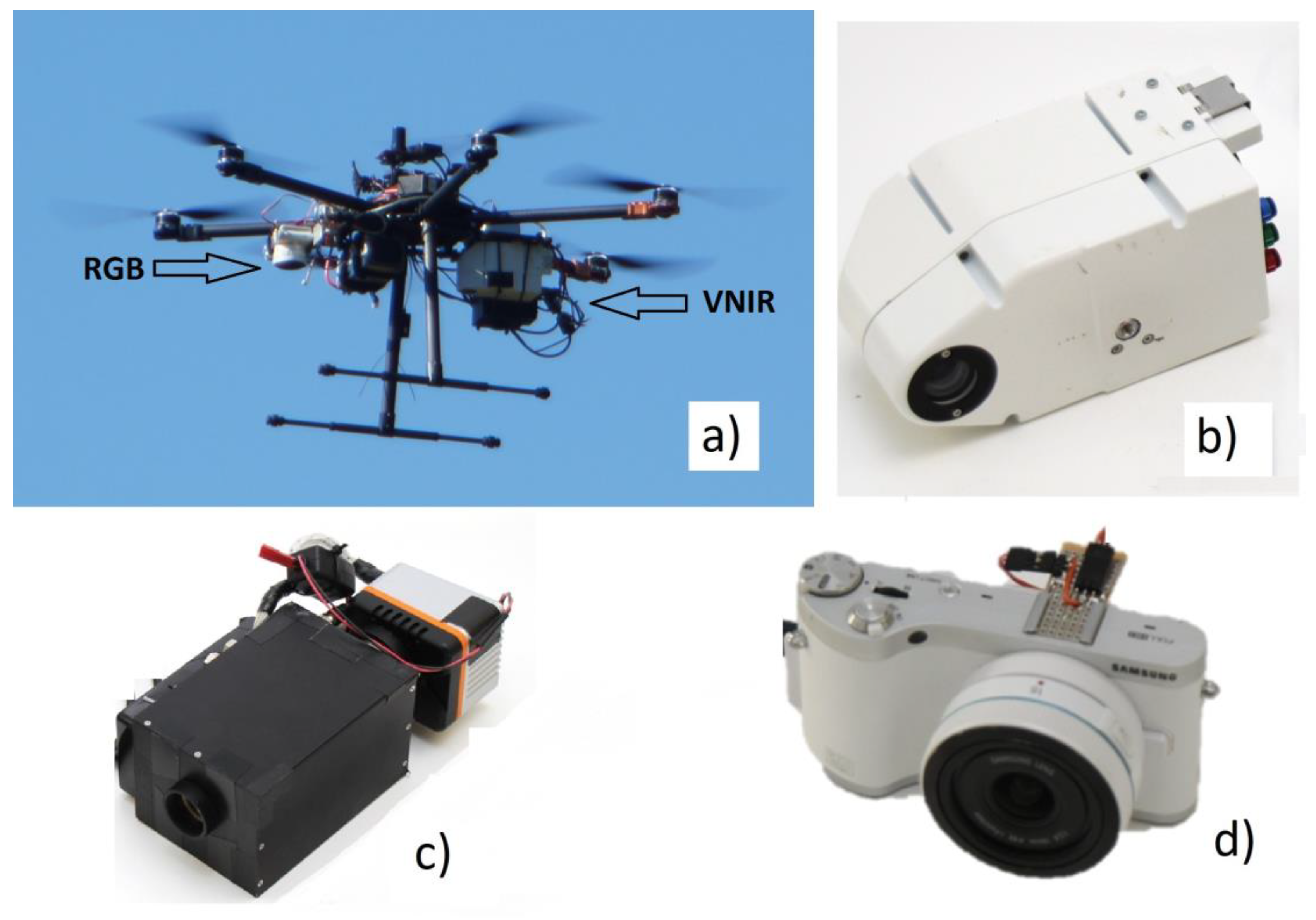
Novel HS camera technology based on a tunable Fabry-Pérot interferometer (FPI) was used in this study. The first prototypes of the FPI-based hyperspectral cameras were operating in the visible to near-infrared spectral range (500–900 nm; VNIR) [35,36,37]. The FPI camera can be easily mounted on a small UAV together with an RGB camera which enables simultaneous HS imaging with high spatial resolution photogrammetric point cloud creation. The objective of this study was to investigate the use of high resolution photogrammetric point clouds in combination with HS imagery based on two novel cameras in VNIR (400–1000 nm) and short-wavelength infrared, an SWIR (1100–1600 nm) spectral ranges in tree species recognition in an arboretum with large numbers of tree species. The effect of the applied classifier and the importance of different spectral and 3D structural features, as well as reflectance calibration for tree species classification in complex environments, were also investigated. The preliminary analysis results have been described earlier by Näsi et al. [40]. This article is an extended version of a conference paper by Tuominen et al. [23].

2. Materials and Methods

2.1. Study Area and Field Data

Mustila Arboretum, located in the municipality of Kouvola in Southeastern Finland (60°44′N, 26°25′E), was used as the study area. The area was selected for this study because it has an exceptionally large variation of tree species, mainly originating from different boreal and temperate zones of the Northern Hemisphere. Nearly 100 conifer species, and more than 200 broad-leaved tree species, have been planted there. The arboretum is over 100 years old, so a large number of fully-grown trees of various species occur in the area. Furthermore, trees of various species also form homogeneous stands, which makes the area suitable for testing tree species recognition both at the stand and individual tree level.
The total size of the arboretum is approx. 100 ha, and for this study an area of approx. 50 ha was covered by RGB and HS aerial imagery. The covered areas were selected on the basis of their tree species composition, targeting areas especially where trees composed homogeneous stands or tree groups, as well as tree species of silvicultural importance. Bushes, young trees, and trees belonging to species that do not achieve full size at maturity due to poor adaptation to Finnish conditions were excluded from the study. Furthermore, trees with canopies that were shadowed by, or intermingled with, other tree species were not included in the test material either.
Forty-seven test stands representing 26 different tree species were selected and examined in the field from the area covered by aerial imagery. From the test stands, locations of 673 test trees were recorded in the field using GPS, and the locations were marked on very high resolution RGB imagery acquired by a UAV-borne camera. The crowns of the test trees were manually delineated on the basis of the RGB imagery. The delineated trees included a number of intermingled (broadleaved) tree canopies (belonging to same species) that could not be discriminated precisely from the images. The species distribution of test tree dataset is presented in Table 1. The location of the study area and a map of the test area are presented in Figure 1.

2.2. Remote Sensing Data

2.2.1. FPI Hyperspectral Cameras

Two novel FPI-based HS cameras were used in the study. The principle of the tunable FPI technology is that the wavelength of the light passing the FPI is a function of the interferometer air gap. The final spectral response is dependent on the light passing the FPI and the spectral characteristics of the detector. Spectral bands can be selected according to the requirements of the remote sensing task. During data collection, a predefined sequence of air gap values are applied to capture the full spectral range. Since the HS data cube is formed according to the time-sequential imaging principle, the spectral bands have different positions and orientations when the camera is operated on a moving platform; this is accounted for in the post-processing phase.
A new Rikola FPI-based camera prototype manufactured by the Senop Ltd. (Kangasala, Finland) captured the VNIR range of 400–1000 nm (Figure 2b). The spectral bands could be selected with a 1 nm resolution and the number of bands was freely selectable. The full width at half maximum (FWHM) was 10–15 nm. The camera was equipped with custom optics with a focal length of 9.0 mm and an f-number of 2.8. The image size could be selected between 1010 × 648 pixels and 1010 × 1010 pixels with a pixel size of 5.5 μm. The frame rate was 30 frames/s with 15 ms exposure time for a 1010 × 648 image size. The maximum field of view (FOV) was ±18.5° in the flight and cross flight directions. The camera weighed about 720 g without a battery. The camera was operating on an independent mode saving images automatically to the compact flash card.
The SWIR camera had a spectral range of 1100–1600 nm (Figure 2c). It consisted of a commercial InGaAs camera—the Xenics Bobcat-1.7-320, imaging optics, an FPI module, control electronics, a battery, a GPS sensor, and an irradiance sensor [41]. The Xenics Bobcat-1.7-320 is an uncooled indium gallium arsenide (InGaAs) camera, with a spectral range of 900–1700 nm and 320 × 256 pixels, and with a pixel size of 20 × 20 µm. The FPI, optics, and electronics were designed and built by VTT Microelectronics (VTT). The focal length of the optics was 12.2 mm and the f-number was 3.2; the FOV was ±13° in the flight direction, ±15.5° in the cross-flight direction, and ±20° at the format corner. The time between adjacent exposures was 10 ms plus exposure time; capturing a single data cube with 32 bands and using 2 ms exposure time took 0.384 s. The mass of the spectral imager unit was approximately 1200 g. It is the first HS snapshot camera operating in the SWIR range and it was previously used by Honkavaara et al. [42] for measuring the surface moisture of a peat production area.

2.2.2. Acquisition of Remote Sensing Data

A hexacopter-type UAV with a Tarot 960 foldable frame, belonging to the Finnish Geospatial Research Institute (FGI), was used as the sensor platform in this study. The autopilot was a Pixhawk equipped with Arducopter 3.15 firmware. The payload of the system was 3–4 kg and the flight time lasted 15–30 min depending on payload, battery, and conditions. The UAV was equipped with an RGB camera + VNIR HS sensor instrumentation, as illustrated in Figure 2a.
The FPI cameras described above were the main payload on the UAV. The spectral settings of the VNIR and SWIR cameras were selected so that the spectral range was covered quite evenly (Table 2). A total of 32 spectral bands were collected by the SWIR camera in the spectral range of 1154–1578 nm with the FWHM ranging from 20 to 30 nm and with an exposure time of 2 ms. Eight SWIR bands were later rejected due to the strong water absorption, resulting in 24 usable SWIR bands (see Chapter 2.3.2). With the VNIR camera, 36 bands were collected on a spectral range of 409 nm to 973 nm with a FWHM of 10–15 nm and an exposure time of 30 ms. In addition, we also used an RGB camera (Samsung NX 300 by Samsung, Seoul, South Korea) for capturing high spatial resolution stereoscopic images which were used for producing a 3D object model using a dense image matching technique. The UAV was also equipped with an on-board NV08C-CSM L1 Global Navigation Satellite System (GNSS) receiver (NVS Navigation Technologies Ltd., Montlingen, Switzerland) for collecting the UAV position trajectory. The Raspberry Pi2 on-board computer (Raspberry Pi Foundation, Cambridge, United Kingdom) was also used for collecting timing data for all devices and for logging the GNSS receiver.
The ground station was composed of reference panels with a size of 1 m × 1 m and a nominal reflectance of 0.03, 0.09, and 0.50 for determining the reflectance transformation, and equipment for irradiance measurements. We also deployed 4–8 ground control points (GCPs) in each area with circular targets with a diameter of 30 cm. Their coordinates were measured using the virtual reference station real-time kinematic GPS (VRS-GPS) method with an accuracy of 3 cm for horizontal coordinates and 4 cm for the height [43].
The acquisition of the aerial imagery was carried out over two days on 20–21 August 2015 in three areas of interest (M1, M3, and M4; Table 3; Figure 3). Originally, one more area (M2) was included in the flight plan, but SWIR data acquisition did not materialize due to flight scheduling, and the area was left out from further analysis. The weather conditions during the flights were windless and sunny. The VNIR and SWIR cameras were operated on separate flights and the RGB camera was operated together with the HS cameras. The flying speed was 4 m/s. The flying height was 120 m at the starting position, but due to the terrain height variations and the canopy heights, the distances from the objects of interest were 70 m at the closest. Depending on the UAV-to-object distance (70–120 m) the GSDs were 0.015–0.03 m, 0.04–0.08 m, and 0.11–0.20 m for the RGB, VNIR, and SWIR cameras, respectively (Table 4). In all the blocks, the distance between the flight lines was 30 m, which resulted in side overlaps of 60% for VNIR, 50% for SWIR and 80% for RGB on the nominal flight height from the ground, and 30%, 20%, and 65%, respectively, for the highest parts of the treetops (Table 4). In Figure 4, orthomosaics of different band combinations are shown to illustrate the potential of the data.

2.3. Image Data Processing

The objectives of the data processing were to generate dense point clouds using the RGB images and to calculate image mosaics of the HS datasets. Hundreds of small-format UAV images were collected of the area of interest. The processing of FPI camera images is similar to any frame-format camera images; the major difference is the processing of the non-overlapping spectral bands. The processing chain used in this study was based on the methods developed by Honkavaara et al. [35,42,44] and Nevalainen et al. [22]:
(1)
Applying laboratory calibration corrections to the images;
(2)
Determination of the geometric imaging model, including interior and exterior orientations of the images;
(3)
Using dense image matching to create photogrammetric digital surface model (DSM);
(4)
Determination of a radiometric imaging model to transform the digital number (DNs) data to reflectance;
(5)
Calculating the HS image mosaics;
(6)
Extracting spectral and other image and 3D structural features for test trees; and
(7)
Classification of the species/genus.
In the following sections, the geometric (2, 3) and radiometric (1, 4, 5) processing steps are described. The procedures for feature extraction and classification are presented in Section 2.4 and Section 2.5.

2.3.1. Geometric Processing

Geometric processing determined the interior and exterior orientations of the images (IOP and EOP) and created sparse and dense point clouds. Since the calculating orientation of each band of the FPI data cube in the bundle block adjustment would be computationally heavy (68 bands in this study), we have developed an approach that determines the orientations of selected reference bands using block adjustment and optimizes the orientation of the remaining bands to these reference bands [44]. Agisoft PhotoScan Professional software (Agisoft LLC, St. Petersburg, Russia) was used to determine the IOPs and EOPs of the reference bands and to create 3D point clouds. The reference bands were selected so that the temporal ranges of the data cubes were covered as uniformly as possible. Four VNIR reference bands and the RGB images were processed simultaneously; in the case of SWIR data, five SWIR bands were processed simultaneously. The dataset was georeferenced using 4–8 GCPs in each area. Dense point clouds were calculated using only RGB images to acquire the highest point density and resolution. Finally, the orientations of the bands that were not processed by PhotoScan were optimized to fit to the reference bands based on the rigorous space resection method by Honkavaara et al. [44].
The block adjustments showed accurate results with re-projection errors of approximately 0.2–0.5 pixels (Table 5). The point densities were approximately 320 points/m2 for all blocks. The accuracy of geometric processing was confirmed by comparing the photogrammetric point cloud to the national airborne laser scanning (ALS) data from the National Land Survey of Finland (NLS) (Helsinki, Finland). Their differences were less than 1 m on the flat areas for most of the area. The dense point clouds were highly detailed and accurate (Figure 5a).
ALS-based digital terrain model (DTM) provided by NLS was used for converting the photogrammetric DSM to a canopy height model (CHM). The ground elevation values were extracted from DTM to each DSM point and subtracted from the point’s Z coordinate value, resulting in the height above ground.

2.3.2. Radiometric Processing

The objective of the radiometric preprocessing was to provide spectrally high-quality reflectance mosaics. The radiometric modelling approach developed at the FGI includes sensor corrections, atmospheric correction, correction for the radiometric nonuniformities due to illumination changes and other effects, and the normalization of the object reflectance anisotropy related non-uniformities using bidirectional reflectance distribution function (BRDF) correction [35].
The sensor corrections for the FPI images included dark signal correction and photon response non-uniformity correction (PRNU) [35,36]. The dark signal correction was calculated using a black image collected immediately before the data capture with a covered lens and the PRNU correction was determined in the laboratory. In this investigation, both corrections were used for the VNIR datasets and, for the SWIR datasets, only the dark signal correction was used. The resulting datasets are referred to as DN images in this study.
The reflectance calibration to convert the DNs to reflectance were carried out using the empirical line method [45] with the aid of the reflectance panels in the area. For the SWIR images, all reflectance panels were used (nominal reflectance 0.03, 0.10, and 0.5). For the VNIR images, the brightest panel was not used because it was saturated in most of the bands.
The illumination conditions were sunny and uniform, thus, object anisotropy effects could cause radiometric disturbance in the mosaics. The view zenith angles in each mosaic point were mostly less than ±10°; the largest view zenith angle differences of up to ±20° appeared in mosaic seams between the adjacent flight lines (Figure 5b). The flight plan in the majority of the flights was such that the solar principal plane direction was close to the direction of the flight and, thus, the most significant anisotropy effects that occurred in the principal plane in the backward and forward scattering directions appeared between adjacent images within flight lines with smaller than 3° view zenith angles, which minimized the anisotropy effects. Furthermore, tree crowns can be considered rough objects with large natural reflectance variations, which might exceed the anisotropy effects with small view zenith angles. As we could not observe any anisotropy effects when visually evaluating the mosaics we decided not to use anisotropy correction during the mosaicking. The illumination conditions were uniform throughout the flights and so additional radiometric corrections were not necessary.
The DN and reflectance orthophoto mosaics were calculated with a GSD of 20 cm utilizing most nadir parts of the images using the FGI’s radiometric block adjustment and mosaicking software [35]. Eight bands in the SWIR data in the range of 1360–1470 nm were unusable due to the low signal level because of the strong water absorption in this spectral range. The resulting reflectance mosaics had good radiometric qualities. The band registration quality was evaluated visually, and the discrepancies were mostly less than one pixel.

2.4. Extraction of Spectral and 3D Features

Spectral and 3D features were extracted from delineated polygons corresponding to the canopies of test trees in the study area. The CHM was applied in the extraction process to ensure that the spectral features of the HS VNIR and SWIR, as well as RGB imagery, were extracted from the crowns of the test trees and to exclude the influence of the ground vegetation and shrubs on the image features. Pixels whose altitude was lower than 5 m from the terrain level were excluded from the calculation of the spectral features.
Spectral features were extracted from:
(1)
Thirty-six VNIR and 24 SWIR spectral bands with both digital number (DN) and reflectance values;
(2)
The first 9 and 12 principal components (PC) calculated from the VNIR and SWIR DN bands, respectively;
(3)
The first 17 and 15 PCs calculated from the VNIR and SWIR reflectance bands, respectively; and
(4)
Three bands of RGB imagery.
The following spectral features were extracted from the datasets listed above:
(1)
Spectral averages (AVG);
(2)
Standard deviations (STD);
(3)
Spectral averages (AVG50) of the brightest 50% of the pixel values; and
(4)
Spectral averages (AVG25) of the brightest 25% of the pixel values,
The following features were extracted from photogrammetric CHM (3D point data) [46,47,48]:
(1)
H, where the percentages of vegetation points (0%, 5%, 10%, 20%, …, 80%, 85%,90%, 95%, 100%) were accumulated [m] (e.g., H0, H05, ..., H95, H100);
(2)
Canopy densities corresponding to the proportion of points above the fraction nos. 0, 1, …, 9 to the total number of points (D0, D1, …, D9); and
(3)
The proportion of vegetation points with an H greater or equal to the corresponding percentile of H (i.e., P20 is the proportion of points where H ≥ H20) (%)*; where H = height above ground; vegetation point = point with H ≥ 2 m (* the range of H was divided into 10 fractions (0, 1, 2, …, 9) of equal distance).

2.5. Feature Selection and Classification of Tree Species

RGB features were used to set a reference value for the HS data in tree species classification. In total, 24 spectral features were extracted from RGB imagery (12 DN and 12 reflectance features). The features extracted from the HS imagery encompassed a total of 368 reflectance features and 324 DN features (the disparity is due to the different number of PCs applied). The number of 3D CHM features was 29. All spectral and point features were scaled to a standard deviation of 1. This was done because the original RS features had very diverse scales of variation. Without scaling, variables with wide variation would have had greater weight in the estimation, regardless of their capability for estimating the forest attributes.
Feature selection was carried out for 14 sets of features: SWIR, VNIR, SWIR+VNIR, RGB+3D, SWIR+3D, VNIR+3D, SWIR+VNIR+3D extracted from the DN and reflectance mosaics. The extracted feature sets were large, presenting a very high-dimensional feature space. In order to avoid the problems of a high-dimensional feature space, i.e., the “curse of dimensionality”, which is inclined to complicate the classification procedure [49,50], the dimensionality of the data was reduced by selecting a subset of features aiming to achieve good discrimination ability.
Two alternative methods were used for the feature selection and tree species and genus prediction: (1) the k-nearest neighbor classifier in combination with a genetic algorithm-based feature selection and (2) the random forest method.

2.5.1. The k-Nearest Neighbor Method (k-nn)

In the k-nn method [51,52,53] the Euclidean distances between the test trees were calculated in the n-dimensional feature space, where n stands for the total number of remote sensing features used. The tree species/genus was estimated for each test tree as the statistical mode of the nearest neighbors (i.e., the most common species/genus among the nearest neighbors). Different values of k were tested in the estimation procedure.
The accuracy of the tree species estimation was tested by calculating error matrices, e.g., [54] for the tested classifications. The error matrix presents the error of omission (observations belonging to a certain category and erroneously classified in another category), error of commission (observations erroneously classified in a certain category while belonging to another), proportion of observations classified correctly, and the kappa (κ) value.
Whereas the proportion of correct classifications is a generally used measure of estimation accuracy in the case of categorical variables, in certain situations it may be high even though the classification is not very good, e.g., in the case where a high proportion of the observed values belong to a single category. Kappa (κ) is a statistical measure, which indicates the success of the classification relative to a random assignment of the observations to categories. A general definition of kappa is given in Equation (1):
κ = p 0 p e 1 p e
where p0 is the proportion of correct estimates and pe is the proportion of correct estimates in a random classification. The kappa value has range of 0–1, where value 0 indicates a fully-random classification and 1 a perfect classification.
The selection of the features was performed using a genetic algorithm (GA)-based approach, implemented in the R language by means of the Genalg package [55,56]. This method searches for a subset of predictor variables based on a criteria defined by the user. Although there is no guarantee of finding the optimal predictor variable subset [57], and the algorithm does not go through all the possible combinations, solutions close to optimal can usually be found in a feasible computational time. Here, the objective function imposed for GA was to maximize the proportion of correct classifications. The general GA procedure has been described in [58,59], and a more detailed description of the GA algorithm applied in this study is presented in Tuominen et al. [60]. In the selection procedure, the population consisted of 100 binary chromosomes, and the number of generations was 40. We carried out 10 feature-selection runs with each dataset to find the feature combination that returned the best evaluation value. The optimal value for parameter k was selected during test runs for each tested feature set. The selected number of nearest neighbors was 3 and the weight for inverse distance weighting was 1 for all feature sets.

2.5.2. Random Forest Method (RF)

The RF method is based on growing multiple decision trees. A decision tree is used to create a model that predicts the value of a target variable based on a set of input variables. As with GA, the target variables were tree species and genera, while the input variables were the features extracted from the HS and 3D datasets. Each internal node in a tree corresponds to a test on one of the features. Each branch represents a series of tests and at the end of each branch the terminal node represents the outcome of the tests, which is a value for the target variable. The tree votes for the mode of all the values at the terminal nodes. In the case of equal values the final estimate is selected randomly [61].
Single decision trees are prone to overfitting, but by growing an adequate number of trees this disadvantage can be eliminated or minimized. In order to be able to grow different decision trees some source of randomness is required. The first is to randomly subsample the training data. The second is to subset the number of features used for each node in each decision tree [62].
The data analysis for this study was carried out using the randomForest package in the R statistical software package [55]. After several test runs the default number of 500 decision trees to be grown for each data set (see Section 2.4) was found to be suitable. At each node a random set of features were used. The optimal sample size of the features for each dataset was selected from test runs with sample sizes varying from 10 to 70 with an increment of 5. Subsampling of the training data was done by replacement and the size of the subsample equaled the size of the training data. One-hundred runs were carried out with each dataset and the best-performing model was selected. The fitness of the model was assessed by the overall accuracy of the target variables (tree species, genera).

3. Results

3.1. Spectral and 3D Data

We evaluated the separability of species based on the average spectral data. We calculated average spectra of the brightest 50% of canopy pixels for deciduous tree species and evergreen tree species (Figure 6). In the visible spectral range (approx. 400–700 nm) there was very little difference between the reflectance values of the tested tree species, only Abies mariesii had slightly higher reflectance values compared to other tree species. Furthermore, the reflectance of band with central wavelength of 409 and 973 nm (short edge of VNIR) appeared to contain artefacts (not plotted). The discrimination between tree species was most pronounced in the near-infrared range and in the short end of SWIR (approx. 700–1300 nm). In the SWIR range from 1300 nm the discrimination capability of the reflectance values again fell markedly, also due to missing channels in the strong water absorption range of 1360–1470 nm. With longer wavelengths the differences between the reflectance values of tree species again became more distinct (from 1470 to approx. 1600 nm).
Selected examples of point clouds of tree species and genera are illustrated in Appendix A in Figure A1 (evergreen coniferous genera) and Figure A2 (deciduous genera). 3D representations of the point clouds that can be observed from different angles are presented in supplementary data (as HTML-files). These point clouds show some species specific features, which could support the tree species classification. For example, regarding the evergreen conifers, the Pseudotsuga sp. and Tsuga sp. had sharper crown than Thuja sp. and Pinus sp. In the cases of the deciduous genera, the Acer and Tilia sp. had much wider and flatter crowns than Populus sp. and Quercus sp.

3.2. Classification Results

The quantitative results of tree species and genus classifications based on different combinations of HS imagery (original DN values) and 3D data using k-nn+GA classifier are presented in Figure 7a, and similar results using the RF classifier are presented in Figure 7b. The results based on calibrated reflectances of HS bands and 3D data are presented in Figure 8a (k-nn+GA classifier) and Figure 8b (RF classifier). The proportion of correct classes as well as the kappa coefficients are presented for each combination of input data in Figure 7a,b and Figure 8a,b.
When testing the different spectral band combinations of the original DNs with and without 3D point cloud data in the classification of tree species and genus, the relative performances of the tested data sources were quite similar, regardless of the classifier applied (see Figure 7a,b). The original SWIR bands alone were the poorest performing HS data source; the percentage of correct classifications was 59% when using the GA classifier and 60% when using the RF classifier for tree species, and 69% (GA) and 68% (RF) for the tree genus. Using VNIR bands generally improved the accuracy for tree species 12–14% (depending on the classifier) and the accuracy for the genus 7–12%, compared to the SWIR alone. The combination of SWIR+VNIR bands resulted in an improvement of 0–7% for tree species classification (depending on the classifier) and 1–5% for genus classification, compared to the VNIR bands only. The reference classification by 3D+RGB features resulted in generally similar accuracy as SWIR (without 3D).
The inclusion of 3D point cloud data markedly improved the classification accuracy without exception. The accuracy improvement brought by the inclusion of 3D data was 16–23% (for the species) and 7–15% (for the genus) when using 3D+SWIR; 9–15% (for the species) and 6–8% (for the genus) using 3D+VNIR; and 11% (for the species) and 4–6% (for the genus) when using a combination of 3D+SWIR+VNIR. Thus, the best performing data combination for both species and genus was the 3D+SWIR+VNIR combination, but in the genus classification, the improvement compared to classification by 3D+VNIR was quite small.
Compared to species and genus classifications based on original pixel DNs, the reflectance calibration resulted in a significant improvement for both species and genus classifications (see Figure 8a,b). The use of calibrated reflectance values improved the tree species classification accuracy 9–12% with the SWIR data, 4–7% with the VNIR data, and 5–7% with the SWIR+VNIR data. The improvement in the species classification using calibrated reflectance values was smaller when 3D data was also included: 5–6% with 3D+SWIR, 1–4% with 3D+VNIR, and 2–5% with 3D+SWIR+VNIR. In the tree genus classification, the trend and level of improvement was similar to the species classification; i.e., the use of calibrated reflectance values always improved the genus classification accuracy, regardless of the classifier applied or the HS band combination used. Additionally, for 3D+RGB reflectance calibration improved the accuracy 5–6% for species and 7% for genus classification.
When comparing the classifiers, the k-nn (applied with GA) gave consistently better results than the RF method in selecting feature sets for classification (Figure 7a,b and Figure 8a,b). The results from k-nn+GA were better than RF both in the recognition of tree species and tree genus and, furthermore, k-nn+GA performed better with all the tested HS and 3D data combinations. When predicting tree species (using calibrated reflectance values), the accuracy (measured by the proportion of correct classifications) via k-nn+GA was 3% higher than RF with SWIR, 4% higher with VNIR, 5% higher with SWIR+VNIR, 4% higher with 3D+SWIR, 3% higher with 3D+VNIR, and 5% higher with 3D+SWIR+VNIR. When predicting the tree genus, the accuracy of k-nn+GA was improved by 4% (both SWIR and VNIR), 5% (SWIR+VNIR), 7% (3D+SWIR), 4% (3D+VNIR), and 7% (3D+SWIR+VNIR) compared to the accuracy of RF. The only exception was 3D+RGB where RF brought similar or slightly better accuracy than k-nn+GA; 3% higher for species and similar accuracy for genus.
Thus, the best classification results were achieved by using calibrated reflectance values of HS bands, applying k-nn+GA as classifier, and using 3D features in combination with both SWIR and VNIR bands. When the κ coefficients of alternative species and genus classifications were examined, most classifications indicated substantial agreement between the observed and estimated classes (0.6 < κ ≤ 0.8). Only the use of original DN values for SWIR bands resulted in κ less than 0.6, which indicates only moderate agreement between the observed and estimated species/genus classes. The best performing feature combinations containing 3D+SWIR+VNIR data typically resulted in κ higher than 0.8, when applied with a k-nn+GA classifier, indicating almost perfect agreement between observed and estimated species/genus classes.
When examining the recognition of tree genus (see Figure 9a) with the best performing classifier (i.e., k-nn+GA) and the best combination of 3D data and HS imagery (i.e., calibrated reflectances of SWIR+VNIR bands), the coniferous trees of the different genera were typically well discriminated from each other; the user’s and producer’s accuracy for individual genera was typically well over 0.7, with the exception of Pseudotsuga sp. and Abies sp., which were quite often confused. 3D data typically slightly improved their recognition. Genus Larix was generally recognized to a high degree of accuracy, but in the cases when classified incorrectly it was confused with broadleaved genera. Broadleaved trees of different genera were typically more difficult to distinguish from each other, and the accuracies of different genera fluctuated widely: the user’s and producer’s accuracies are mainly between 0.5–0.9. Additionally, for broadleaved trees the inclusion of 3D data generally improved the genus recognition, but also the opposite result occurred between certain genera (e.g., Tilia sp.).
When examining the tree species recognition (Figure 9b) using k-nn+GA and 3D+SWIR+VNIR reflectances, coniferous trees were often confused with other tree species of the same genera (especially within genera Abies and Picea), and their species level recognition accuracy was considerably lower than for the level of tree genera. Most broadleaved tree genera usually had only one species represented in the test material and, thus, the results per tree species were quite similar as the per genera results. The user’s and producer’s accuracies per class are presented in Figure 9a (per tree genus) and Figure 9b (by tree species).
The number of features selected from each RS data source (3D, SWIR, and VNIR) in the best classifications are presented in Table 6. Numbers of both reflectance and DN HS features are given. Furthermore, the full confusion matrix for the tree genus classification is presented in Table 7.

4. Discussion

The combination of HS bands over a wide spectral range and 3D features from point cloud data allows the extraction of a very high number of remote sensing features for the classification task. As a consequence, the classification task is carried out in a high-dimensional feature space. As the dimensionality grows, all data typically become sparse in relation to the dimensions [50], which causes problems for classifiers based on the distance or proximity in the feature space, such as k-nn, e.g., [49]. In hyper-dimensional feature space, the distances from any point to its nearest and farthest neighbors tend to become similar [49], which makes it questionable whether the nearest neighbors found are the true nearest neighbors. Therefore, the number of remote sensing features must be reduced for producing an appropriate subset of features for the classification task considering their usefulness in recognizing the classes, as well as their mutual correlation. In recent forest estimation and classification studies various algorithms have been applied for this purpose [
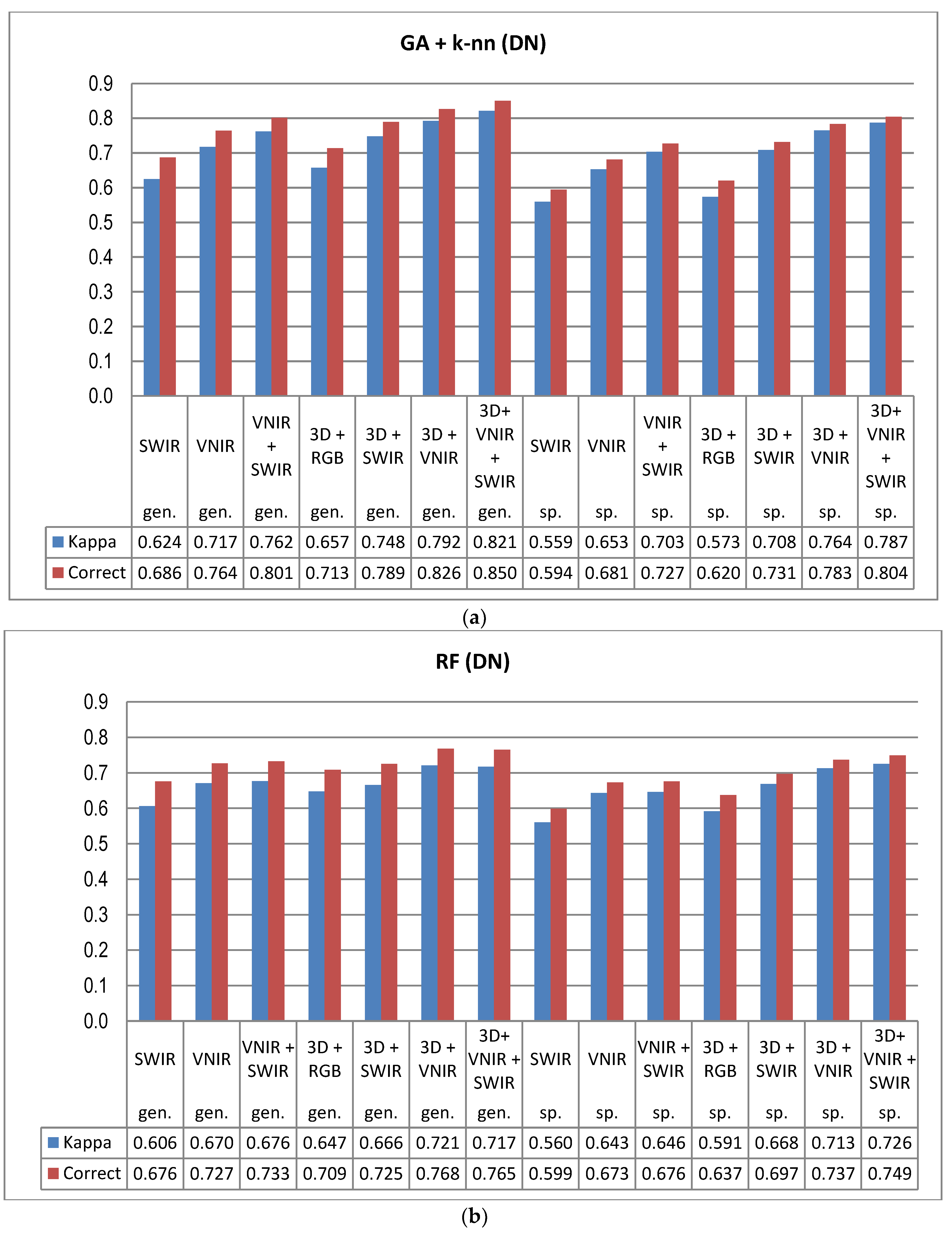
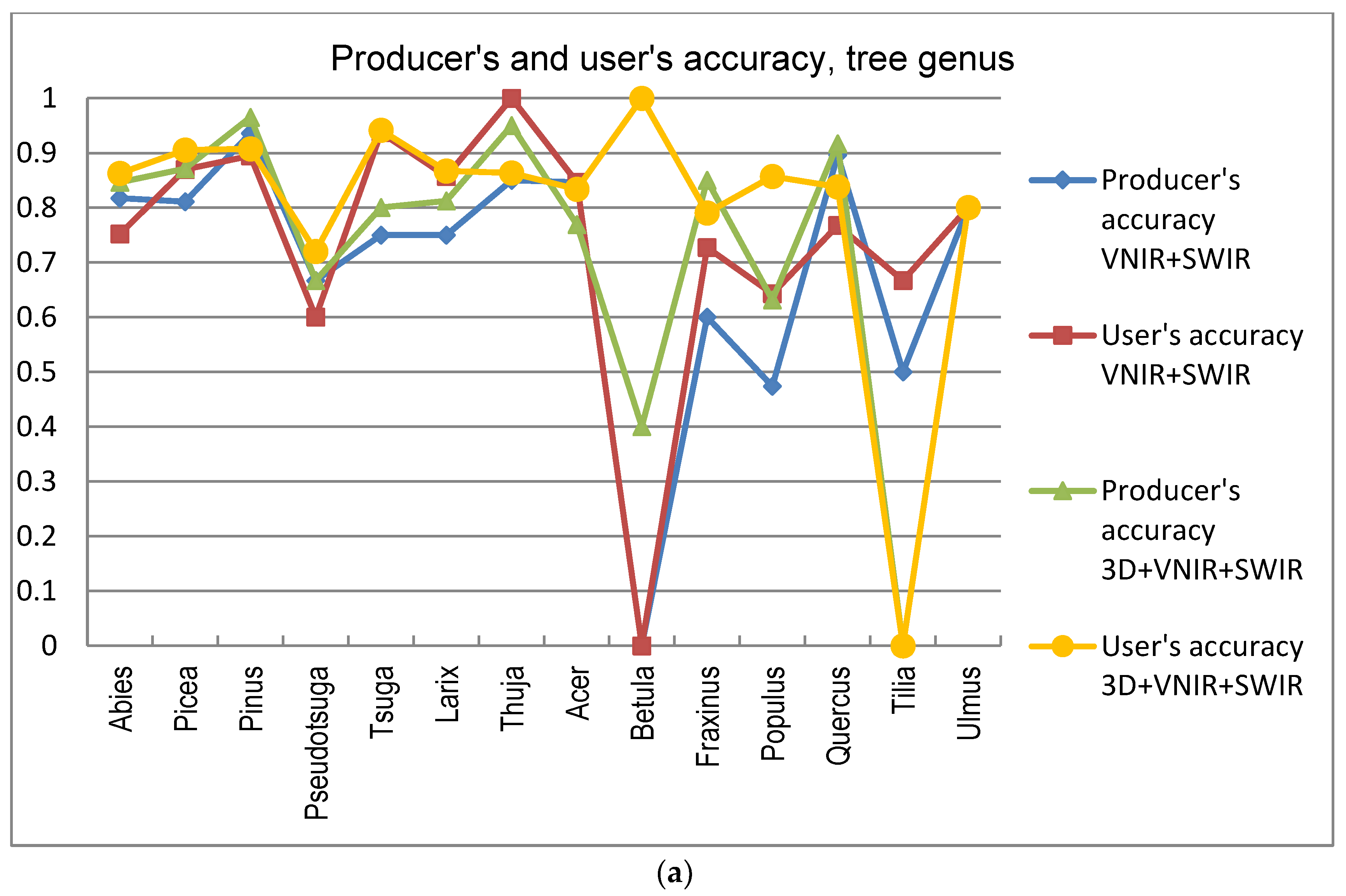
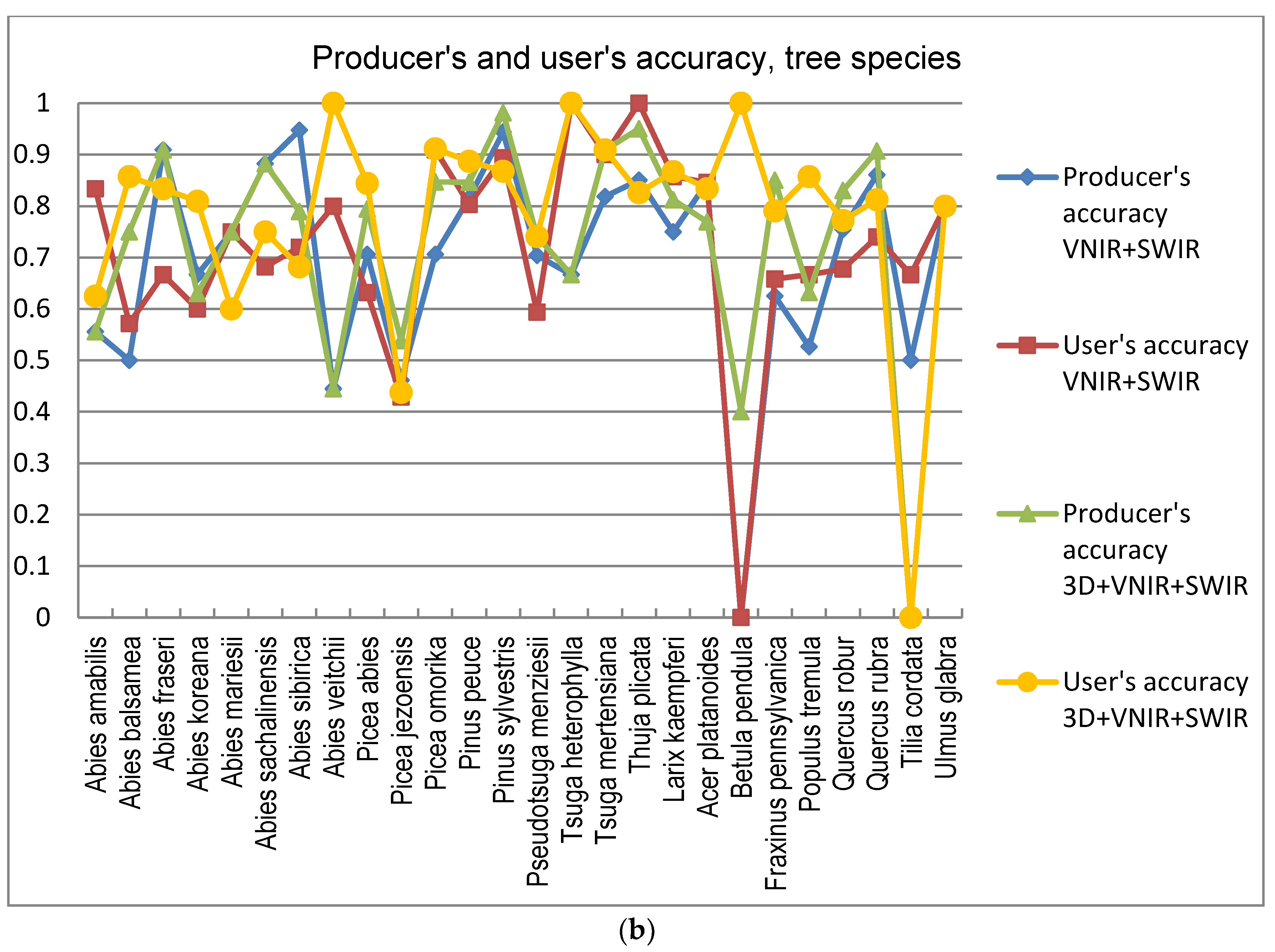
5]. In this study the GA procedure used in combination with a k-nn classifier provided otherwise consistently better results in tree species and genus recognition than RF, with the exception of 3D+RGB (the dataset having the lowest number of features) where RF performed slightly better. Thus, the GA algorithm applied here was found to be a viable tool for finding an appropriate set of features for this task, especially in a very high-dimensional feature space, such as that tested in this study. Both classification methods applied in this study have feature selection components which are stochastic by nature, which means that there is a random effect in their results. This effect was apparent especially in those tree species which had few test trees, and the user’s and producer’s accuracy of these species varied highly between 0–1 with different feature combinations (see Figure 9a,b).
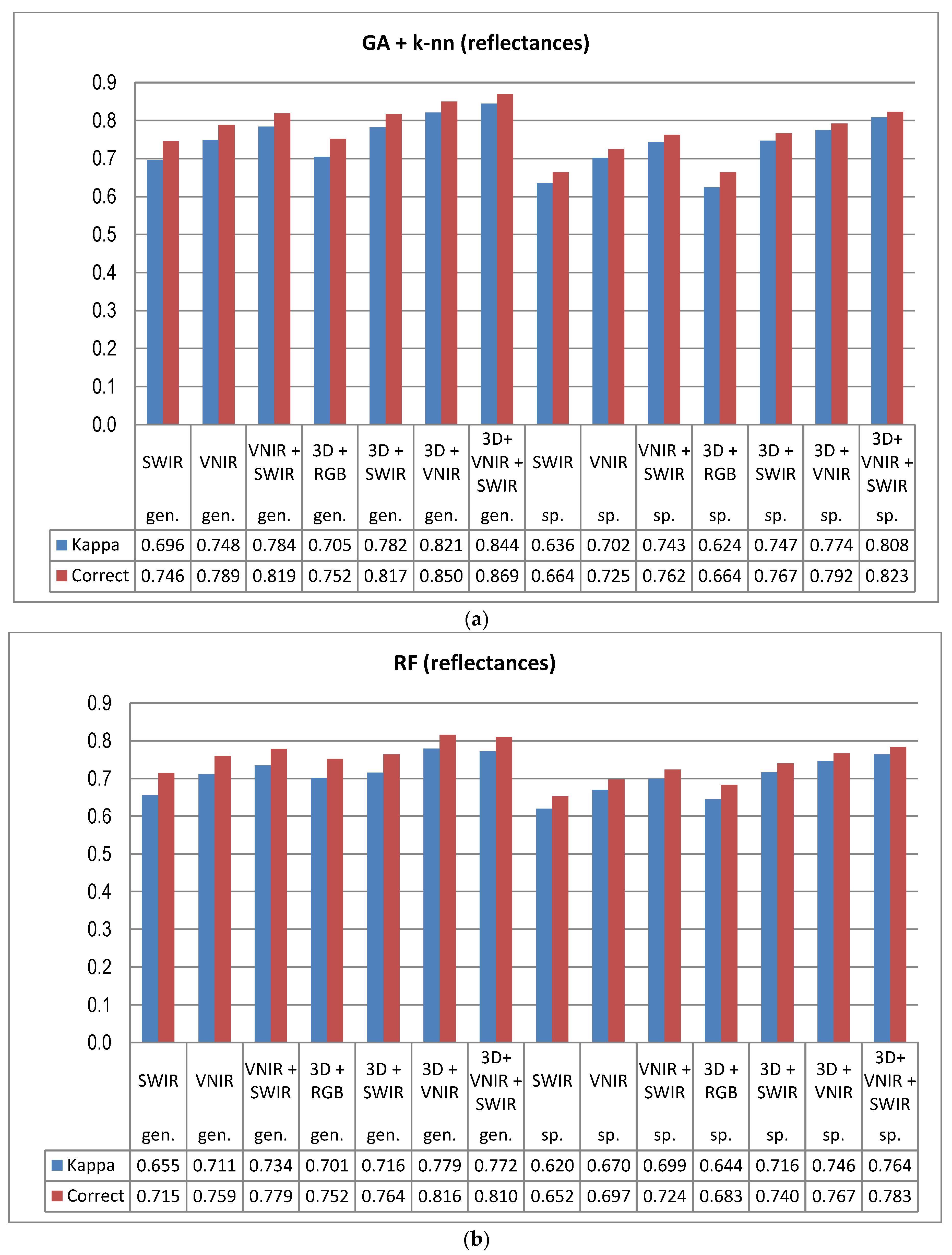
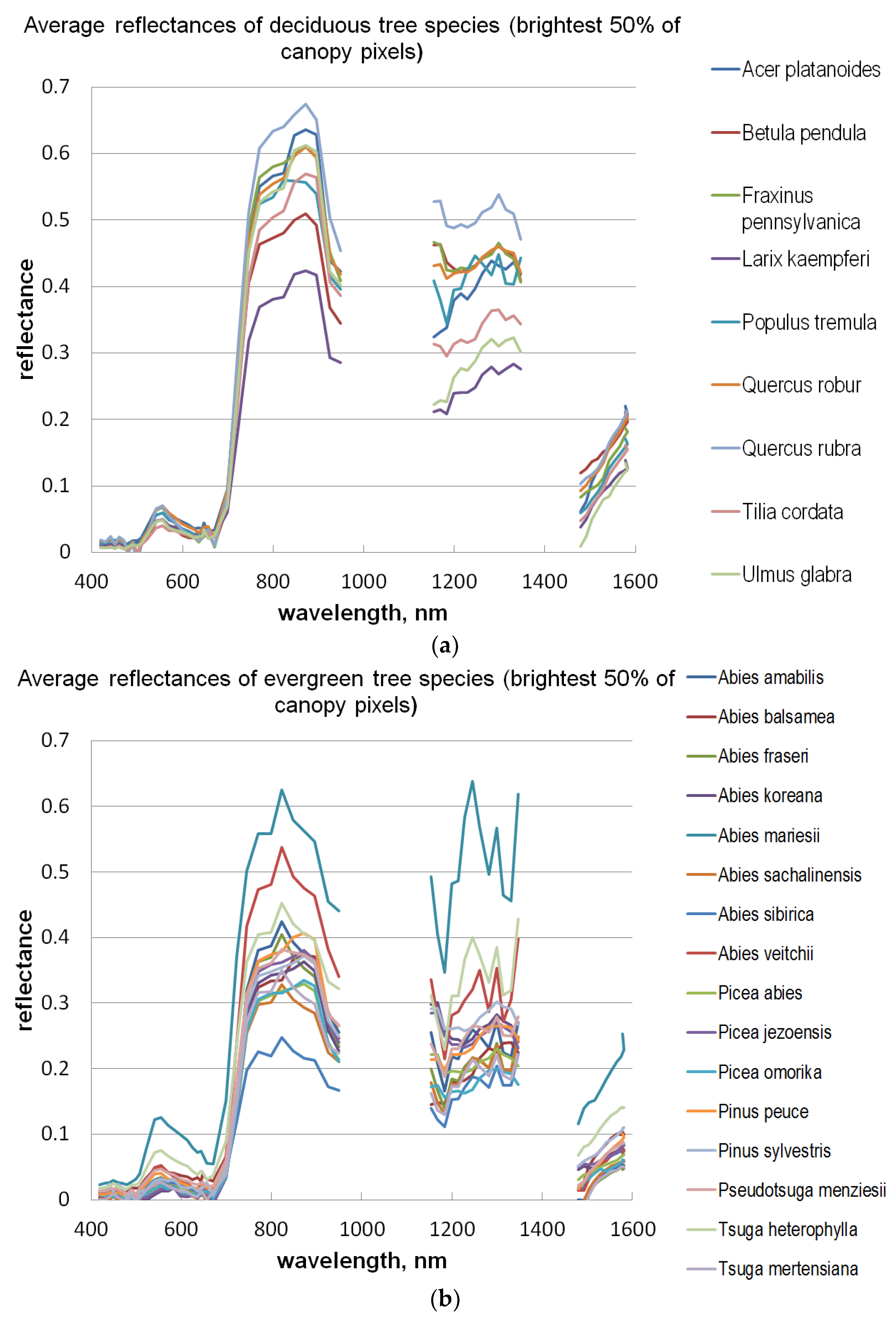
Another main finding of this study was the significance of the calibration of the HS imagery for tree species recognition. Compared to pixel DN values that were disturbed according to the variations in the illumination levels and sensor characteristics, the calibrated reflectance consistently provided better results in tree species and genus recognition, and this trend was similar across all the spectral band combinations tested here. Although the HS image acquisition was carried out in clear sunny weather conditions, it was necessary to compensate for the illumination changes caused by varying solar elevation over the 5–6 h of data capture each day. We used the empirical line method to carry out the calibration. In UAV campaigns, there are always variations in pixel values that are caused by other factors than the properties of the target of observation (i.e., tree canopies), such as changing illumination by solar elevation and azimuth angles, as well as object reflectance anisotropy effects or illumination changes due to clouds, which necessitate, in most cases, the use of advanced methods for image calibration in order to be able to utilize the full potential of HS imagery. The radiometric block adjustment is an example of such a method [22,35,39].
Despite the high spectral and radiometric resolution of the HS imagery applied, the inclusion of 3D features extracted from point cloud data of the stereo-photogrammetric canopy surface model always improved the accuracy of tree species recognition. The dataset having the least spectral information (i.e., 3D+RGB) generally resulted in similar accuracy as the poorest performing HS data (SWIR) without 3D. To a certain extent, the effect of reflectance calibration and 3D features was also complementary; when original pixel values were applied, the effect of 3D features was more prominent than with calibrated reflectances and the use of calibrated reflectances had smaller effects on the accuracy when the classification was based on data combinations that included 3D features. It is possible that the calibration could have resulted in even greater improvements to the results, if the weather had been more variable [23]. In operational forest inventories the significance of 3D data is typically considerably higher, since there are many other variables of importance, such as the volume of growing stock and the amount of biomass, as well as variables related to the size of the trees, e.g., stand mean diameter and height, where 3D data is a key factor in their accurate prediction. Based on our results, the SWIR-range data did not provide advantages for the classification, thus VNIR-hyperspectral data was sufficient. The approach integrating spectral and 3D features has significant potential to develop a high-performing automatic classifier.
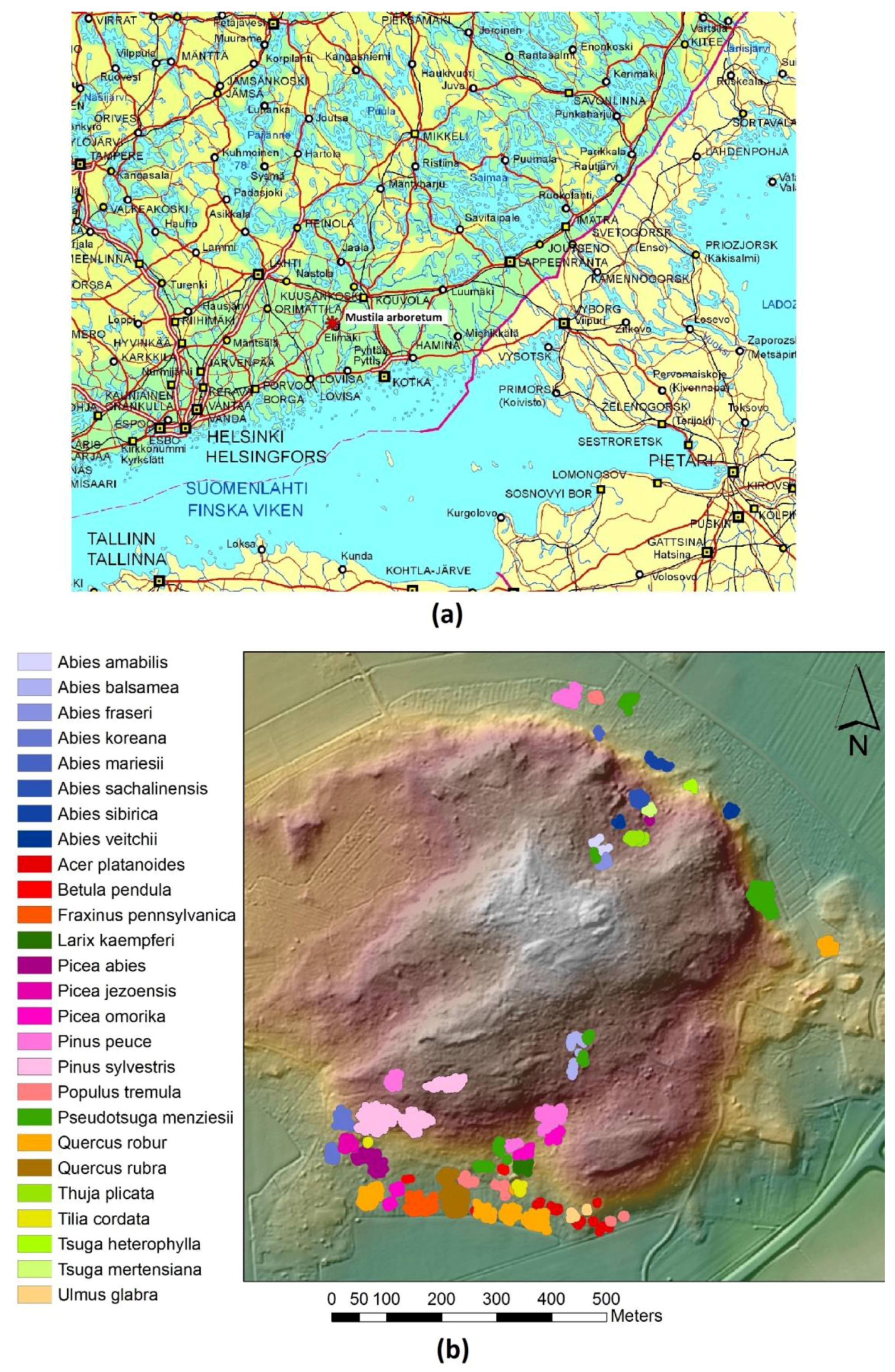
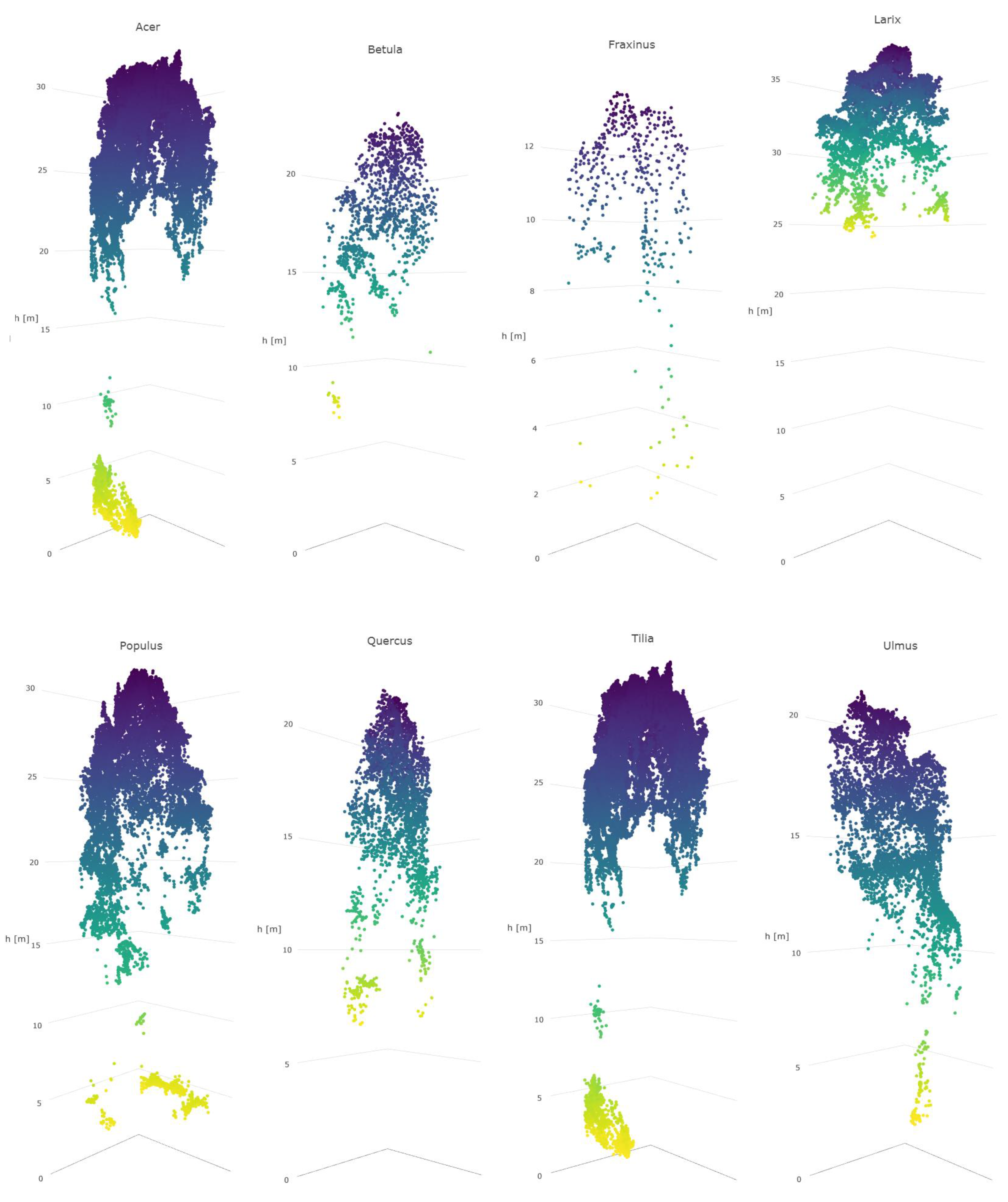
A number of broadleaved tree species that occur naturally primarily in the temperate vegetation zone and in the study area are on the northern edge of the distribution map, such as Tilia cordata, Ulmus glabra, Acer platanoides, and 
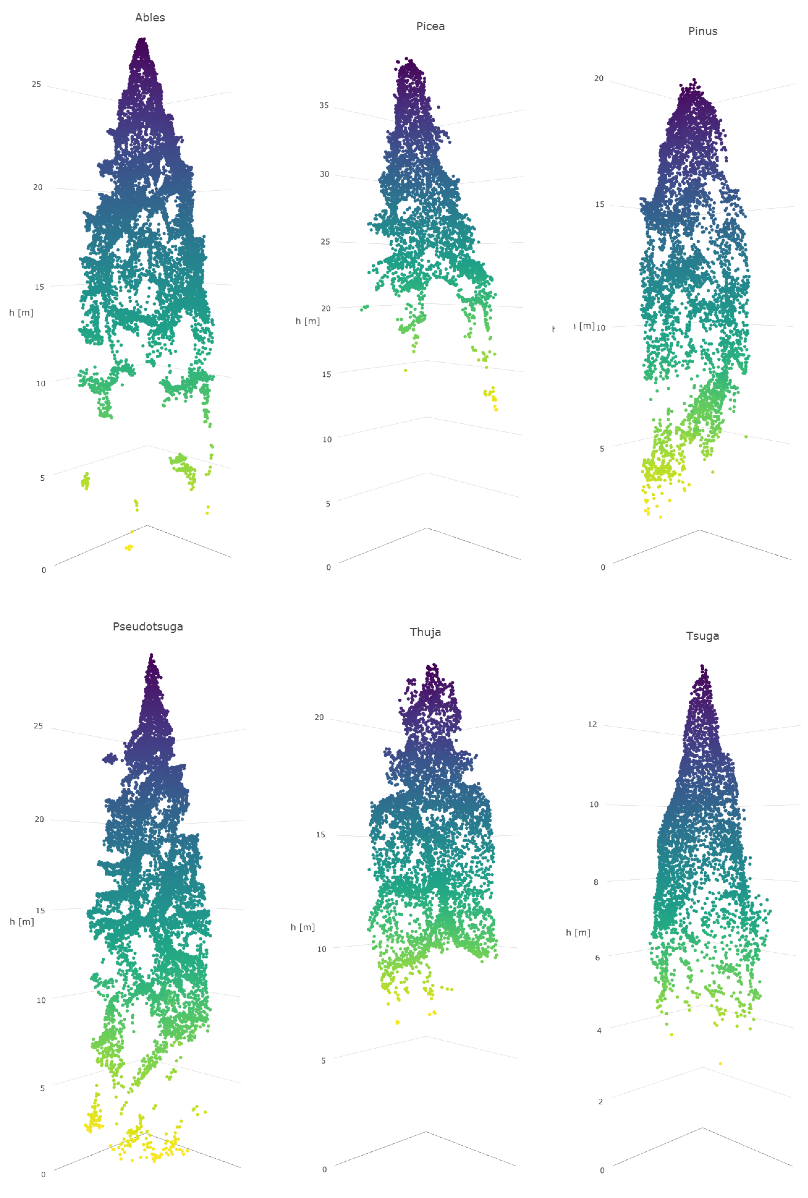
Quercus sp., are difficult to distinguish from each other, even with a combination of HS and 3D data. Apparently, their spectral properties, as well as the geometric shape of the canopy, seem to resemble each other (see Figure 8). Additionally, the classification of Betula had a very low level of accuracy, and it was often confused with other broadleaved trees. This is somewhat contrary to expectations, since the leaves of Betula sp. somewhat differ from other broadleaved trees in the test material. The poor accuracy of these species may be partly because some of these species had a low number of trees in the test data.
Trees belonging to Larix sp. which, botanically, are classified as conifers, have spectral characteristics mainly resembling broadleaved trees, due to the properties of their needles, e.g., [63]. Here, also, Larix sp. trees were partly confused with broadleaved trees, which was otherwise rare for other coniferous trees. Trees belonging to
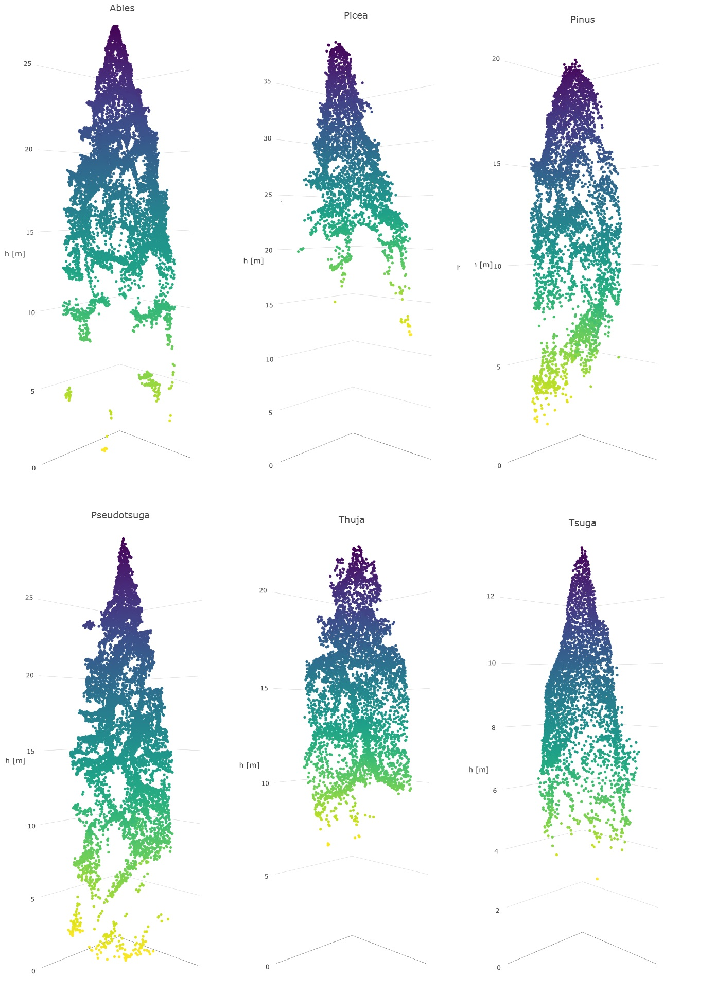
 Abies sp., Picea sp., Pseudotsuga sp., and Tsuga sp. were sometimes difficult to distinguish from each other due to the similar physical appearance of their canopies in the 3D data. Furthermore, in the classification on the individual tree species level, members of Abies sp. were often confused with each other, due to their similarity even when observed in the field. Of all the tree genera, Thuja sp. (only one species included in the study material, Thuja plicata) had the highest producer’s level of accuracy, which was intuitively foreseen since Thuja sp. has a peculiar needle form, which apparently can be clearly distinguished by HS bands. This was obvious since the classification accuracy of Thuja sp. is high even when HS bands are used without 3D data. In addition, also the canopy form of Thuja sp. was somewhat unique among the test trees.
In this study we used test material, where trees formed stands or tree groups that showed homogeneous species composition. In natural forests, however, canopies of different species are often intermingled with each other, causing further complication for individual tree-level recognition, whose effect was not studied here. Due to the selection of the test material, a similar level of accuracy may not be achieved in operational forest inventories where the target forests are often mixed.
Most previous studies concerning tree species classification using the UAV-based (as well as other airborne) datasets have been carried out in forests with less-diverse species structure. Generally, in studies concerning Nordic conditions there are few tree species present [14]. Nevalainen et al. [19] used an FPI camera operating in the wavelength range of 500–900 nm in the classification of five species in a boreal forest. The best results were obtained with RF and multilayer perceptron (MLP), which both gave 95% overall accuracies and kappa values of 0.90–0.91. Our analysis in the study area of higher species diversity did not reach as high an accuracy, but also the task was more complex. In Norwegian boreal forest conditions Dalponte et al. [13] have used ALS and hyperspectral data for separating pine, spruce, and broadleaved species using support vector machines, achieving overall accuracies as high as of 93.5% and kappa values of 0.89 for those three species. Dalponte et al. [13] have noted that using automatic tree delineation instead of manual delineation lowered the accuracy markedly. We delineated tree crowns manually for this study in order to focus on the performance of the input data and classifiers. In operational applications automatic delineation of tree crowns should be applied, which brings an additional source of potential errors in species recognition. Thus, for an operational application, the results of this study may give too optimistic an impression.
In studies applying more diverse species material the level of accuracy similar to this study have been reported by, e.g., Zhang and Hu [15], who achieved an overall accuracy of 86.1% and kappa coefficient of 0.826 using a combination of spectral, textural, and longitudinal crown profile features extracted from high-resolution multispectral imagery. However, their test material covered only six tree species from an urban environment. Zhang and Hu [15] argue that the shape of trees is likely to be more species-specific in urban areas (due to lower competition) than in forests. Waser et al. [12] have used LiDAR in combination with RGB and CIR imagery in an alpine forest, achieving overall accuracies between 0.76 and 0.83, and kappa values between 0.70 and 0.73 with multinomial regression models. The test data of Waser et al. [12]. consisted of nine tree species. Ballanti et al. [64]. have tested combination of LiDAR and hyperspectral imagery in the Western USA using support vector machines and RF as classifiers, achieving accuracies between 91 and 95%, their test data consisted of eight tree species with a relatively wide range of physiological characteristics.
Accurate tree species recognition was achieved by Kim et al. [65] with test material of even higher species diversity (15 species) using LiDAR data, but their best recognition (over 90%) was achieved by combining LiDAR data from both leaf-on and leaf-off seasons. However, with single-season data, the species recognition accuracy was approx. 80%, and the leaf-off data performed markedly better than data from the leaf-on season [65]. Kim et al. [65] have especially noted the capability of LiDAR intensity values from different seasons to distinguish various tree species. Zhang and Qiu [66] have used a combination of LiDAR data and hyperspectral imagery for species recognition in test material of even higher species diversity (40 species), achieving an accuracy of 68.8% and a kappa value of 0.66. Aforementioned studies have used conventional aircraft as sensor platforms and, thus, applied somewhat lower spatial resolution data than this study.
It is highly likely that further improvement in species recognition accuracy can be achieved by utilizing multitemporal data in the classification process. For example, Somers and Asner [67] found the phenology to be key to spectral separability analysis when using low spatial-resolution Hyperion data. Similar findings were made by Kim et al. [65] using LiDAR data and Mickelson et al. [68] using optical satellite imagery.

5. Conclusions

Our study was the first one to develop and assess UAV-based 3D hyperspectral remote sensing datasets for species classification at the individual tree level for a forest having high species diversity. We used two novel miniaturized 2D-format hyperspectral cameras operating in the visible to near-infrared (VNIR; 400–1000 nm) and shortwave infrared (SWIR; 1100–1600 nm) ranges. In addition, we utilized a canopy height model created utilizing a photogrammetric dense surface model to extract 3D structural features. The tested feature combinations were able to predict the tree species and genus accurately in a diverse set of field data. Our results showed that the most accurate tree species recognition was achieved with the combination of spectral features from the VNIR and SWIR imagery together with features from photogrammetric 3D point cloud data. The proportion of correctly classified trees was 0.823 for tree species and 0.869 for tree genera; the corresponding kappa factors were 0.808 and 0.844, respectively. The next best results were nearly as good, and they were obtained by combining the VNIR imagery and 3D data; in this case the classification accuracy was 0.792 for the species and 0.850 for the genus; the kappa factors were 0.792 and 0.821, respectively. Thus, the combination of the spectral and 3D features was shown to provide the best species discrimination power; the use of SWIR data did not provide remarkable advantages in our study. We also showed that with all tested datasets, the calibration of hyperspectral imagery to reflectance values improved the tree species and genus recognition. The k-nn method used in combination with a genetic algorithm for feature selection provided a robust classifier for the tree species recognition task and outperformed the random forest classifier. In further studies, a feasible approach for improving the classification performance might be the utilization of multitemporal datasets. Our objective is also to develop individual tree detection methods for species-rich classification tasks.

Supplementary Materials

3D representations of the point clouds of trees from various genera are available online as HTML-files at https://www.mdpi.com/2072-4292/10/5/714/s1.

Author Contributions

The experimental layout was designed by Tuominen, Pölönen, Honkavaara, and Saari. The field data collection was supervised by Tuominen. Saari and Ojanen corresponded about the sensor development and calibration. Hakala, Näsi, and Viljanen carried out the imaging flights. Näsi and Viljanen processed the imagery and point clouds. Balazs and Tuominen carried out the quantitative analysis of remote sensing features and classifiers. The article was written by Tuominen, Näsi, and Honkavaara, with the assistance of other authors.

Acknowledgments

This work was supported by the Finnish Funding Agency for Technology and Innovation Tekes through the HSI-Stereo project (grant number 2208/31/2013). The authors also express their gratitude to Jukka Reinikainen and the Mustila arboretum for their vital support in the acquisition of study material. Furthermore, the authors acknowledge Senop Ltd. for giving us access to the novel VNIR FPI camera.

Conflicts of Interest

The authors declare no conflict of interest.

Appendix A

Figure A1. Point cloud profiles of sample trees of evergreen coniferous genera.
Remotesensing 10 00714 g0a1
Figure A2. Point cloud profiles of sample trees of deciduous tree genera.
Remotesensing 10 00714 g0a2

References

  1. Laasasenaho, J. Taper curve and volume functions for pine, spruce and birch. Commun. Inst. For. Fenn. 1982, 108, 1–74. [Google Scholar]
  2. Repola, J. Biomass equations for birch in Finland. Silva Fenn. 2008, 42, 605–624. [Google Scholar] [CrossRef]
  3. Repola, J. Biomass equations for Scots pine and Norway spruce in Finland. Silva Fenn. 2009, 43, 625–647. [Google Scholar] [CrossRef]
  4. Hynynen, J.; Ahtikoski, A.; Siitonen, J.; Sievänen, R.; Liski, J. Applying the MOTTI simulator to analyse the effects of alternative management schedules on timber and non-timber production. For. Ecol. Manag. 2005, 207, 5–18. [Google Scholar] [CrossRef]
  5. Fassnacht, F.E.; Latifi, H.; Stereńczak, K.; Modzelewska, A.; Lefsky, M.; Waser, L.T.; Straub, C.; Ghosh, A. Review of studies on tree species classification from remotely sensed data. Remote Sens. Environ. 2016, 186, 64–87. [Google Scholar] [CrossRef]
  6. Gibbs, J.N. Intercontinental Epidemiology of Dutch Elm Disease. Annu. Rev. Phytopathol. 1978, 16, 287–307. [Google Scholar] [CrossRef]
  7. Nevalainen, S.; Pouttu, A. Metsätuhot Vuonna 2015; Luonnonvarakeskus: Helsinki, Finland, 2016; Available online: https://jukuri.luke.fi/bitstream/handle/10024/535832/luke-luobio_32_2016.pdf (accessed on 5 May 2018).
  8. Ørka, H.O.; Næsset, E.; Bollandsås, O.M. Classifying species of individual trees by intensity and structure features derived from airborne laser scanner data. Remote Sens. Environ. 2009, 113, 1163–1174. [Google Scholar] [CrossRef]
  9. Koch, B.; Heyder, U.; Weinacker, H. Detection of Individual Tree Crowns in Airborne Lidar Data. Photogramm. Eng. Remote Sens. 2006, 72, 357–363. [Google Scholar] [CrossRef]
  10. Bohlin, J.; Wallerman, J.; Fransson, J.E.S. Forest variable estimation using photogrammetric matching of digital aerial images in combination with a high-resolution DEM. Scand. J. For. Res. 2012, 27, 692–699. [Google Scholar] [CrossRef]
  11. Puliti, S.; Gobakken, T.; Ørka, H.O.; Næsset, E. Assessing 3D point clouds from aerial photographs for species-specific forest inventories. Scand. J. For. Res. 2017, 32, 68–79. [Google Scholar] [CrossRef]
  12. Waser, L.T.; Ginzler, C.; Kuechler, M.; Baltsavias, E.; Hurni, L. Semi-automatic classification of tree species in different forest ecosystems by spectral and geometric variables derived from Airborne Digital Sensor (ADS40) and RC30 data. Remote Sens. Environ. 2011, 115, 76–85. [Google Scholar] [CrossRef]
  13. Dalponte, M.; Ørka, H.O.; Ene, L.T.; Gobakken, T.; Næsset, E. Tree crown delineation and tree species classification in boreal forests using hyperspectral and ALS data. Remote Sens. Environ. 2014, 140, 306–317. [Google Scholar] [CrossRef]
  14. Pant, P. Optimizing Spectral Bands of Airborne Imager for Tree Species Classification Paras Pant Optimizing Spectral Bands of Airborne Imager for Tree Species Classification; University of Eastern Finland: Joensuu, Finland, 2015; Volume 177. [Google Scholar]
  15. Zhang, K.; Hu, B. Individual urban tree species classification using very high spatial resolution airborne multi-spectral imagery using longitudinal profiles. Remote Sens. 2012, 4, 1741–1757. [Google Scholar] [CrossRef]
  16. Jackson, R.D.; Teillet, P.M.; Slater, P.N.; Fedosejevs, G.; Jasinski, M.F.; Aase, J.K.; Moran, M.S. Bidirectional measurements of surface reflectance for view angle corrections of oblique imagery. Remote Sens. Environ. 1990, 32, 189–202. [Google Scholar] [CrossRef]
  17. Li, X.; Strahler, A.H. Geometric-optical bidirectional reflectance modeling of the discrete crown vegetation canopy: Effect of crown shape and mutual shadowing. IEEE Trans. Geosci. Remote Sens. 1992, 30, 276–292. [Google Scholar] [CrossRef]
  18. Pellikka, P.; King, D.J.; Leblanc, S.G. Quantification and reduction of bidirectional effects in aerial cir imagery of deciduous forest using two reference land surface types. Remote Sens. Rev. 2000, 19, 259–291. [Google Scholar] [CrossRef]
  19. Holopainen, M.; Wang, G. The calibration of digitized aerial photographs for forest stratification. Int. J. Remote Sens. 1998, 19, 677–696. [Google Scholar] [CrossRef]
  20. King, D.J. Determination and reduction of cover type brightness variations with view angle in airborne multispectral video imagery. Photogramm. Eng. Remote Sens. 1991, 57, 1571–1577. [Google Scholar]
  21. Tuominen, S.; Pekkarinen, A. Local radiometric correction of digital aerial photographs for multi source forest inventory. Remote Sens. Environ. 2004, 89, 72–82. [Google Scholar] [CrossRef]
  22. Nevalainen, O.; Honkavaara, E.; Tuominen, S.; Viljanen, N.; Hakala, T.; Yu, X.; Hyyppä, J.; Saari, H.; Pölönen, I.; Imai, N.; Tommaselli, A. Individual Tree Detection and Classification with UAV-Based Photogrammetric Point Clouds and Hyperspectral Imaging. Remote Sens. 2017, 9, 185. [Google Scholar] [CrossRef]
  23. Tuominen, S.; Näsi, R.; Honkavaara, E.; Balazs, A.; Hakala, T.; Viljanen, N.; Pölönen, I.; Saari, H.; Reinikainen, J. Tree species recognition in species rich area using UAV-borne hyperspectral imagery and stereo-photogrammetric point cloud. In International Archives of the Photogrammetry, Remote Sensing and Spatial Information Sciences—ISPRS Archives; International Society for Photogrammetry and Remote Sensing: Istanbul, Turkey, 2017; Volume 42. [Google Scholar]
  24. Brandtberg, T.; Walter, F. Automated delineation of individual tree crowns in high spatial resolution aerial images by multiple-scale analysis. Mach. Vis. Appl. 1998, 11, 64–73. [Google Scholar] [CrossRef]
  25. Wang, L.; Gong, P.; Biging, G.S. Individual Tree-Crown Delineation and Treetop Detection in High-Spatial-Resolution Aerial Imagery. Photogramm. Eng. Remote Sens. 2004, 70, 351–357. [Google Scholar] [CrossRef]
  26. Baltsavias, E.; Gruen, A.; Eisenbeiss, H.; Zhang, L.; Waser, L.T. High-quality image matching and automated generation of 3D tree models. Int. J. Remote Sens. 2008, 29, 1243–1259. [Google Scholar] [CrossRef]
  27. Haala, N.; Hastedt, H.; Wolf, K.; Ressl, C.; Baltrusch, S. Digital Photogrammetric Camera Evaluation—Generation of Digital Elevation Models. Photogramm Fernerkund. Geoinf. 2010, 2010, 99–115. [Google Scholar] [CrossRef] [PubMed]
  28. St-Onge, B.; Vega, C.; Fournier, R.A.; Hu, Y. Mapping canopy height using a combination of digital stereo-photogrammetry and LiDAR. Int. J. Remote Sens. 2008, 29, 3343–3364. [Google Scholar] [CrossRef]
  29. Colomina, I.; Molina, P. Unmanned aerial systems for photogrammetry and remote sensing: A review. ISPRS J. Photogramm. Remote Sens. 2014, 92, 79–97. [Google Scholar] [CrossRef]
  30. Büttner, A.; Röser, H.-P. Hyperspectral Remote Sensing with the UAS “Stuttgarter Adler”—System Setup, Calibration and First Results. Photogramm. Fernerkund. Geoinf. 2014, 2014, 265–274. [Google Scholar] [CrossRef] [PubMed]
  31. Hruska, R.; Mitchell, J.; Anderson, M.; Glenn, N.F. Radiometric and geometric analysis of hyperspectral imagery acquired from an unmanned aerial vehicle. Remote Sens. 2012, 4, 2736–2752. [Google Scholar] [CrossRef]
  32. Lucieer, A.; Malenovský, Z.; Veness, T.; Wallace, L. HyperUAS—Imaging spectroscopy from a multirotor unmanned aircraft system. J. F. Robot. 2014, 31, 571–590. [Google Scholar] [CrossRef]
  33. Zarco-Tejada, P.J.; González-Dugo, V.; Berni, J.A.J. Fluorescence, temperature and narrow-band indices acquired from a UAV platform for water stress detection using a micro-hyperspectral imager and a thermal camera. Remote Sens. Environ. 2012, 117, 322–337. [Google Scholar] [CrossRef]
  34. Aasen, H.; Burkart, A.; Bolten, A.; Bareth, G. Generating 3D hyperspectral information with lightweight UAV snapshot cameras for vegetation monitoring: From camera calibration to quality assurance. ISPRS J. Photogramm. Remote Sens. 2015, 108, 245–259. [Google Scholar] [CrossRef]
  35. Honkavaara, E.; Saari, H.; Kaivosoja, J.; Pölönen, I.; Hakala, T.; Litkey, P.; Mäkynen, J.; Pesonen, L. Processing and Assessment of Spectrometric, Stereoscopic Imagery Collected Using a Lightweight UAV Spectral Camera for Precision Agriculture. Remote Sens. 2013, 5, 5006–5039. [Google Scholar] [CrossRef] [Green Version]
  36. Mäkynen, J.; Holmlund, C.; Saari, H.; Ojala, K.; Antila, T. Unmanned aerial vehicle (UAV) operated megapixel spectral camera. In Electro-Optical Remote Sensing, Photonic Technologies, and Applications V; International Society for Optics and Photonics: Prague, Czech Republic, 2011; Volume 8186, p. 81860Y. [Google Scholar]
  37. Saari, H.; Pellikka, I.; Pesonen, L.; Tuominen, S.; Heikkilä, J.; Holmlund, C.; Mäkynen, J.; Ojala, K.; Antila, T. Unmanned Aerial Vehicle (UAV) operated spectral camera system for forest and agriculture applications. In Remote Sensing for Agriculture, Ecosystems, and Hydrology XIII; Neale, C.M.U., Maltese, A., Eds.; International Society for Optics and Photonics: Prague, Czech Republic, 2011; Volume 8174, p. 81740H. [Google Scholar]
  38. Zarco-Tejada, P.J.; Diaz-Varela, R.; Angileri, V.; Loudjani, P. Tree height quantification using very high resolution imagery acquired from an unmanned aerial vehicle (UAV) and automatic 3D photo-reconstruction methods. Eur. J. Agron. 2014, 55, 89–99. [Google Scholar] [CrossRef]
  39. Näsi, R.; Honkavaara, E.; Lyytikäinen-Saarenmaa, P.; Blomqvist, M.; Litkey, P.; Hakala, T.; Viljanen, N.; Kantola, T.; Tanhuanpää, T.; Holopainen, M. Using UAV-based photogrammetry and hyperspectral imaging for mapping bark beetle damage at tree-level. Remote Sens. 2015, 7, 15467–15493. [Google Scholar] [CrossRef]
  40. Näsi, R.; Honkavaara, E.; Tuominen, S.; Saari, H.; Pölönen, I.; Hakala, T.; Viljanen, N.; Soukkamäki, J.; Näkki, I.; Ojanen, H.; Reinikainen, J. UAS based tree species identification using the novel FPI based hyperspectral cameras in visible, NIR and SWIR spectral ranges. ISPRS Int. Arch. Photogramm. Remote Sens. Spat. Inf. Sci. 2016, 41, 1143–1148. [Google Scholar] [CrossRef]
  41. Mannila, R.; Holmlund, C.; Ojanen, H.J.; Näsilä, A.; Saari, H. Short-wave infrared (SWIR) spectral imager based on Fabry-Perot interferometer for remote sensing. In Sensors, Systems, and Next-Generation Satellites XVIII; Meynart, R., Neeck, S.P., Shimoda, H., Eds.; International Society for Optics and Photonics: Prague, Czech Republic, 2014; Volume 9241, p. 92411M. [Google Scholar]
  42. Honkavaara, E.; Eskelinen, M.A.; Polonen, I.; Saari, H.; Ojanen, H.; Mannila, R.; Holmlund, C.; Hakala, T.; Litkey, P.; Rosnell, T.; et al. Remote sensing of 3-D geometry and surface moisture of a peat production area using hyperspectral frame cameras in visible to short-wave infrared spectral ranges onboard a small unmanned airborne vehicle (UAV). IEEE Trans. Geosci. Remote Sens. 2016, 54, 5440–5454. [Google Scholar] [CrossRef]
  43. Häkli, P. Practical test on accuracy and usability of virtual reference station method in Finland. In FIG Working Week; International Federation of Surveyors: Athens, Greece, 2004; pp. 22–27. [Google Scholar]
  44. Honkavaara, E.; Rosnell, T.; Oliveira, R.; Tommaselli, A. Band registration of tuneable frame format hyperspectral UAV imagers in complex scenes. ISPRS J. Photogramm. Remote Sens. 2017, 134, 96–109. [Google Scholar] [CrossRef]
  45. Smith, G.M.; Milton, E.J. The use of the empirical line method to calibrate remotely sensed data to reflectance. Int. J. Remote Sens. 1999, 20, 2653–2662. [Google Scholar] [CrossRef]
  46. Næsset, E. Practical large-scale forest stand inventory using a small-footprint airborne scanning laser. Scand. J. For. Res. 2004, 19, 164–179. [Google Scholar] [CrossRef]
  47. Packalén, P.; Maltamo, M. Predicting the Plot Volume by Tree Species Using Airborne Laser Scanning and Aerial Photographs. For. Sci. 2006, 52, 611–622. [Google Scholar]
  48. Packalén, P.; Maltamo, M. Estimation of species-specific diameter distributions using airborne laser scanning and aerial photographs. Can. J. For. Res. 2008, 38, 1750–1760. [Google Scholar] [CrossRef]
  49. Beyer, K.; Goldstein, J.; Ramakrishnan, R.; Shaft, U. When is “nearest neighbor” meaningful? In Proceedings of the 7th International Conference on Database Theory, Jerusalem, Israel, 10–12 January 1999; Beeri, C., Buneman, P., Eds.; Springer: Jerusalem, Israel, 1999; Volume 1540, pp. 217–235. [Google Scholar]
  50. Hinneburg, A.; Aggarwal, C.C.; Keim, D.A. What Is the Nearest Neighbor in High Dimensional Spaces? In Proceedings of the 26th International Conference on Very Large Data Bases, Cairo, Egypt, 10–14 September 2000; El Abbadi, A., Brodie, W.L., Chakravarthy, S., Dayal, U., Kamel, N., Schlageter, G., Whang, K.-Y., Eds.; Morgan Kaufmann Publishers Inc.: San Francisco, CA, USA, 2000; pp. 506–515. [Google Scholar]
  51. Kilkki, P.; Päivinen, R. Reference Sample Plots to Combine Field Measurements and Satellite Data in Forest Inventory; Research Notes; Department of Forest Mensuration and Management, University of Helsinki: Helsinki, Finland, 1987. [Google Scholar]
  52. Muinonen, E.; Tokola, T. An application of remote sensing for communal forest inventory. In Proceedings from SNS/IUFRO Workshop; International Union of Forest Research Organizations: Umeå, Sweden, 1990; pp. 35–42. [Google Scholar]
  53. Tomppo, E. Satellite image-based national forest inventory of Finland. Int. Arch. Photogramm. Remote Sens. 1991, 28, 419–424. [Google Scholar]
  54. Campbell, J.B.; Wynne, R.H. Introduction to Remote Sensing; Guilford Press: New York, NY, USA, 1987; ISBN 9780898627763. [Google Scholar]
  55. R Development Core Team. R: A Language and Environment for Statistical Computing. Available online: http://www.r-project.org (accessed on 2 March 2017).
  56. Willighagen, E.; Ballings, M. Genalg: R Based Genetic Algorithm. Available online: https://cran.r-project.org/web/packages/genalg/index.html (accessed on 2 March 2017).
  57. Garey, M.R.; Johnson, D.S. Computers and Intractability: A Guide to the Theory of NP-Completeness; W. H. Freeman & Co.: New York, NY, USA, 1979; ISBN 0716710455. [Google Scholar]
  58. Broadhurst, D.; Goodacre, R.; Jones, A.; Rowland, J.J.; Kell, D.B. Genetic algorithms as a method for variable selection in multiple linear regression and partial least squares regression, with applications to pyrolysis mass spectrometry. Anal. Chim. Acta 1997, 348, 71–86. [Google Scholar] [CrossRef]
  59. Moser, P.; Vibrans, A.C.; McRoberts, R.E.; Næsset, E.; Gobakken, T.; Chirici, G.; Mura, M.; Marchetti, M. Methods for variable selection in LiDAR-assisted forest inventories. Forestry 2017, 90, 112–124. [Google Scholar] [CrossRef]
  60. Tuominen, S.; Balazs, A.; Honkavaara, E.; Pölönen, I.; Saari, H.; Hakala, T.; Viljanen, N. Hyperspectral UAV-Imagery and photogrammetric canopy height model in estimating forest stand variables. Silva Fenn. 2017, 51. [Google Scholar] [CrossRef]
  61. Breiman, L.E.O. Random forests. Mach. Learn. 2001, 45, 5–32. [Google Scholar] [CrossRef]
  62. Stephens, T. Titanic: Getting Started With R—Part 5: Random Forests. Available online: http://trevorstephens.com/kaggle-titanic-tutorial/r-part-5-random-forests/ (accessed on 14 March 2017).
  63. Hovi, A.; Raitio, P.; Rautiainen, M. A spectral analysis of 25 boreal tree species. Silva Fenn. 2017, 51. [Google Scholar] [CrossRef]
  64. Ballanti, L.; Blesius, L.; Hines, E.; Kruse, B. Tree species classification using hyperspectral imagery: A comparison of two classifiers. Remote Sens. 2016, 8, 445. [Google Scholar] [CrossRef]
  65. Kim, S.; McGaughey, R.J.; Andersen, H.-E.; Schreuder, G. Tree species differentiation using intensity data derived from leaf-on and leaf-off airborne laser scanner data. Remote Sens. Environ. 2009, 113, 1575–1586. [Google Scholar] [CrossRef]
  66. Zhang, C.; Qiu, F. Mapping individual tree species in an urban forest using airborne LiDAR data and hyperspectral imagery. Photogramm. Eng. Remote Sens. 2012, 78, 1079–1087. [Google Scholar] [CrossRef]
  67. Somers, B.; Asner, G.P. Hyperspectral time series analysis of native and invasive species in Hawaiian rainforests. Remote Sens. 2012, 4, 2510–2529. [Google Scholar] [CrossRef]
  68. Mickelson, J.G.; Civco, D.L.; Silander, J.A. Delineating forest canopy species in the northeastern United States using multi-temporal TM imagery. Photogramm. Eng. Remote Sens. 1998, 64, 891–904. [Google Scholar]
Figure 1. Location of the study area (a) (marked with red asterisk) and map of the test stands in the study area (b) (© National Land Survey of Finland, 2016).
Remotesensing 10 00714 g001
Figure 2. (a) The UAV and the installed instrumentation (RGB+VNIR sensors), (b) VNIR sensor, and (c) SWIR sensor (not installed in Figure 2a,d) RGB camera.
Remotesensing 10 00714 g002
Figure 3. Flight areas and flight lines. The background image is an RGB orthomosaic for M1, and a composite of VNIR bands (895, 636, 555 nm for M3 and composite SWIR bands (1299, 1347, 1553 nm) for M4 (topographic map © National Land Survey of Finland 2016).
Remotesensing 10 00714 g003
Figure 4. Extracts of RGB, VNIR, and SWIR images from M3 area, showing the resolution and amount of detail in each image.
Remotesensing 10 00714 g004
Figure 5. (a) The dense point cloud for the VNIR flight M4 and (b) the view angles (in degrees) in each point in the image mosaics.
Remotesensing 10 00714 g005
Figure 6. Reflectances of the (a) deciduous and (b) evergreen tree species in the range of the applied HS bands.
Remotesensing 10 00714 g006
Figure 7. Results for DN features in tree genus (gen.) and species (sp.) classification: kappa and proportion of correct classifications using (a) GA+k-nn method and (b) RF method.
Remotesensing 10 00714 g007
Figure 8. Results for reflectance features in tree genus (gen.) and species (sp.) classification: kappa and proportion of correct classifications using (a) the GA+k-nn method and (b) the RF method.
Remotesensing 10 00714 g008
Figure 9. (a) Producer’s and user’s accuracy of tree genus classes, SWIR+VNIR with/without 3D features (GA + k-nn classification, reflectance features). (b) Producer’s and user’s accuracy of tree species classes, SWIR+VNIR with/without 3D features (GA + k-nn classification, reflectance features).
Remotesensing 10 00714 g009aRemotesensing 10 00714 g009b
Table 1. Test trees.
Tree SpeciesNo. of Trees
Abies amabilis Dougl. ex Forbes9
Abies balsamea (L.) Mill.8
Abies fraseri (Pursh) Poir.11
Abies koreana E.H. Wilson27
Abies mariesii Mast.4
Abies sachalinensis F. Schmidt17
Abies sibirica Ledeb.19
Abies veitchii Lindley9
Acer platanoides L.13
Betula pendula Roth5
Fraxinus pennsylvanica Marshall40
Larix kaempferi (Lamb.) Carr.16
Picea abies [L.] Karst.34
Picea jezoensis (Siebold & Zucc.) Carr.13
Picea omorika (Pančić) Purkyne85
Pinus peuce Griseb.65
Pinus sylvestris L.107
Populus tremula L.19
Pseudotsuga menziesii (Mirb.) Franco27
Quercus robur L.53
Quercus rubra L.43
Thuja plicata Donn.20
Tilia cordata Mill.4
Tsuga heterophylla (Raf.) Sarg.9
Tsuga mertensiana (Bong.) Carr.11
Ulmus glabra Huds.5
Total673
Table 2. Spectral settings of the FPI VNIR and SWIR cameras. λ0: central wavelength; FWHM: full width at half maximum.
VNIR λ0 (nm): 408.69, 419.50, 429.94, 440.71, 449.62, 459.44, 470.30, 478.47, 490.00, 499.97, 507.77, 522.60, 540.87, 555.49, 570.47, 583.08, 598.31, 613.71, 625.01, 636.32, 644.10, 646.78, 656.88, 670.45, 699.03, 722.39, 745.66, 769.86, 799.25, 823.37, 847.30, 871.17, 895.28, 925.42, 949.45, 973.20
VNIR FWHM (nm): 12.00, 14.58, 13.64, 14.12, 12.41, 13.05, 12.66, 12.42, 12.10, 13.52, 12.62, 12.87, 12.72, 12.50, 12.24, 12.34, 11.57, 11.98, 11.45, 10.26, 11.61, 14.31, 11.10, 13.97, 13.79, 13.49, 13.62, 13.20, 12.95, 12.97, 12.66, 13.18, 12.35, 12.74, 12.59, 10.11
SWIR λ0 (nm): 1154.10, 1168.58, 1183.68, 1199.22, 1214.28, 1228.18, 1245.71, 1261.22, 1281.65, 1298.55, 1312.93, 1330.66, 1347.22, 1363.18, 1378.69, 1396.72, 1408.07, 1426.26, 1438.52, 1452.60, 1466.99, 1479.35, 1491.84, 1503.81, 1516.66, 1529.30, 1541.57, 1553.25, 1565.48, 1575.53, 1581.87, 1578.26
SWIR FWHM (nm): 27.04, 26.98, 26.48, 26.05, 26.73, 26.98, 26.36, 26.30, 26.17, 26.54, 26.60, 25.80, 25.80, 25.62, 26.54, 27.35, 26.85, 28.15, 27.22, 27.10, 28.58, 27.65, 27.90, 27.22, 28.83, 28.52, 28.89, 29.75, 30.43, 27.47, 20.49, 20.06
Table 3. Flight campaigns: area of flight, date, sensor, flying time and azimuth (az) and elevation (el) of the sun. Due to missing SWIR data, M2 were not included in analysis.
AreaDateSensorsFlying TimeSolar Angles (°)
RGBVNIRSWIRUTC + 3AzimuthElevation
M120 August 2015xx 10:38–10:5913435
M320 August 2015xx 15:02–15:2421637
M420 August 2015xx 16:32–16:5624129
M121 August 2015x x10:47–11:0913735
M321 August 2015x x12:05–12:2516040
M421 August 2015x x14:31–14:5020639
Table 4. Details of the image blocks. f: flight direction; cf: cross-flight direction; FOV: field of view.
SensorVNIRSWIRRGB
Spectral range (nm)400–10001100–1600R, G, B
GSD ground; treetop (m)0.08; 0.040.20; 0.110.03; 0.015
Footprint f; cf (m)50; 7750; 62115; 172
Overlap f; cf (%), ground80; 6080; 5098; 80
Overlap f; cf (%), treetop70; 3070; 2070; 65
FOV f; cf (º)±11.5; ±18.5±13; ±15.5±26; ±36
Flight speed (m/s)444
Table 5. Statistics for the block adjustment calculations. A block gives the area and hyperspectral data set used; for VNIR sensor areas M3 and M4 part of the same process. The number of frames, the re-projection error, number of GCPs, and the RMS at GCP-coordinates.
BlockNumber of FramesRe-Projection Error (pixels)Number of GCPPoint Density (points/m2)
M1—VNIR23970.4664318
M2—VNIR22480.4625330
M3M4—VNIR44000.5118328
M1—SWIR31880.2818318
M3—SWIR28390.2597330
M4—SWIR27840.1916316
Table 6. Number of selected features from each data source in the best-performing k-nn classifications (both DN and reflectances).
SWIRVNIR3DTotal
DN1014630
Reflectance1714637
Table 7. Confusion matrix of the tree genus classification based on 3D+SWIR+VNIR reflectance features (k-nn + GA classifier applied).
GenusAbiesAcerBetulaFraxinusLarixPiceaPinusPopulusPseudotsugaQuercusThujaTiliaTsugaUlmusTotal Obs.Producer’s Accuracy
Abies8800005601020111040.85
Acer010000000030000130.77
Betula0020000003000050.40
Fraxinus000340100050000400.85
Larix000013010110000160.81
Picea40020115802100001320.87
Pinus10000416610000001720.97
Populus010000112320000190.63
Pseudotsuga500012011800000270.67
Quercus010600000880100960.92
Thuja100000000019000200.95
Tilia0001100002000040.00
Tsuga300000000010160200.80
Ulmus0000001000000450.80
Total class.102122431512718314251052211756730.73
User’s accuracy0.860.831.000.790.870.910.910.860.720.840.860.000.940.80

