Bio-Optical Characterization and Ocean Colour Inversion in the Eastern Lagoon of New Caledonia, South Tropical Pacific

Abstract

The Eastern Lagoon of New Caledonia (ELNC) is a semi-enclosed system surrounded by an extensive coral reef barrier. The system has been suffering impacts from climate variability and anthropogenic activities, including mining exploitation. Satellite monitoring is thus an essential tool to detect such changes. The present study aimed to assess the bio-optical variability of the ELNC and examine the applicability of ocean colour algorithms, using in situ bio-optical and radiometric data, collected during the March 2014 CALIOPE 2 cruise. The chlorophyll a concentration (Chla) varied from 0.13–0.72 mg·m⁻³, and the coastal stations were spectrally dominated by non-algal particles (NAP) and coloured dissolved organic matter (CDOM) (>80% of the total non-water absorption at 443 nm), due to the contribution of allochthonous sources. The phytoplankton specific absorption was generally lower (mean, 0.049 m²·mg Chla⁻¹) than typical values observed for the corresponding Chla range, as well as the spectral slopes of the absorption of CDOM plus NAP (a_dg) (mean, 0.016 nm⁻¹) and of the particle backscattering coefficient (b_bp) (mean, 0.07 nm⁻¹). The remote sensing reflectance obtained using two in-water approaches and modelled from Inherent Optical Properties (IOPs) showed less than 20% relative percent differences (RPD). Chla estimates were highly biased for the empirical (OC4 and OC3) and semi-analytical (GSM, QAA, GIOP, LMI) algorithms, especially at the coastal stations. Excluding these stations, the GSM01 yielded the best retrievals with 35–40% RPD. a_dg(443) was well retrieved by all algorithms with ~18% RPD, and b_bp(443) with ~40% RPD. Turbidity algorithms also performed reasonably well (30% RPD), showing the capacity and usefulness of the derived products to monitor the water quality of the ELNC, provided accurate atmospheric correction of the satellite data. Regionally tuned algorithms may potentially improve the Chla retrievals, but better parameterization schemes that consider the spatiotemporal variability of the specific IOPs are still needed.

1. Introduction

Tropical lagoons and coral reefs are among the marine ecosystems with highest biodiversity that provide to man various services such as tourism, fishery and coastal protection. These environments however, are highly vulnerable to natural and anthropogenic changes. Coral reefs are especially sensitive to changes in sedimentation rates, seawater acidification, as well as, the increase in incident ultraviolet (UV) radiation and sea surface temperature [1,2]. Several authors have shown and predicted even greater changes in the biological communities of these ecosystems with loss of biodiversity and an increased dominance of macroalgae, as consequence of these stressors [3,4,5,6].

The Eastern Lagoon of New Caledonia (ELNC) (Southwest Pacific Ocean) is a semi-enclosed tropical system, surrounded by an extensive coral reef barrier (~300 km), with high biodiversity, and declared as part of the UNESCO World Heritage List since 2008 [7]. Despite of its importance, this ecosystem has been suffering from severe environmental and anthropogenic stressors [8]. In February 2016 it experienced massive coral bleaching [2] and is still under recovery. The east coast of New Caledonia is also rich in nickel and cobalt, and mining exploitation activities have accelerated soil erosion processes and impacted the water quality of the lagoon throughout the past years [9,10]. Hence, monitoring programs are essential to understand the processes affecting the water quality and coral reef ecosystem of the ELNC, to detect changes timelessly, and to improve protection programs.

Ocean colour remote sensing is a powerful tool to analyse the environmental variability at different spatial and temporal scales, providing synoptic information of the surface ocean. It is thus a valuable resource to monitor and detect changes in coastal areas with high vulnerability, such as lagoons and coral reefs [11]. The challenge however, is to obtain accurate estimation of the apparent (e.g., above-water remote sensing reflectance, R_rs(λ)) and inherent (e.g., absorption and backscattering coefficients) optical properties in coastal environments with optically complex waters [12].

To validate and develop accurate satellite observations, one needs first to build a robust in situ database. Although in situ measurements are made carefully, minimizing uncertainties is a great challenge and could propagate adversely to even be amplified in the final products [13]. The R_rs measurements can have high uncertainties (>30%) depending on the environmental conditions and the acquisition and processing methods [14,15]. Determination of Inherent Optical Properties (IOPs) can also be a challenge depending on the water type (concentration of each constituent) and instrument [16,17,18]. Once the optical properties are accurately obtained, the next challenge is to apply an inversion algorithm to estimate through the R_rs, the IOPs, i.e., phytoplankton (a_phy), Coloured Dissolved Organic Matter (CDOM) (a_cdom), and non-algal particles (NAP) (a_nap) light absorption coefficients, and the backscattering coefficient of suspended particles (b_bp), or related biogeochemical properties, e.g., chlorophyll a concentration (Chla) [19].

Empirical algorithms that directly relate R_rs to the IOPs, or biogeochemical properties, through statistical approaches, are usually more accurate for water types where one optical constituent dominates, i.e., phytoplankton, CDOM, or non-algal particles, while the others co-vary. The applicability of these algorithms is, however, highly restricted to the data set from which it was built (spatially and temporally) [20,21]. The SeaWiFS OC4 and Moderate Resolution Imaging Spectroradiometer (MODIS) OC3M [22] algorithms were developed using an in situ global data base [13] covering different oceanic and coastal regions, apart from areas with direct influence of continental sources. They exploit the sensitivity of the blue:green R_rs band ratio (at the ~maximum (blue) and minimum (green) phytoplankton absorption peaks) to Chla in a fourth order polynomial function. To optimize the applicability of the algorithm over a wide range of Chla (0.1–75 mg·m⁻³) a maximum band ratio selection scheme (443, 490, 510:555) is applied to enhance the signal to noise relation. Despite of the simplicity of the empirical algorithms, they have been widely used to obtain surface Chla maps from satellites, being in many cases more accurate than other approaches.

Semi-analytical inversion algorithms estimate the optical properties of each constituent separately, i.e., a_phy, a_dg (absorption of CDOM plus NAP) and b_bp, providing more versatile schemes. Such algorithms should be more suitable for optically complex waters, with independent variation of the in-water constituents. However, the inversion problem is not trivial, and can lead to multiple solutions, with different combinations of IOPs. Moreover, some spectral parameters need to be set as constants or empirically derived before the inversion. These parameters, however, are known to vary depending on the phytoplankton community structure and physiological state [23,24], particle assemblage (types and size distribution) [25], and CDOM sources and photo-degradation state [26]. For global ocean applications average values and relations used for these specific optical properties can be suitable [19]. But for complex coastal waters one needs to seek the optimal approach and parameterization scheme [12].

The Garver-Siegel-Maritorena—GSM01 [27,28] uses the quadratic function of Gordon et al. [29] to invert all the IOPs simultaneously from spectral R_rs (412, 443, 490, 510, 555 and 670 nm), using a non-linear minimum square regression fit. The spectral shape parameters of a_phy (a_phy*), b_bp (S_bbp) and a_dg (S_dg) are fixed and obtained by an optimal global fit using a large in situ and synthetic data set for Case 1 waters [28]. This scheme is referred as a bottom-up strategy (BUS) [12].

The Quasi-Analytical Algorithm—QAA [30,31] uses a different approach denoted as a top-down strategy (TDS) [12]. It is implemented in different steps to retrieve each of the IOPs separately. First the total absorption and backscattering coefficients are obtained using an adapted version of the Gordon et al. [29] quadratic function [30] (and some empirical relations), then the total absorption is partitioned into the CDM (CDOM plus NAP) and phytoplankton contributions, analytically. In this case the spectral parameters are not fixed, but they are empirically derived using R_rs band ratios and relations obtained with global in situ data bases [13], to encompass at least some of the variability of the specific IOPs.

The Generalized IOP—GIOP [32] follows the same rationale of the GSM01 to determine the IOPs, but it allows the inclusion of steps where the user can choose different settings for the determination of the spectral parameters. The standard setup uses the geometric parameters obtained from Gordon et al. [29]; the S_bbp and S_dg derived from empirical relations with the R_rs blue:green ratio [30] (same for the QAA), and the a_phy* obtained from Bricaud et al. [23], using the Chla determined by OC4 [22]. This algorithm was developed as a joint effort to combine different approaches taking advantage of the most suitable algorithms and data sets available for the users to set in their own applications, being the most versatile scheme.

The Linear Matrix Inversion (LMI) [33,34,35] uses spectral R_rs (at 443, 490 and 555 nm), to algebraically derive a_phy(443), a_cdm(443) and b_bp(443), using a linear matrix scheme, with fixed spectral parameters. Murakami et al. [36] and Murakami and Dupouy [37] developed a regional version of the LMI algorithm using data collected from various campaigns since 2006, mostly at the Southwest lagoon of New Caledonia, to parameterize the specific IOPs. They obtained better results than using the globally tuned LMI, suggesting that site-specific variability of the specific IOPs have significant impacts on ocean colour retrievals in New Caledonia coastal lagoons and regionally tuned approaches could potentially improve the retrievals.

Surface water turbidity algorithms have also been used to monitor the water quality of coastal environments using ocean colour satellites. Ouillon et al. [38] developed a regional empirical algorithm for New Caledonia coastal lagoons (with R_rs(565) for <1 Nephelometric Turbidity Units - NTU), and a global algorithm for tropical coastal waters (with R_rs at 412, 620 and 681 nm for <25 NTU). Dogliotti et al. [39] recently proposed a single global semi-analytical algorithm for all water types based on marine surface reflectance (ρ) at 645 nm for clear-moderately turbid waters (<15 Formazine Nephelometric Unit - FNU), and ρ(859) for turbidity above 15 and up to 1000 FNU. This approach has shown applicability over various coastal regions, contrasting with other approaches that are dedicated solely to specific regions [39]. In situ campaigns for the collection of optical properties in New Caledonia coastal waters have been conducted since 2001 [40,41,42]. In the South Western Tropical lagoon, a series of bio-optical measurements and pigment data were collected in the frame of the VALHYBIO project [43,44,45,46,47,48,49]. These data sets were used for studies regarding the validation and development of empirical [46] and semi-analytical bio-optical algorithms [36,37], the application of a biogeochemical model [47] and the determination of bathymetry by satellite imagery [48,49]. The ELNC (on the other side of the island), has been sampled only more recently in the context of the TREMOLO project [9], with three in situ campaigns up to date: the CALIOPE 1 (October 2011), CALIOPE 2 (March 2014), and CALIOPE 3 (March 2016, [10]).

In the present study, the results of the CALIOPE 2 cruise for the distribution of the bio-optical properties are described, and the applicability of common ocean colour algorithms to retrieve IOPs and biogeochemical properties in the ELNC waters are evaluated. The work was divided in the following topics: (i) analysis of the distribution of the bio-optical and biogeochemical properties; (ii) comparison of in situ radiometric measurements, with different in-water approaches and a closure experiment; and (iii) comparison of ocean colour algorithms for optical and biogeochemical properties applied to in situ R_rs. Our goal was to characterize the optical variability of the ELNC waters during the CALIOPE 2 campaign and identify the most suitable ocean colour algorithms and products that may be applied to future satellite monitoring programs.

2. Materials and Methods

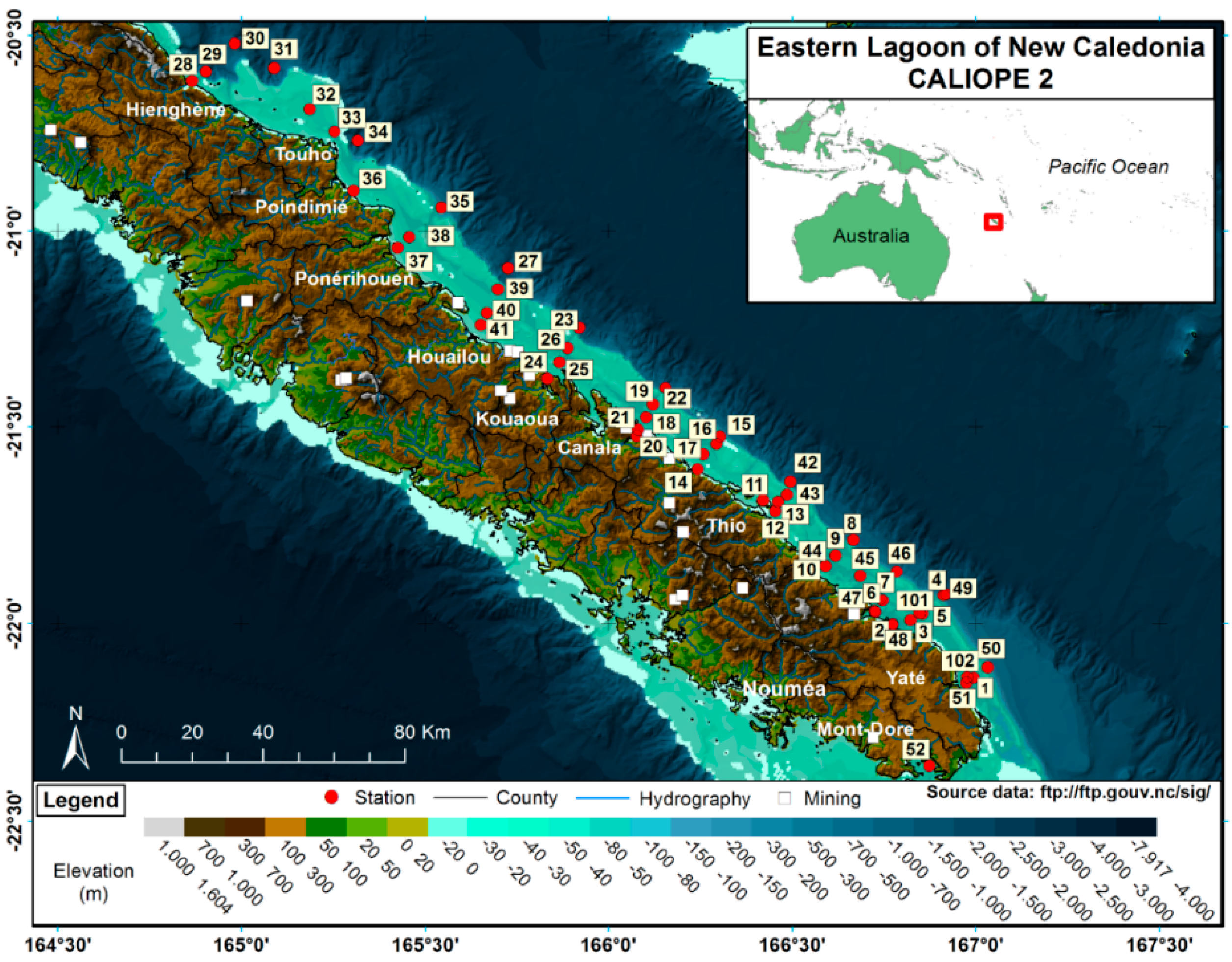
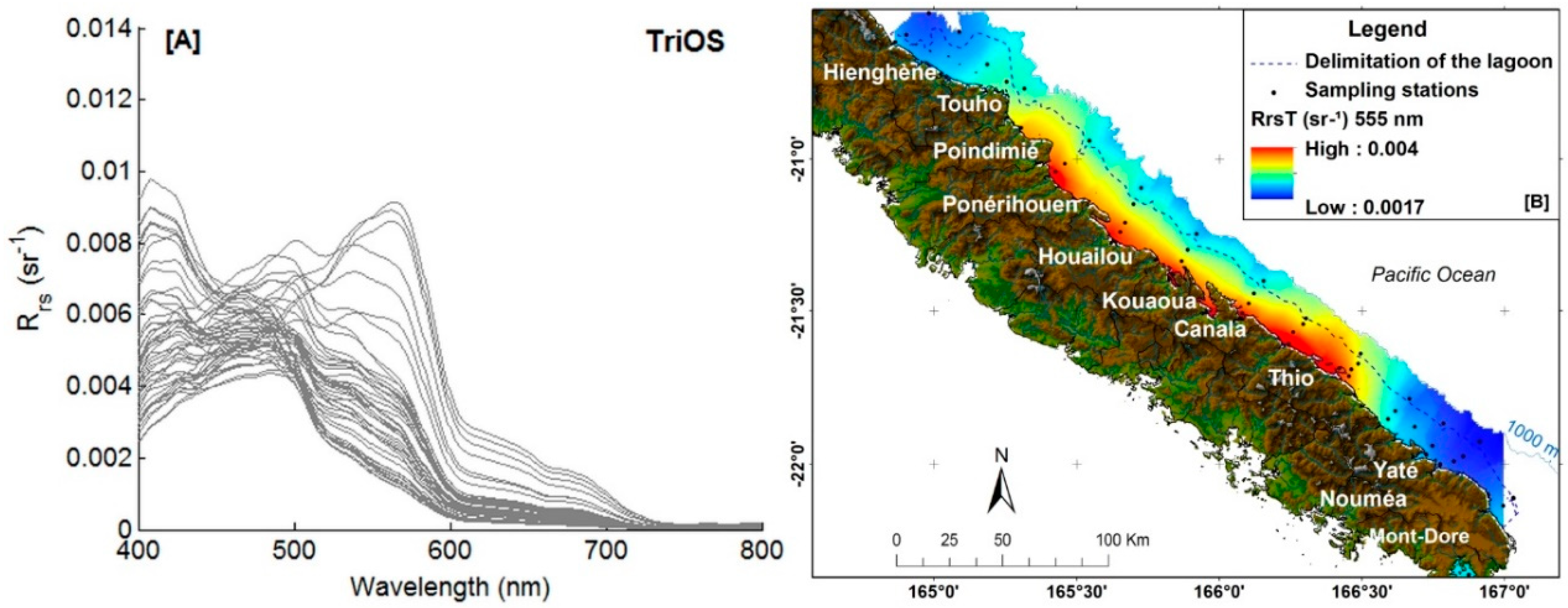
2.1. Study Area

Located in the western South Pacific Ocean, the reef structures and ecosystems of New Caledonia extend between the latitudes of 18°S and 23°S and longitudes of 162°E and 168°E. The reefs permeate the entire island forming lagoons surrounded by a continental shelf with a steep slope. The ELNC has approximately 300 km of extension, located between the villages of Yaté and Hienghène (Figure 1). It is the deepest lagoon in New Caledonia with maximum depths of ~80 m, and is semi-enclosed by a coral reef barrier located between 5 to 25 km from the coastline. The lagoon is connected to the adjacent Pacific Ocean, through strait passages that allow the intrusion of oligotrophic oceanic waters forced by tides, trade winds, and circulation of the external Vauban Current [50]. On the continental side, there are many small and medium size rivers that contribute to the system, as well as several mining sites [10,51]. Compared to the western lagoons, the ELNC is deeper and has more restricted connections to the open ocean, through strait passages [9,10,47]. The austral spring-summer is generally hot and rainy, with more intensive showers extending through January to March, whereas the austral autumn-winter (March to September) is generally dryer and marked by more intensive southeast trade winds [52,53]. The coastal lagoons of New Caledonia are typically dominated by oligo-mesotrophic waters throughout the year (~0.3 mg·m⁻³ of Chla), with strong influence of the adjacent ocean. However, during the rainy season, and especially after intensive rainfall events, that wash out the eroded soil, organic and inorganic sediments, as well as nutrients that enhance phytoplankton growth, are carried into the lagoon increasing the water turbidity and altering the trophic state [9,10,42].

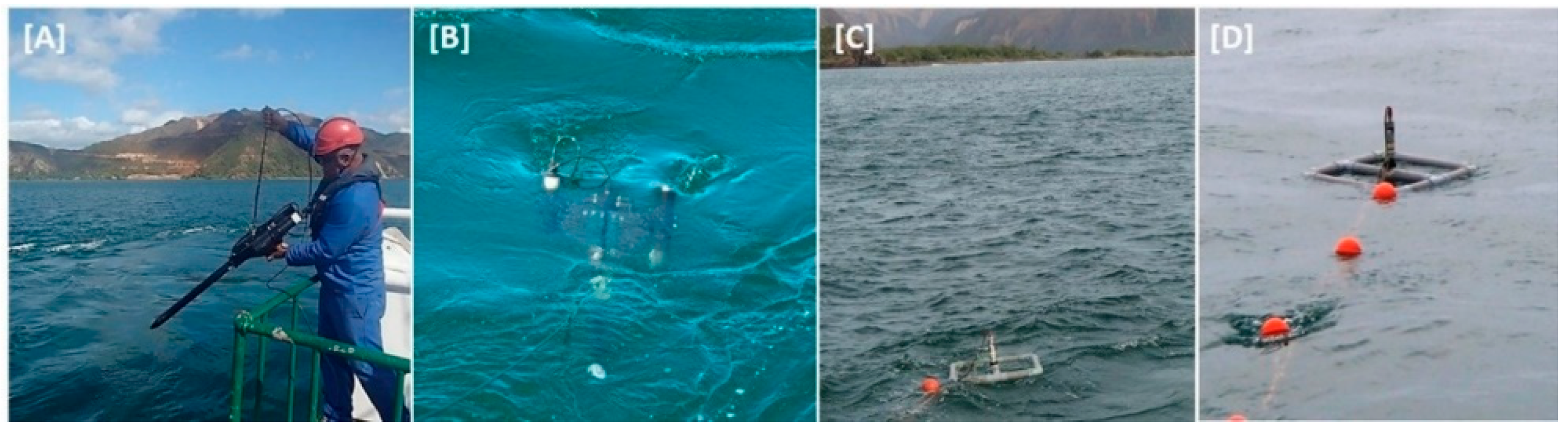
2.2. Oceanographic Campaign

The oceanographic cruise CALIOPE 2, was conducted from 8 to 21 of March 2014. A total of 55 stations were sampled from the south (Yaté) to the north of the lagoon (Hienghène), distributed within 12 transects perpendicular to the coastline, up to the open ocean, across the coral reef barrier (Figure 1). At each station collections were made to determine: (i) meteo-oceanographic conditions, including: wind speed, sea surface temperature, and salinity (with a CTD probe SBE19); (ii) biogeochemical properties, i.e., turbidity and Chla; (iii) bio-optical properties, i.e., phytoplankton, CDOM and NAP light absorption coefficients, and marine b_bp, and (iv) radiometric properties, i.e., downwelling solar irradiance and upwelling radiance.

2.3. Biogeochemical and Bio-Optical Properties

In situ water turbidity was obtained by a ECO FLNTU (Wetlabs Inc., New Caledonia, France) turbidimeter profiler that measures the light scattered at 140 degrees from a 700 nm LED light source, and converts the signal into NTU using calibration coefficients and the Formazin Standard provided by the manufacturer. Surface water turbidity was obtained by averaging the profile measurements within the first 3 m.

The collection and processing of the bio-optical data are the same as described in Dupouy et al., [9,40,41,42]. Vertical profiles of the backscattering coefficient (b_b, m⁻¹) were measured using a Hydroscat-6 (HobiLabs) scatterometer calibrated 1 month before the cruise, with 10 nm bands centred at 442, 488, 510, 550 nm, and 20 nm bands at 620 and 670 nm. Data was processed using the manufacturer calibration files and volume scattering function (β), and corrected for the path length signal loss due to absorption (sigma correction) [54]. The seawater b_b used to obtain the b_bp was determined following Twardowski et al. [17] adjusted for the mean salinity of the lagoon. The surface water b_bp value was determined by averaging the first depths (1–5 m), to avoid noise caused by bubble clouds and in-water perturbations.

For analysis of the light absorption coefficients and Chla, water samples were collected at a sub-surface depth of ~2 m with a rosette Niskin bottle system. Samples for determination of phytoplankton pigments and the particulate absorption coefficient were immediately filtered on board (1–2 L), using 25 mm GFF (0.7 μm nominal pore size). The filters were stored in liquid nitrogen for laboratory analysis. The Chla was determined by two methods: (i) using an adapted fluorometric method after 90% methanol extraction, and subtracting for pheopigments after acidification [9,40,41,42], and (ii) by High Performance Liquid Chromatography (HPLC) [55] (analysed by Crystal Thomas, NASA laboratory). The mean percent difference between the two measurements was lower than 10% indicating good accuracy. We used the HPLC total Chla (TChla) as the reference value and the fluorimetric Chla to determine the standard deviation as an uncertainty metric.

The CDOMl light absorption (a_cdom) from 250–750 nm was measured on board using the UltraPath method (World Precision Instruments Inc.), after filtration of the sample through a 0.2 μm pore sized membrane filter, pre-washed in a 10% HCl solution and rinsed with MilliQ water. The blank reference was prepared to have similar salinity with addition of pre-combusted NaCl. The path length was adjusted from 2 to 0.1 m according to each sample. Salinity and temperature corrections were performed following Röttgers et al. [56].

The particulate absorption coefficient (a_p) was determined using the Quantitative Filter Technique (QFT) adapted from Mitchell [57], following Röttgers et al. [18], with a portable Integrating Cavity Absorption Meter setup (QFT-ICAM). First the total light absorption of the particulate material is measured on the filter sample using the ICAM spectrophotometer to determine a_p. Then the filter is exposed to a solution of 10% NaOCl for ~5 min, to bleach the phytoplankton pigments, and is measured again in the spectrophotometer to determine the light absorption of the non-algal particles (a_nap) [58,59]. The path length amplification factor (β) due to filter multiple scattering was determined for each sample by comparing the particulate absorption measured on the filter with the spectrophotometer, and a_p measured with the Point Source Integrating Cavity Absorption Meter (PSICAM), following Röttgers & Doerffer [59], Röttgers et al. [56] and Röttgers et al. [18]. At last, the phytoplankton absorption coefficient (a_phy) was determined by subtracting a_nap from a_p. Total absorption (a) was obtained by summing a_p+a_cdom with the pure water absorption coefficient (a_w) [60]. The mean percent difference between a_p pseudo triplicates (water filtered from the same cast) were less than 10% within the visible spectrum (400–700 nm).

For the a_p PSICAM measurements, first the cavity is filled with purified water and absorption measurements are taken to obtain a mean reference spectrum between 350 and 720 nm. In the following, the water sample is poured into the cavity and the total absorption is measured. The cavity is washed and filled again with purified water and then filled with filtered water samples (0.2 μm) to determine a_cdom. The particulate absorption is then determined by subtracting a_cdom and the pure water reference absorptions from the total absorption.

Since standard ocean colour algorithms do not differentiate CDOM absorption from a_nap, as they have a similar spectral dependency, for the purpose to evaluate the ocean colour algorithms, we summed these terms, referring to them as a_dg. The spectral slopes (S) of a_cdom (S_cdom), a_nap (S_nap) and a_dg (S_dg) were determined by applying an exponential fit to each spectrum between 350 and 500 nm. For b_bp the spectral slope (S_bbp) was determined using a power law fit for each station within 443–555 nm. The specific phytoplankton absorption coefficient (a_phy*) was determined by normalizing a_phy with Chla.

2.4. Radiometric Measurements

Radiometric data was collected using two types of in-water radiometers: (i) the free-falling Satlantic profiler and (ii) TriOS sensors, attached to a floating structure (Figure 2C,D), for comparison and uncertainty determination. The Satlantic free-falling profiler radiometer (Hyperpro-II) (Figure 2A,B) measures radiance between 350 and 800 nm (3.3 nm bandwidth). With this instrument radiometric data was obtained at 40 stations with in-water profiles of downwelling irradiance (E_d(λ,z)) and upwelling radiance (L_u(λ,z)). Data was pre-processed using the Prosoft software with the instrument calibration files, and some profile editions to eliminate noise (using tilt and velocity thresholds). To make the profiles even smoother, filtering out noise caused by wavy facets and bubble clouds, a second order polynomial fit was also applied to each profile. To extrapolate E_d(λ,z) and L_u(λ,z) to just below surface values (0⁻), the diffuse light attenuation coefficients (K_d(λ) and K_u(λ), respectively) were determined using the intercept of the linear regression fit of the log transformed data (assuming an homogeneous profile). The depth interval used to determine K_d and K_u varied at each station from 5–15 m, depending on the size of the profile and avoiding noisy intervals. After the extrapolation of L_u(λ) and E_d(λ) to 0⁻, they were extrapolated to just above surface (0⁺), i.e., L_w and E_d(0⁺), using air-water transmittance factors [61]. The R_rs determined with the Satlantic free-falling profiler (R_rsS) was finally obtained by the ratio of L_w/E_d(0⁺).

The light penetration depth (Z₉₀), above which approximately 90% of the R_rs signal is originated, can be approximated by 1/K_d(λ) [62]. Hence, Z₉₀ was also determined for each station, within the visible spectral range (400–700 nm), to verify possible influences of bottom reflectance on the above-water R_rs within the stations sampled at the ELNC.

Radiometric data obtained with the TriOS-RAMSES sensors was measured using two hyperspectral radiometers SAM-ARC-Vis: one for the sub-surface (~2 cm) L_u(λ) deployed with an adapted floating system (Figure 2C,D), and another for the above-water downwelling irradiance (E_s(λ)) installed at upper most level of the vessel (deck sensor). These measurements were made at 49 stations (9 more than with the Satlantic profiler). The TriOS instruments measure radiance and irradiance from 320 to 950 nm, with 3.3 nm bandwidth resolution (7 nm bandwidth). To minimize platform shading effects and in-water perturbations which may bias in-water profiling systems winched beside the vessel [15,63], the in-water TriOS sensor was attached to a PVC floating structure connected to a cable with buoys, and deployed to drift away and collect sub-surface L_u data at least 15 m distant from the platform [64]. The sub-surface L_u was extrapolated to surface water leaving radiance (L_w) using air-water transmittance factors [61], and the above-water TriOS R_rs (R_rsT) was obtained with the ratio of L_w/E_s.

For the comparisons between the two approaches, and to further apply the radiometric data to the ocean colour algorithms, the hyperspectral R_rs measurements were used to simulate correspondent bands of the MODIS-Aqua sensor centred at 412, 443, 490, 510 and 555 nm with 10 nm bandwidth. Both the Satlantic and TriOS R_rs data were corrected for variations in solar zenith angle (SZA) to obtain equivalent values for the Sun at zenith, using f/Q factors provided by Morel et al. [65].

A closure experiment was also performed to evaluate the consistency between the radiometric measurements and bio-optical data. The experiment was approached by comparing the measured R_rs with forward modelled R_rs, using the measured absorption (a) and backscattering (b_b) coefficients. The measured R_rs used for these comparisons (as well as for the application of the bio-optical algorithms), were the ones obtained from the TriOS instruments, since there was a higher number of sampled stations (N = 49). The standard deviation of the R_rs obtained by the two in-water approaches, was used as an uncertainty estimate for the in situ radiometry. The modelled R_rs was obtained using approximations of the radiative-transfer equation (RTE), with environmental and bidirectional factors following Morel et al. [65], Gordon et al. [29], and Park and Ruddick [66]. The Gordon et al. [29] approximation uses a quadratic function with two factors i.e., l₁ = 0.0949 and l₂ = 0.0794, that relate the sub-surface remote sensing reflectance (r_rs) to the IOPs i.e., r_rs = l₁ (b_b/(a + b_b)) + l₁ (b_b/(a + b_b))². This approximation is simple and very practical for ocean colour applications, being used in common inversion algorithms e.g., GSM, QAA, GIOP. The Morel et al. [65] approximation uses a ratio of two factors (f/Q), that are spectrally dependent, and vary with the Chla, to account for variations in the scattering phase function, when relating R_rs to the IOPs i.e., R_rs = ℜ f/Q (b_b/a) (ℜ is the air-water transmittance factor). This approximation is more elaborated, but appropriate solely for open ocean or coastal waters where phytoplankton and covarying detritus dominates the light absorption and scattering, as the scattering phase function is dependent solely on Chla, and b_b should be much smaller than a. Since the ELNC is, however, also subjected to river outflows that may potentially carry in suspended sediments, we also tested the Park and Ruddick [66] approach. The approximation in this case, uses a fourth order polynomial function that relates R_rs to the IOPs, with four environmental and bidirectional factors (g_i(λ), i = 1–4) that vary with the ratio of b_bp:b_b (as well as wind speed–considering nadir viewing geometry and Sun at Zenith) to account for variations in the volume scattering phase function with the bulk particle assemblage. The standard deviation between the modelled R_rs (R_rs RTE) obtained by the 3 approximations was used as an uncertainty measure. Other sources due to propagation of IOP uncertainties and inelastic scattering (i.e., Raman scattering) were not quantified, but only discussed for simplicity.

The comparisons between the R_rs measurements, as well as with the forward model retrievals, were made using standard metrics of radiometry inter-comparisons, i.e., the coefficient of determination (R²), the root mean square error (RMSE), the relative mean percent difference (RPD) (in absolute values) (RPD = Σ[|x₁ − x₂|/x₂]/N) × 100), where x₂ is the reference), and the unbiased percentage difference (UPD) (UPD = Σ[(x₁ − x₂)/((x₁ + x₂)/2)]/N) × 100)) [14,15]. The UPD presupposes that all methods are somewhat biased and indicates there is an over (positive) or under (negative) estimation of a method in respect to the other. The RPD was used to quantify the total error relative to a least biased “reference”.

2.5. Bio-Optical Algorithms

Ocean colour bio-optical algorithms were tested using the in situ measured R_rs (from the TriOS instrument). For Chla determinations the algorithms that were tested for the ELNC were: the empirical OC3M and OC4 [22], and the semi-analytical GSM01 [27,28] and the GIOP [32]. To estimate the absorption and backscattering coefficients we applied the GSM01, GIOP, QAA [30] and the LMI, in this case regionally tuned for New Caledonia coastal lagoons [36,37].

Surface water turbidity algorithms were also applied to the ELNC with in situ data obtained during the CALIOPE 2 campaign, testing 3 approaches: (i) the regional algorithm proposed by Ouillon et al. [38]; (ii) the global algorithm for tropical coastal waters also proposed by Ouillon et al. [38] and (iii) the single global algorithm for all water types proposed by Dogliotti et al. [39]. Although turbidity measurements use the same chemical standard i.e., Formazin, they are specified in different units according to methods and instruments. As this may be a source of discrepancy in the application of the algorithms, we specify the corresponding units used in each approach. Turbidity measured by Ouillon et al. [38] was obtained using a SeaPoint optical turbidimeter that measures the scattered light at 880 nm, in a broad viewing angle of 15–150 degrees, and the units are given in Formazin Turbidity Units (FTU). Turbidity measured by Dogliotti et al. [39] were obtained using portable HACH 2100P and 2100QIS turbidimeters, which measure the side-scattered light at 860 nm, at 90 degrees, and the units are given in Formazin Nephelometric Units (FNU). As previously described, we used a ECO FLNTU (Wetlabs Inc., New Caledonia, France) turbidimeter that measures the scattered light at 700 nm at 140 degrees, and the units are specified in Nephelometric Turbidity Units (NTU).

All the retrievals were compared to the in situ measurements using statistical metrics of linear regression: the slope, R² and RMSE, and the relative mean percent difference (RPD).

3. Results and Discussion

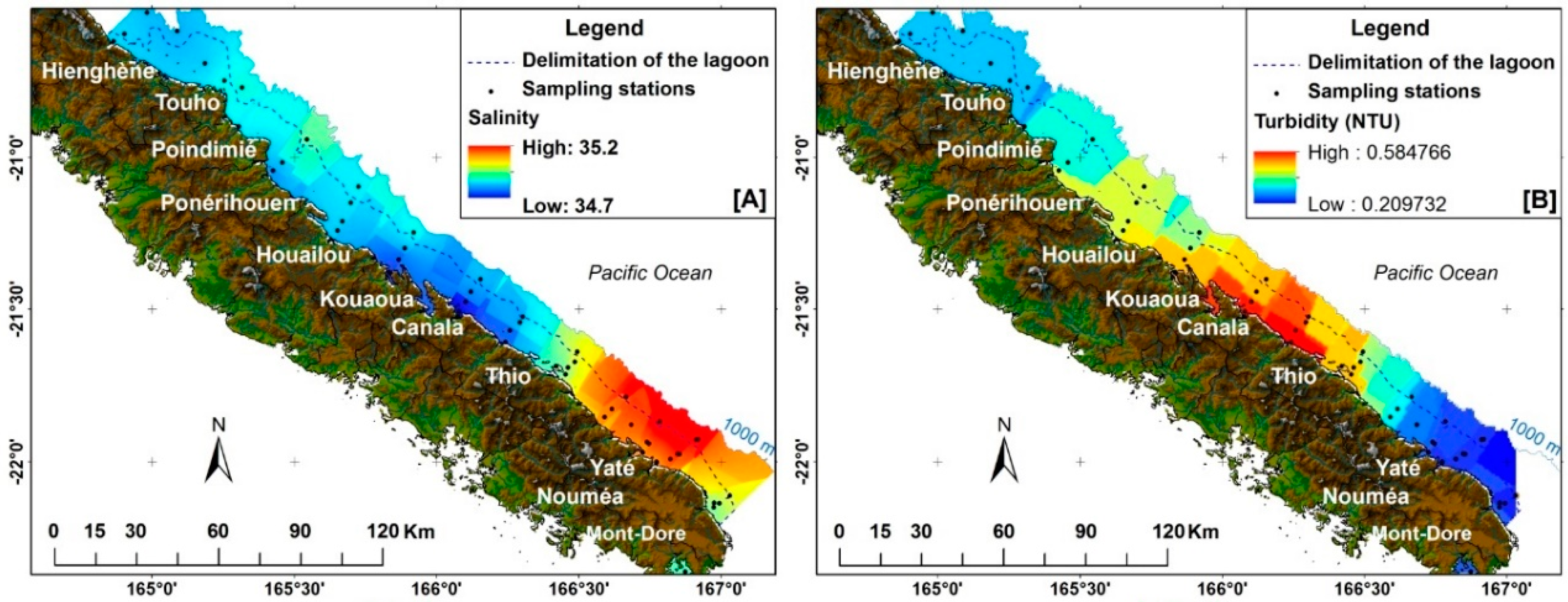
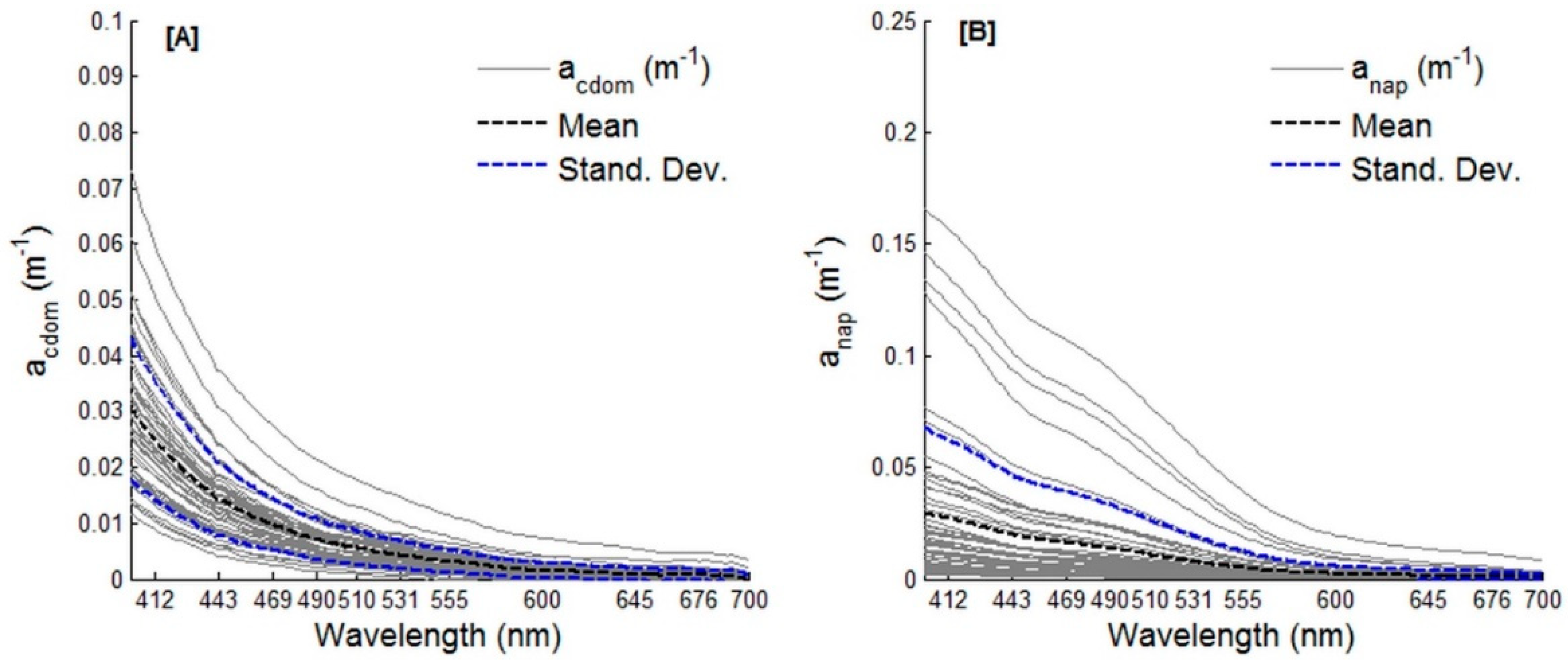
3.1. Environmental and Bio-Optical Characterization

During the CALIOPE 2 campaign, in late summer 2014, although cloud coverage was high, the rainy season was late, and contribution of river runoff was lower than during CALIOPE 3, but still somewhat higher than during CALIOPE 1 in the dry winter season [9,10]. The wind intensity during CALIOPE 2 was also much higher (up to 16 m·s⁻¹) than CALIOPE 1 [9], contributing to the higher water turbidity with a well-mixed water column and bottom re-suspension in shallow areas near the coast (as noticed in the vertical turbidity profiles–not shown). The biophysical parameters of the surface waters had a relatively small range of variability, with water temperature varying from 26.2–28.1 °C, salinity between 35.2–34.7 and turbidity between 0.12–1.09 NTU. The southern tip of the lagoon was characterized by colder, more saline and less turbid waters (Figure 3), suggesting a greater influence of oceanic oligotrophic waters due to local circulation [9,10]. Coastal upwelling, which occurs especially during spring and summer, in southwest New Caledonia [44,67], can also contribute to bring colder and more saline waters into the southern lagoons [44,47]. The inner coastal stations, especially in the central lagoon, between the villages of Houailou and Thio, were the ones with lowest salinity and highest turbidity (Figure 3). Besides of river runoff, this region has 11 mining sites that contribute to increasing surface water turbidity and accumulating sediments within the lagoon, especially after intensive rainy events that wash out the eroded soil [9,42].

The surface Chla varied from 0.136 ± 0.001 to 0.725 ± 0.112 mg·m⁻³, with an average of 0.370 ± 0.163 mg·m⁻³, presenting characteristics of oligo-mesotrophic waters. Higher Chla values were obtained at the coastal stations between the villages of Canala and Thio, which had lower salinity (~34.8) and higher turbidity (~1 NTU), indicating that a greater influence of river runoff enhances phytoplankton growth in this central sector of the lagoon. Bottom resuspension forced by strong and persistent winds (>7 m·s⁻¹) also favours the phytoplankton growth at these shallower stations (11–17 m) [9]. Hence, during CALIOPE 2, the surface Chla was higher than the observed during CALIOPE 1 in the dry and calm winter season (October 2011) (mean ~0.21 mg·m⁻³ and maximum 0.60 mg·m⁻³) [9], suggesting a higher contribution of river runoff and resuspension processes, even though the rainy season was late. In the following summer campaign, CALIOPE 3 (March 2016), which captured a greater influence of continental drainage and river runoff, the surface Chla had a close average (0.37 ± 0.7 mg·m⁻³), but a higher range of variability, i.e., 0.02–3.51 mg·m⁻³, compared to CALIOPE 2 [10].

The a_phy(443) varied from 0.007 ± 0.0003 to 0.037 ± 0.002 m⁻¹, with an average of 0.018 ± 0.007 m⁻¹ (Figure 4A), and a positive co-variation with Chla (R² = 0.86). Variability in the relation between a_phy(443) and Chla can be due to non-linear packaging effects associated to the phytoplankton community structure and photo-adaptation processes [27,28,31]. The specific absorption coefficient a_phy*(443) (normalized by Chla) varied from 0.032 to 0.067 m²·mgChla⁻¹, with an average of 0.049 ± 0.008 m²·mgChla⁻¹ (Figure 4A), typical of populations mostly dominated by nanoplankton cells [28], as found in New Caledonia coastal lagoons [10,43,44]. The lowest a_phy*(443) values (~0.032 m²·mgChla⁻¹) were obtained at the coastal stations (e.g., stations 14, 16, 20 and 24), which had higher TChla (>0.6 mg·m³) and higher proportions of Fucoxanthin, suggesting the dominance of diatoms (>40%) (following the relation proposed by Uitz et al. [68] and updated by Hirata et al. [69] with the diagnostic pigments determined by HPLC). The highest a_phy*(443) values (~0.067 m²·mgChla⁻¹) were obtained at the stations across the coral reef barrier, at the shelf slope (>300 m deep) (e.g., stations 22 and 23), with lower TChla (<0.2 mg·m³) and higher proportions of diagnostic pigments of picoplankton groups (Zeaxanthin, Chlb and DVChla), suggesting the dominance of these groups (>60%) [68,69]. The negative relation between a_phy*(443) and Chla associated to the dominance of different phytoplankton groups (and size classes) has been well reported in other works [23,34,70].

There was however a highly dispersive relation between a_phy*(443) and Chla (R² = 0.15), and with a_phy*(443) values mostly below those expected for the correspondent Chla, according to the global relation obtained by Bricaud et al. [23] (Figure 4B). This denotes the high complexity of the ELNC waters with “local” variations of the specific optical properties (“local” meaning both in respect to the geographic region and season). A source of variability in the a_phy*(443) could be also due to photo-acclimation processes [24,70]. Even with relatively low phytoplankton biomass (mean, 0.37 mg·m⁻³ of Chla), these cells need to compete with NAP and CDOM (which have extra sources in the ELNC result of mining activities), to absorb the underwater light. This competition for light, at overlapping absorbing peaks, poses an additional condition for photo-acclimation processes, in which the phytoplankton cells need to increase its bulk absorbing capacity, increasing the intracellular Chla, and consequently increasing pigment shading effects, which diminishes a_phy*. Hence the phytoplankton cells of the ELNC may have lower a_phy* values due to the “extra” light competition with CDOM and NAP absorption.

Part of the deviation from the “global” relation of a_phy*(443) and Chla could however, also be due to methodological issues. Stramski et al. [71] shows how using different methods and path length amplification factors (beta correction) can cause over than 30% differences for the a_p measurements. Particularly, they showed how the transmittance QFT method (as used to determine the a_phy(443) and Chla relation by Bricaud et al. [24]) tends to overestimate a_phy(443) in respect to measurements obtained inside an integrating sphere (as used herein following Röttgers et al. [18]). This a problem to be considered when integrating data sets obtained from different cruises and analysed by different methods [71].

The a_cdom(443) had a mean value of 0.014 ± 0.005 m⁻¹ (Figure 5A), and was more correlated to turbidity (R² = 0.60) than Chla (R² = 0.31), indicating the influence of allochthonous sources in the lagoon. Martias et al. [10] made a thorough description of the different sources of CDOM in the ELNC, citing river runoff, coastal erosion (linked to mining activity), bottom re-suspension, as well as releases from the coral reef benthic community, besides of the autochthonous sources linked to the phytoplankton. The highest a_cdom(443) values were observed at the coastal stations of the central sector (maximum 0.037 m⁻¹) near the main rivers, and the lowest at the southern tip (minimum 0.004 m⁻¹), with greater influence of oceanic waters [9]. Regarding the a_cdom(λ) spectral slope (S_cdom), the observed values were also similar to those reported at the other CALIOPE campaigns in the ELNC (mean, 0.017 ± 0.002 nm⁻¹), with the lowest values near the main rivers (minimum 0.014 nm⁻¹) and highest (maximum 0.023 nm⁻¹) at the southern sector and outside the reef barrier, where water transparency favours photo-oxidation processes [10,26].

The a_nap(443) was on average higher than a_cdom(443), with a mean of 0.02 ± 0.018 m⁻¹ (Figure 5B). The highest values (~0.10 m⁻¹) were observed at the coastal stations near Kouaoua and Houailou, and the lowest at the southern tip of the lagoon (~0.001 m⁻¹). The distribution of a_nap was well explained by turbidity (R² = 0.92) and only weakly explained by Chla (R² = 0.4), indicating the contribution of allochthonous particles in the system. A positive linear correlation (R² = 0.79) was obtained between a_nap(443) and a_cdom(443), suggesting that both components have some similar sources in the ELNC, including river runoff, erosion from mining sites, the coral reef, which can also be a source of NAP [10,72], besides autochthonous sources. The mean a_nap spectral slope (S_nap) was ~0.010 ± 0.002 nm⁻¹, which is close to the average reported by Bricaud et al. [73] for stations collected in the surface layer of the southeast Pacific Ocean (0.009 ± 0.018 nm⁻¹), and somewhat lower than values obtained by Babin et al. [74] in coastal waters around Europe (mean 0.0123 nm⁻¹, varying from 0.0116–0.013 nm⁻¹). The highest S_nap values (~0.013 nm⁻¹) were associated with the clearest oceanic oligotrophic waters, with lower a_nap(443) values. The lowest S_nap values (~0.006 nm⁻¹) were obtained at the turbid coastal stations near the mining sites, with higher a_nap(443). An inverse relation between S_nap and a_nap was also obtained by Bricaud et al. [73], although with a high dispersion indicating a complex relation between the bulk particle pool and the coloured fraction. Although within a low range of variability Babin et al. [74] discussed that lower S_nap values in coastal waters could be associated to a greater contribution of mineral particles. Summing the CDOM and NAP absorption coefficients, the mean spectral slope was 0.014 ± 0.002 nm⁻¹, varying from 0.009 to 0.020 nm⁻¹.

It should be noted that there were spectral features in a_nap(λ) deviated from a typical exponential curve, with a “shoulder”-like feature between 460–580 nm (Figure 5B). This feature could be due to iron absorption, adsorbed to the suspended sediments [74,75], as New Caledonia has iron-rich laterite soil [51] that is eroded and lixiviated into the lagoon especially near the mining sites [42].

The total light absorption by constituents other than pure seawater (i.e., a_phy + a_nap + a_cdom) at 443 nm was mainly dominated by NAP at the shallowest stations (11–22 m) located near the coastline (maximum, 69%). At the deeper stations towards the reef barrier (>40 m depth) and across to the open ocean (>75 m), however, the non-water absorption was dominated either by phytoplankton (maximum, 64%) or CDOM (maximum, 48%) (Figure 6). The variability in the proportions of the absorption by each constituent within the ELNC is rather high for an oligo-mesotrophic tropical lagoon, with relatively clear waters (<1.09 NTU). Even with a strong influence of the oligotrophic waters of the adjacent ocean, and a minor influence of river runoff due to the late rainy season, the ELNC still had several different sources that affected the water quality and imprinted a complex mixture of optically active constituents, during CALIOPE 2. This mixture poses higher challenges for bio-optical and biogeochemical remote sensing retrievals, especially for the constituents with the least optical influence.

Regarding the marine b_bp at 443 nm, the mean value obtained for the ELNC at CALIOPE 2 was 0.0036 m⁻¹, with a high standard deviation of ±0.004 m⁻¹ (Figure 7A). The highest b_bp(443) values (maximum 0.018 m⁻¹) were obtained at stations located near mining sites between Thio and Touho, in the central ELNC, as for the CALIOPE 1 campaign [9]. Higher b_bp(443) values (~0.0058 m⁻¹) were also observed at the northern sector of the lagoon at CALIOPE 2, probably favoured by re-suspension processes in the shallowest areas. For both campaigns, the southern sector had the clearest waters with the lowest b_bp(443) (~0.004 m⁻¹), resembling clearer waters of the lagoons located in southwest New Caledonia [40,41,42], with greater influence of oceanic oligotrophic waters. The mean b_bp spectral slope (S_bbp) was 0.07 ± 0.1 nm⁻¹, which is small compared to the values typically obtained in open ocean waters (between 1 and ~3) [25] and likely associated with dominance of larger organic and inorganic particles.

The b_bp(555) had a weak positive relationship with Chla (R² = 0.34) and a_phy(443) (R² = 0.42), but a strong relationship with a_nap(443) (R² = 0.84) (Figure 7B). This suggests that the non-algal particles present in relatively high proportions within the lagoon (especially at the central coastal stations) dominated the particulate light backscattering coefficient. The a_cdom(443) also had an indirect but strong positive relation with b_bp(555) (R² = 0.76), reinforcing that NAP and CDOM had some similar sources within the lagoon, which also influenced b_bp(555) e.g., river runoff, bottom re-suspension, mining activity, and the coral reef ecosystem, besides of the autochthonous sources.

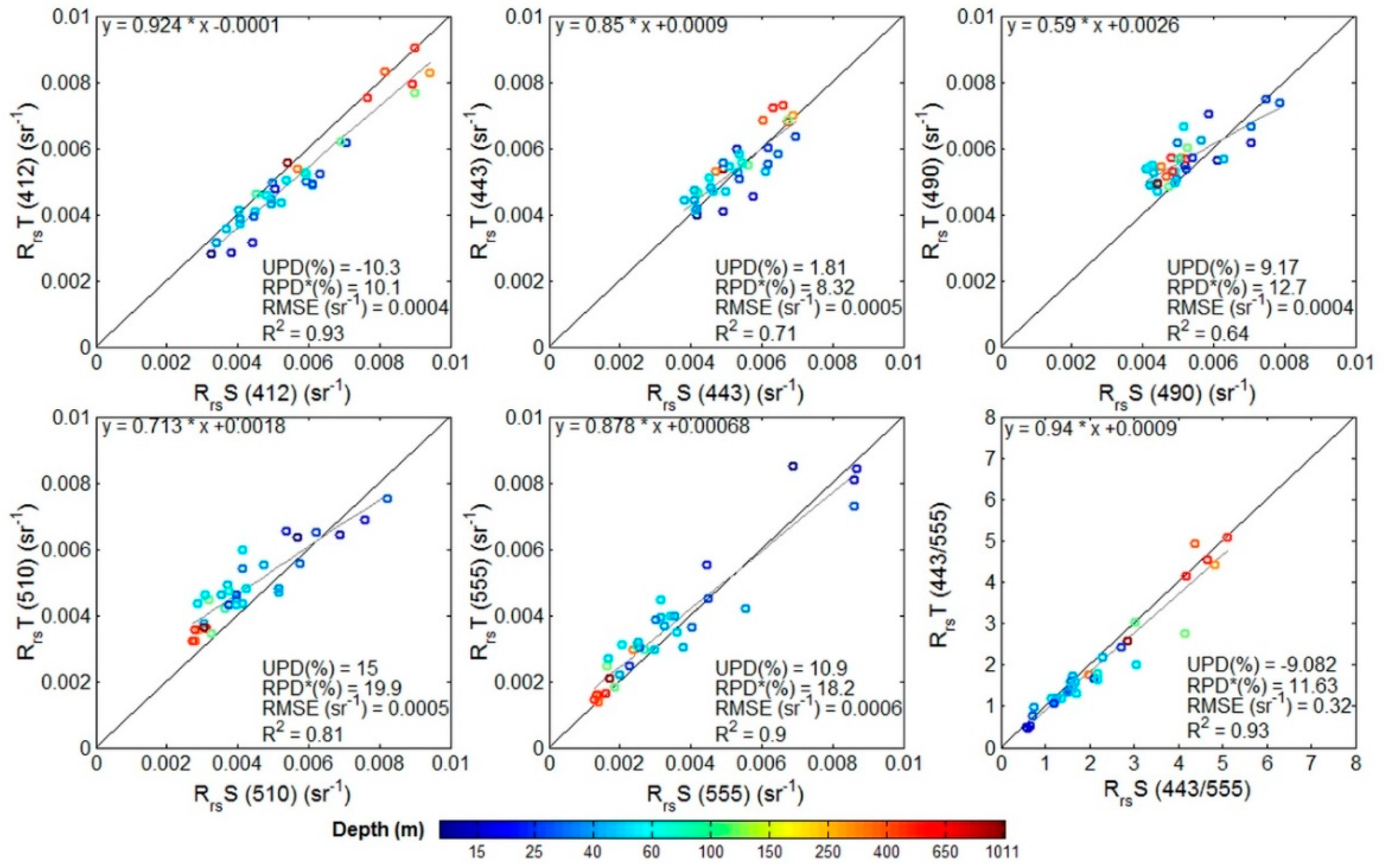
3.2. In Situ Radiometry

Of the 54 stations sampled during the CALIOPE 2 campaign, approximately 50% had cloud cover higher than 5/8 and 14 stations were sampled with high SZA (≥60°) (early in the morning and late afternoon). Strong southwest winds were predominant during the data collection (average speed, 8.5 m·s⁻¹ and maximum 16 m·s⁻¹), indicating rough conditions for in situ radiometric measurements.

The R_rs spectra characteristic of clear waters with higher values at shorter wavelengths (<490 nm), were obtained at the deepest stations across the coral reef barrier, and at the southern and northern tips of the lagoon, where oceanic waters have greater intrusions. Near the main rivers, and especially close to the mining sites (between Thio and Ponérihouen), the R_rs spectra were characteristic of water types dominated by biogenic constituents, that absorb more light in the blue wavelengths, resulting in lower R_rs (<490 nm), and mineral particles that are highly scattering and contribute to higher R_rs at longer wavelengths (>500 nm) (Figure 8).

According to the Z₉₀ test, only one station had potential influence of bottom reflectance on the above water R_rs, located at the northern tip of the lagoon, where clear oligotrophic waters were dominant even at the shallowest station near the coast (station 28). At this station the local depth was 11 m, whereas the first optical depth (~1/K_d) reached a maximum of 19 m at 490 nm. Since this was a unique case for the stations sampled at CALIOPE 2, we decided to remove this station from our analysis for simplicity, and not deal (at this point) with more complex bottom effect processing for ocean colour retrievals (as done by Murakami and Dupouy [37]). The other more coastal stations were located near rivers and mining sites, which had more scattering and absorbing waters, and the first optical depth was always somewhat shallower than the bottom depth (e.g., 5 m for 1/K_d(490) at station 14 with 11 m of bottom depth). The stations with deepest light penetration (~29 m for the first optical depth at 490 nm) were located outside of the lagoon at the shelf slope (>500 m).

3.2.1. Radiometric Comparisons

The R_rsT (TriOS) had a reasonably good agreement with R_rsS (Satlantic), with an absolute percent difference between 8 to 20% at 412–555 nm, and 12% RPD for the R_rs(443:555) ratio (Figure 9). This is within the expected uncertainty for in situ radiometric measurements, which can be somewhat higher than 10% especially under adverse environmental conditions i.e., partly cloudy skies, intensive winds, and within a high range of optical water types [14,15].

The TriOS approach, with the PVC floating structure, yielded lower R_rs values compared with those of the free-falling profiler (Satlantic) especially at the blue bands (412–443 nm) (−10 to 1.8 UPD) at the more coastal and shallow stations (<25 m) (Figure 9). The negative R_rs bias could be explained by light attenuation at the very surface (from 0 to 2 cm) [64] and self-shading effects [76], that are both more problematic for the shorter bands at highly absorbing waters. The R_rs(443) bias was in fact correlated to surface water turbidity with a correlation coefficient r_s, 0.53. The floating PVC structure allowed the TriOS sensor to obtain L_u measurements up to 15 m away from the vessel, avoiding even greater shading effects from the platform [15,63]. Nonetheless, the PVC structure, as well as the instrument itself, can still cause some potential shading.

The R_rsT at the green bands (510–555 nm), on the other hand, had more positive biases (15 to 11 UPD), compared to R_rsS, especially at the deeper stations (>40 m), in the outer reaches of the lagoon (Figure 9). These positive biases were somewhat positively correlated to wind speed (r_s, 0.31), and negatively correlated to water turbidity (r_s, −0.35). The overestimation of R_rs(555) at clearer waters, under intensive winds, could be explained by sub-surface bubble cloud effects. Bubble clouds generated by breaking waves under rough sea conditions (wind speed >7.5 m·s⁻¹), can increase R_rs to more than 10%, especially at yellow-green bands, in clear waters [77]. Since the TriOS in-water sensor sampled L_u measurements at the very surface (~2 cm), whereas the Satlantic profiler sampled at depths from 2–15 m, the TriOS approach was likely much more influenced by sub-surface bubble clouds. As most of the stations of the CALIOPE 2 campaign were sampled under strong winds (>8.5 m·s⁻¹), bubble cloud was a potential source of uncertainty for the in-water radiometric measurements. Another source of positive biases that could be associated to the TriOS approach is the potential additive signal of light reflection from the PVC structure on the in-water L_u(λ).

Both the negative R_rs(443) biases (at the coastal stations), and the positive R_rs(555) biases (at the deeper stations), contributed for the overall negative biases of the R_rsT(443/555) ratio (−9% UPD). The impact of these spectrally uncorrelated biases on ocean colour retrievals, if applied a bio-optical algorithm, would be to overestimate the IOPs (and Chla), especially at the deeper stations with clearest waters, where the biases were larger (Figure 9).

Some other sources of uncertainty of the TriOS approach could be related to mismatches of the illumination condition over the in-water and deck sensors under a fast-changing sky, i.e., partially cloudy. This source, however, should add noise to the dispersion rather than characterize a “systematic” bias. Other sources of uncertainty are also related to the Satlantic free-falling profiler approach, including the use of deeper L_u and E_d measurements, which assumes a homogeneous water column with a constant diffuse attenuation coefficient [78]. Deeper L_u and E_d measurements with lower signal are also more subject to noise and difficult to extrapolate accurately to the surface. Furthermore, the roughened sea surface causes focus and defocusing effects by the wavy facets, which introduces noise to the in-water E_d measurements [79]. All these sources likely contributed to the noisy dispersion in the R_rs comparisons.

Even with all these sources of uncertainty, under mostly adverse environmental conditions, the blue to green R_rs bands and ratio matched reasonably well for the in-water approaches (<20% RPD). The consistency of both methods revealed a good potential of the TriOS adapted approach (with the floating PVC structure) to obtain accurate in situ R_rs. Previous works have shown systematic underestimation of the R_rs derived from TriOS (10 to more than 30%) when winched beside a vessel, in respect to free-falling radiometers, due to strong shading effects from the platform [14,63]. Hence, the adapted TriOS in-water acquisition method appears more suitable, as the radiometer is launched away from the platform avoiding external perturbations on the measurements.

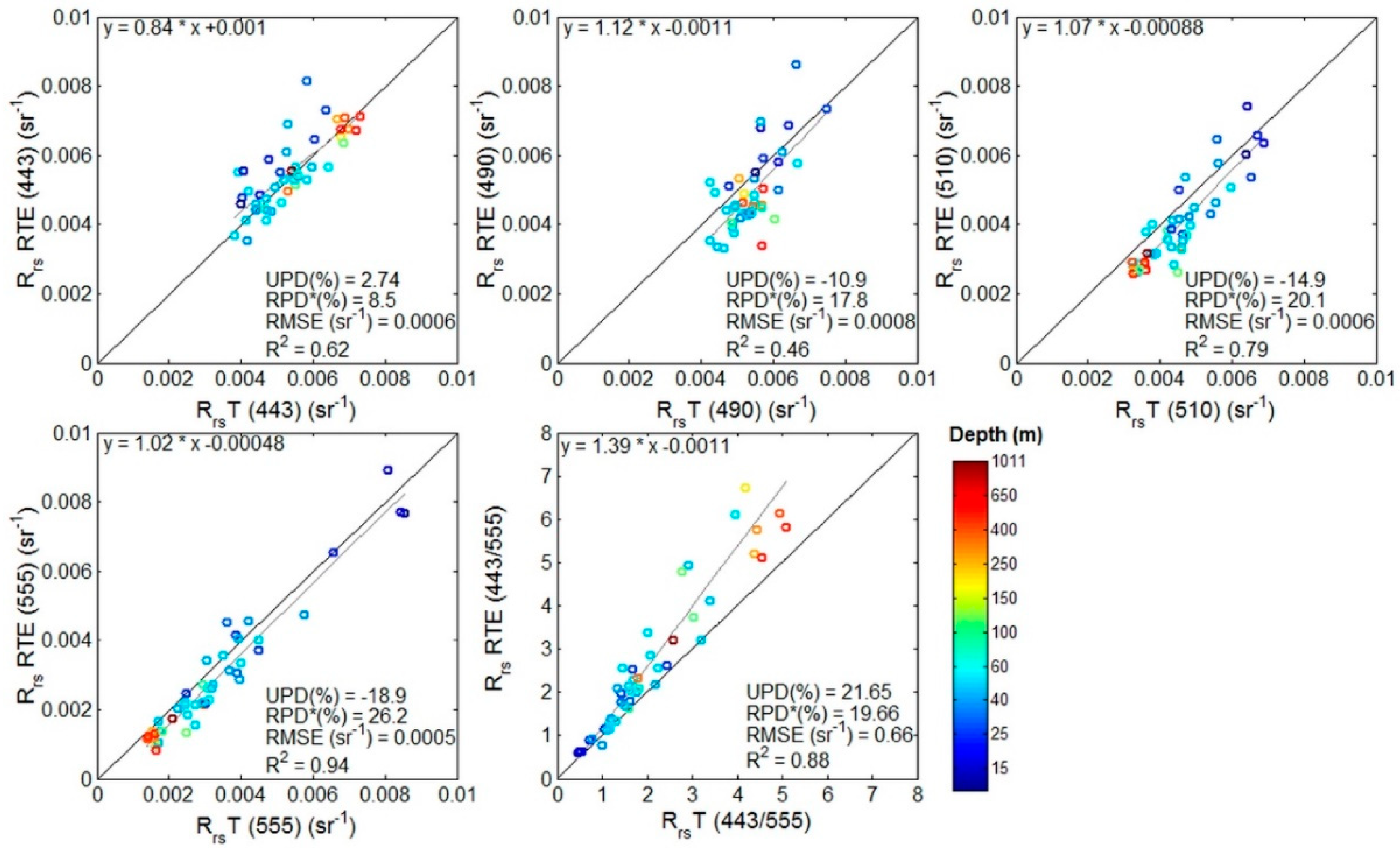
3.2.2. Closure Experiment

Since a greater number of stations were collected with the TriOS approach (N = 48), we show only the results of the closure analysis using the R_rsT. The forward modelled R_rs (RTE), had a mean percent difference of 9 to 26% for the 443–555 nm bands and 20% for the R_rs(443/555) ratio, compared to the measured R_rsT (Figure 10). Closure was not completely obtained even considering the effects of multiple scattering and variations in the β on the bidirectional factor of the modelled R_rs. Closure is always a challenge as there are uncertainties in both the measured and modelled R_rs, and differences over than 30% RPD could be expected across different water types and under adverse environmental [80,81,82,83]. Hence, the absolute differences below 20% point out a reasonably good consistency between the measured IOPs and RTE approximation with the measured R_rs.

The R_rs RTE at 443 nm matched well the measurements, with both positive and negative biases (−1% UPD), whereas the R_rs RTE at the longer bands (490–555 nm) had an overall negative bias with −11 to −19% UPD, leading to a positive bias for the R_rs(443/555) ratio (22% UPD) (Figure 10). Some of these biases could be explained by the R_rsT overestimation at the green bands, due to bubble cloud effects and structure in-water reflection. Comparing the R_rs RTE with R_rsS the biases were somewhat lower, varying from 3 to −6% UPD for the 443–555 nm bands, and 9% UPD for the R_rs(443/555) ratio. This confirms the previous discussion, regarding the underestimation of the R_rs blue:green ratio by R_rsT, under influence of bubble clouds (and structure reflection) especially in clearer waters.

Regarding the modelled R_rs, the sources of uncertainties are related to the approximation of the forward model, the environmental and bidirectional factors used and the measured IOPs. The differences between the environmental and bidirectional factors proposed by other works, i.e., obtained from Morel et al. [65] and Gordon et al. [29], were small (<5%). None of these factors, however consider variations in visibility and cloud cover, as this variability is more difficult to quantify for closure experiments, although it may cause significant differences between the modelled and measured R_rs [63]. Raman scattering is also neglected in these approximations and may account for 4–10% of the measured R_rs > 490 nm, in waters with Chla 0.1–0.5 mg·m⁻³ [83]. Hence, this source may also explain some of the negative biases observed for the modelled R_rs > 490 nm, especially at the clearest waters. Uncertainties in the measured IOPs can also cause differences in these comparisons. The QFT-ICAM method with sample-specific beta factors (measured by PSICAM), should significantly reduce the a_p biases to less than 1% [59]. However, challenges in the sample collection and manipulation may account for 10% differences between triplicates. CDOM absorption measurements are also challenging especially in clear waters, which require the use of a long path length (2 m) using the UltraPath instrument. The long path length increases the signal, but also the probability of interference of small particles and colloids that may remain after the filtration [56], and differences in triplicates are also in order of 10%. Although the water column was well-mixed during the CALIOPE 2 campaign, vertical stratification may also introduce some mismatches between the RTE approximations, which consider homogeneous profiles and use IOPs sampled at a fixed surface depth (2 m) (with exception for b_bp) and the measured R_rs, representative of the integrated first optical depth.

All these sources of uncertainty contributed for the dispersion in the comparisons, and biases between the modelled and measured R_rs. For the coastal stations, the spectral biases were, however, more correlated, and reduced when applying the blue:green R_rs ratio (Figure 10). Whereas, the deepest stations with the clearest waters, had more uncorrelated spectral biases which impacted more the R_rs(443:555) comparison, probably mainly associated to the effects of bubble clouds and Raman scattering. Hence, these sources should also introduce some biases in the performance of the bio-optical algorithms, likely with overestimation of the retrieved Chla and IOPs.

3.3. Bio-Optical Algorithm Evaluation

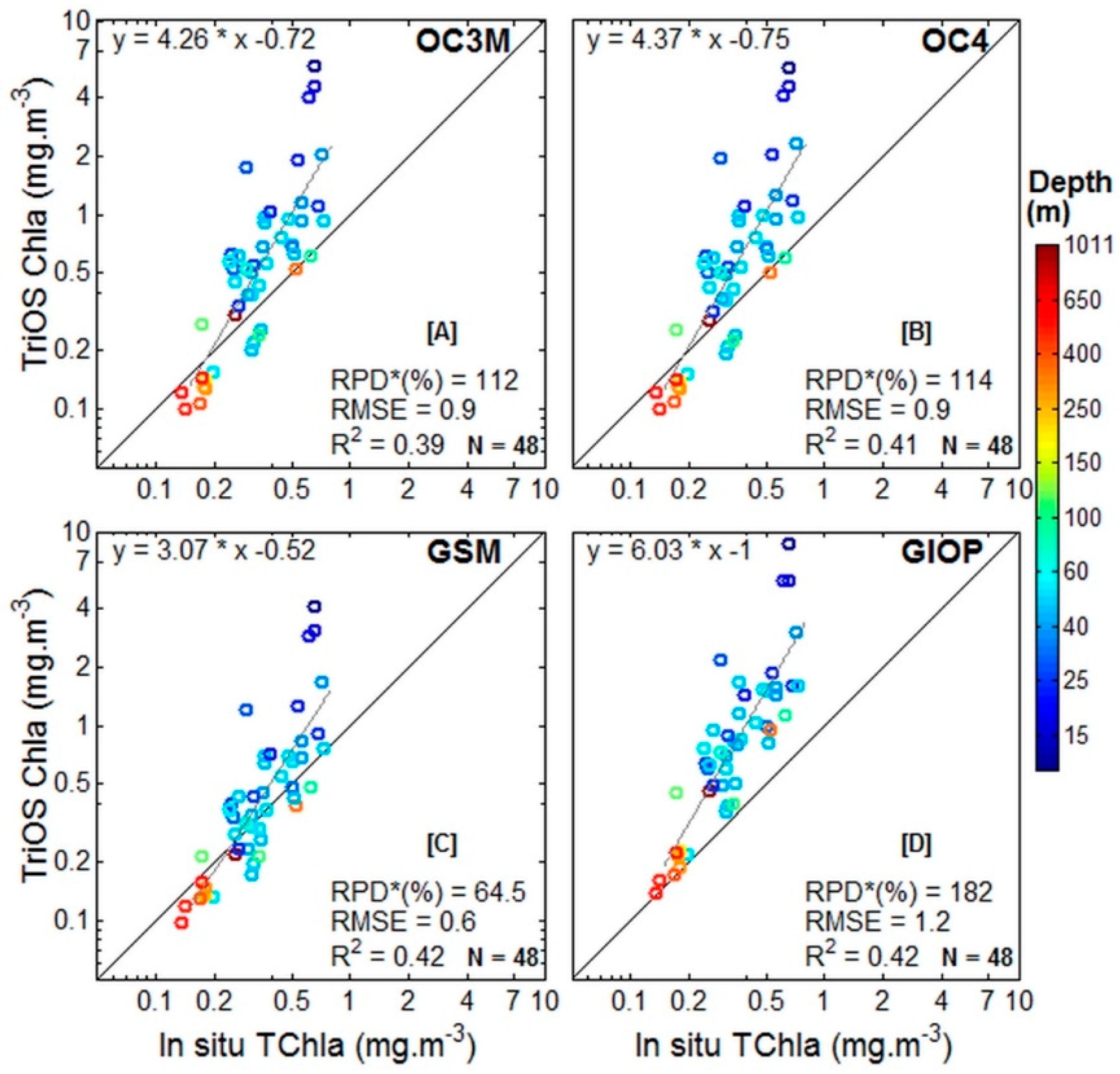
3.3.1. Chlorophyll a Concentration

The empirical and semi-analytical ocean colour algorithms showed similar performance for the Chla retrievals at the ELNC during CALIOPE 2 (with R_rsT), i.e., a positive slope (3–6) ~0.40 R², and a tendency of underestimation at the deeper stations and overestimation at the coastal stations (Figure 11). Taking out the stations with highest surface water turbidity (~1 NTU) and contributions of a_dg to the total non-water absorption at 443 nm (>80%) (Stations 14, 20, 24 and 37), the overall performance for all the algorithms increased significantly, with RPD diminishing from 64 to 35% for GSM01 (0.64 R²), 182 to 122% RPD for GIOP (0.70 R²), and 112 to 68% RPD for OC3M and OC4 (R² = 0.54).

Overestimation of the Chla at turbid coastal waters is expected, especially for the empirical algorithms [12]. The surface water turbidity of the ELNC waters during the CALIOPE 2 campaign was not that high (<1.09 NTU), but as shown in the previous section of bio-optical characterization, there was a complex mixture of the IOPs, with an important contribution of NAP and CDOM to the total non-water light absorption at 443 nm (maximum, 85%). As the GSM01 semi-analytical approach separates the a_dg and a_phy contributions from the total absorption in the inversion scheme, it showed a better performance for the Chla retrieval at the coastal stations compared with the empirical algorithms. There were, however, still some high positive biases at the most turbid stations for the semi-analytical approaches (GSM and GIOP), due to the higher challenges to separate the a_phy and a_dg terms at these stations in the inversion scheme (Figure 11).

Another important source of uncertainty in the Chla retrievals is regarding regional and local variations in the phytoplankton specific absorption coefficient, due to changes in community structure and photo-adaptation processes [84,85]. As shown in the bio-optical characterization section, the ELNC waters had a_phy*(443) values mostly lower than expected for the corresponding Chla, according to the global relation [23] (see Figure 4). Hence, the Chla underestimations, at the deepest stations (>50 m) by the OC3 and OC4 empirical algorithms were likely associated to the lower in situ a_phy*(443) (mean, 0.049 m^2·mgChla⁻¹), compared to the expected values for the corresponding Chla (mean, 0.067 m²·mgChla⁻¹) [23]. Even the optimized global mean used for the GSM01 parameterization (0.055 m²·mgChla⁻¹) [28] was somewhat higher than the in situ a_phy*(443) at these stations, which likely caused some of the negative biases for the deeper stations (Figure 11).

Only the GIOP approach did not underestimate the Chla for the clearest waters (Figure 11), despite of the higher a_phy*(443) used as input for the inversion scheme. The a_phy* values used for the GIOP are obtained (by default) from the Bricaud et al. [23] global relation, using the Chla retrieved from OC4 (or OC3M) [32]. Hence, the a_phy*(443) values used for the GIOP inversion at the deepest stations were even higher (mean, 0.07 m²·mgChla⁻¹) than the GSM01 global mean, deviating even more from the in situ values. In this case, however, the apparent better performance of the GIOP for the Chla in the clearest waters was likely due to spectral compensation effects while inverting the other IOPs i.e., a_dg and b_bp. As will be further shown, the b_bp(443) of the GIOP, for instance, was overestimated at the deepest stations, likely compensating for the a_phy*(443) overestimation. Different parameterizations used for each of the specific IOPs have impacts on the inversion of all the IOPs due to such spectral compensation effects [84].

For the coastal stations, on the other hand, the GIOP had the highest positive Chla biases, likely due to the spectral mixture of a_phy(443) and a_dg(443), as well as the a_phy*(443) underestimations, in this case. Since the OC4 overestimated the Chla at these stations, the a_phy*(443) obtained for the GIOP inversion, was even lower (mean, 0.037 m²·mgChla⁻¹) than the in situ values (mean, 0.048 m²·mgChla⁻¹). Although the GIOP parameterization scheme is more flexible than the GSM01, attempting to account for the a_phy*(443) variability, local and regional variations that deviate from the global relation, is still not addressed. Moreover, uncertainties in the OC4 retrievals will propagate to the GIOP retrievals, which may explain the higher overestimations of the GIOP compared to the GSM for the coastal stations (Figure 11).

Since there were no positive biases (or only minor) at the deepest waters, the R_rsT uncertainties had likely a minor impact on the Chla retrievals, or could even have minimized some of the underestimations, as pointed out in the previous sections. Using the R_rsS as input, the overall performance of the algorithms was still very similar (<5% different).

Failures in the Chla determinations were thus mainly associated with the optical complexity of the lagoon, with a high spatial variability of non-algal particles and CDOM provided by different sources (rivers, corals and bottom resuspension), as well as the high variability of the specific IOPs. Wattelez et al. [46] adjusted an empirical algorithm with data collected at various campaigns in the southwest lagoon of New Caledonia, and coincident satellite MODIS-Aqua R_rs, and obtained much better results than for the OC3M (with less than 30% RMSE). Due to the optical complexity of the ELNC waters a regionally adjusted algorithm should also be tested using the entire data base collected during the different campaigns, and perhaps even including the data obtained at the western lagoon, for the development of a unique regional algorithm for New Caledonia.

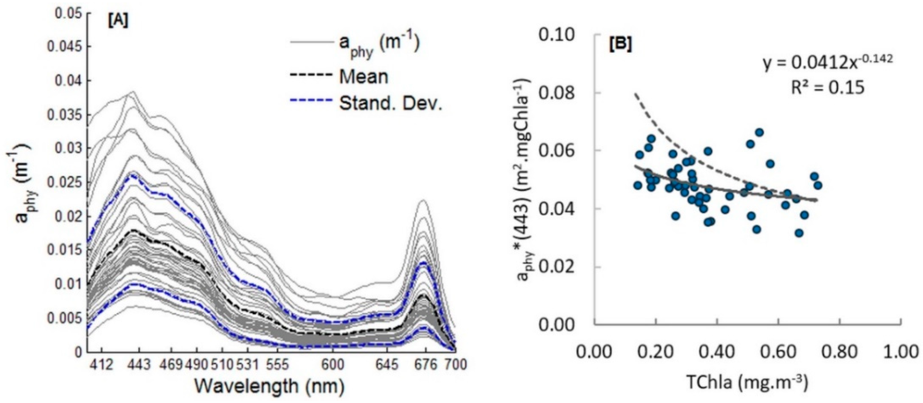
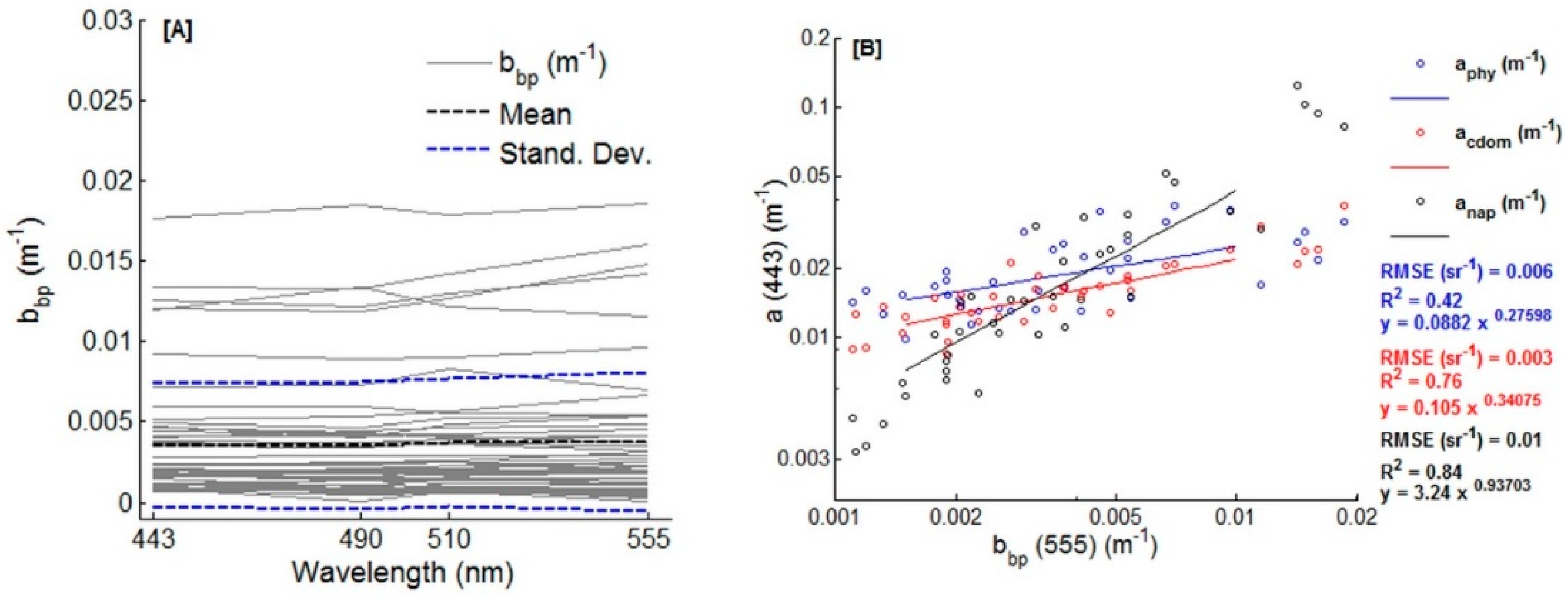
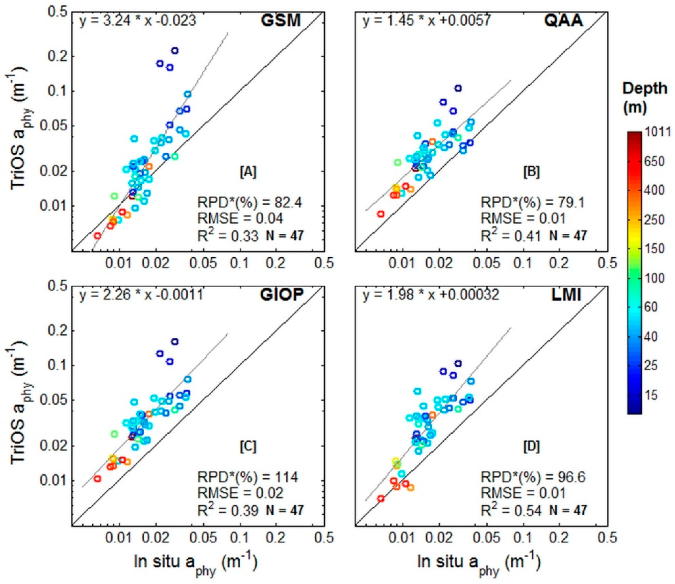
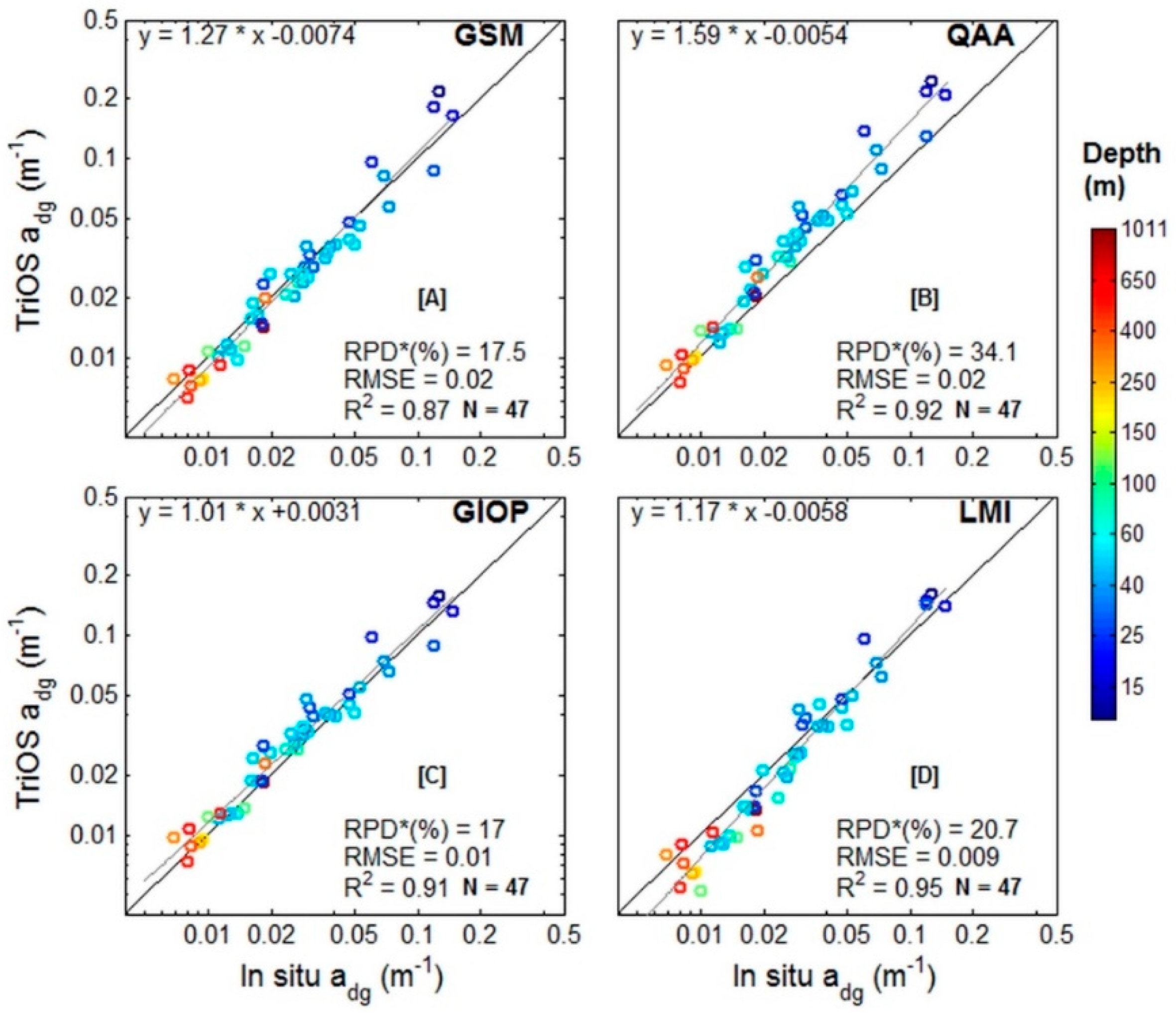
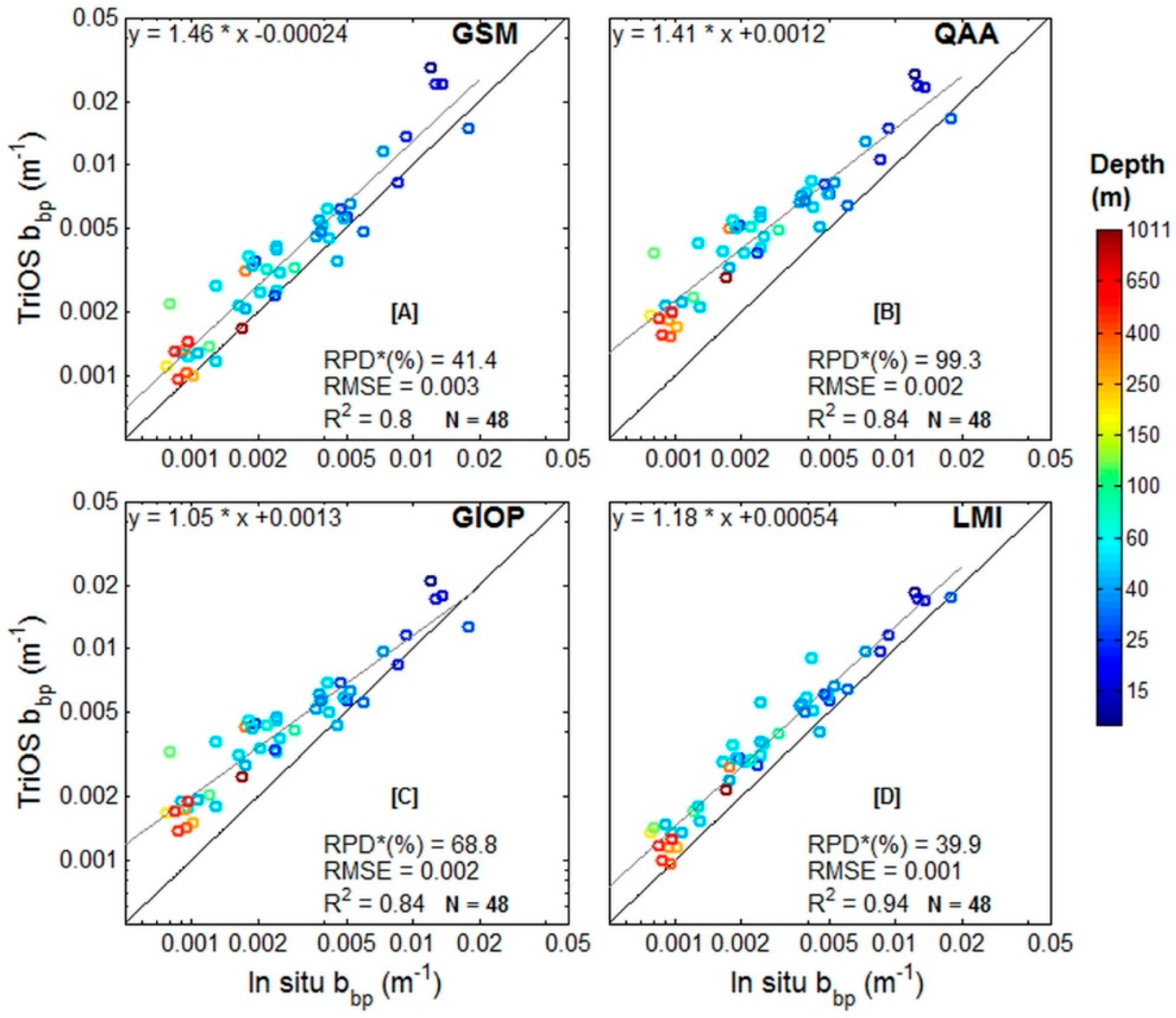
3.3.2. Inherent Optical Properties

The semi-analytical algorithms have the advantage of inverting the IOPs i.e., a_phy, a_dg, and b_bp, simultaneously or quasi-simultaneously, within some steps. Hence, for optically complex waters with mixture of different constituents that vary independently, from different sources, these approaches should be more suitable. The problem is that with a greater number of unknown parameters and variables, the solution also becomes more complex and subject to higher uncertainty, when each parameter is not appropriately adjusted. Hence, uncertainties in the parameterization of each of the specific IOPs will propagate to all the IOPs through spectral compensations effects. What differentiates each of the algorithms, besides of the mathematical approach of the inversion scheme, is how they deal with the parameterization of the specific IOPs, either by setting an optimized average i.e., GSM and LMI, or using empirical functions to account for at least for some of the specific optical variability, i.e., GIOP and QAA.

For the a_phy(443) inversion, the GSM01 and GIOP showed basically the same performance as for the Chla retrievals, and the sources of uncertainty are similar to those previously cited, i.e., spectral mixture with higher NAP and CDOM contributions at the coastal stations, a_phy* variability, and spectral compensations effects with the bulk IOP inversion. The GSM had an overall percent difference of 75% with both under (at deeper stations) and over estimations (at coastal stations) of a_phy(443), with a positive slope of 3.2, R² = 0.33 and RMSE = 0.04 m⁻¹ (Figure 12). The GIOP overestimated a_phy(443) at all of the stations with 114% RPD, 2.3 slope, R² = 0.39 and RMSE = 0.02 m⁻¹.

The QAA retrievals showed a similar dispersion as the GIOP a_phy(443), as both approaches use the same parameterization for some specific IOPs, (S_dg and S_bbp) [30,32]. However, the QAA had somewhat better retrievals for the coastal stations, resulting in a lower overall percent difference with 79%, RMSE = 0.01 m⁻¹, R² = 0.41 and a slope of 1.45 (Figure 12). The QAAv5 is in fact adjusted for application to a wide range optical water types from oceanic to coastal waters, as it uses not only blue and green R_rs bands, but also red bands in the parameterization and inversion scheme. All of the QAA spectral parameters, including the a_phy(443), are empirically derived using a blue:green R_rs band ratio for each inversion [30], which may have also contributed for the improved a_phy(443) retrievals, although local variations in a_phy* and spectral mixture of NAP and CDOM still posed some challenges.

The LMI a_phy(443) retrievals had a distribution similar to the QAA retrievals (with a lower slope of 1.98), but a higher mean percent difference (97%). There was a good agreement for the deepest stations, and overestimations for the coastal stations. The regional adjustment uses an average a_phy*(443) of 0.05 m²·mgChla⁻¹, due to the dominance of nanoplankton cells in the New Caledonia coastal lagoons [36,37]. This value was very close to the in situ measurements obtained for the deeper stations, which may explain the best fit in this case, but was somewhat higher than the a_phy*(443) of the coastal stations. The positive biases, in this case, could be due to the higher spectral mixture and overestimation of the other IOPs (such as b_bp(443), as will be further shown).

As for the Chla retrievals, the stations with highest a_phy(443) biases for all algorithms (>100% RPD) were the ones in which a_dg(443) contributed to more than 80% of the total non-water light absorption. Taking out these stations the overall biases reduces to 40% for the GSM, 60% for the QAA and, 70% for the LMI.

The optical dominance of NAP and CDOM absorption in the ELNC waters, on the other hand, favoured the retrieval of a_dg(443) by all algorithms, yielding the lowest percent differences i.e., 17–34% (Figure 13). The GSM01 retrievals had a similar distribution as the LMI (1.27 and 1.17 slope), as both algorithms use a a_dg spectral slope of 0.020 nm⁻¹. The in situ measurements, however, showed a lower average a_dg spectral slope of 0.014 nm⁻¹, which may partly explain the negative biases.

The GIOP (by default) and QAA, both use the a_dg spectral slope obtained by an empirical relation with the blue:green R_rs band ratio for each station [32]. In this case, the values used for these algorithms were much closer to the in situ measurements i.e., 0.015–0.020 nm⁻¹, with a mean of 0.016 nm⁻¹. Lower S_dg used to invert a_dg(443) may, however, have favoured some of the positive biases due to the imprecise parameterization of the other specific IOPs, during the bulk inversion. It is worth noting here, that even though there were some deviations between the parameterized S_dg and in situ measurements, especially for the GSM01 and LMI, uncertainties due to local variations in this specific IOP, seemed to have minor impacts on the retrieved a_dg(443).

For the b_bp(443) inversion, the GSM01 and LMI gave the best performance with the lowest percent differences i.e., ~40%, and high covariation (0.8–0.9 R²). The GIOP and QAA retrievals showed similar distributions with higher overestimations at the deepest stations, and an overall percent difference of 69% and 99%, respectively (Figure 14). All the algorithms were mostly positively biased, which may be somewhat due to the higher b_bp spectral slope used to parameterize each of them. The GSM01 uses a global optimized b_bp spectral slope of 1.03 nm⁻¹ and regional LMI of 1.0 nm⁻¹, which were somewhat higher than the in situ measurements (mean, 0.07 nm⁻¹). The GIOP (by default) and QAA both use an empirical function relating R_rs band ratios to estimate S_bbp [32]. In this case, however, the retrieved values were even higher than the in situ measurements, with an average of 1.38 nm⁻¹. This may explain the higher positive biases obtained for these two approaches.

Besides of the biases related to imprecise parameterization of S_bbp and spectral compensation effects within the inversion process, the b_bp(443) retrievals are more impacted by slight variations in the R_rs at the longer bands. Hence, part of the positive biases could be related to the R_rsT(555) positive biases due to bubble cloud effects, in-water structure reflection, as well as Raman scattering, as discussed in Section 3.2.2. Inversion algorithms that do not take into account Raman scattering, can have up to 50% positive biases for the b_bp(443) retrievals in waters with 0.1–0.5 mg·m⁻³ of Chla [83].

In summary, all algorithms need improvements to properly invert the a_phy(443) (and Chla) in the ELNC, but they all showed a good performance for a_dg(443) and reasonable agreement for b_bp(443), especially GSM01 and LMI. The GSM01 and LMI algorithms provided very similar performance due to the close values used for the global and regional parameterizations of the specific IOPs. The GIOP and QAA, despite the more versatile parameterization scheme applicable to a wide range of optical water types, had some significant deviations, due to more complex regional-local variability of the specific optical properties at the ELNC. As discussed by Mukarami and Dupouy [37], due to the relatively high spatial-temporal variability of the specific IOPs at the ELNC waters, improvements in the inversion of the IOPs may potentially be achieved by applying an optical water type parameterization scheme rather than an average regional parameterization.

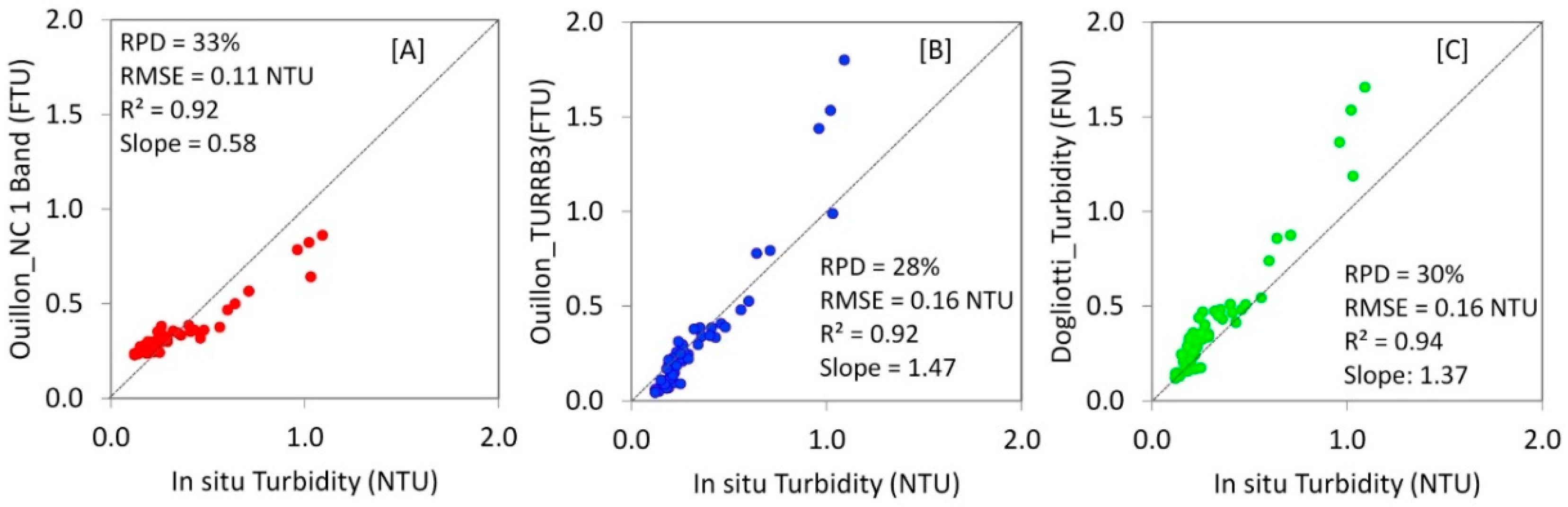
3.3.3. Water Turbidity

For surface water turbidity the three approaches that were applied to the ELNC i.e., the regional and global empirical algorithms of Ouillon et al. [38] and the single semi-analytical algorithm of Dogliotti et al. [39], showed a reasonable performance for optically deep waters (i.e., without bottom influence), with the RPD around 30%, and a high co-variation between estimated and measured turbidity (R²~0.92) (Figure 15). The regional algorithm adjusted for New Caledonia coastal waters (Figure 15A) had positive biases for the clearest waters and negative biases for turbidity above 0.2 NTU (slope, 0.58). The positive biases were obtained for the values out of the algorithm range of applicability, since the lowest turbidity used to calibrate the algorithm was 0.2 FTU [38]. This a limitation of purely empirical approaches which cannot deal with values out of their range of applicability. Above 0.2 NTU, the underestimation was rather systematic error, which is typical of measurement biases. As the regional approach uses a one-band empirical relation between R_rs(565) and water turbidity (<1 FTU), it can be highly influenced by biases in the remote sensing reflectance. Hence, differences in the R_rs used to calibrate and apply the algorithm can significantly impact the performance of this approach. Ouillon et al. [38] obtained the in situ R_rs with above-water instrumentation (Ocean Optics USB2000), using a surface reflectance factor [86] to correct for the contribution of skylight radiance reflected from the ocean surface. These measurements however, are known to have residual uncorrected sky and sun glint signals manifested by a positive (approximately white) spectral shift [14,61]. This positive bias in the above-water R_rs can be corrected using simple white offset corrections for waters where null near-medium-infrared water reflectance can be assumed [61], or using more elaborated correction schemes for turbid waters [87]. Such residual correction was not performed by Ouillon et al. [38], which may explain the negative biases of the algorithm when applying R_rs obtained by in-water approaches as for the ELNC in the present work.

The global empirical algorithm developed by Ouillon et al. [38] for tropical coastal waters uses a two-step scheme with a 3-band ratio algorithm (R_rs(620). R_rs(681)/R_rs(412)) to estimate turbidity below 1 FTU, and a one-band algorithm (R_rs(618)) for turbidity from 1 to 25 FTU. All of the ELNC cases fell into the 3-band ratio algorithm criteria and had a different distribution than the regional algorithm (Figure 15A,B). For the cases below the range of applicability (<0.2 NTU), the global algorithm underestimated the water turbidity, and for most of the cases between 0.2 and 1 FTU the global algorithm had an improved performance compared to the regional approach. This is because the band ratio of the global approach minimizes spectrally correlated biases related to the R_rs. The drawback is that the selected band ratio is sensitive to changes in the particle composition, as well as dissolved absorbing constituents, i.e., CDOM, which impact the R_rs(412). Hence, higher absorption of CDOM and NAP, due to a higher fraction of organic compounds in the particle assemblage, will cause turbidity overestimations for this approach. This may explain the high overestimations obtained for the 3 stations that deviated more than 50% (stations 14, 20 and 24, Figure 15B). These stations were located near rivers and mining sites, and the presence of dissolved and adsorbed iron, leached from iron-rich ultramafic soils (in New Caledonia) [51], may have also contributed to the higher light absorption in the shorter bands and turbidity overestimation. If a smoothed transition between the application of Equations (1) and (2) was made, using a weighted average for instance, the retrieved turbidity would be much closer to the observed one, reducing RPD to 18% for these 3 stations. The use of R_rs(681) to estimate turbidity is however questionable, since this band is located near the chlorophyll a in vivo fluorescence peak, and uncorrelated changes in phytoplankton fluorescence will affect the turbidity estimation. Although the 3-band approach provided the best results for Ouillon et al. [38], and showed a reasonably good performance for the ELNC, the applicability of this approach needs to be analysed with caution due to all these potential sources of uncertainty.

The Dogliotti et al. [39] single algorithm was proposed to solve or at least minimize these sources of uncertainty with a one-band semi-analytical algorithm for all water types i.e., ρ(645) for 0–15 FNU and ρ(859) for 15–1000 FNU. In fact, even being parameterized with data collected from various sites, including a wide range of optical water types, the overall performance of this approach was reasonably good and similar to the Ouillon et al. [38] empirical algorithm for tropical waters (<25 FTU), i.e., 30% RPD, 0.16 FNU RMSE, 0.94 R² and 1.37 slope (Figure 15C). The semi-analytical approach improved the retrievals for the clearest waters (>0.2 NTU) and had an overall tendency to overestimate turbidity. The positive biases in this case could be related to the positive biases in the R_rs used for the application, as the one-band approach is more sensitive to slight variations in R_rs. As discussed in Section 3.2 the TriOS in-water measurements seemed to be more subjected to positive biases at the longer bands i.e., 24% positive bias of R_rsT compared to R_rsS at 645 nm, likely due to bubble clouds and in-water reflection. Raman scattering may also play a role as a source of positive bias for turbidity retrievals in clear waters, as it affects b_bp retrievals in inversion algorithms [83].

Another important source of uncertainty is related to the turbidity measurements using different methods and instrumentation. Optical turbidity measurements that use a broad band and different scattering angles are more influenced by variations in the particle composition, and the relation between turbidity and b_bp can vary by a factor of 2 [88]. Other sources that may account for up to 10% of uncertainty in the turbidity algorithm are related to variations in the scattering phase function (SPF) and bidirectional effects on the R_rs. These however, were likely minor for the ELNC since there is typically a lower variability in SPF for relatively clear waters, and nadir R_rs measurements are less subject to bidirectional effects [39]. Finally, vertical stratification can also be a source of uncertainty in the turbidity retrievals, especially for the coastal stations, which are typically more stratified. Considering all these possible sources of uncertainty and the low range of turbidity measured in the ELNC during CALIOPE 2 (0.1–1.09 NTU), the surface water turbidity was reasonably well retrieved by the tested algorithms, encouraging their application to satellite ocean monitoring of ELNC waters, without bottom influence, and/or with proper bottom reflectance corrections on the surface R_rs [36,37].

4. Conclusions and Final Remarks

The East Lagoon of New Caledonia, a tropical semi-enclosed lagoon surrounded by a coral reef barrier, has oligo-mesotrophic waters containing a variety of optically active constituents, i.e., phytoplankton, coloured dissolved organic matter, and organic and inorganic non-algal particles. These constituents vary in concentration and optical properties, with different contributing sources, i.e., oligotrophic oceanic water intrusions across the reef barrier (especially in the southern and northern tips), and continental drainage along the coast. CDOM and NAP have various sources, from small and medium river inputs, coastal erosion at mining sites, sediment re-suspension at shallower depths (<20 m), as well as releases from the coral reef ecosystem, besides the autochthonous sources from the phytoplankton community. These different sources provide a complex mixture of inherent optical properties for the ELNC waters, which vary spatially and temporally according to the seasons.

The average Chla (and maximum value) observed during CALIOPE 2, end of the austral summer of 2014 (i.e., mean, 0.37 mg·m⁻³ and maximum 0.725 mg·m⁻³), was somewhat higher than the observed during CALIOPE 1 (mean, 0.21 mg·m⁻³ and maximum 0.6 mg·m⁻³) in the dry and calm winter season of 2011, and lower than during the CALIOPE 3 (mean, 0.37 mg·m⁻³ and maximum 3.51 mg·m⁻³), summer of 2016, which was more influenced by the rainy season. Even with the late rainy season, there was still a relatively high amplitude of variability of the IOPs during CALIOPE 2, which was also influenced by wind-induced resuspension processes, i.e., 0.007–0.037 m⁻¹ for a_phy(443), 0.001–0.10 m⁻¹ for a_nap(443), 0.004–0.037 m⁻¹ for a_cdom(443), and 0.004–0.018 m⁻¹ for b_bp(443), associated to the concentration of the optical constituents from the different autochthonous and allochthonous contributing sources. There were also some important “local” variations in the specific optical properties. The phytoplankton specific absorption coefficient was generally lower than typical values observed for the corresponding Chla range across the oceans (mean, 0.049 m²·mgChla⁻¹), likely due to photo-adaptation processes. The spectral slopes of a_dg (mean, 0.016 nm⁻¹) and b_bp (mean, 0.07 nm⁻¹) were also lower than global mean values used to parameterize semi-analytical ocean colour algorithms, likely due to the higher contributions of NAP, including inorganic sediments from iron-rich eroded soil due to the mining activities.

Ocean colour radiometric measurements by the in-water instruments were in reasonable agreement (<20% RPD for R_rs(412–555)), despite the generally adverse environmental conditions of variable cloud cover, some high solar zenith angles, and relatively strong winds (mean speed: 8.5 m⁻¹). An adapted floating PVC structure attached to the TriOS in-water sensor, allowed data collection away from the vessel to avoid platform shading effects, therefore improving the match-ups between R_rs(412–555) obtained by the free-falling Satlantic profiler. Minor uncertainties likely associated to self-shading effects, bubble clouds, and reflection by ship structures remained, especially for the TriOS approach, due to the range of optical water types and rough sea conditions sampled during CALIOPE 2. These adverse conditions posed higher challenges for the closure experiment, but still differences were lower than those observed in other works (<26% RPD for R_rs(443-555)), encouraging the use of the adapted TriOS in-water approach. A potential source of difference in the measured and modelled R_rs is also due to Raman scattering, which may explain some of the negative RTE R_rs biases. When applying the bio-optical algorithms the R_rsT uncertainties should have caused higher impacts on the IOP retrievals at the clearest waters, with overestimations for all IOPs. Such impacts were minor for the Chla and absorption coefficients, as the positive biases were obtained mostly at the coastal turbid stations. For the b_bp(443) retrievals, however, positive R_rs biases and ignoring Raman scattering likely contributed to the positive b_bp biases obtained in all cases.

The GSM01 provided the best overall performance inverting the Chla and a_phy(443) with 35% RPD, (excluding the most turbid coastal stations), the a_dg(443) with 18% RPD (for all cases), and the b_bp(443) with 40% RDP. For a globally tuned algorithm applied to a coastal lagoon, with optically complex waters, this algorithm performed reasonably well, and may be applied to monitor the ELNC waters, with caution only for the Chla and a_phy(443) retrievals in the most turbid waters (>1 NTU) with higher spectral mixture. The QAA also provided reasonably good retrievals and was particularly better for the a_phy(443) inversion at the coastal turbid stations. The GIOP and LMI showed potential for an improved performance if site-specific parameterizations for the a_phy*, S_dg, and b_bp spectral slopes are applied. The regionally tuned LMI, however, revealed the challenge of how to select the best parameterization, as the regional algorithm still did not properly capture spatiotemporal variations in the specific IOPs of the ELNC. An optical water type parameterization scheme could be an alternative and needs further investigation.

The global and regional water turbidity algorithms showed promising results for satellite ocean colour applications, with biases mostly related to the R_rs and turbidity measurements used for each adjustment, and particle type variability that may still leave some residual biases depending on the approach and methods used. The global single algorithm proposed by Dogliotti et al. [39] seems to be the most robust approach applicable for all water types, independent of the particle assemblage and for a wide range of turbidity (0–1000 FNU), if provided with high quality R_rs or ρ values; it performed similarly to the Ouillon et al. [38] algorithm for tropical waters on the CALIOPE 2 data. Surface water turbidity is an important parameter to monitor in the ELNC, especially to analyse the impacts of river runoff after intensive rainy events and soil erosion at the mining sites [42], as the increased water turbidity can have severe consequences for the coral reef ecosystem.

Future works should gather all the data sets from the CALIOPE cruises across the ELNC, to fully characterize the spatial and temporal bio-optical variability under different scenarios (e.g., dry and wet seasons), and to build a robust database for appropriate parameterizations of the ocean colour algorithms (regional/seasonal or class-based). With proper parameterizations ocean colour products may then be used to monitor the biogeochemical properties at the ELNC and detect changes in this highly vulnerable marine ecosystem.

References

1. NOAA’S. Coral Reef Conservation Program: Coastal Protection. 2011. Available online: http://coralreef.noaa.gov/aboutcorals/values/coastalprotection/ (accessed on 22 May 2014).
2. Payri, C.; Benzoni, F.; Houlbreque, F. Le blanchissement des coraux: L’épisode de 2016 en Nouvelle Calédonie. l’ENA hors les murs 2017, 470, 13–16. [Google Scholar]
3. Hoegh-Guldberg, O.; Mumby, P.J.; Hooten, A.J.; Steneck, R.S.; Greenfield, P.; Gomez, E.; Harvell, C.D.; Sale, P.F.; Edwards, A.J.; Caldeira, K.L.; et al. Coral reefs under rapid climate change and ocean acidification. Science 2007, 318, 1737–1742. [Google Scholar] [CrossRef] [PubMed]
4. Diaz-Pulido, G.; Gouezo, M.; Tilbrook, B.; Dove, S.; Anthony, K.R.N. High CO2 enhances the competitive strength of seaweeds over corals. Ecol. Lett. 2011, 14, 156–162. [Google Scholar] [CrossRef] [PubMed]
5. Courtial, L.; Ferrier-Pages, C.; Jaquet, S.; Houlbreque, F. Effects of temperature and UVR on organic matter fluxes and the metabolic activity of Acropora muricata. Biol. Open 2017, 6, 1190–1199. [Google Scholar] [CrossRef] [PubMed]
6. Andrefouët, S.; Payri, C.; Van Wynsberge, S.; Lauret, O.; Alefaio, S.; Preston, N.G.; Yamano, H.; Baudel, S. The timing and the scale of the proliferation of Sargassum polycystum in Funafuti Atoll, Tuvalu. J. Appl. Phycol. 2017, 29, 3097–3108. [Google Scholar] [CrossRef]
7. IUCN. The Lagoons of New Caledonia: Reef Diversity and Associated Ecosystems (France); Evaluation Report; World Heritage Committee IUCN: Gland, Switzerland, 2008; pp. 43–54. [Google Scholar]
8. Dupouy, C.; Lefèvre, J.; Wattelez, G.; Martias, C.; Andreoli, R.; Lille, D. Satellite survey of lagoons and reefs. In Récifs Calédoniens; IFRECOR: Roubaix, France, 2018. [Google Scholar]
9. Dupouy, C.; Röttgers, R.; Tedetti, M.; Martias, C.; Murakami, H.; Doxaran, D.; Lantoine, F.; Rodier, M.; Favareto, L.R.; Kampel, M.; et al. Influence of CDOM and particle composition on ocean color of the Eastern New Caledonia Lagoon during the CALIOPE cruises. In Ocean Remote Sensing and Monitoring from Space; 92610M; International Society for Optics and Photonics: Bellingham, WA, USA, 2014; Volume 9261. [Google Scholar] [CrossRef]
10. Martias, C.; Tedetti, M.; Lantoine, F.; Jamet, L.; Dupouy, C. Characterization and sources of colored dissolved organic matter in a coral reef ecosystem subject to ultramafic erosion pressure (New Caledonia, Southwest Pacific). Sci. Total Environ. 2018, 616–617, 438–452. [Google Scholar] [CrossRef] [PubMed]
11. Eakin, C.M.; Nim, C.J.; Brainard, R.E; Aubrecht, C.; Elvidge, C.; Gledhill, D.K.; Muller-Karger, F.; Mumby, P.J.; Skirving, W.J.; Strong, A.E.; et al. Monitoring coral reefs from space. Oceanography 2010, 23, 118–133. [Google Scholar] [CrossRef]
12. Mouw, C.B.; Greb, S.; Aurin, D.; DiGiacomo, P.M.; Lee, Z.; Twardowski, M.; Binding, C.; Hu, C.; Ma, R.; Moore, T.; et al. Aquatic color radiometry remote sensing of coastal and inland waters: Challenges and recommendations for future satellite missions. Remote Sens. Environ. 2015, 160, 15–30. [Google Scholar] [CrossRef]
13. Werdell, P.J.; Bailey, S.W. An improved in-situ bio-optical data set for ocean color algorithm development and satellite data product validation. Remote Sens. Environ. 2005, 98, 122–140. [Google Scholar] [CrossRef]
14. Toole, D.A.; Siegel, D.A.; Menzies, D.W.; Neumann, M.J.; Smith, R.C. Remote-sensing reflectance determinations in the coastal ocean environment: Impact of instrumental characteristics and environmental variability. Appl. Opt. 2000, 39, 456–469. [Google Scholar] [CrossRef] [PubMed]
15. Hooker, S.B.; Maritorena, S. An evaluation of oceanographic radiometers and deployment methodologies. J. Atmos. Ocean. Technol. 2000, 17, 811–830. [Google Scholar] [CrossRef]
16. Mitchell, B.G.; Kahru, M.; Wieland, J.; Stramska, M. Determination of spectral absorption coefficients of particles, dissolved material and phytoplankton for discrete water samples. In Ocean Optics Protocols for Satellite Ocean Color Sensor Validation, Revision 4; National Aeronautical and Space Administration, Goddard Space Flight Center, NASA: Greenbelt, MD, USA, 2003; Chapter 4; Volume 4, pp. 39–60. [Google Scholar]
17. Twardowski, M.S.; Claustre, H.; Freeman, S.A.; Stramski, D.; Huot, Y. Optical backscattering properties of the “clearest” natural waters. Biogeosciences 2007, 4, 1041–1058. [Google Scholar] [CrossRef]
18. Röttgers, R.; Doxaran, D.; Dupouy, C. Quantitative filter technique measurements of spectral light absorption by aquatic particles using a portable integrating cavity absorption meter (QFT-ICAM). Opt. Express 2016, 24, A1–A20. [Google Scholar] [CrossRef] [PubMed]
19. IOCCG. Remote Sensing of Inherent Optical Properties: Fundamentals, Tests of Algorithms, and Applications, 5th ed.; Reports of the International Ocean-Colour Coordinating Group: Dartmouth, NS, Canada, 2006; p. 124. [Google Scholar]
20. Gitelson, A.A.; Schalles, J.F.; Hladik, C.M. Remote chlorophyll-a retrieval in turbid, productive estuaries: Chesapeake Bay case study. Remote Sens. Environ. 2007, 109, 464–472. [Google Scholar] [CrossRef]
21. Dall’Olmo, G.; Gitelson, A.A. Effect of bio-optical parameter variability on the remote estimation of chlorophyll-a concentration in turbid productive waters: Experimental results. Appl. Opt. 2005, 44, 412–422. [Google Scholar] [CrossRef] [PubMed]
22. O’Reilly, J.E.; Maritorena, S.; Siegel, D.A.; O’Brien, M.C.; Toole, D.; Mitchell, B.G.; Kahru, M.; Chavez, F.P.; Strutton, P.; Cota, G.F.; et al. Ocean color chlorophyll a algorithms for SeaWiFS, OC2, and OC4: Version 4. In SeaWiFS Postlaunch Technical Report Series; v.11; SeaWiFS Postlaunch Calibration and Validation Analyses, Part 3; Hooker, S.B., Firestone, E.R., Eds.; NASA, Goddard Space Flight Center: Greenbelt, MD, USA, 2000; pp. 9–23. [Google Scholar]
23. Bricaud, A.; Morel, A.; Babin, M.; Allali, K.; Claustre, H. Variations of light absorption by suspended particles with chlorophyll a concentration in oceanic (case 1) waters: Analysis and implications for bio-optical. J. Geophys. Res. 1998, 103, 31033–31044. [Google Scholar] [CrossRef]
24. Ciotti, A.M.; Lewis, M.R.; Cullen, J.J. Assessment of the relationships between dominant cell size in natural phytoplankton communities and the spectral shape of the absorption coefficient. Limnol. Oceanogr. 2002, 47, 404–417. [Google Scholar] [CrossRef] [Green Version]
25. Loisel, H.; Nicolas, J.M.; Sciandra, A.; Stramski, D.; Poteau, A. Spectral dependency of optical backscattering by marine particles from satellite remote sensing of the global ocean. J. Geophys. Res. 2006, 111, C09024. [Google Scholar] [CrossRef]
26. Siegel, D.A.; Maritorena, S.; Nelson, N.B. Global distribution and dynamics of colored dissolved and detrital organic materials. J. Geophys. Res. 2002, 107, 1–14. [Google Scholar] [CrossRef]
27. Garver, S.A.; Siegel, D.A. Inherent optical property inversion of ocean color spectra and its biogeochemical interpretation. I. Time series from the Sargasso Sea. J. Geophys. Res. 1997, 102, 18607–18625. [Google Scholar] [CrossRef]
28. Maritorena, S.; Siegel, D.A.; Peterson, A.R. Optimization of a semianalytical ocean color algorithm for global-scale applications. Appl. Opt. 2002, 41, 2705–2714. [Google Scholar] [CrossRef] [PubMed]
29. Gordon, H.R.; Brown, O.B.; Evans, R.H.; Brown, J.W.; Smith, R.C.; Baker, K.S.; Clark, D.K. A Semianalytic Radiance Algorithm of Ocean Color. J. Geophys. Res. 1988, 93, 10909–10924. [Google Scholar] [CrossRef]
30. Lee, Z.; Carder, K.L.; Arnone, R.A. Deriving inherent optical properties from water color: A multiband quasi-analytical algorithm for optically deep waters. Appl. Opt. 2002, 41, 5755–5772. [Google Scholar] [CrossRef] [PubMed]
31. Lee, Z.; Weidemann, A.; Kindle, J.; Arnone, R.; Carder, K.L.; Davis, C. Euphotic zone depth: Its derivation and implication to ocean-color remote sensing. J. Geophys. Res. 2007, 112, C03009. [Google Scholar] [CrossRef]
32. Werdell, P.J.; Franz, B.A.; Bailey, S.W.; Feldman, G.C.; Boss, E.; Brando, V.E.; Dowell, M.; Hirata, T.; Lavender, S.J.; Lee, Z.; et al. Generalized ocean color inversion algorithm for retrieving marine inherent optical properties. Appl. Opt. 2013, 52, 2019–2037. [Google Scholar] [CrossRef] [PubMed]
33. Hoge, F.E.; Lyon, P.E. Satellite retrieval of inherent optical properties by linear matrix inversion of oceanic radiance algorithms: An analysis of algorithm and radiance measurement errors. J. Geophys. Res. 1996, 101, 16631–16648. [Google Scholar] [CrossRef]
34. Hoge, F.E.; Lyon, P.E. Spectral parameters of inherent optical property models: Methods for satellite retrieval by matrix inversion of an oceanic radiance model. Appl. Opt. 1999, 38, 1657–1662. [Google Scholar] [CrossRef] [PubMed]
35. Lyon, P.; Hoge, F. The linear matrix inversion algorithm. In Remote Sensing of Inherent Optical Properties: Fundamentals, Tests of Algorithms, and Applications; IOCCG Report Number 5; Lee, Z., Ed.; International Ocean-Colour Coordinating Group (IOCCG): Monterey, CA, USA, 2006; Chapter 7; pp. 49–56. [Google Scholar]
36. Murakami, H.; Dupouy, C.; Roettgers, R.; Frouin, J.R. Estimation of inherent optical properties using in-situ hyperspectral radiometer and MODIS along the east coast of New Caledonia. In Remote Sensing of the Marine Environment II; SPIE: Bellingham, WA, USA, 2012. [Google Scholar] [CrossRef]
37. Murakami, H.; Dupouy, C. Atmospheric correction and inherent optical property estimation in the southwest New Caledonia lagoon using AVNIR-2 high-resolution data. Appl. Opt. 2013, 52, 182–198. [Google Scholar] [CrossRef] [PubMed]
38. Ouillon, S.; Douillet, P.; Petrenko, A.; Neveux, J.; Dupouy, C.; Froidefond, J.M.; Andréfouët, S.; Muñoz-Caravaca, A. Optical Algorithms at Satellite Wavelengths for Total Suspended Matter in Tropical Coastal Waters. Sensors 2008, 8, 4165–4185. [Google Scholar] [CrossRef] [PubMed] [Green Version]
39. Dogliotti, A.; Ruddick, K.G.; Nechad, B.; Doxaran, D.; Knaeps, E. A single algorithm to retrieve turbidity from remotely sensed data in all coastal and estuarine waters. Remote Sens. Environ. 2015, 156, 157–168. [Google Scholar] [CrossRef]
40. Dupouy, C.; Savranski, T.; Lefevre, J.; Despinoy, M.; Mangeas, M.; Fuchs, R.; Faure, V.; Ouillon, S.; Petit, M. Monitoring Optical Properties of the Southwest Tropical Pacific. In Remote Sensing of the Coastal Ocean, Land, and Atmosphere Environment; Frouin, R.J., Yoo, H.R., Won, J.-S., Feng, A., Eds.; SPIE: Bellingham WA, USA, 2010; Volume 7858, p. 14. [Google Scholar] [CrossRef]
41. Dupouy, C.; Neveux, J.; Ouillon, S.; Frouin, R.; Murakami, H.; Hochard, S.; Dirberg, G. Inherent optical properties and satellite retrieval of chlorophyll concentration in the lagoon and open ocean waters of New Caledonia. Mar. Pollut. Bull. 2010, 61, 503–518. [Google Scholar] [CrossRef] [PubMed]
42. Dupouy, C.; Frouin, R.; Röttgers, R.; Neveux, J.; Gallois, F.; Panché, J.Y.; Gerard, P.; Fontana, C.; Pinazo, C.; Ouillon, S.; et al. Ocean Color Response to an Episode of Heavy Rainfall in the Lagoon of New Caledonia. In Proceedings of the SPIE Conference Ocean Remote Sensing: Methods and Applications, San Diego, CA, USA, 19 August 2009; Volume 7459. [Google Scholar] [CrossRef]
43. Neveux, J.; Tenório, M.B.; Jacquet, S.; Torréton, J.P.; Douillet, P.; Ouillon, S.; Dupouy, C. Chlorophylls and phycoerythrins as markers of environmental forcings including cyclone Erica effect (March 2003) on phytoplankton in the southwest lagoon of New Caledonia and oceanic adjacent area. Int. J. Oceanogr. 2009, 2009, 19. [Google Scholar] [CrossRef]
44. Neveux, J.; Lefebvre, J.P.; Le Gendre, R.; Dupouy, C.; Gallois, F.; Courties, C.; Gérard, P.; Fernandez, J.M.; Ouillon, S. Phytoplankton dynamics in New Caledonian lagoon during a southeast trade winds event. J. Mar. Syst. 2010, 82, 230–244. [Google Scholar] [CrossRef]
45. Röttgers, R.; Dupouy, C.; Taylor, B.; Bracher, A.; Wozniak, S. Mass-specific light absorption coefficients of natural aquatic particles in the near-infrared spectral region. Limnol. Oceanogr. 2014, 59, 1449–1460. [Google Scholar] [CrossRef] [Green Version]
46. Wattelez, G.; Dupouy, C.; Mangeas, M.; Lefèvre, J.; Touraivane; Frouin, J.R. A Statistical Algorithm for Estimating Chlorophyll Concentration in the New Caledonian Lagoon. Remote Sens. 2016, 8, 45. [Google Scholar] [CrossRef] [Green Version]
47. Fuchs, R.; Pinazo, C.; Douillet, P.; Fraysse, M.; Grenz, C.; Mangin, A.; Dupouy, C. Modelling the ocean-lagoon interaction via upwelling processes on the South West of New Caledonia. Estuar. Coast. Shelf Sci. 2013, 135, 5–17. [Google Scholar] [CrossRef]
48. Minghelli-Roman, A.; Dupouy, C. Influence of water column chlorophyll concentration on bathymetric estimations in the lagoon of New Caledonia using several MERIS images. IEEE J. Sel. Top. Appl. Earth Obs. Remote Sens. 2013, 77, 1–7. [Google Scholar] [CrossRef] [Green Version]
49. Minghelli-Roman, A.; Dupouy, C. Seabed mapping in the lagoon of New Caledonia with MeRIS images. IEEE J. Sel. Top. Appl. Earth Obs. Remote Sens. 2014, 7, 2619–2629. [Google Scholar] [CrossRef]
50. Cravatte, S.; Kestenare, E.; Eldin, G.; Ganachaud, A.; Lefèvre, J.; Marin, F.; Menkes, C.; Aucan, J. Regional circulation around New Caledonia from two decades of observations. J. Mar. Syst. 2015, 148, 249–271. [Google Scholar] [CrossRef]
51. Dublet, G.; Juillot, F.; Morin, G.; Fritsch, E.; Fandeur, D.; Brown, G.E., Jr. Goethite aging explains Ni depletion in upper units of ultramafic lateritic ores from New Caledonia. Geochim. Cosmochim. Acta 2015, 160, 1–15. [Google Scholar] [CrossRef] [Green Version]
52. Alory, G.; Vega, A.; Ganachaud, A.; Despinoy, M. Influence of upwelling, subsurface stratification, and heat fluxes on coastal sea surface temperature off southwestern New Caledonia. J. Geophys. Res. 2006, 111, C07023. [Google Scholar] [CrossRef]
53. Vega, A.; Ganachaud, A.; Bosson, J. Atlas Climatologique Satellite des Courants, vent, Elevation et Temperature en Surfasse dans Zone Economique Exclusive de Nouvelle-Caledonie; Elaboré par le Laboratoire d’Etudes Géophysiques et d’Océanographie Spatiale de L’Institut de Recherche pour le Développement (IRD): Nouméa, New Caledonia, 2005; pp. 1–27. [Google Scholar]
54. Maffione, R.A.; Dana, D.R. Instruments and methods for measuring the backward-scattering coefficient of ocean waters. Appl. Opt. 1997, 36, 6057–6067. [Google Scholar] [CrossRef] [PubMed]
55. Van Heukelem, L.; Thomas, C.S. Computer-assisted high-performance liquid chromatography method development with applications to the isolation and analysis of phytoplankton pigments. J. Chromatogr. 2001, 910, 31–49. [Google Scholar] [CrossRef]
56. Röttgers, R.; Doerffer, R. Measurements of optical absorption by chromophoric dissolved organic matter using a point-source integrating-cavity absorption meter. Limnol. Oceanogr. Methods 2007, 5, 126–135. [Google Scholar] [CrossRef] [Green Version]
57. Mitchell, B. Algorithms for determining the absorption coefficient for aquatic particulates using quantitative filter technique. In SPIE, Ocean Optics X; SPIE: Orlando, FL, USA, 1990; Volume 1302, p. 12. [Google Scholar] [CrossRef]
58. Tassan, S.; Ferrari, G.M. An alternative approach to absorption measurements of aquatic particles retained on filters. Limnol. Oceanogr. 1995, 40, 1358–1368. [Google Scholar] [CrossRef] [Green Version]
59. Röttgers, R.; Häse, C.; Doerffer, R. Determination of the particulate absorption of microalgae using a point-source integrating-cavity absorption meter: Verification with a photometric technique, improvements for pigment bleaching and correction for chlorophyll fluorescence. Limnol. Oceanogr. Methods 2007, 5, 1–12. [Google Scholar] [CrossRef]
60. Pope, R.; Fry, E. Absorption spectrum (380–700 nm) of pure water. II. Integrating cavity measurements. Appl. Opt. 1997, 36, 8710–8723. [Google Scholar] [CrossRef] [PubMed]
61. Mueller, J.L. Overview of radiometric measurement and data analysis methods. In Ocean Optics Protocols for Satellite Ocean Color Sensor Validation; Mueller, J.L., Fargion, G.S., McClain, C.R., Eds.; NASA: Greenbelt, MD, USA, 2003; pp. 7–20. [Google Scholar]
62. Gordon, H.R.; Mccluney, W.R. Estimation of the Depth of Sunlight Penetration in the Sea for Remote Sensing. Appl. Opt. 1975, 14, 413–416. [Google Scholar] [CrossRef] [PubMed]
63. Rudorff, N.M.; Frouin, R.; Kampel, M.; Goyens, C.; Meriaux, X.; Schieber, B.; Mitchell, B.G. Ocean-color radiometry across the Southern Atlantic and Southeastern Pacific: Accuracy and remote sensing implications. Remote Sens. Environ. 2014, 149, 13–32. [Google Scholar] [CrossRef]
64. Froidefond, J.M.; Ouillon, S. Introducing a mini-catamaran to perform reflectance measurements above and below the water surface. Opt. Express 2005, 13, 926–936. [Google Scholar] [CrossRef] [PubMed]
65. Morel, A.; Antoine, D.; Gentili, B. Bidirectional reflectance of oceanic waters: Accounting for Raman emission and varying particle scattering phase function. Appl. Opt. 2002, 41, 6289–6306. [Google Scholar] [CrossRef] [PubMed]
66. Park, Y.J.; Ruddick, K. Model of remote-sensing reflectance including bidirectional effects for case 1 and case 2 waters. Appl. Opt. 2005, 44, 1236–1249. [Google Scholar] [CrossRef] [PubMed]
67. Hénin, C.; Cresswell, G.R. Upwelling along the western barrier reef of New Caledonia. Mar. Freshw. Res. 2005, 56, 1005–1010. [Google Scholar] [CrossRef]
68. Uitz, J.; Claustre, H.; Morel, A.; Hooker, S.B. Vertical distribution of phytoplankton communities in open ocean: An assessment based on surface chlorophyll. J. Geophys. Res. 2006, 111, C08005. [Google Scholar] [CrossRef]
69. Hirata, T.; Hardman-Mountford, N.J.; Brewin, R.J.W.; Aiken, J.; Barlow, R.; Suzuki, K.; Isada, T.; Howell, E.; Hashioka, T.; Noguchi-Aita, M.; et al. Synoptic relationships between surface Chlorophyll-a and diagnostic pigments specific to phytoplankton functional types. Biogeosciences 2011, 8, 311–327. [Google Scholar] [CrossRef] [Green Version]
70. Bricaud, A.; Claustre, H.; Ras, J.; Oubelkheir, K. Natural variability of phytoplanktonic absorption in oceanic waters: Influence of the size structure of algal populations. J. Geophys. Res. 2004, 109, C11010. [Google Scholar] [CrossRef]
71. Stramski, D.; Reynolds, R.A.; Kaczmarek, S.; Uitz, J.; Zheng, G. Correction of pathlength amplification in the filter-pad technique for measurements of particulate absorption coefficient in the visible spectral region. Appl. Opt. 2015, 54, 6763–6782. [Google Scholar] [CrossRef] [PubMed]
72. Maritorena, S.; Guillocheau, N. Optical properties of the water and spectral light absorption by living and non-living particles and by yellow substances in coral reef waters of French Polynesia. Mar. Ecol. Prog. Ser. 1996, 131, 245–255. [Google Scholar] [CrossRef]
73. Bricaud, A.; Babin, M.; Claustre, H.; Ras, J.; Tièche, F. Light absorption properties and absorption budget of Southeast Pacific waters. J. Geophys. Res. 2010, 115, C08009. [Google Scholar] [CrossRef]
74. Babin, M.D.; Stramski, G.M.; Ferrari, H.; Claustre, A.; Bricaud, G.; Obolensky, N. Hoepffner Variations in the light absorption coefficients of phytoplankton, nonalgal particles, and dissolved organic matter in coastal waters around Europe. J. Geophys. Res. 2003, 108, 3211. [Google Scholar] [CrossRef]
75. Weishaar, J.L.; Aiken, G.R.; Bergamaschi, B.A.; Fram, M.S.; Fujii, R.; Mopper, K. Evaluation of specific ultraviolet absorbance as an indicator of the chemical composition and reactivity of dissolved organic carbon. Environ. Sci. Technol. 2003, 37, 4702–4708. [Google Scholar] [CrossRef] [PubMed]
76. Gordon, H.R.; Ding, K. Self-shading of in-water optical instruments. Limnol. Oceanogr. 1992, 37, 491–500. [Google Scholar] [CrossRef] [Green Version]
77. Stramski, D.; Tegowski, J. Effects of intermittent entrainment of air bubbles by breaking wind waves on ocean reflectance and underwater light field. J. Geophys. Res. 2001, 106, 345–360. [Google Scholar] [CrossRef]
78. Zibordi, G.; Berthon, J.; D’Alimonte, D. An Evaluation of Radiometric. Products from Fixed-Depth and Continuous In-Water Profile Data from Moderately Complex Waters. J. Atmos. Ocean. Technol. 2009, 26, 91–106. [Google Scholar] [CrossRef]
79. Stramska, M.; Dickey, T. Short-term variability of the underwater light field in the oligotrophic ocean in response to surface waves and clouds. Deep-Sea Res. Part I Oceanogr. Res. Pap. 1998, 45, 1393–1410. [Google Scholar] [CrossRef]
80. Green, R.E.; Sosik, H.M. Analysis of apparent optical properties and ocean color algorithms using measurements of seawater constituents in New England continental shelf surface waters. J. Geophys. Res. 2004, 109, C03026. [Google Scholar] [CrossRef]
81. Tzortziou, M.; Herman, J.R.; Gallegos, C.L.; Neale, P.J.; SubRamaniam, A.; Harding, L.W., Jr. Bio-optics of the Chesapeake Bay from measurements and radiative transfer closure. Estuar. Coast. Shelf Sci. 2006, 68, 348–362. [Google Scholar] [CrossRef]
82. Lee, Z.P.; Du, K.; Voss, K.J.; Zibordi, G.; Lubac, B.; Arnone, R.; Weidemann, A. An inherent-optical-property-centered approach to correct the angular effects in water-leaving radiance. Appl. Opt. 2011, 50, 3155–3167. [Google Scholar] [CrossRef] [PubMed]
83. Westberry, T.K.; Boss, E.; Lee, Z. Influence of Raman Scattering in ocean color inversion models. Appl. Opt. 2013, 52, 5552–5561. [Google Scholar] [CrossRef] [PubMed]
84. Loisel, H.; Lubac, B.; Dessailly, D. Effect of inherent optical properties variability on the chlorophyll retrieval from ocean color remote sensing: An in situ approach. Opt. Express 2010, 18, 20949–20959. [Google Scholar] [CrossRef] [PubMed]
85. Szeto, M.; Werdell, P.J.; Moore, T.S.; Campbell, J.W. Are the world’s oceans optically different? J. Geophys. Res. 2011, 116, C00H04. [Google Scholar] [CrossRef]
86. Mobley, C.D. Estimation of the remote-sensing reflectance from above-surface measurements. Appl. Opt. 1999, 38, 7442–7455. [Google Scholar] [CrossRef] [PubMed]
87. Ruddick, K.G.; De Cauwer, V.; Park, Y.; Moore, G. Seaborne measurements of near infrared water-leaving reflectance: The similarity spectrum for turbid waters. Limnol. Oceanogr. 2006, 51, 1167–1179. [Google Scholar] [CrossRef] [Green Version]
88. Neukermans, G. Optical In Situ and Geostationary Satellite-Borne Observations of Suspended Particles in Coastal Waters. Ph.D. Thesis, Université du Littoral–Côte d’Opale, Wimereux, France, 2012. [Google Scholar]
Figure 1. Map of the study area indicating the location of the sampling stations from the CALIOPE 2 conducted from 8 to 21 of March 2014 in the Eastern Lagoon of New Caledonia (ELNC). Data from bathymetry, hydrography, villages, and mining sites were downloaded from ftp://ftp.gouv.nc/sig/ accessed on 5 February 2014.
Remotesensing 10 01043 g001
Figure 2. Photographs of the Satlantic Hyperpro-II free-falling radiometer (A,B) and the TriOS-RAMSES in-water radiometer attached to a floating polyvinyl chloride (PVC) frame (C,D).
Remotesensing 10 01043 g002
Figure 3. Surface distribution maps of the surface water salinity (A) and turbidity (B) in the ELNC, during CALIOPE 2 (March 2014) cruises.
Remotesensing 10 01043 g003
Figure 4. Phytoplankton absorption (aphy) spectra (A) and specific phytoplankton absorption coefficient (aphy*) at 443 nm versus the TChla, with the power law regression fit (solid line) and the Bricaud et al. [23] fit for reference (dashed line) (B) (Number of samples = 52).
Remotesensing 10 01043 g004
Figure 5. Coloured dissolved organic matter (CDOM) absorption (acdom) spectra (A) and non-algal particles (NAP) absorption (anap) spectra for each station, mean and standard deviation for all stations (B) (Number of samples = 52).
Remotesensing 10 01043 g005
Figure 6. Mean (solid lines) and standard deviation (dashed lines) of phytoplankton absorption (aphy), Coloured dissolved organic matter (CDOM) absorption (acdom) and non-algal particles (NAP) absorption (anap) (A). Ternary diagram with the proportions of aphy(443), acdom(443) and anap(443) for each station (Number of samples = 51) colour coded by the bottom depth (m) (B).
Remotesensing 10 01043 g006
Figure 7. Particulate backscattering coefficient (bbp) spectra for each station, mean and standard deviation (Number of samples = 52) (A). The bbp at 555 nm versus phytoplankton absorption (aphy) at 443 nm, Coloured dissolved organic matter (CDOM) absorption (acdom) at 443 nm and non-algal particles (NAP) absorption (anap) at 443 nm with their mean square error, coefficient of determination (R2) and the power law fit for the 51 stations sampled in ELNC (B) (axes in log10).
Remotesensing 10 01043 g007
Figure 8. In situ remote sensing reflectance (Rrs) spectra obtained with the TriOS sensor (A) and the surface distribution map of Rrs(555) (B) (Number of samples = 48).
Remotesensing 10 01043 g008
Figure 9. Comparison of Remote sensing reflectance from TriOS radiometer (RrsT) vs. Remote sensing reflectance from Satlantic radiometer (RrsS) for the ocean colour bands and the 443:555 ratio (Number of samples = 34).
Remotesensing 10 01043 g009
Figure 10. Comparison of the modelled Remote sensing reflectance (Rrs) of the radiative-transfer equation (RTE) following Park and Ruddick [66] and measured Remote sensing reflectance from TriOS radiometer (RrsT) for each band and for the 443:555 band ratio (Number of samples = 48).
Remotesensing 10 01043 g010
Figure 11. Comparisons between the in situ measured and modelled chlorophyll a concentration (Chla) using Remote sensing reflectance from TriOS radiometer (RrsT) (TriOS Chla), determined with the: OC3M (A), OC4 (B), Garver-Siegel-Maritorena (GSM01) (C) and Generalized IOP (GIOP) (D) (Number of samples = 48). Axes in log scale.
Remotesensing 10 01043 g011
Figure 12. Comparisons between the in situ measured and modelled phytoplankton absorption (aphy) at 443 nm using Remote sensing reflectance from TriOS radiometer (RrsT) (TriOS aphy) obtained with: Garver-Siegel-Maritorena (GSM01) (A), Quasi-Analytical Algorithm (QAA) (B), Generalized IOP (GIOP) (C) and Linear Matrix Inversion (LMI) (D) (Number of samples = 47). Axes in log scale.
Remotesensing 10 01043 g012
Figure 13. Comparisons between the in situ measured and modelled absorption of Coloured dissolved organic matter (CDOM) plus non-algal particles (NAP), the adg at 443 nm using Remote sensing reflectance from TriOS radiometer (RrsT) (TriOS adg) obtained with: Garver-Siegel-Maritorena (GSM01) (A), Quasi-Analytical Algorithm (QAA) (B), Generalized IOP (GIOP) (C) and Linear Matrix Inversion (LMI) (D) (Number of samples = 47). Axes in log scale.
Remotesensing 10 01043 g013
Figure 14. Comparisons between the in situ measured and modelled particle backscattering coefficient (bbp) at 443 nm using Remote sensing reflectance from TriOS radiometer (RrsT) (TriOS bbp) obtained with: Garver-Siegel-Maritorena (GSM01) (A), Quasi-Analytical Algorithm (QAA) (B), Generalized IOP (GIOP) (C) and Linear Matrix Inversion (LMI) (D) (Number of samples = 47). Axes in log scale.
Remotesensing 10 01043 g014
Figure 15. Turbidity estimated following Ouillon et al. [38] for New Caledonia (A) and “global” tropical coastal waters (B) and Dogliotti et al. [39] (C), compared to turbidity measured in situ (Number of samples = 48).
Remotesensing 10 01043 g015