Dual-Polarized L-Band SAR Imagery for Temporal Monitoring of Marine Oil Slick Concentration


1
DEMR, ONERA, F-13661 Salon Air CEDEX, France
2
Université de Toulon, Aix Marseille Université, CNRS IRD, MIO UM110, La Garde, France
*
Author to whom correspondence should be addressed.
Remote Sens. 2018, 10(7), 1012; https://doi.org/10.3390/rs10071012
Submission received: 7 May 2018
/
Revised: 15 June 2018
/
Accepted: 20 June 2018
/
Published: 25 June 2018
(This article belongs to the Special Issue Oil Spill Remote Sensing)
Abstract
:SAR sensors are usually used in the offshore domain to detect marine oil slicks which allows the authorities to guide cleanup operations or prosecute polluters. As radar imagery can be used any time of day or year and in almost any weather conditions, the use and programming of such remote sensing data is usually favored over optical imagery. Nevertheless, images collected in the optical domain provide access to key information not accessible today by SAR instruments, such as the thickness or the amount of pollutant. To address this knowledge gap, a methodology based on the joint use of a scattering model (U-WCA) and remote sensing data collected by a low frequency (e.g., L-band) imaging radar over controlled release of mineral oil spill is reported in this paper. The proposed method allows estimation of the concentration of pollutant within an oil-in-water mixture as well as the temporal variation of this quantity due to weathering processes.

1. Introduction
The authorities and petroleum companies usually use airborne and spaceborne SAR (Synthetic Aperture Radar) images to detect and monitor marine slicks [1,2]. In an operational context, radar images are favored over optical ones because radar can be used any time and in almost any weather conditions [3,4,5]. In the microwave regime, the ocean surface is modelled as a set of slightly rough tilted facets that contributes to the backscattering of the Electromagnetic (EM) wave. Each facet has superimposed small-scale surface roughness that creates a Bragg scatterer when the wind-driven roughness scale is commensurate with the radar wavelength [6]. When oil is released in the marine environment, these scales of roughness, namely the capillary and short gravity waves, are damped, and slick-covered surface appears as a low backscattering area in the SAR image [7].
While remote sensing instruments operating in the microwave domain are of great interest for detecting and monitoring maritime pollution, some issues remain unresolved when using SAR images only, such as the characterization and the quantification of the detected substance [2,7]. Characterization aims at distinguishing between anthropic and biogenic oil slicks. Quantification is the estimation of the amount of pollutant within the spilled area and is investigated in this paper.
The EM frequency is of primary importance when imaging the ocean surface and particularly for remotely sensed slick-covered area [8,9,10]. High-frequency imaging radars (e.g., X- or C-band) are preferable to those operating at lower frequency (e.g., L-band) for mineral oil slick detection [8]. SAR data collected at L-band allows definition of the characteristics of a marine slick along a level ranging from thin surface films to oil-in-water emulsion [10,11]. In any case, the instrument noise is a key factor and estimating the slick surface properties must be achieved with a sufficiently low noise floor instrument [12], otherwise strong misinterpretation may occur [7].
The relative contribution of the different scattering mechanisms that participate to the total backscattering energy from the ocean surface is also frequency-dependent. Bragg scattering is the dominant mechanism that occurs over the ocean surface, whether covered or not by hydrocarbons [7,12,13]. Non-Bragg scattering [14] also contributes to the total power but its actual impact on the backscattered signal is more difficult to estimate [15,16,17]. As a result, a discrepancy between Bragg modelling and experimental measurements collected by spaceborne SARs that operate at high frequency (X- or C-band) is usually observed [18,19]. This deviation as well as the use of images collected with insufficient Signal to Noise Ratio (SNR) over slick-covered sea surface [7], is a major issue when trying to derive the surface properties of marine slick from remote sensing SAR data.
However it has been previously reported in [12,20] that for radar operating at low EM frequency (e.g., L-band) the relative contribution of the non-polarized component with respect to the total power scattered from the ocean surface is negligible. This key result, which will also be experimentally validated in this paper, offers the opportunity to accurately predict the radar quantities that could be measured over free seawater and marine slick and to propose a novel methodology to estimate their properties, namely the quantity of oil within a mixture of oil and seawater. For this purpose, the SAR data used to estimate the slick properties must be collected by a radar sensor with an extremely low Noise Equivalent Sigma Zero (NESZ) to ensure a sufficiently high SNR over both covered and uncovered sea surface [7,12].
In an earlier work [21], the authors have developed a novel model-based approach to estimate the oil concentration within an oil-in-water mixture from L-band dual-pol SAR images. It is based on the pixel by pixel, numerical inversion of the surface properties from the polarization ratio inferred by the Universal Weighted Curvature Approximation (U-WCA) scattering model [22]. In this paper, the authors report on a simplification of the original method, which makes it less time-consuming and no longer dependent on a reference clean sea image. This simplification, however, is made at the expense of the accuracy of the oil concentration estimate, especially for low percentages values of oil.
The methodology reported herein is based on the joint use of a rigorous scattering model to predict the ratio between the dual-co-polarized channels (HH and VV) and L-band SAR images collected by a very low noise floor instrument. It is applied to a dataset obtained during an oil spill cleanup exercise managed by the NOFO (Norwegian Clean Seas Association for Operating Companies) in June 2015. We demonstrate how remote sensing SAR data can estimate the proportion of oil within an oil-in-water marine slick mixture as well as its application to the temporal monitoring of the oil concentration due to weathering processes.
Once mineral oil is released into the marine environment, it will first spread on the sea surface and forms an approximately homogeneous film, which will attenuate the surface roughness. The spatial abundance of mineral oil can be quantified by the oil areal fraction [23], that is, the cover fraction of the mineral oil in a given pixel. Then, the weathering processes mix the released product in the water column and form a mixture between sea water and mineral oil (emulsion). In this paper, we focus on quantifying the oil content (volume percentage) in an emulsion. If the investigated ocean area is partially impacted, at the resolution cell scale, the estimated oil content will be that of the whole emulsion plus clean sea water.
The paper is organized as follows: Section 2 gives the basis of the radar backscattering from the ocean surface, Section 3 describes the oil spill cleanup exercise and the airborne campaign, Section 4 presents the method to estimate the oil concentration, Section 5 gives the results and uncertainties are discussed in Section 6.
2. Radar Backscattering from the Ocean Surface
2.1. Bragg Scattering Theory
In the microwave regime, the ocean surface, when imaged by a remote sensing system with incidence angles ranging from around 30 to 60°, is considered to be a rough surface for which the dominant scattering mechanism is Bragg scattering [6]. In that case, the EM signal backscattered by the sea depends strongly on the polarization state of the transmitted wave [24]. The dual-co-polarized radar backscattered power is proportional to the normalized radar cross-section (NRCS), which is defined in the Bragg scattering theory [6] as
where the subscript p denotes either H (horizontal) or V (vertical) polarization; kEM = 2π/λEM is the EM wavenumber corresponding to the radar wavelength, λEM; Γpp is the reflectivity; W(kB) is the spectral density of the ocean surface roughness evaluated at the so-called Bragg wavenumber, kB; and θi is the radar local incidence angle. In the Bragg scattering theory, the backscatter power is higher in vertical polarization than in horizontal, ensuring a polarization ratio (PR) smaller than unity.
Although dominant, Bragg scattering is not the only scattering mechanism which contributes to the total backscattered energy from the ocean surface. Non-resonant mechanisms generally associated with large-scale events (e.g., breaking waves, whitecaps …) contribute to the signal backscattered by the sea surface. Those events are frequency-dependent and explain the deviation commonly observed between experimental observations and model estimations [18,19], mainly in high-frequency imaging radar (e.g., X- and C-band). At lower frequency (e.g., L-band), it has been reported that the relative impact of those non-Bragg mechanisms with respect to the total power scattered from the ocean surface is negligible [20].
2.2. Impact of Oil on the Sea Surface
When oil is released in the marine environment, it can behave in two different ways: it can either manifest as a film on the top of the sea surface or mix with the seawater within the water column. In the first case (film or sheen), the product surface layer will damp the gravity-capillary waves, which are the main contributors to backscattered EM signal, thereby attenuating the radar backscattered power. As discussed above, this attenuation of the surface roughness should not have significant impact on the polarization ratio at L-band (see [12] Figure 13d). Moreover, as the film thickness usually encountered (μm to mm [5]) is small compared to the penetration depth [12], the EM wave is not attenuated and penetrates the film to scatter from the seawater underneath. Therefore, the effective dielectric constant remains that of seawater and is not changed by the different dielectric constant of the oil film. As a result, at low EM frequency, the measured polarization ratio over film-covered sea surface is close to that measured over the surrounding uncovered sea surface.
In the second case (oil-in-water emulsion), the mixture between oil and seawater modifies the dielectric properties of the remotely sensed surface, thus impacting the reflection coefficients of the scattering process as well as the value of the polarization ratio with respect to the surrounding clean-sea surface.
Please note that an oil layer at sea is quickly spread and mixed within the water column by weathering processes such as natural wind stress and waves motion. At the resolution cell scale, an emulsion and a partially covered surface have a similar impact on the Polarization Ratio. In this paper, it is assumed that the slick is homogeneous at the pixel scale (metric in this experiment) and the distinction between covered, partially covered and uncovered surface can be done using a detection method based on, for example, the Polarization Difference [10,14] which is mostly impacted by the sea surface roughness.
The polarization ratio of low-frequency imaging radars allows measurement of the dielectric properties of both seawater and oil-in-water mixture. For slick-free or slick-covered area, those properties are described by the complex relative dielectric constant, ε, defined as
The dielectric constant is material-dependent. Typical values are given in Table 1, taken from [25] for seawater and from [26,27] for mineral oil. Values for mineral oil are nearly constant in the range 1–10 GHz, with a loss factor (imaginary component) close to zero, suggesting a non-negligible penetration of the EM wave through this medium.
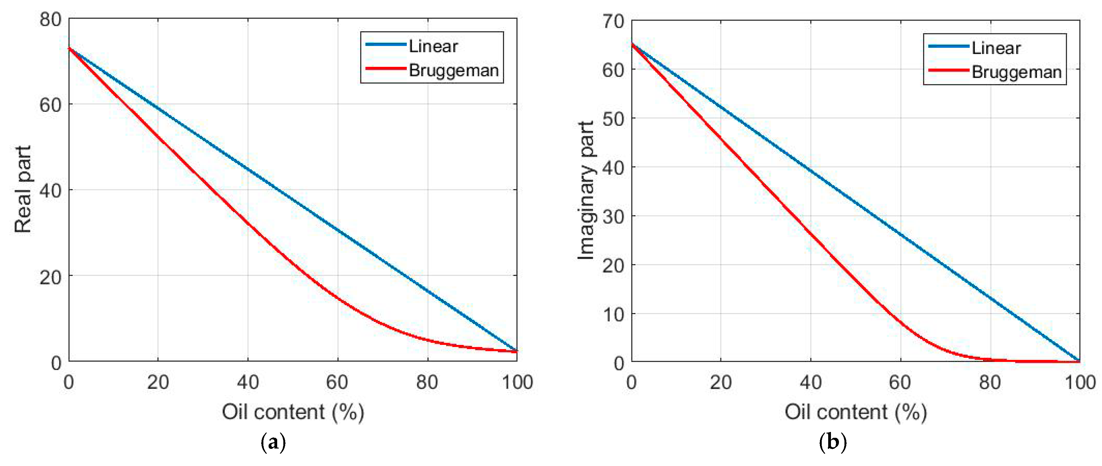
A linear mixing model is often employed [11,12] between mineral oil and seawater (5) to estimate the effective dielectric constant of an oil-in-water mixture, εeff. However, a more relevant approach from the Effective Medium Theory [28] advocates the use of the Bruggeman formula (6) to estimate the effective complex dielectric constant of such a mixture [21]:
where υ, ranging from 0 to 1, is the oil content (in volume) of the oil-water mixture, and εw and εoil are the relative dielectric constant of seawater and oil, respectively (Table 1). The real and imaginary parts of the effective dielectric constant of an oil-in-water emulsion are displayed in Figure 1 as a function of the oil content (in percentage) for both linear (blue curve) and Bruggeman’s model (red curve). One can observe a strong overestimation of both real and imaginary parts of the effective dielectric constant with the linear model compared to the Bruggeman formula. This overestimation is more pronounced at high concentration of oil (oil content~60–80%). In the following, the Bruggeman formula will be adopted to estimate the effective dielectric constant of an oil-in-water emulsion.
3. Airborne Campaign of Acquisition over Controlled Releases of Mineral Oil at Sea
3.1. NOFO’2015 Oil-on-Water Exercise
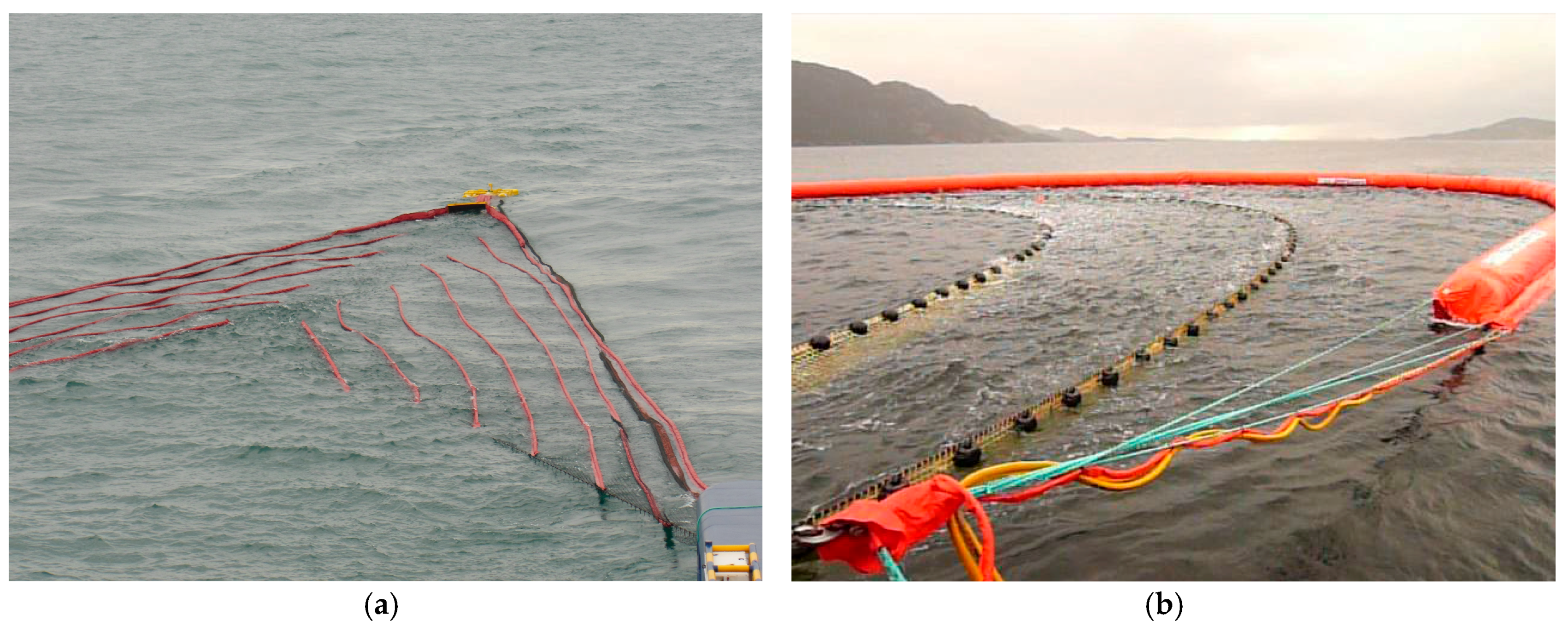
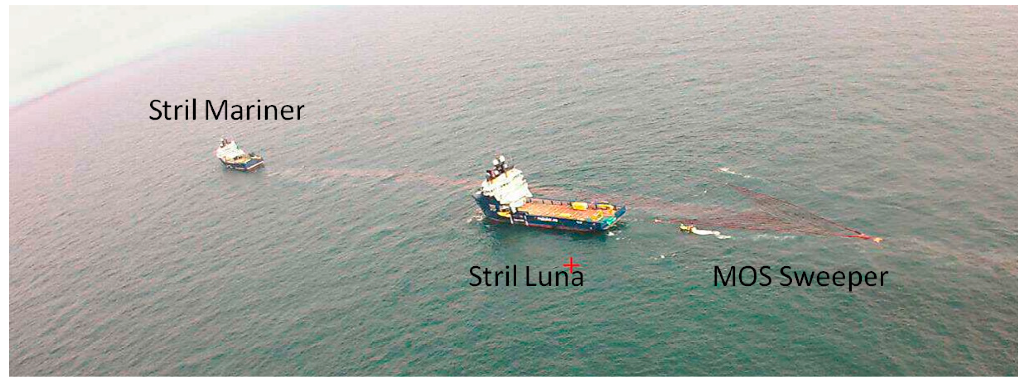
In June 2015, the NOFO (Norwegian Clean Seas Association for Operating Companies) has managed controlled releases of mineral oil at sea to test mechanical recovery systems. The oil spill cleanup exercise was carried out in the North Sea between the Norway and the United Kingdom within 10 Nautical Miles of position 59°59’N, 02°27’E. In the following we will focus on the 9 June exercises, during which the MOS Sweeper [29] and DESMI Boom [30] systems were tested at sea (Figure 2). For both experiments, hydrocarbons were released by a floating pump at the sea surface towed by a leading vessel (Stril Mariner) and recovered by a second vessel (Stril Luna), at only a few hundred meters. Figure 3 shows an illustration of the offshore spill area taken from a balloon during the MOS Sweeper experiment.
Trials with MOS Sweeper and DESMI Boom were conducted, respectively, in the morning (from 06:00 until 10:30 UTC) and in the afternoon (from 12:30 until 15:00 UTC) of June 9, using 45 m3 of mineral oil for MOS Sweeper and 35 m3 for DESMI Boom. The released product is an emulsion of mineral oil-in-water, with a water content of 60%. It consists of a mixture of seawater, Oseberg crude oil and a small addition of IFO 380 (Intermediate Fuel Oil or marine diesel oil, with viscosity of 380 mm2·s−1). The emulsion was prepared onshore by the NOFO several weeks before the exercises at sea. The stability and the exact constitution of the spilled product at the time of the exercise is therefore not precisely known.
Wind and waves information during the oil spill cleanup exercises was obtained from the Norwegian Meteorological Institute and is given in Table 2.
3.2. Airborne SAR Acquisitions
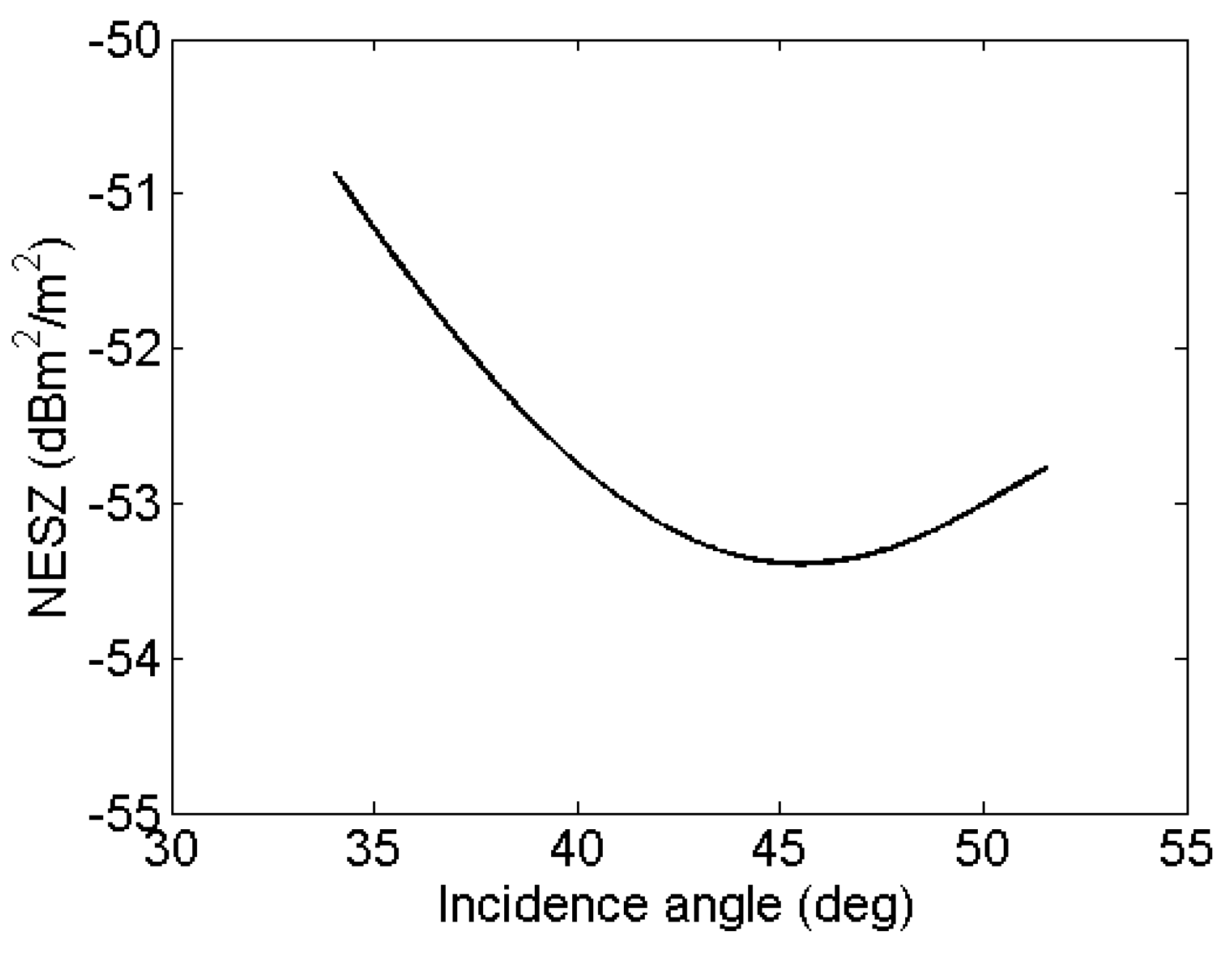
Polarimetric SAR (POLSAR) images were recorded during the oil-in-water exercise by SETHI, the airborne remote sensing system developed by ONERA [23]. POLSAR data in linear basis (HH, HV, VH, VV) were collected at L-band (EM frequency of 1.325 GHz) with a transmitted bandwidth equal to 150 MHz (range resolution of 1 m) and processed with an azimuth resolution of 1 m. The imaged area is 9.5 km in azimuth and 1.5 km in range, with incidence angles from 34° to 52°. SETHI is a high-resolution imaging radar characterized by a low instrument noise floor, see Figure 4 reproduced from [12], allowing a sufficiently high SNR over marine slick for efficient surface properties estimation.
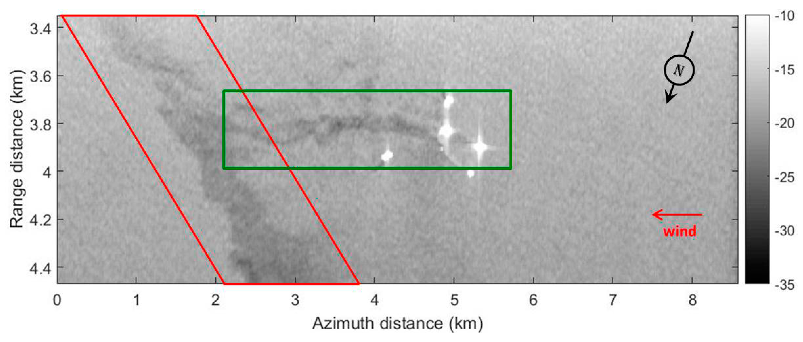
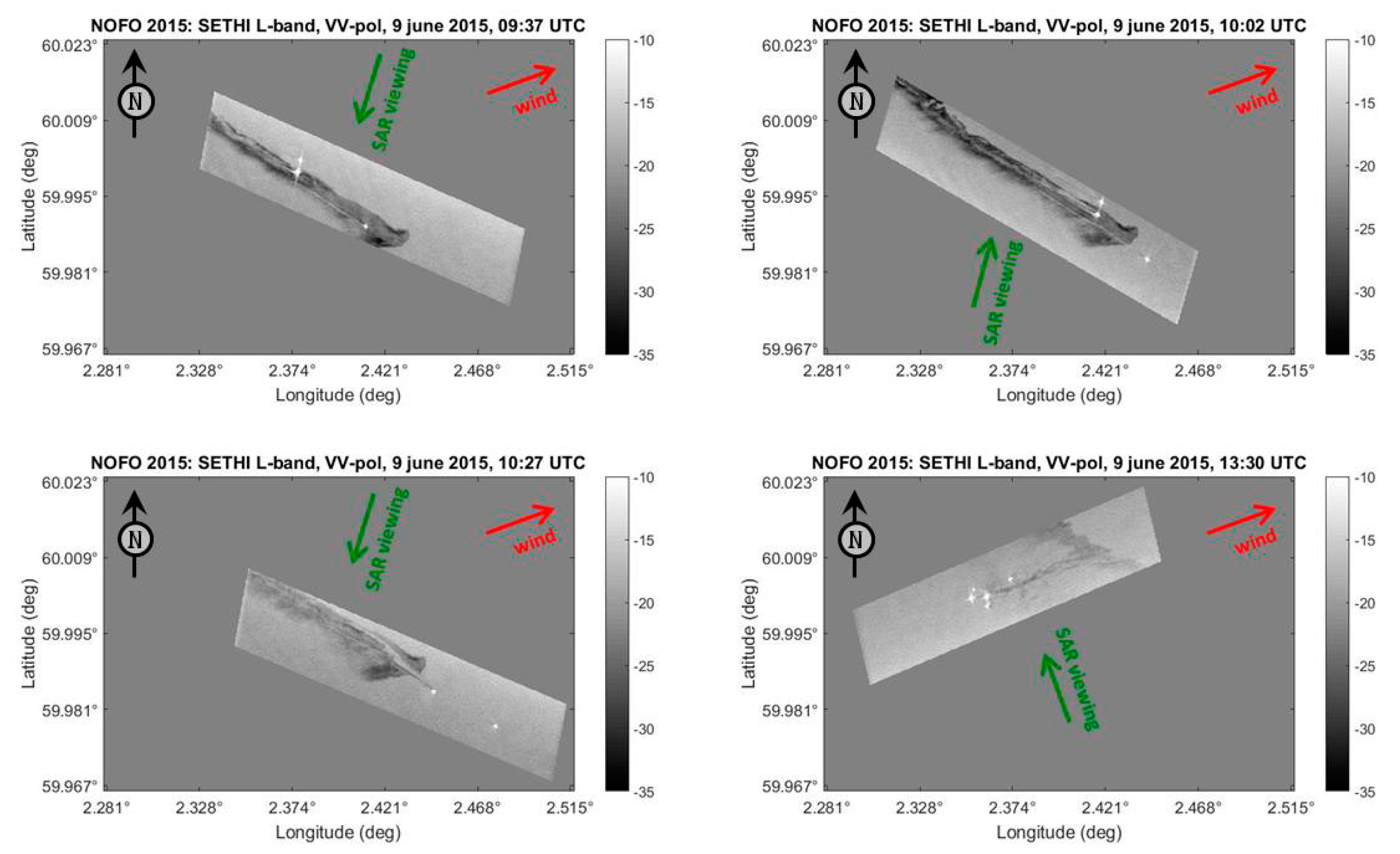
The SETHI remote sensing system flew over the oil spill area during the two cleanup exercises and collected SAR images throughout the 9 of June. In the following, four SAR scenes are investigated: three collected during the MOS Sweeper experiment at 09:37, 10:02 and 10:27 UTC and one at 13:30 UTC during the DESMI Boom exercise, cf. Table 3. The last one (run 4) was acquired 3 h after the last image of the MOS Sweeper exercise (run 3). Nevertheless, this image still contains part of the spill released during the morning experiment, MOS Sweeper, cf. Figure 5—red box. A 4-h temporal monitoring of this spill is then possible, between 09:37 UTC and 13:30 UTC.
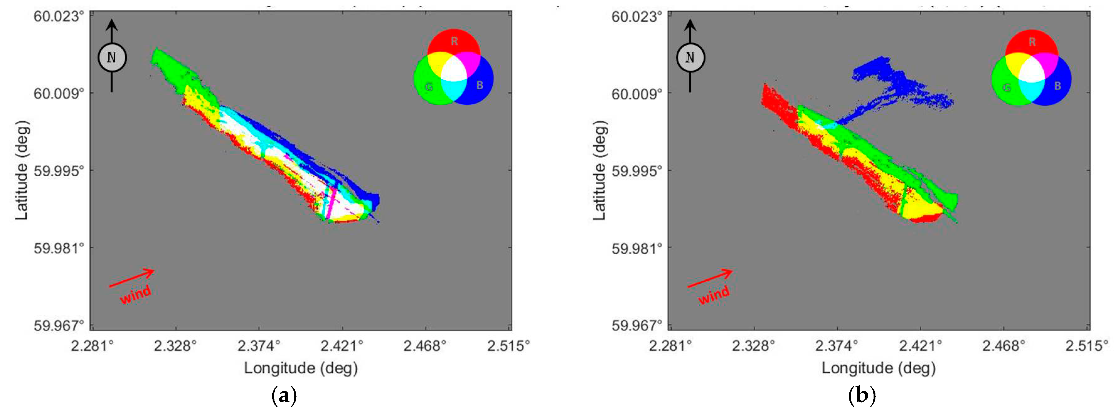
The four SAR scenes investigated in this paper have been projected from the slant range to the ground range geometry (Figure 6). The spilled area has been automatically detected using the polarization difference (in linear unit) between VV and HH channels [10,12,14,31] and the temporal evolution of the detected area is pictured on Figure 7 in a false color representation: drifting of the MOS Sweeper spill for one hour (from 09:37 to 10:27 UTC) in the morning of 9 June (Figure 7a) and drifting of the spill for four hours (from 09:37 to 13:30 UTC), Figure 7b. The spilled product during the MOS Sweeper exercise has drifted in the North-East direction, under the influence of wind (coming from 250°, cf. Table 2). The distance traveled by the spill between the first (09:37) and the last acquisition (13:30) is about 1.8 km in 4 h, which corresponds to a drift speed of about 0.125 m·s−1.
4. Estimation of Oil Concentration in an Oil-in-Water Slick Emulsion
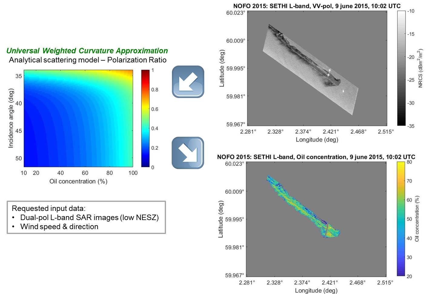
As discussed in Paragraph 2, the ratio between the two dual-co-polarized channels (3), at low frequency (e.g., L-band), is a useful quantity for measuring the concentration of oil within a marine slick [21]. The approach presented in this paper is based on the comparison between the polarization ratio measured by a radar operating at L-band and the values estimated by an analytical scattering model, namely the Universal Weighted Curvature Approximation (U-WCA), [22].
4.1. The Universal Weighted Curvature Approximation Scattering Model
With a remote sensing imaging radar collecting data at L-band, PR is only slightly impacted by changes in surface roughness but is mainly varying with the local incidence angle and the dielectric properties of the surface [11,12,21]. The proposed methodology for estimating the proportion of oil in an oil-in-water mixture is based on the comparison between the experimental value of PR with a scattering model, the Universal Weighted Curvature Approximation.
The U-WCA scattering model [22] belongs to the family of so-called “unified models” [32], such as the Two Scale Models (TSM) [6,33] or the Small-Slope Approximation [34], that is models which are able to cope with both large scales and small ripples at the sea surface. The U-WCA model leads to non-trivial roughness-dependent PR but has the considerable advantage of a simple formulation involving the nominal incidence angle only and requiring no facet decomposition. The expression of the co-polarized NRCS given by the U-WCA model is as follows
where Is is proportional to the classical Kirchhoff integral and Bpp and K are the Bragg and the Kirchhoff kernels [32], respectively.
In the Two Scale approach, ocean surfaces are usually modelled as a composition of slightly rough tilted facets, each of which has superimposed small-scale surface roughness that creates a Bragg scattering [6]. Small-scale roughness is randomly distributed on the scattering surface and responds to the strength of local wind, i.e., gravity-capillary waves. The tilt of the facet is caused by larger-scale waves on the ocean surface that changes the local orientation, or tilt, of the short waves [35]. The orientation of the facet changes the value of the local incidence angle of the EM wave interacting with the surface and therefore the levels of the backscattered signal and the polarization ratio. In general, a precise knowledge of the local incidence angle is not available; an approximation from SAR data can be obtained from an uncovered area close to the oil slick assuming homogeneous large-scale phenomena over the entire imaged area [11]. To overcome this strong limitation, the use of the U-WCA scattering model allows estimation of the polarization ratio without requiring the knowledge of the locale incidence angle [21,22], resulting from the local tilt of the facets composing the sea surface. In this paper, the polarization ratio measured by a radar sensor is compared to those estimated by the U-WCA model, the difference over slick covered area being linked to the modification of the effective dielectric constant compared to the surrounding clean sea surface.
PR values estimated with the U-WCA scattering model at 1.325 GHz are shown Figure 8. The simulation has been carried out in the upwind direction with the U-WCA scattering model using the classical Elfouhaily [36] sea surface directional spectrum. As expected, we observe strong variations of PR with the incidence angle but few variations with the sea surface roughness (Figure 8a). On the contrary, for a given value of incidence angle, PR values are strongly varying with the oil content into the oil-in-water mixture, especially for high oil concentration rates (Figure 8b). One can also note the strong difference between the Bragg theory (Figure 8a—black dotted line) and the U-WCA model (Figure 8a—colored full line). By construction, the U-WCA model, which is a weighted summation of Bragg and Kirchhoff kernels (see Equation (7)), produces higher PR than the pure Bragg model (recall that the Kirchhoff PR is one). This explains the discrepancy between the PR values computed using the Bragg theory (Equations (1)–(3)) and the U-WCA scattering model (Equation (3) with the HH and VV NRCS given by Equation (7)).
4.2. Comparison with L-Band Remote Sensing Data
A comparison between experimental and theoretical values of the polarization ratio at L-band is of primary importance and is displayed in Figure 9 with environmental conditions given in Table 2. Experimental values over slick-free (Figure 9a—blue line) and slick-covered (Figure 9a—red line) are computed over a range transect of L-band SAR data collected by SETHI during the NOFO’2015 experiment at 10:02 UTC (Table 3, run 2). We found a very good agreement between the PR values estimated by U-WCA (Figure 9a—black dotted line) and those measured by the SAR sensor over uncovered sea surface (Figure 9a—blue line). This confirms that at low EM frequency (e.g., L-band) the relative contribution of the non-polarized component with respect to the total power scattered from the ocean surface is negligible and hence that the scattering model can be used as a reference. The impact of mineral oil on the PR values is obvious, with a marked difference between histograms computed over free sea surface (Figure 9b—blue line) and covered area (Figure 9b—red line). This difference is due to the variation of the dielectric properties between the mineral oil slick and the surrounding clean sea surface. The quantitative estimation of the proportion of oil in an oil-in-water emulsion is made possible by comparing the PR measured by the remote sensing SAR data at L-band and the values estimated by the U-WCA scattering model, using a previously calculated data sheet (Figure 10a) allowing quick oil concentration estimation to meet operational constraints. For a given value of incidence angle, the unicity of the estimate is ensured by the monotonic variation of PR with the oil concentration (Figure 10a).
The data sheet of PR values estimated at L-band with the Bragg theory is displayed in Figure 10b. Compared to the U-WCA reference map (Figure 10a), the use of the Bragg model results in a strong overestimation of the oil concentration of a marine slick: an incidence angle of 45° and an actual value of PR value of 0.3 lead to an oil concentration estimate of 65% and 77% using the U-WCA (Figure 10a) and the Bragg model (Figure 10b), respectively.
5. Quantifying the Concentration of Oil within a Marine Slick with Real Airborne SAR Data
The methodology described in Section 4 has been first applied to L-band SAR data collected by SETHI at 10:02 during the MOS Sweeper oil spill exercise (Table 3, run 2). A VV polarized image is displayed in Figure 11 together with the experimental PR and the estimated oil concentration maps. A detection mask has first been applied, based on the thresholding of the polarization difference [10,12,14,31]. The ranges of variation of PR values and oil concentrations have been reduced to 0.15–0.35 and 20–80%, respectively, to enhance the visualization.
On the PR map (Figure 11b), one can observe strong variations of the PR values in the range direction due to the incidence angle changes across the swath. The second-order variation is due to the modification of the dielectric properties of the surface related to the oil content within the oil-in-water mixture. The oil concentration is estimated by firstly, selecting, for each pixel, the closest value between the actual PR and those given by the U-WCA data sheet (Figure 10a) and then by finding the concentration rate corresponding to the modelled PR value. The result is displayed in Figure 11c. The mean value of oil content within the emulsion is equal to 52% and more than 80% of the pixels within the slick have a concentration between 40 and 65%. Usually, the water content of marine oil slick lies between 50 and 75% [37], that is oil concentration between 50 and 25%. The values obtained in this experiment are slightly higher, which could be due to the relative short time lag between the release of oil by NOFO at sea and the scene acquisition by the radar sensor.
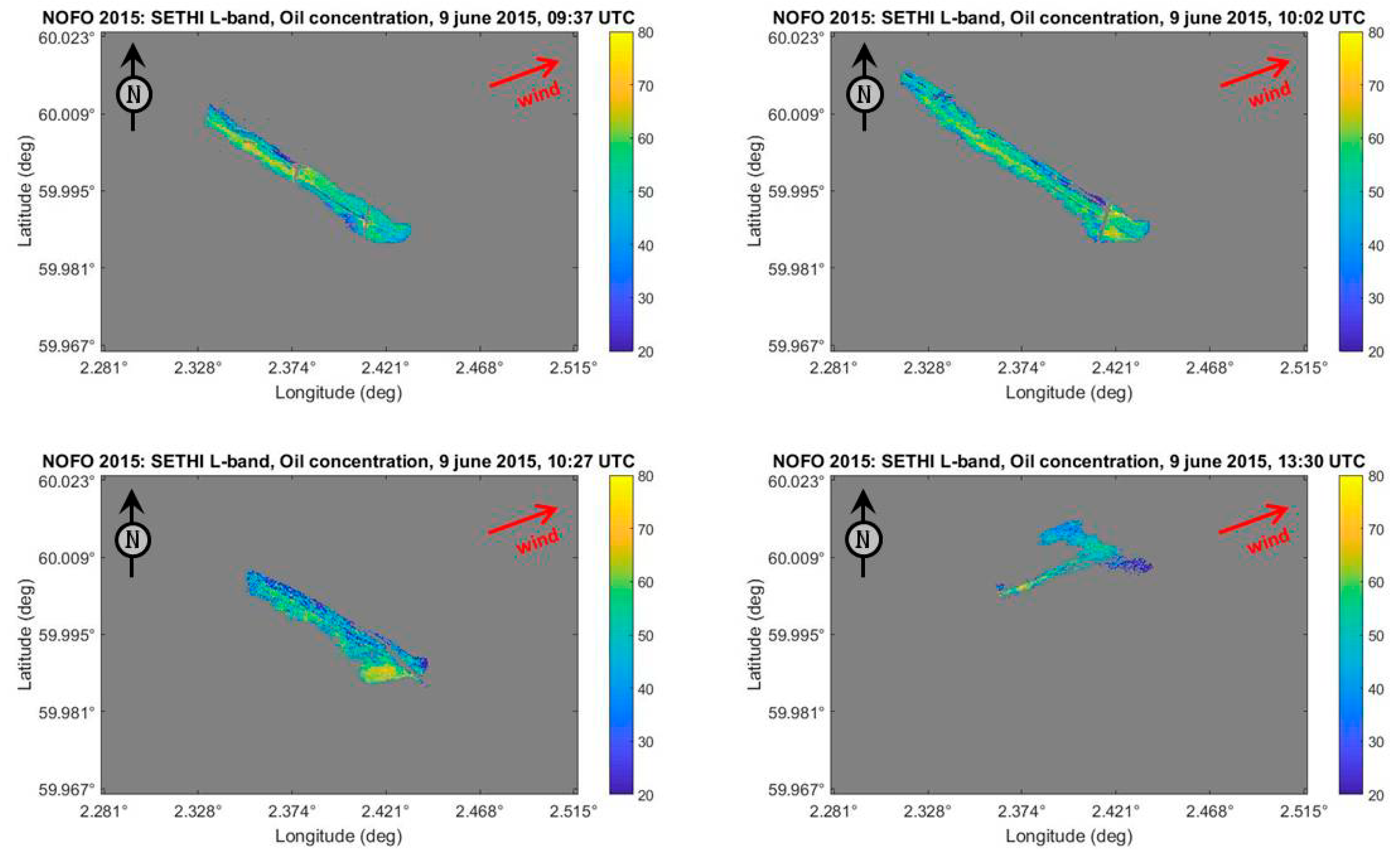
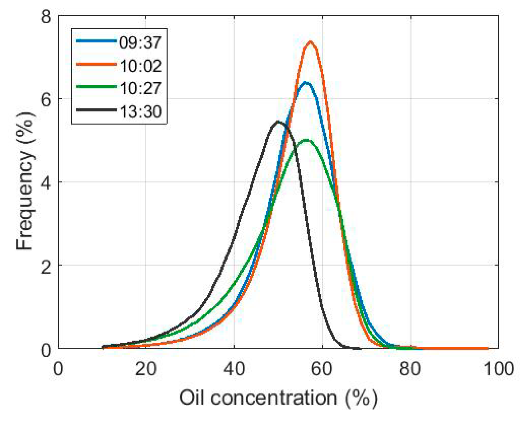
The same methodology has been applied to the other SAR scenes collected during the NOFO’2015 experiment and investigated in this paper (Table 3). All oil concentration maps have been projected in the ground geometry and are displayed in Figure 12 as well as the corresponding normalized histograms in Figure 13. The oil concentration underwent little change between 09:37 and 10:27 UTC (only 50 min) and no significant variation can be seen between the three histograms (Figure 13—blue, red and green curves). The average value of the oil concentration is 52%, 52% and 49% for the acquisitions of 09:37, 10:02 and 10:27 UTC, respectively. Compared to the first three histograms, the last histogram (acquisition at 13:30 UTC, 3-h later) is shifted to the lower values of oil content (Figure 13—black curve), with an average value of oil concentration of 43%. This decrease of oil concentration is due to weathering processes (wind, waves, evaporation …) whose impact is clearly highlighted on the oil concentration histograms.
6. Confidence in Oil Concentration Estimate
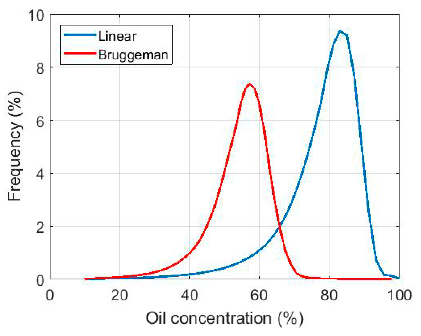
The quantification method proposed in this paper is based on the U-WCA scattering model and the Bruggeman formula for estimating the oil concentration from the effective dielectric constant of the oil-in-water mixture. Usually, a simple linear mixing between mineral oil and seawater is employed [11,12]. This important simplification leads to a significant error in the estimate of the oil concentration within an oil slick. The Figure 14 below shows two histograms of the oil concentration (run 2—10:02 UTC) obtained using a linear (blue curve) and the Bruggeman model (red curve). With a linear mixing, the histogram is shifted to the higher values of oil concentration, resulting in a strong overestimation of the average oil concentration (75% against 52%). These results show that the selection of the dielectric mixing model is a key aspect. The Bruggeman model has proven [28] to accurately reproduce the effective dielectric constant of an emulsion-type mixture and is highly recommended against the linear one when investigating the surface properties of marine slick from SAR imagery.
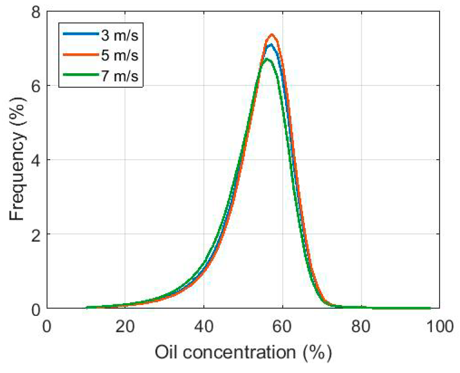
The second source of errors comes from the wind information which is one of the inputs of the U-WCA scattering model. This information usually comes from large-scale forecast models, which cannot describe local variations. According to the Norwegian Meteorological Institute, the wind speed (U10) was 5 m/s during SAR data acquisition at 10:02 UTC (run 2). The oil concentration has been estimated in a wind speed interval of +/− 2 m/s around the reported value. Histograms of oil concentration estimated from dual-pol SAR data collected at 10:02 UTC and for an input wind speed of 3, 5 and 7 m/s are shown in Figure 15. As discussed in Paragraph 4.1, at low EM frequency the polarization ratio has a weak dependence on surface roughness and therefore modelling with the U-WCA scattering model varies only slightly with wind speed. Hence, wind speed uncertainties induce little errors on the estimate of the oil content into the oil-in-water mixing. For the investigated SAR data collected at 10:02 UTC, the mean oil concentration is estimated to be 51.9%, 52.4% and 50.8% for a wind speed of 3, 5 and 7 m/s, respectively.
Since the remote sensing dataset explored in this study was not collected with validation data, no comparison between oil concentration estimate and in situ sampling within the spill areas can be performed. Even if the method reported in this paper is based on physical justifications, it cannot be formally validated. However, all the results presented herein are consistent with the expected behavior of an oil slick imaged area. First, the values of the oil concentration estimate are close to the concentration usually observed [37]. Then, we observe no trend of the estimation in the range direction, which suggests that the incidence angle variation across the swath as well been considered. Moreover, SAR data collected with a small time gap (09:37, 10:02 and 10:27 UTC) give similar oil content maps, despite the polluted area is differently positioned in the swath between the images, which ensures the robustness of the proposed methodology. Finally, the estimated maps covering the evolving spill over a 4-h period indicates a decrease of the average oil concentration, which can be attributed to weathering processes.
7. Conclusions
A methodology to estimate the proportion of oil within an oil-in-water marine slick mixture has been reported in this paper as well as its application to the temporal monitoring of the oil concentration. The key aspects of this study rely on three elements: the use of a rigorous surface scattering model to estimate the polarization ratio; the estimation of the volume fraction of oil from the Bruggemann formula; and the uniqueness of the dataset collected from controlled releases of mineral oil by an airborne SAR sensor operating at L-band, characterized by an instrument noise floor that is much lower than is currently available from spaceborne SARs.
At low frequency imaging radar (e.g., L-band), the relative contribution of non-resonant scattering with respect to the total backscattered energy from the ocean surface is negligible. For this reason, the polarization ratio measured by a radar sensor can be well approximated by a simple analytical scattering model such as U-WCA (see Figure 9a), which provides a non-trivial PR but depends only on the incidence angle of the incident radiation. Another advantage of using low frequency SAR images is that the ratio between the two co-polarized channels is only slightly dependent on the sea surface roughness but strongly affected by the dielectric properties of the imaged surface. This is not the case for higher frequency remote sensing radar, operating at C- or X-band. The volume fraction of oil within an oil-in-water mixture can then be retrieved from an Effective Medium Theory using the Bruggeman formula, by comparing the actual and the modelled polarization ratio at L-band.
The proposed methodology has been applied to an original set of L-band SAR scenes collected in June 2015 during an oil spill cleanup exercise carried out in the North Sea by the NOFO. Polarimetric SAR images have been acquired over controlled releases of mineral oil at sea by an airborne sensor characterized by a low instrument noise floor allowing a sufficiently high SNR over both slick-free and slick-covered areas for valid analysis of surface properties. Over freshly spilled mineral oil emulsion, the average oil concentration has been estimated to be above 50% with values ranging mainly from 40 to 65%. SAR data collected 4-h later permit to monitor the temporal behavior of the oil content and a decrease from around 50% to less than 45%, due to weathering processes, has been highlighted.
As shown in this paper, a combined utilization of an analytical scattering model and L-band SAR images collected with a sufficiently high SNR allows efficient estimation the concentration of oil within a marine oil slick (mixture between seawater and mineral oil). This estimation is shown to be robust to the uncertainties related to the sea state. Although no in situ measurements were collected with the remote sensing data, all the results presented herein are consistent with the expected behavior of an oil slick imaged area.
Author Contributions
S.A. conceived, design and performed the airborne experiments; S.A. analyzed the radar data; O.B., S.A. and C.-A.G. developed the methodology; S.A., O.B. and C.-A.G. wrote and revised the paper.
Funding
This work is funded by TOTAL (the French Oil and Gas Company) and ONERA (the French Aerospace Lab) under the NAOMI (New Advanced Observation Method Integration) project.
Acknowledgments
Research presented in this paper is part of the NAOMI (New Advanced Observation Method Integration) project funded by TOTAL (the French Oil and Gas Company) and ONERA (the French Aerospace Lab). The authors would like to thank all people involved in the NAOMI project, and especially Pierre-Yves Foucher from ONERA and Véronique Miegebielle and Dominique Dubucq from TOTAL for supporting this work. The authors are also very grateful to the NOFO (Norwegian Clean Seas Association for Operating Companies) for allowing them to participate in the Oil-on-Water exercise, which was carried out from the 8th to the 14th June 2015. Authors are very thankful for everyone involved in the experiment at sea and colleagues who participated to data processing.
Conflicts of Interest
The authors declare no conflict of interest.
References
- Fingas, M.; Brown, C. Review of oil spill remote sensing. Mar. Pollut. Bull. 2014, 83, 9–23. [Google Scholar] [CrossRef] [PubMed]
- Brekke, C.; Solberg, A. Oil spill detection by satellite remote sensing. Remote Sens. Environ. 2005, 95, 1–13. [Google Scholar] [CrossRef]
- Gade, M.; Alpers, W. Using ERS-2 SAR images for routine observation of marine pollution in European coastal waters. Sci. Total Environ. 1999, 237–238, 441–448. [Google Scholar] [CrossRef]
- Girard-Ardhuin, F.; Mercier, G.; Collard, F.; Garello, R. Operational oil-slick characterization by SAR imagery and synergistic data. IEEE J. Ocean. Eng. 2005, 30, 487–495. [Google Scholar] [CrossRef]
- Leifer, I.; Lehr, W.J.; Simecek-Beatty, D.; Bradley, E.; Clark, R.; Dennison, P.; Hu, Y.; Matheson, S.; Jones, C.E.; Holt, B.; et al. State of the art satellite and airborne marine oil spill remote sensing: Application to the BP Deepwater Horizon oil spill. Remote Sens. Environ. 2012, 124, 185–209. [Google Scholar] [CrossRef] [Green Version]
- Valenzuela, G.R. Theories for the interaction of electromagnetic and oceanic waves—A review. Bound.-Layer Meteorol. 1978, 13, 61–85. [Google Scholar] [CrossRef]
- Alpers, W.; Holt, B.; Zeng, K. Oil spill detection by imaging radars: Challenges and pitfalls. Remote Sens. Environ. 2017, 201, 133–147. [Google Scholar] [CrossRef]
- Wismann, V.; Gade, M.; Alpers, W.; Huhnerfuss, H. Radar signatures of marine mineral oil spills measured by an airborne multi-frequency radar. Int. J. Remote Sens. 1998, 19, 3607–3623. [Google Scholar] [CrossRef]
- Gade, M.; Alpers, W.; Hühnerfuss, H.; Masuko, H.; Kobayashi, T. Imaging of biogenic and anthropogenic ocean surface films by the multifrequency/multipolarization SIR-C/X-SAR. J. Geophys. Res. 1998, 103, 18851–18866. [Google Scholar] [CrossRef] [Green Version]
- Angelliaume, S.; Minchew, B.; Chataing, S.; Martineau, P.; Miegebielle, V. Multifrequency Radar Imagery and Characterization of Hazardous and Noxious Substances at Sea. IEEE Trans. Geosci. Remote Sens. 2017, 55, 3051–3066. [Google Scholar] [CrossRef]
- Minchew, B. Determining the mixing of oil and seawater using polarimetric synthetic aperture radar. Geophys. Res. Lett. 2012, 39, L16607. [Google Scholar] [CrossRef]
- Angelliaume, S.; Dubois-Fernandez, P.C.; Jones, C.E.; Holt, B.; Minchew, B.; Amri, E.; Miegebielle, V. SAR Imagery for Detecting Sea Surface Slicks: Performance Assessment of Polarization-Dependent Parameters. IEEE Trans. Geosci. Remote Sens. 2018, PP, 1–21. [Google Scholar] [CrossRef]
- Minchew, B.; Jones, C.E.; Holt, B. Polarimetric Analysis of Backscatter from the Deepwater Horizon Oil Spill Using L-Band Synthetic Aperture Radar. IEEE Trans. Geosci. Remote Sens. 2012, 50, 3812–3830. [Google Scholar] [CrossRef]
- Kudryavtsev, V.; Chapron, B.; Myasoedov, A.G.; Collard, F.; Johannessen, J.A. On Dual Co-Polarized SAR Measurements of the Ocean Surface. IEEE Geosci. Remote Sens. Lett. 2013, 10, 761–765. [Google Scholar] [CrossRef]
- Plant, W.J.; Irisov, V. A joint active/passive physical model of sea surface microwave signatures. J. Geophys. Res. Oceans 2017, 122, 3219–3239. [Google Scholar] [CrossRef]
- Makhoul, E.; López-Martínez, C.; Broquetas, A. Exploiting Polarimetric TerraSAR-X Data for Sea Clutter Characterization. IEEE Trans. Geosci. Remote Sens. 2016, 54, 358–372. [Google Scholar] [CrossRef]
- Ivonin, D.V.; Skrunes, S.; Brekke, C.; Ivanov, A.Y. Interpreting sea surface slicks on the basis of the normalized radar cross-section model using RADARSAT-2 copolarization dual-channel SAR images. Geophys. Res. Lett. 2016, 43, 2748–2757. [Google Scholar] [CrossRef] [Green Version]
- Quilfen, Y.; Chapron, B.; Bentamy, A.; Gourrion, J.; Elfouhaily, T.M.; Vandemark, D. Global ERS 1 and 2 and NSCAT observations: Upwind/crosswind and upwind/downwind measurements. J. Geophys. Res. Oceans 1999, 104, 11459–11469. [Google Scholar] [CrossRef] [Green Version]
- Horstmann, J.; Koch, W.; Lehner, S.; Tonboe, R. Wind retrieval over the ocean using synthetic aperture radar with C-band HH polarization. IEEE Trans. Geosci. Remote Sens. 2000, 38, 2122–2131. [Google Scholar] [CrossRef]
- Kudryavtsev, V.; Hauser, D.; Caudal, G.; Chapron, B. A semiempirical model of the normalized radar cross section of the sea surface, 2, Radar modulation transfer function. J. Geophys. Res. 2003, 108, 2156–2202. [Google Scholar] [CrossRef]
- Boisot, O.; Angelliaume, S.; Guerin, C.-A. Marine Oil Slicks Quantification from L-band dual-polarization SAR imagery. IEEE Trans. Geosci. Remote Sens. Submitted.
- Guerin, C.-A.; Soriano, G.; Chapron, B. The weighted curvature approximation in scattering from sea surfaces. Waves Random Complex Media 2010, 20, 364–384. [Google Scholar] [CrossRef]
- Angelliaume, S.; Ceamanos, X.; Viallefont-Robinet, F.; Baqué, R.; Déliot, P.; Miegebielle, V. Hyperspectral and Radar Airborne Imagery over Controlled Release of Oil at Sea. Sensors 2017, 17, 1772. [Google Scholar] [CrossRef] [PubMed]
- Zebker, H.A.; van Zyl, J.; Held, D.N. Imaging radar polarimetry from wave synthesis. J. Geophys. Res. 1987, 92, 683–701. [Google Scholar] [CrossRef]
- Meissner, T.; Wentz, W.J. The complex dielectric constant of pure and sea water from microwave satellite observations. IEEE Trans. Geosci. Remote Sens. 2004, 42, 1836–1849. [Google Scholar] [CrossRef] [Green Version]
- Folgerø, K. Bilinear calibration of coaxial transmission/reflection cells for permittivity measurement of low-loss liquids. Meas. Sci. Technol. 1996, 7, 1260–1269. [Google Scholar] [CrossRef]
- Friisø, T.; Schildberg, Y.; Rambeau, O.; Tjomsland, T.; Førdedal, H.; Sjøblom, J. Complex premittivity of crude oils and solutions of heavy crude oil fractions. J. Dispers. Sci. Technol. 1998, 19, 93–126. [Google Scholar] [CrossRef]
- Sihvola, A. Electromagnetic Mixing Formulas and Applications; IEE Electromagnetic Waves Series; Institution of Engineering and Technology: London, UK, 1999. [Google Scholar]
- MOS Sweeper. Available online: http://www.egersundgroup.no/oilspill/mos-sweeper (accessed on 20 April 2018).
- DESMI Boom. Available online: https://www.desmi.com/news-(3)/nofo-accelerates-spill-recovery-with-desmi-speed-sweep.aspx#1 (accessed on 20 April 2018).
- Hansen, M.W.; Kudryavtsev, V.; Chapron, B.; Brekke, C.; Johannessen, J.A. Wave Breaking in Slicks: Impacts on C-Band Quad-Polarized SAR Measurements. IEEE J. Sel. Top. Appl. Earth Obs. Remote Sens. 2016, 9, 4929–4940. [Google Scholar] [CrossRef]
- Elfouhaily, T.; Guérin, C.-A. A critical survey of approximate scattering wave theories from random rough surfaces. Waves Random Media 2004, 14, R1–R40. [Google Scholar] [CrossRef]
- Soriano, G.; Guérin, C.-A. A cutoff invariant two-scale model in electromagnetic scattering from sea surfaces. IEEE Geosci. Remote Sens. Lett. 2008, 5, 199–203. [Google Scholar] [CrossRef]
- Voronovich, A.G. Small-slope approximation in wave scattering from rough surfaces. J. Exp. Theor. Phys. 1985, 62, 65–70. [Google Scholar]
- Hasselmann, K.; Raney, R.K.; Plant, W.J.; Alpers, W.; Shuchman, R.A.; Lyzenga, D.R.; Rufenach, C.L.; Tucker, M.J. Theory of synthetic aperture radar ocean imaging: A MARSEN view. J. Geophys. Res. 1985, 90, 4659–4686. [Google Scholar] [CrossRef]
- Elfouhaily, T.; Chapron, B.; Katsaros, K.; Vandemark, D. A unified directional spectrum for long and short wind-driven waves. J. Geophys. Res. 1997, 102, 15781–15796. [Google Scholar] [CrossRef] [Green Version]
- Fingas, M.; Fieldhouse, B. Studies on water-in-oil products from crude oils and petroleum products. Mar. Pollut. Bull. 2012, 64, 272–283. [Google Scholar] [CrossRef] [PubMed]
Figure 1.
Effective dielectric constant of an oil-in-water emulsion plotted by increasing oil content using a linear model (blue) and the Bruggeman’s model (red): (a) real part; (b) imaginary part.
Figure 1.
Effective dielectric constant of an oil-in-water emulsion plotted by increasing oil content using a linear model (blue) and the Bruggeman’s model (red): (a) real part; (b) imaginary part.

Figure 2.
NOFO’2015 oil spill cleanup exercise: (a) MOS Sweeper and (b) DESMI Boom recovery systems tested on 9 June 2015 (photographs provided by NOFO).
Figure 2.
NOFO’2015 oil spill cleanup exercise: (a) MOS Sweeper and (b) DESMI Boom recovery systems tested on 9 June 2015 (photographs provided by NOFO).

Figure 3.
NOFO’2015—MOS Sweeper oil spill cleanup exercise (photograph provided by NOFO).

Figure 4.
SETHI instrument noise floor (NESZ) plotted by increasing incidence angle—reproduced from [12].
Figure 4.
SETHI instrument noise floor (NESZ) plotted by increasing incidence angle—reproduced from [12].

Figure 5.
SETHI L-band SAR data, VV-polarization, 13:30 UTC. Red box: MOS Sweeper spill. Green box: DESMI Boom spill—multi-look 21 × 21.
Figure 5.
SETHI L-band SAR data, VV-polarization, 13:30 UTC. Red box: MOS Sweeper spill. Green box: DESMI Boom spill—multi-look 21 × 21.

Figure 6.
SETHI L-band SAR data, VV-polarization, collected at 09:37 UTC (run 1—upper left panel), 10:02 UTC (run 2—upper right panel), 10:27 UTC (run 3—lower left panel) and 13:30 UTC (run 4—lower right panel)—multi-look 21 × 21—ground geometry.
Figure 6.
SETHI L-band SAR data, VV-polarization, collected at 09:37 UTC (run 1—upper left panel), 10:02 UTC (run 2—upper right panel), 10:27 UTC (run 3—lower left panel) and 13:30 UTC (run 4—lower right panel)—multi-look 21 × 21—ground geometry.

Figure 7.
SETHI L-band SAR data, detection masks in false color representation—ground geometry. (a) (Red,Green,Blue) = (09:37,10:02,10:27); (b) (Red,Green,Blue) = (09:37,10:27,13:30).
Figure 7.
SETHI L-band SAR data, detection masks in false color representation—ground geometry. (a) (Red,Green,Blue) = (09:37,10:02,10:27); (b) (Red,Green,Blue) = (09:37,10:27,13:30).

Figure 8.
Bragg theory and U-WCA scattering model. Polarization Ratio (PR) as a function of the incidence angle (a) for various wind speeds and (b) for various oil contents using the Bruggeman formula to estimate the effective dielectric constant of an oil-in-water mixing with a wind speed of 5 m/s. Values of the dielectric constant are taken from Table 1.

Figure 9.
PR at L-band (a) estimated with the U-WCA scattering model (dotted black) and measured with experimental SAR data (SETHI NOFO’2015 10:02 UTC) across a range transect over a clean sea surface (blue) and a slick-covered surface (red); (b) Normalized histograms of experimental PR values measured at L-band (SETHI NOFO’2015 10:02 UTC) over clean sea (blue) and slick (red) surface with an incidence angle of 46°.

Figure 10.
Reference map of PR values at L-band estimated with (a) the U-WCA scattering model and (b) the Bragg theory.
Figure 10.
Reference map of PR values at L-band estimated with (a) the U-WCA scattering model and (b) the Bragg theory.

Figure 11.
SETHI NOFO’2015 10:02 UTC. (a) L-band VV-pol image; (b) polarization ratio [0.15 0.35]; (c) oil concentration map [20 80%]—multi-look 21 × 21.
Figure 11.
SETHI NOFO’2015 10:02 UTC. (a) L-band VV-pol image; (b) polarization ratio [0.15 0.35]; (c) oil concentration map [20 80%]—multi-look 21 × 21.

Figure 12.
SETHI NOFO’2015 oil concentration map [20 80%] corresponding to the SAR data collected at 09:37 UTC (run 1—upper left panel), 10:02 UTC (run 2—upper right panel), 10:27 UTC (run 3—lower left panel) and 13:30 UTC (run 4—lower right panel)—multi-look 21 × 21—ground geometry.
Figure 12.
SETHI NOFO’2015 oil concentration map [20 80%] corresponding to the SAR data collected at 09:37 UTC (run 1—upper left panel), 10:02 UTC (run 2—upper right panel), 10:27 UTC (run 3—lower left panel) and 13:30 UTC (run 4—lower right panel)—multi-look 21 × 21—ground geometry.

Figure 13.
Normalized histograms of oil concentration estimated within the mineral oil slick released during the MOS Sweeper exercise. Temporal measurements at 09:37 (blue), 10:02 (red), 10:27 (green) and 13:30 UTC (black).
Figure 13.
Normalized histograms of oil concentration estimated within the mineral oil slick released during the MOS Sweeper exercise. Temporal measurements at 09:37 (blue), 10:02 (red), 10:27 (green) and 13:30 UTC (black).

Figure 14.
Normalized histograms of oil concentration estimated within the mineral oil slick released during the MOS Sweeper exercise (10:02 UTC) using the linear mixing model (blue) and the Bruggeman formula (red).
Figure 14.
Normalized histograms of oil concentration estimated within the mineral oil slick released during the MOS Sweeper exercise (10:02 UTC) using the linear mixing model (blue) and the Bruggeman formula (red).

Figure 15.
Normalized histograms of oil concentration estimated within the mineral oil slick released during the MOS Sweeper exercise (10:02 UTC) for an input wind speed of 3 m/s (blue), 5 m/s (red) and 7 m/s (green).
Figure 15.
Normalized histograms of oil concentration estimated within the mineral oil slick released during the MOS Sweeper exercise (10:02 UTC) for an input wind speed of 3 m/s (blue), 5 m/s (red) and 7 m/s (green).


| Surface | L-band [1.3 GHz] | C-band [5.0 GHz] | X-band [10 GHz] |
|---|---|---|---|
| Seawater (15 °C 35 PSU) | 73.0 + 65.1i | 66.8 + 35.7i | 52.9 + 39.0i |
| Mineral oil | 2.3 + 0.01i | 2.3 + 0.01i | 2.3 + 0.01i |
Table 2.
Environmental Conditions during the experiments.
| Date | Time (UTC) | Experiment | Wind Speed at 10 m (m·s−1) | Wind Direction (from-deg) | Significant Wave Height (m) |
|---|---|---|---|---|---|
| 9 June 2015 | 06:00 | MOS Sweeper | 5 | 250 | 1 |
| 09:00 | 5 | 250 | 1 | ||
| 12:00 | DESMI Boom | 7 | 250 | 1 | |
| 15:00 | 7 | 250 | 1 |
Table 3.
Properties of the SETHI L-band POLSAR scenes investigated in this study.
| Date | Run Number | Time of Imaging (UTC) | Cleanup Exercise | Flight Heading (deg) |
|---|---|---|---|---|
| 9 June 2015 | 1 | 09:37 | MOS Sweeper | 105 |
| 2 | 10:02 | MOS Sweeper | 290 | |
| 3 | 10:27 | MOS Sweeper | 105 | |
| 4 | 13:30 | DESMI Boom | 250 |
© 2018 by the authors. Licensee MDPI, Basel, Switzerland. This article is an open access article distributed under the terms and conditions of the Creative Commons Attribution (CC BY) license (http://creativecommons.org/licenses/by/4.0/).
Share and Cite
MDPI and ACS Style
Angelliaume, S.; Boisot, O.; Guérin, C.-A. Dual-Polarized L-Band SAR Imagery for Temporal Monitoring of Marine Oil Slick Concentration. Remote Sens. 2018, 10, 1012. https://doi.org/10.3390/rs10071012
AMA Style
Angelliaume S, Boisot O, Guérin C-A. Dual-Polarized L-Band SAR Imagery for Temporal Monitoring of Marine Oil Slick Concentration. Remote Sensing. 2018; 10(7):1012. https://doi.org/10.3390/rs10071012
Chicago/Turabian StyleAngelliaume, Sébastien, Olivier Boisot, and Charles-Antoine Guérin. 2018. "Dual-Polarized L-Band SAR Imagery for Temporal Monitoring of Marine Oil Slick Concentration" Remote Sensing 10, no. 7: 1012. https://doi.org/10.3390/rs10071012
Note that from the first issue of 2016, this journal uses article numbers instead of page numbers. See further details here.