1. Introduction
The soil is an important global reservoir of soil organic carbon (SOC), which plays a key role in understanding the global carbon cycle [
1]. Moreover, SOC determines soil aeration and water infiltration, and is an important source of soil nutrients [
2]. Traditional soil surveys are fundamental and necessary in obtaining accurate soil information and constructing a reliable dataset [
3]. The limited number of soil samples and the sampling cost hinder the quality of digital soil mapping. Therefore, a suitable soil sampling plan should be designed for high-quality and efficient digital soil map.
High-quality soil datasets enable high-precision digital mapping of SOC, which is essential in understanding the spatiotemporal variations in SOC and testing performance for different soil models [
4,
5]. The quality of soil dataset was influenced by the sampling density for the invisible and variable of soil properties [
3]. The quality of soil dataset has positive relationship with the sampling density for more soil samples can reveal more information of the soil properties. Additionally, the dispersion degree and spatial characteristics of SOC can influence the quality of digital soil mapping [
6]. The complex spatial distribution of SOC needs more soil samples to draw the trend of SOC in detail. Thus, it is a challenging work to balance the quality of the soil dataset and the number of the soil samples, and the construction of a high-quality soil dataset by a low sampling density remains challenging. A soil sampling plan determines the geographical locations of soil samples and influences the parameters of geostatistical models for digital soil mapping [
7]. Thus, a suitable sampling density plays an important role in displaying the spatial distribution characteristics of soil properties.
Soil sampling mainly aims to characterize the nutrient status of a study region as accurately and inexpensively as possible [
8]. Many typical soil sampling methods, such as traditional (random and grid sampling and their derivative methods) and model-based sampling strategies, such as zone, topographic/geographic unit, remote-sensing and Latin hypercube sampling (LHS), have been provided [
9]. The traditional methods were designed by the spatial distribution characteristics of the soil samples in the study area based on the random or grid ways. These traditional methods can be widely applied in different fields. However, the spatial characteristics of SOC should be considered in random sampling. Similarly, it is hard to select a suitable sampling distance for grid sampling with few prior knowledge [
10]. Therefore, the spatial characteristics of SOC and more valuable auxiliary information should be considered to resolve the limitations of traditional sampling methods. The model-based sampling strategies not only consider the spatial characteristics of the soil samples, but also the auxiliary variables that influence pedogenesis. With the development of remote sensing technology, soil covariate factors, including vegetation maps, geology maps and their derivatives, can be used as auxiliary variables for the digital soil mapping [
11]. These datasets play important roles in influencing soil properties, and the representative variables can be chosen for model-based soil sampling to select the suitable geographical locations of soil samples [
12,
13]. In the research of Minasny and McBratney [
14], a digital elevation model, slope, compound topographic index, and normalized difference vegetation index as the ancillary data were used to design one optimal and efficient soil sampling plan by a conditioned Latin hypercube sampling method. Lin, et al. [
15] explored the representative sampling points by a cluster analysis of soil environmental co-variates and then formulated a sampling design method. These researchers introduced a feasible and reasonable sampling method by easily acquiring exhaustive secondary information. However, the relationships between soil properties and environmental factors are uncertain in large regions and inconspicuous in small or field-scale regions [
16,
17]. Consequently, environmental factors cannot offer accurate auxiliary information for the spatial unbiasedness of soil properties, especially in field or local regions [
18].
Airborne hyperspectral imaging technology, which has attracted research attention in the study of natural and artificial materials, can respond to the spectral reflectance and absorption characteristics of study objects on land surface [
19,
20]. Visible and near-infrared (VNIR) spectral absorption features created by the electronic transition of soil carbon atoms, and the vibrational stretching and bending of O–H, C–H or C=O functional groups are important factors for quantifying SOC [
21]. Laboratorial or field VNIR reflectance spectroscopy is a valuable technique used to predict SOC [
17,
22]. Hyperspectral sensors placed on fixed-wing aircraft or helicopters can perform spatially continuous mapping with high spatial resolution, and spectral reflectance can capture the valuable information of topsoil [
18]. Many studies have indicated the potential of airborne or satellite hyperspectral images in the prediction of topsoil SOC or other properties [
23,
24,
25,
26]. Ciampalini, et al. [
18] used the prototypal multisensor hyperspectral system produced by Galileo Avionica, which consists of two electro-optical heads in VNIR and short-wavelength infrared (SWIR) spectral range (from 400 nm to 24,500 nm, over 700 bands) to obtain the hyperspectral images. Their study showed the ability of airborne hyperspectral data from relatively inexpensive and efficient sensing methods for producing reliable and high-resolution maps of clay content. Franceschini, et al. [
27] used the ProSpecTIR V-S sensor (SpecTIR LLC), which consists of two imaging sensors (AISA Eagle–Hawk; Specim), to obtain two aerial hyperspectral images. Each image contains 357 spectral bands from 400 nm to 2500 nm with a spatial resolution of 1 m and a spectral resolution of 4.6 nm in VNIR and 5.3 nm in SWIR. Their results showed that most of the soil properties (clay, sand, cation-exchange capacity, etc.) can be predicted using the airborne hyperspectral remotely sensed data with an increased accuracy. Although the soil masking by vegetation is one important issue in predicting soil properties by hyperspectral images, the residual spectra unmixing and semi-blind source separation methods were developed to separate the soil and vegetation spectra. Bartholomeus, et al. [
28] put forward a residual spectral unmixing to resolve the problem when fields are partially covered with vegetation. Ouerghemmi, et al. [
29,
30] developed a blind source separation method to separate the soil and vegetation spectra and a double-extraction approach for clay content estimation over semi-vegetated surfaces. All of these studies showed the potential of the airborne hyperspectral images in predicting the topsoil properties. Meanwhile, the spatially continuous mapping of hyperspectral images enables continuous digital soil mapping. Thus, hyperspectral images can introduce important auxiliary information to reflect the status of SOC and formulate an optimal soil sampling approach, especially at farm or field study scale. Moreover, hyperspectral images can resolve the disadvantages of environmental factors.
This study aims to (i) explore the reliability of airborne hyperspectral images in mapping the SOC of topsoil (0–15 cm); (ii) assess the sensitivity of sampling density in the digital mapping of SOC based on three sampling methods (random, grid, and LHS); and (iii) design one suitable sampling method based on three new evaluation indices, namely, ratio of sampling efficiency to performance (RSEP), density of soil samples index (DSSI), and comprehensive evaluation index of prediction accuracy (CEPA).
2. Materials and Methods
2.1. Study Area
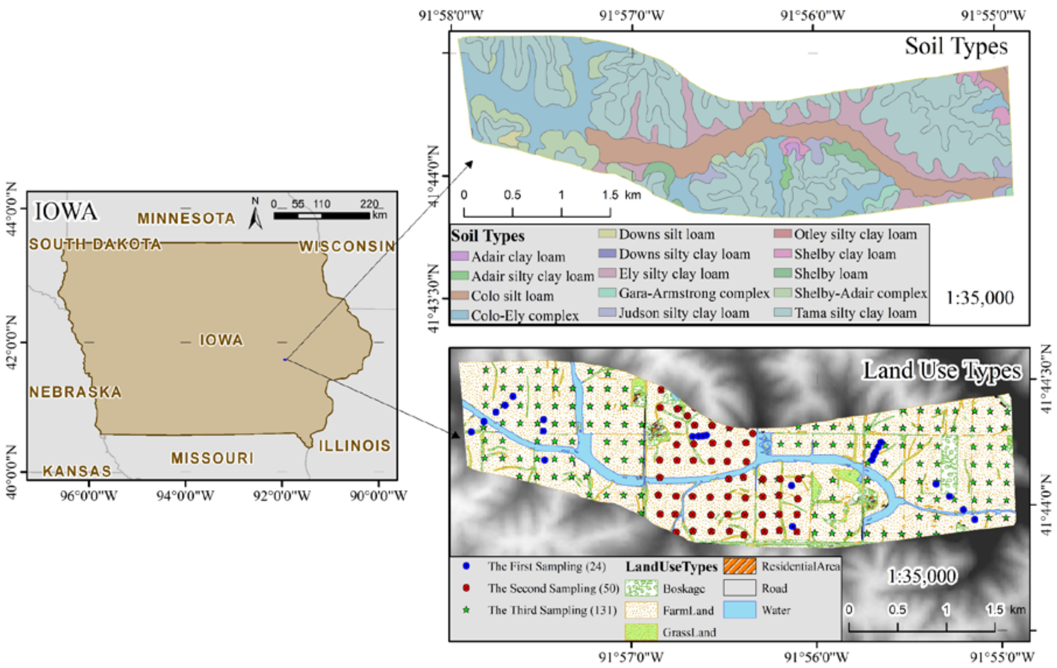
A farmland (approximately 385.45 ha) in southeast Iowa, United States, was selected as the study region (
Figure 1). Agriculture is a major economy component of Iowa, which is often called ‘the breadbasket of USA’, with 95% of its surface area devoted to cultivation of crops [
31]. This state has a humid continental climate because of its variable weather conditions. In addition, the climate in Iowa is cold and temperate with significant rainfall even in its driest month. The mean annual precipitation (including snowfall) is 903 mm, the mean snowfall is 104 mm, and the mean annual temperature is 9.8 °C which ranges from −11.6 °C in January to 18.3 °C in July. The geography of Iowa is generally not flat, and most of the state comprises rolling hills. The landform and topography is drift plain, with an elevation of 756–881 m and slope of 2°–23°. In the study area, the main land use type is farmland, and one river goes through the middle of the study area, and there are less vegetation and shrub. The main soil types in the study region are Typic Argiudolls, Cumulic Endoaquolls, Oxyaquic Argiudolls, Mollic Hapludalfs, and Aquic Hapludolls (
Figure 1), according to soil taxonomy class [
32]. The soils are formed by wind-blown, dominantly silt-sized particles known as loess. The topsoil and subsoil have a silty clay loam texture. The soil profile is dominated by silt-sized particles and generally less than 5% sand-sized particles. The topsoil layer has a granular structure that provides for water infiltration into the soil. The three-year crop rotations consisting of corn, soybeans, cereal rye, and red clover in the study area differ from the corn-soybean rotation commonly seen in Iowa, and the farmland is ploughed fallow by large machinery before seeding.
2.2. Soil Sample Collection and Analysis
Three soil sampling campaigns were conducted in May and October of 2015 and March of 2016. In May of 2015, 24 surface soil samples (0–20 cm) were collected in six places to obtain prior knowledge about the SOC in the study area. In October of 2015, 50 surface soil samples (0–20 cm) were collected using grid soil sampling with a sampling distance of 130 m. In March of 2016, 130 surface soil samples (0–20 cm) were collected using grid soil sampling with a sampling distance of 130 m. A total of 204 soil samples were used in this study. Soil samples were collected from farmlands that have been ploughed to avoid the influence of straw or weed. For each soil sample, five soil subsamples were collected from the four corners and the centre of a 1 m
2 sample square and thoroughly mixed for a representative sample. The soil samples were first air-dried in a laboratory at 20 °C to 25 °C for 14 days. The dried soil samples were gently crushed in a porcelain mortar to break up large aggregates, and sieved using a 2 mm stainless steel sieve. The soil samples were subjected to dry combustion using a CHNS combustion gas analyzer (Vario El Cube, Elementar, Germany) to determine SOC. Prior to analysis, the sample was acidified by HCl (4 mol/L) to remove carbonates. The combustion temperature ranged from 950 °C to 1200 °C, and the combustion time was approximately 10 min [
33]. The nonlinear correction curve was used to correct the analytical precision of the CHNS combustion gas analyzer, and the error was controlled to below 0.1% [
34].
2.3. Hyperspectral Images and Spectral Pre-Treatment
Aerial hyperspectral images (
Figure 2) were obtained on 19 November 2015 (10:00–14:00) using Headwall Micro-Hyperspec airborne sensors (SpecTIR LLC), which consisted of Micro-Hyperspec VNIR imaging spectrometers (A-Series) and Micro-Hyperspec NIR imaging spectrometers (X-Series). The aerial hyperspectral images were acquired after at least one week with no rain. The sun was shining brightly, and clouds were not apparent on the sky during image acquisition. The detail performance parameters of the Headwall Micro-Hyperspec airborne sensors were showed in
Table 1. A black landscaping material (50 m × 20 m), a light brown canvas (50 m × 20 m), and a white building material commonly known as Tyvek (50 m × 20 m) were used as reference objects to adjust the influence of the atmosphere, sunlight and other external factors. Radiation correction was applied using Hyperspec
® III with SpectralView™ (Copyright 2013, Headwall Photonics, Inc., Fitchburg, MA, USA). Raw data were converted into radiance using calibration files generated during radiometric and wavelength calibrations before and after sensor mobilization. Spectral reflectance was converted from spectral radiance on the basis of the empirical line correction in ENVI/IDL (Version 5.1, Esri Inc., Redlands, CA, USA). A standard three-band (red, green, and blue) orthorectified digital aerial photograph with 1 m spatial resolution scanned in 2011 was used for geometric corrections, which were applied using ENVI/IDL.
Aside from radiometric and geometric corrections, such factors as multicollinearity, random noise, and multiple scattering effects were considered. The aerosol concentration, the ozone content, and the water vapor column contents influence the spectral transmission process. These extraneous factors influence the robustness and accuracy of calibration models [
35]. Thus, pre-processing was important in spectral modelling, and partial least squares regression (PLSR) was used to build a soil spectral model. The calibration dataset consisted of the measured SOC values and the corresponding hyperspectral reflectance. In this research, 204 soil samples, which were collected through three samplings, were used to fit the relationships between SOC and spectral reflectance for digital soil mapping. Leave-one-out cross-validation was used to evaluate the accuracy of PLSR and check the spectral outliers based on different pre-processing methods. The MATLAB
® (R2008a, MathWorks, Inc., Natick, MA, USA) toolbox functionality was used to conduct a robust principal component analysis to detect and eliminate outliers from the original datasets. The wavelengths from 380 nm to 430 nm, and from 950 nm to 1000 nm in A-Series suffered from noise, and the range from 1350 nm to 1420 nm in X-Series were significantly influenced by water. Therefore, these wavelengths were removed in the prediction of SOC. After multiple tests, the Savitzky-Golay (SG) smoothing with a moving window of 30 nm was used to smoothen the radiance curves. Subsequently, and the log
10 was used to transform the spectral radiance. Finally, standard normal variate (SNV) was used as an example of a scatter-corrective method to partially remove undesired scatter- or particle-sized information from the spectrum reflectance pattern. Thus, a combined processing method of SG, log
10 and SNV was used to the spectral pre-process of soil samples. The spectral reflectance was used as explanatory variable to construct soil spectral models by PLSR after pre-processing. The PLSR and the pre-processing methods were implemented using the PLS toolbox (Version 7.9.3, Eigenvector Research, Inc., Wenatchee, WA, USA) and operated in MATLAB
®.
2.4. Ordinary Kriging (OK)
Kriging is an advanced geostatistical procedure that can generate a continuous surface from sparse soil samples on the basis of their attributes [
36]. In this research, OK was selected as the geostatistical model for estimating the spatial distribution of SOC on the basis of soil samples.
Z(
Xi) is assumed to be a regionalized variable (namely, SOC) with a variogram
γ(
h), which is a function describing the spatial aggregation field or stochastic process
Z(
u). In this research, the exponential (Formula 1), Gaussian (Formula 2), spherical (Formula 3), and circular (Formula 4) methods were used as the semi-variance model, and a suitable variogram based on the leave-one-out cross-validation results was selected.
The exponential function was defined as:
The Gaussian function was defined as:
The spherical function was defined as:
The circular function was defined as:
In these equations, a, a, 3a and are the effective ranges for the spherical, circular, exponential and Gaussian functions, respectively. h is the spatial lag, C0 is the nugget and C is the partial sill. The spatial variation of the soil samples for these variograms was isotropic.
Traditional OK can provide unbiased estimates with minimum error. The function of OK was expressed as:
where
,
is the predicted value of variable
z at location
x0;
is the measured data;
refers to the weights associated with the measured values and
n is the number of predicted values within certain neighbor soil samples. The standard search neighborhood defined by the ellipse parameters was used for OK [
37]. The sector type comprised four sectors with 45° offset, and the maximum and minimum neighbors were 5 and 2, respectively. The OK was implemented using the Create Fishnet tool in ArcGIS (Version 10.4.1, Esri, Inc., Redlands, CA, USA).
2.5. PLSR and Partial Least Regression Kriging (PLRK)
PLSR, which is a well-known modelling technique often used in chemometric and quantitative spectral analyses, is based on a linear transition from a large number of original descriptors to a new variable space based on a small number of orthogonal factors [
38]. A two-step descriptor selection procedure was applied to achieve the best model quality. The first step involved the dimensionality reduction of the spectral reflectance from thousands of wavelengths into a few valuable components. The pre-processing method of the spectral reflectance played an important role in this step. The second step involved selecting the suitable number of components and then fitting the relationships between the components and SOC contents. The root mean square error (RMSE) and
R2 of the leave-one-out cross-validation model (RMSE
CV and
R2CV) were important evaluation indices in this step. Additional details about the PLSR algorithm can be obtained from the study of Martens [
39].
PLSRK is a combined model that considers the predicted values of SOC by PLSR and the spatial correlation of the predicted residuals by OK. Two steps can be used to describe the PLSRK workflow. Firstly, the predicted SOC contents are obtained by PLSR and the predicted residuals of the SOC are estimated by OK in different semi-variance functions. Secondly, the predicted SOC content of PLSRK is calculated as the sum of the predicted SOC of PLSR and the estimated residuals of OK at the same locations. Additional information about PLSRK can be found in Guo, et al. [
17].
2.6. Sampling Methods
In this research, the grid sampling method was implemented using the Create Fishnet tool in ArcGIS. The fixed sampling distances between the neighbor soil samples were 40, 60, 80, 100, 120, 140, 160, 180, 200, and 220 m. The numbers of soil samples were 2414, 1075, 606, 388, 266, 203, 150, 117, 99 and 79, with sampling densities of 6.26, 2.79, 1.57, 1.01, 0.69, 0.53, 0.39, 0.30, 0.26, and 0.20 ha−1, respectively. Random sampling was implemented using the Create Random Points tool in ArcGIS, and the numbers of soil samples were the same with those in the grid sampling plans.
LHS is a statistical method of generating a near-random sample of parameter values from a multi-dimensional distribution [
40]. In the context of statistical sampling, a square grid containing sample positions is a Latin square if and only if only one sample is present in each row and column. A Latin hypercube is the generalization of this concept to an arbitrary number of dimensions, where each sample is the only one in each axis-aligned hyperplane [
14]. The LHS soil sampling plan was implemented using MATLAB on the basis of the number of grid soil samples and the geographical range of the study region. In this study, only the coordinate information was considered in designing the LHS sampling plan, and the numbers of soil samples were 2414, 1075, 606, 388, 266, 203, 150, 117, 99, and 79, which were the same with those under the two other sampling methods, thereby maintaining data consistency.
2.7. Evaluation Indices
The RMSE and
R2 of the calibration (RMSE
C and
R2C), RMSE
CV,
R2CV, the mean squared deviation ration (MSDR), and the ratio of standard deviation to RMSE (RPD) were used as the evaluation indices [
41,
42,
43] as follows:
where
n is the sample number;
is the measured value for the soil sample;
is the predicted value;
is the mean measured value; MSDR is the average of the ratios of the squared errors (MSE) to the kriging variances (
) at the prediction points, and
S.D is the standard deviation of the measured SOC from the validation dataset. In general, a model that performs well has large
R2 and RPD, and a small RMSE, and the number of MSDR should be close to 1.
2.8. Sampling Indices
Two important variables influence the performance of a soil sampling method, namely, the sampling density and the quality of the sample dataset. Three new indices (DSSI, CEPA, and RSEP) were developed in this paper to quantify the performance of soil sampling method. DSSI was used to describe the sampling density. The predicted capability of OK was used to replace the quality of sample dataset. CEPA was used to check the predicted accuracy of OK. Finally, RSEP was used as a comprehensive index to consider the equilibrium points of DSSI and CEPA, and a suitable soil sampling plan based on different demands was selected based on these three indices.
DSSI was used to evaluate the sampling density in different soil sampling methods, and its function was defined as follows:
where
f is the sampling density,
is the average sampling density,
d is the standard deviation of the sampling density and
n is the number of potential soil sampling methods.
CEPA was used to evaluate the quality of the soil datasets and defined as follows:
where
w is the reciprocal of RPD of the prediction model,
is the mean value of the reciprocal of RPD,
is the standard deviation of the reciprocal of RPD and
n is the number of potential soil sampling methods.
RSEP was defined as follows:
RSEP is a combination index of DSSI and CEPA and can be used to evaluate the comprehensive performance of the soil sampling plan. When RSEP is close to 0, the sampling method can balance the relationship between the sampling density and the quality of the sample dataset. Thus, the suitable sampling density is when RSEP is close to 0.
2.9. Soil Sampling Workflow
This research aimed to estimate one accurate and continuous SOC map using hyperspectral remote-sensing images through PLSR and PLSRK and explore the sensitivity of the number of soil samples in digital soil mapping using a traditional geostatistical model (OK). Furthermore, a comprehensive index (RSEP) was applied to select a suitable sampling density for digital soil mapping. This process involved four steps (
Figure 3).
The hyperspectral images were obtained using the hyperspectral sensors on the helicopter, and the radiation correction of the images and the pre-processing of the spectral reflectance were executed using the PLS toolbox operated in MATLAB®. Additionally, 204 soil samples were collected from the study region to construct the relationships between the hyperspectral reflectance and SOC.
PLSR and PLSRK were used to build the SOC prediction models, and the best soil spectral model based on R2 was used to predict SOC map of bare soil. The SOC map was used as the original referential map in the succeeding research.
Random, LHS, and grid soil sampling were simulated with different sampling densities on the basis of the original estimated SOC map. A total of 30 soil sampling plans were simulated in this research. The evaluation dataset consisted of 200 random soil samples was extracted from the original estimated SOC map. The RMSE, R2, and RPD were used to explore the sensitivity of sampling densities and geographical locations to the accuracy of digital soil mapping. In addition, DSSI was used to evaluate the sampling density, CEPA was used to evaluate the prediction accuracy of the OK models, and RSEP was used to select a suitable soil sampling plan and an appropriate sampling density.
The optimal soil sampling plan was executed in the study region, and the differences between the SOC maps predicted using the hyperspectral images and OK were then compared.
3. Results
The spatial distribution of SOC was predicted by the hyperspectral images using PLSR and PLSRK models. The evaluation indices showed that PLSRK has better prediction result than PLSR. The SOC map predicted by PLSRK was used as the reference map to check the performance of different soil samples. Three traditional soil sampling methods (random, grid and Latin hypercube sampling) with 10 classes of sampling densities (6.26, 2.79, 1.57, 1.01, 0.69, 0.53, 0.39, 0.30, 0.26, and 0.20 ha−1) were designed, and the performance of these sampling methods were quantified by DSSI, CEPA and RSEP. Also, one suitable soil sampling method can be designed, and the field sampling result also can verify the feasibility of these sampling indices.
3.1. Estimation of Referential SOC Map by Hyperspectral Images
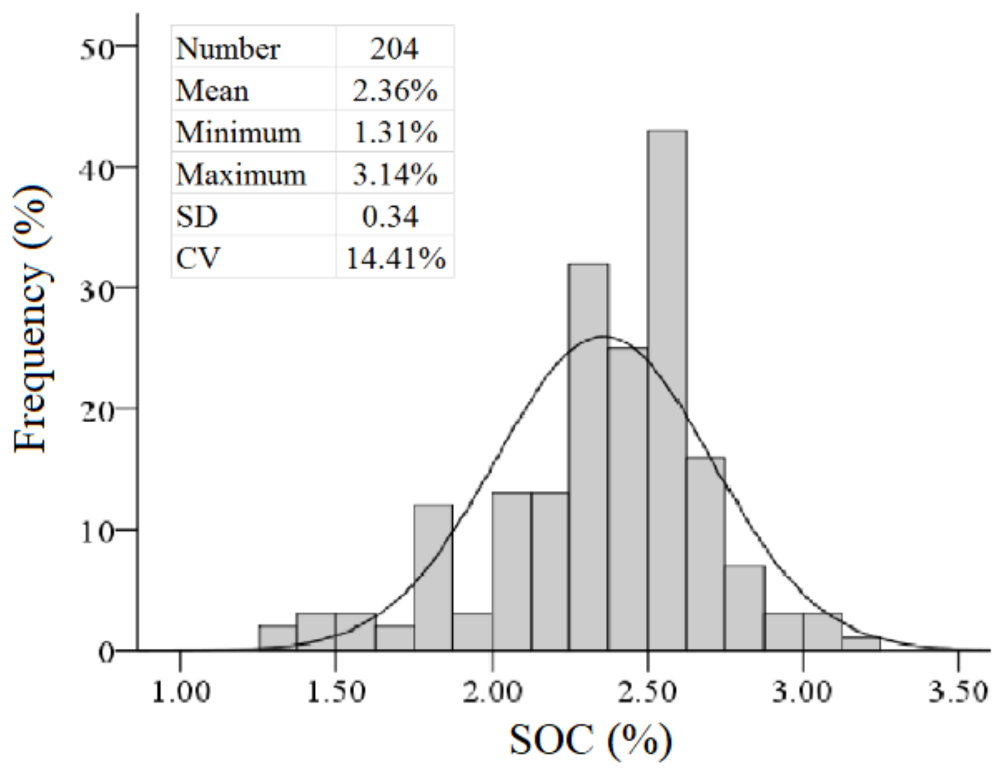
A total of 204 soil samples were analyzed using the histogram in
Figure 4, and the mean value of SOC was 2.36%, with values of 1.31% to 3.14%. The
S.D and coefficient of variation (CV) were used to evaluate the distributional characteristics of SOC content. The
S.D and CV were 0.34% and 14.41%, respectively. The histogram also showed the normal distribution of SOC. According to the study by Wilding [
44] in this region, these values indicated that SOC was a moderate variable. The main reason for this observation was that all the soil samples were collected from neighboring farmlands belonging to and managed by one family. Thus,
S.D and CV were excessively small, and the SOC content showed a minor difference.
The pre-processed hyperspectral reflectance was used to construct the prediction model for SOC using the PLSR model. The number of soil samples was 204, and the sampling density was approximately 0.529 ha
−1.
Figure 5a presents the predicted SOC map by PLSR. In this work, only the farmland with bare soil was selected as the study object. The other land use types were removed to decrease the influence of the land surface. The number of latent variables was five. The RMSE
C,
R2C, and RPD values of the calibration model were 0.17%, 0.77%, and 2.00%, respectively, whereas the RMSE
CV,
R2CV, and RPD values of the leave-one-out cross-validation model were 0.19%, 0.69, and 1.79, respectively. This result indicated the feasible prediction capability of the hyperspectral images in predicting SOC by PLSR. Thus, the soil hyperspectral model was used to estimate the spatial distribution of SOC in
Figure 5a. Several studies have shown that SOC is characteristic of a strong spatial autocorrelation [
45]. Furthermore, the Moran’s I value of SOC was 0.25 in the present study region. The Moran’s I was implemented in ArcGIS by the geostatistical tools. Thus, the regression–kriging model (PLSRK) was used to further improve prediction accuracy. The RMSE
CV,
R2CV, and RPD values of PLSRK were 0.17%, 0.75%, and 2.00%, respectively, whereas prediction accuracy was improved by 11.73% relative to PLSR, as indicated by RPD. Thus, the SOC map predicted by PLSRK was used as the reference SOC map to explore the sensitivity of the sampling density to the digital soil mapping (
Figure 5c). The SOC values of the farmland ranged from 0.55% to 3.91%. High and low SOC values were gathered from the northern and southern parts of the study region, respectively. The SOC residuals of PLSR ranged from −0.49% to 0.45%, according to the SOC residual map predicted by OK (
Figure 5b). The exponential model was used as the semi-variance one. The nugget was 0.026, the partial sill (C + C
0) was 0.045, and the major range was 1620.464 m. High positive and negative residuals were observed around and far from the river, respectively. The main reason for these values may be due to the soil moisture, which influenced the spectral reflectance of the field soil, which then affected the predicted results of the soil spectral models [
46]. These SOC maps could satisfactorily show the detailed spatial distribution characteristics of SOC in different geographical locations and offer important soil information for farmland management and sampling studies.
3.2. Simulation of Soil Sampling Plans
This study simulated three soil sampling plans (random, LHS and grid soil sampling) with 10 classes of sampling densities on the basis of SOC map predicted using the hyperspectral images (
Figure 5c).
Table 2 shows the parameters of the semi-variance functions by different soil sampling densities. These OK models selected the exponential function as the covariance function for different sampling plans due to the following reasons. (1) The exponential function was the optimal semi-variance function in the field example verification; (2) The same semi-variance function can remove the differences from different semi-variance functions.
Table 2 shows the detailed parameters of the different semi-variance functions. The sampling density was decided by the soil sample numbers and the study area. The nugget values means the un-estimated regionalized variable when less than the measure scale. The partial sill and sill showed the variation of variance which created by the spatial autocorrelation. Also, the nugget values were close to 0 in
Table 2, and this means the semi-variance functions can estimate the spatial variation of SOC. The C
0/(C + C
0) shows the degree of spatial variation, and most of these values were smaller than 50%, which showed that the spatial variation were mainly influenced by the spatial autocorrelation.
The evaluation dataset, including 200 random soil samples extracted from the referential SOC map (
Figure 5b), was used to evaluate the predicted accuracy of OK models and compare the performances of different soil sampling methods.
Figure 6 shows the corresponding evaluation indices. The double-factor analysis of the analysis of variance (ANOVA) was used to check the significance of these evaluation indices. The p values of RMSE, R
2, and RPD were 0.028, 0.008, and 0.042, respectively. All values were less than 0.05. Thus, the three soil samples exhibited significant differences. The RMSE values decreased with the increase of sampling density, whereas the R
2 and RPD values increased. In the random, LHS and grid sampling methods, the smallest values of RMSE (0.129, 0.140, and 0.123) and the largest values of R
2 (0.812, 0.790, and 0.755) and RPD (2.272, 2.172, and 1.999) were calculated at the highest sampling density (5.132 ha
−1). The largest values of RMSE (0.258, 0.239, and 0.252) and the smallest values of R
2 (0.256, 0.175, and 0.279) and RPD (1.113, 1.087, and 1.171) were computed at the lowest sampling density (0.163 ha
−1) (
Figure 6a). Therefore, the sampling density was an important factor that influenced the quality of the soil dataset. The quality of the sample dataset in these three sampling plans was favorable when the sampling density was high. Moreover, the evaluation indices showed that the grid sampling method had the lowest RMSE and largest R
2 and RPD relative to other sampling methods at the same sampling density. Therefore, the prediction accuracy of the grid sampling method was superior to that of the other two methods. This difference was probably because the sampling locations of the random and LHS sampling were random and the completeness of the representative soil samples cannot be guaranteed. The sampling distance of the grid sampling was fixed, and the soil samples were evenly spread over the main study area, which aided the modelling of the semi-variance function. Thus, the grid soil sampling method was relatively more stable, and preferred than the random and LHS sampling when the sampling density was similar.
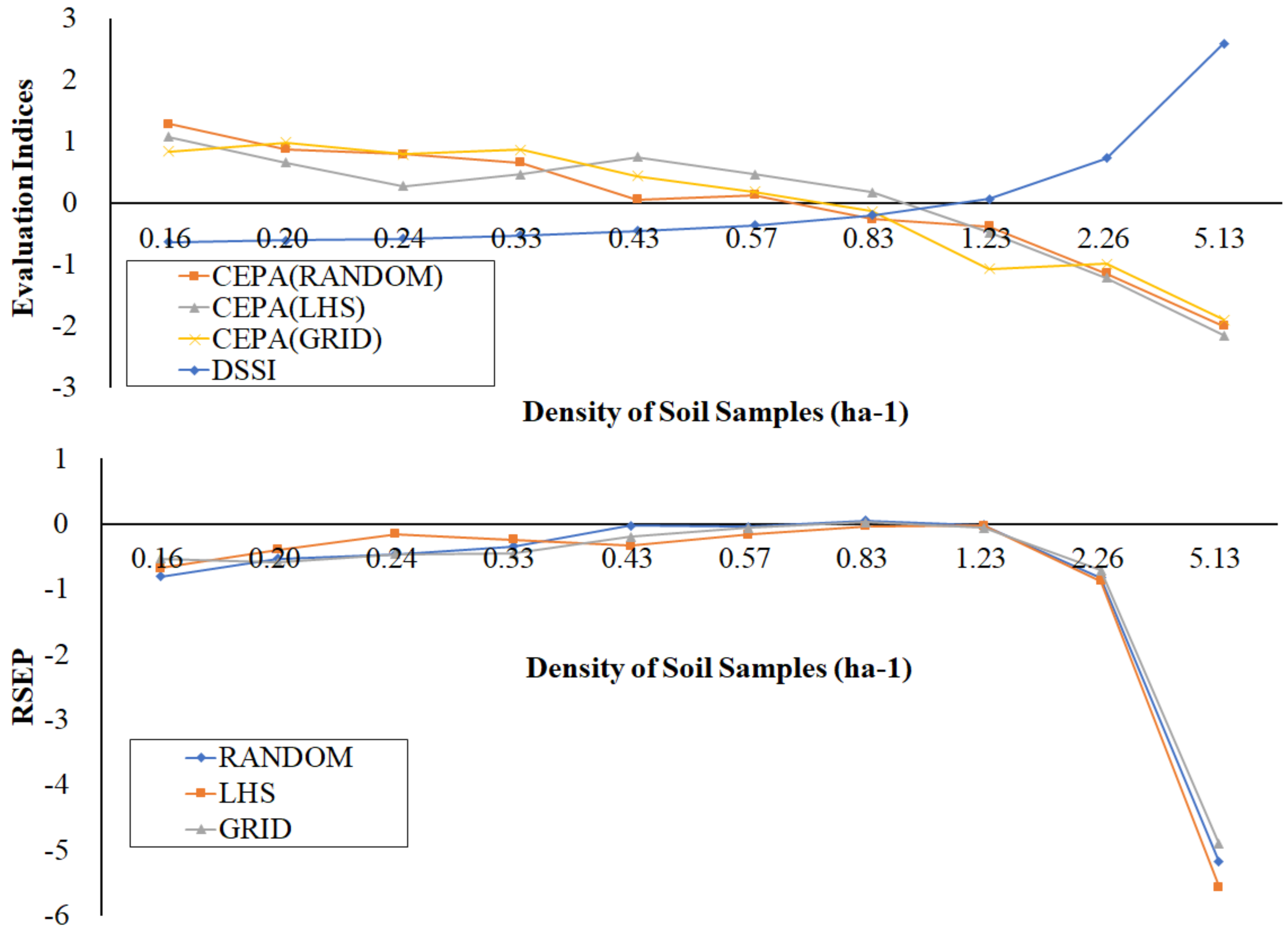
The evaluation indices DSSI, CEPA, and RSEP were calculated using the defined functions (10), (11) and (12).
Figure 7 shows the varying trends of DSSI, CEPA, and RSEP at different sampling densities. DSSI increased with the sampling density (The lower the DSSI, the less number of soil samples). DSSI had the largest value (2.589) at the sampling density of 5.13 ha
−1. The lowest value of DSSI was −0.634 and when the sampling density was 0.16 ha
−1. The CEPA values showed a decreasing trend with the increase of the sampling density. The larger the CEPA, the lower the prediction accuracy. CEPA had the smallest values at −2.001, −2.149, and −1.894 for random, LHS and grid sampling, respectively, at the sampling density of 5.13 ha
−1. Meanwhile, CEPA values were largest when the sampling density was 0.16 ha
−1. Moreover, most of the CEPA values of the grid soil sampling were lower than those of random and LHS sampling methods under the same sampling density. This result further indicated that the grid soil sampling method performed better than the other two methods. RSEP was a combination index of DSSI and CEPA. For random, LHS and grid sampling methods, RSEP showed an increasing trend at sampling densities from 0.16 ha
−1 (−0.810, −0.680, and −0.531, respectively) to 0.83 ha
−1 (0.052, −0.034, and 0.027, respectively) and then a decreasing trend to 5.31 ha
−1 (−5.181, −5.564, and −4.903, respectively). When the sampling density was higher than 0.83 ha
−1, the soil sampling plan required additional labor for the collection of soil samples. When the sampling density was lower than 0.83 ha
−1, the quality of the sample dataset was unsatisfactory. The performance of the soil sampling method was optimum when the RSEP value approached 0. Therefore, the suitable sampling density was from 0.43 to 1.23 ha
−1, which corresponded to the grid sampling distances of 140 to 80 m.
3.3. Comparison of Drawing Quality of SOC Maps
The sampling densities of 5.13, 0.57, and 0.16 ha
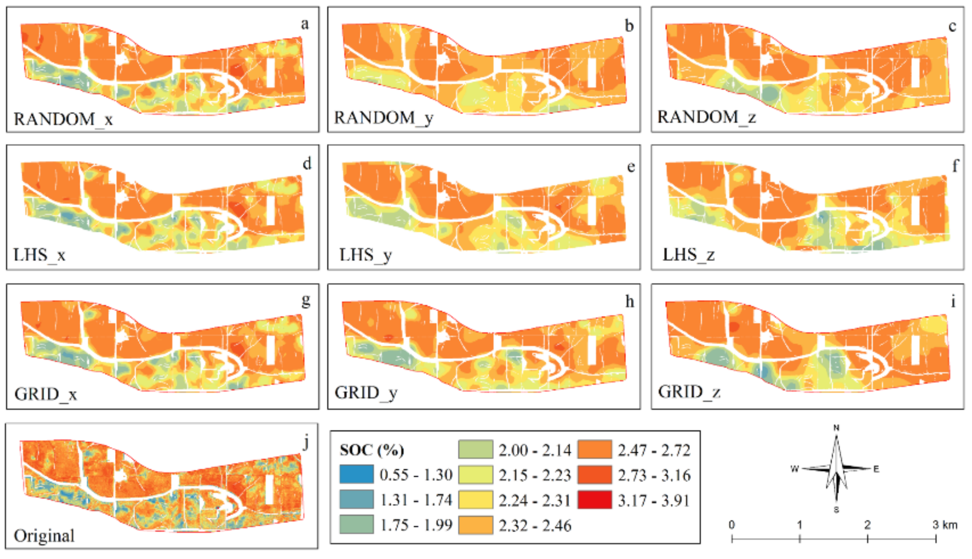
−1 were selected as study objects to show the differences of the estimated SOC maps in different sampling densities. Six SOC maps were predicted using the OK models based on random sampling, LHS and grid sampling with various sampling densities. The original SOC map, which was estimated by the hyperspectral images with a spatial resolution of 1 m, was used as the reference map (
Figure 8). Results showed that the quality of the predicted SOC map was favorable when the sampling density was high. When the sampling density was 5.13 ha
−1, the spatial distribution characteristics of the estimated SOC maps were similar to the original estimated SOC map. When the sampling density was 0.57 ha
−1 which was selected as the suitable sampling plan, detailed spatial characteristics of SOC were exhibited and the spatial trend of SOC became smooth and rough. When the sampling density was 0.16 ha
−1, little valuable soil information was described. Accurate soil maps could be predicted when the sampling density was high, but the field sampling work need more time and labor. However, at low sampling density, the spatial variability of SOC could not be showed in detail by a few soil samples. Meanwhile, when the sampling density was similar, differences of the soil maps using varying sampling methods could not be differentiated.
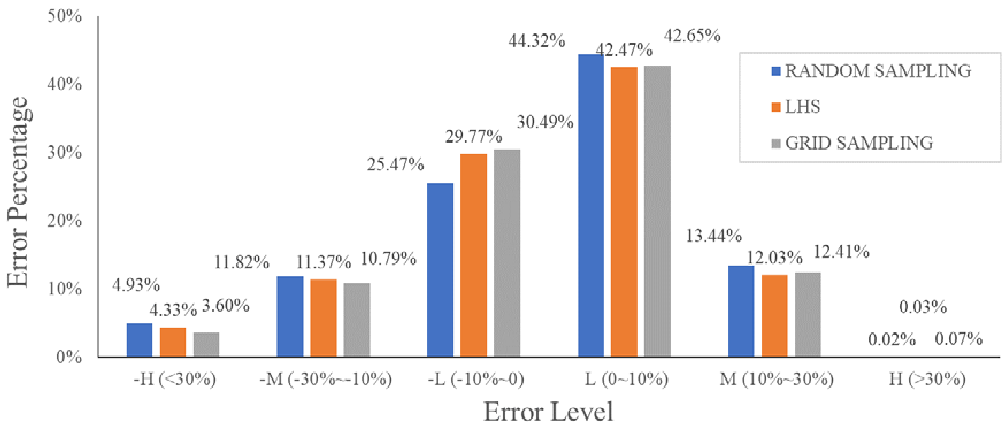
Figure 9 and
Figure 10 show the predicted error maps and histogram of the error values. These data further quantified the differences between the predicted SOC maps and the original referential SOC map. The error values were calculated on the basis of these two-series SOC maps. The error levels were defined as the percentage of the error values to the original SOC values (
). Six levels were divided on the basis of the percentages as follows: negative high level (−H: <−30%), negative median level (−M: −30% to −10%), negative low level (−L: −10–0%), low level (L: 0–10%), median level (M: 10–30%), and high level (H: >30%). Large predicted error values appeared on the southwestern, middle, and northeastern parts of the study region (
Figure 9a). The main reason can be due to different soil types, the topographic features, and the land use types in these regions, which lead to the strong spatial heterogeneity of SOC, thus the spatial distribution characteristics of SOC cannot be accurately estimated by the geostatistical model. More −H and −M regions appeared on the southwestern parts (
Figure 9a,b) than those shown in
Figure 9c. Meanwhile, more H and M regions appeared on the central parts (
Figure 9a,b) than those shown in
Figure 9c. Results showed that random sampling and LHS could easily create large estimation errors relative to the grid sampling method. In addition, the grid sampling method could accurately show the total spatial distribution characteristics of SOC. In
Figure 10, the summed areas of the −L and L levels (69.79%, 72.24%, and 73.14%) of the three soil sampling methods occupied most of the study region. This finding showed that a sampling density of 0.57 ha
−1 was acceptable. In addition, the low-level area of grid sampling (73.14%) was larger than that of the random sampling (69.79%) and LHS (72.24%). The high-level area of grid sampling (3.67%) was smaller than that of the two other sampling methods (4.36% and 4.95%). These data showed that the performance of the grid sampling method was superior to that of the two other techniques. To further verify the feasibility and accuracy of the grid soil sampling plan, grid sampling method with a sampling distance of 130 m (approximately 180 soil samples with a sampling density of 0.467 ha
−1) was used to collect the soil samples in this study.
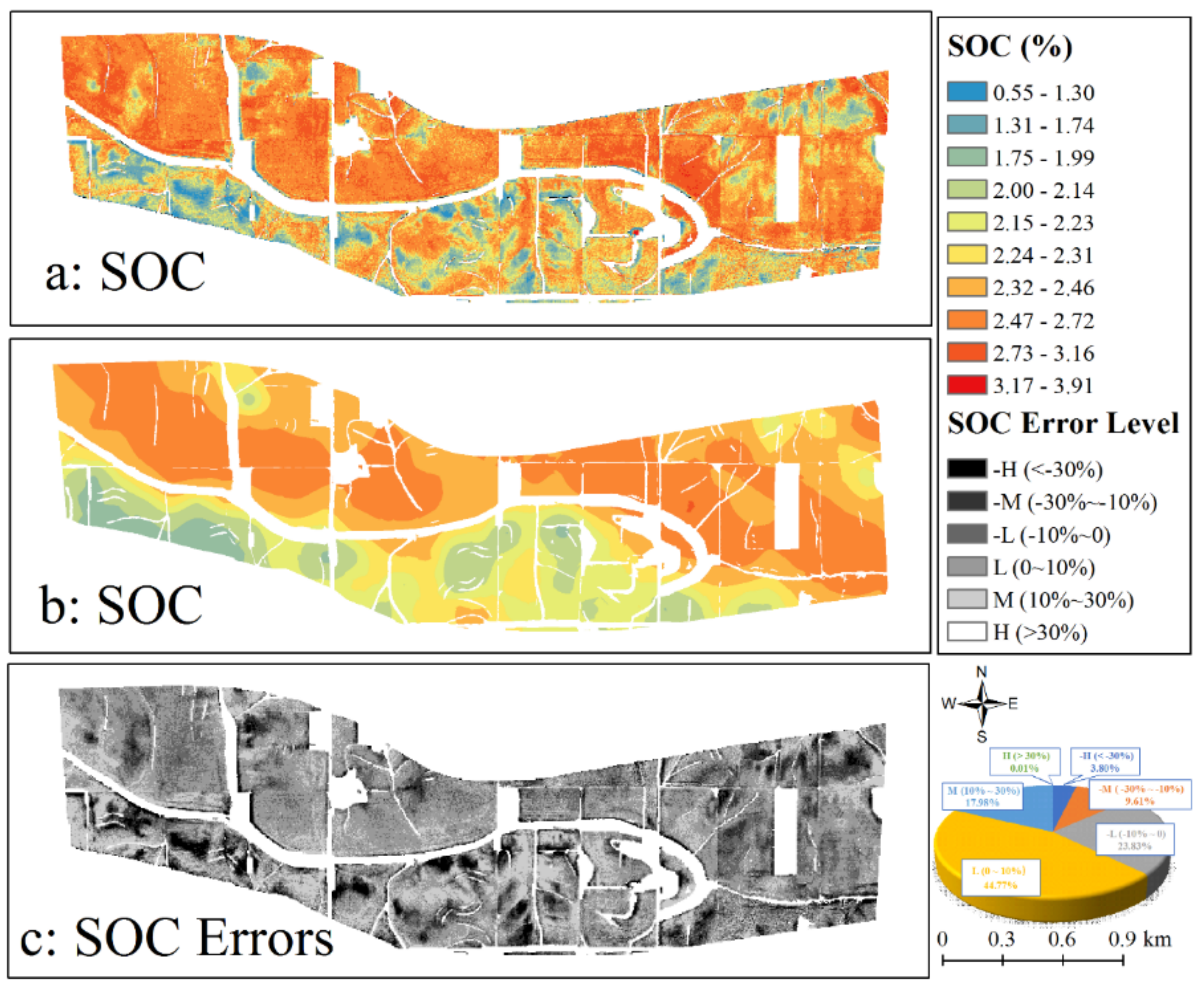
3.4. Evaluation and Application
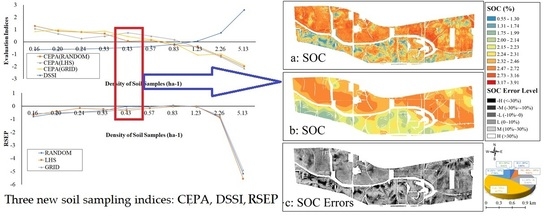
Grid soil sampling with a sampling distance of 130 m was selected as the soil sampling method. The original referential SOC map from
Figure 5a was used as the referential SOC map. Meanwhile, the SOC map predicted by the OK model based on the 180 grid samples was used to evaluate the performance of the grid sampling method, and the soil sampling density of the grid sampling method was 0.467 ha
−1. Various semi-variance functions were executed for the OK models.
Table 3 and
Figure 11 show the parameters. The RMSE and MSDR of the leave-one-out cross-validation were used to select the suitable semi-variance function, whereas the exponential model with RMSE of 0.3189% and MSDR of 0.823 was preferred.
Figure 12 presents the SOC error map between the original referential SOC map (
Figure 12a) and the predicted map (
Figure 12b) these two SOC maps. The figure illustrates the error levels using a pie chart. The overall distribution trend of SOC was similar in
Figure 12a,b, although the patches of SOC values in
Figure 12b were smoother than those in
Figure 12a. Areas with low (68.60%) and median (27.59%) error levels occupied more than half of the study region. High error levels were observed around the central river and regions with complicated soil types. The main reason can be due to the soil types in these regions were different. Different soil types were characterized by varying levels of soil moisture, and the soil moisture could influence the spectral reflectance of the hyperspectral images. This was why the high error levels always appeared around the middle river. In addition, the OK model could not accurately estimate the local spatial variations of SOC in the transition regions of different land use types. Overall, the 130 m grid sampling distance (with a soil sample density of 0.467 ha
−1) could be used to display the total spatial distribution of SOC in the study region. RSEP was a useful index for evaluating the performances of different soil sampling methods and can be used to design a feasible and suitable soil sampling plan.
5. Conclusions
This study estimated an original referential SOC map on the basis of measured SOC values from 204 field soil samples and hyperspectral images by PLSR and PLSRK. Three soil sampling methods (random, LHS and grid sampling) were computer-simulated on the basis of the referential SOC map. Each soil sampling plan included 10 classes of sampling densities (6.26, 2.79, 1.57, 1.01, 0.69, 0.53, 0.39, 0.30, 0.26, and 0.20 ha−1). The RMSE, R2 and RPD values were used to explore the sensitivity of sampling density in digital soil mapping, whereas RSEP, CEPA, and DSSI were used to select a suitable sampling density for describing the spatial distribution trend of SOC. Several interesting results were determined by synthetically comparing the performances of the three soil sampling methods with 10 classes of sampling densities.
(1) The hyperspectral images produced a relatively accurate SOC map with an R2CV of 0.69, RMSECV of 0.19%, and RPD of 1.79 by PLSR. The prediction accuracy of PLSRK was higher by approximately 11.73% than that of PLSR, which had an R2CV of 0.75, RMSECV of 0.17% and RPD of 2.00. The SOC map could display the trend of spatial distribution of SOC at a spatial resolution of 1 m. Thus, hyperspectral images could be used as a useful data source for the digital soil mapping of SOC.
(2) In the simulation of soil sampling plans, the R2, RMSE, and RPD values showed that sampling density had a positive relationship with the prediction accuracy of the estimated SOC map. The quality of soil sample dataset was favorable when the sampling density was high. Meanwhile, the performance of grid soil sampling was superior to that of random sampling and LHS at similar sampling density. Therefore, the grid soil sampling method was the first option for field sampling.
(3) Three new indices (DSSI, CEPA, and RSEP) were introduced to quantify the sampling density, prediction accuracy of digital soil mapping and comprehensive performance of the sampling plan. DSSI was negatively related to CEPA, and RSEP could balance the relationships among them. RSEP was nearly 0, which was a good balance point between DSSI and CEPA. RSEP showed that the suitable sampling density was from 0.43 ha−1 to 1.23 ha−1, which corresponded to grid sampling distances of 140 m to 80 m. In addition, the grid soil sampling plan with a sampling distance of 130 m (soil sample density was 0.467 ha−1) was executed in the study region. The prediction results verified the acceptability of this sampling plan. These data showed that RSEP was an effective index for selecting the suitable sampling density.
However, the disadvantages of the hyperspectral images, limitation of the field soil samples and other uncertainty factors generally influenced the performance of the soil sampling plan. Hence, additional studies and landscapes are necessary to evaluate the feasibility of the proposed sampling indices.


