Bidirectional Long Short-Term Memory Network for Vehicle Behavior Recognition


1
Key Laboratory of Spatial Information Smarting Sensing and Services, Shenzhen University, Shenzhen 518060, China
2
Computer Vision Research Institute, College of Computer Science and Software Engineering, Shenzhen University, Shenzhen 518060, China
3
College of Information Engineering, Shenzhen University, Shenzhen 518060, China
*
Author to whom correspondence should be addressed.
Remote Sens. 2018, 10(6), 887; https://doi.org/10.3390/rs10060887
Submission received: 13 May 2018
/
Revised: 27 May 2018
/
Accepted: 4 June 2018
/
Published: 6 June 2018
(This article belongs to the Special Issue Pattern Analysis and Recognition in Remote Sensing)
Abstract
:Vehicle behavior recognition is an attractive research field which is useful for many computer vision and intelligent traffic analysis tasks. This paper presents an all-in-one behavior recognition framework for moving vehicles based on the latest deep learning techniques. Unlike traditional traffic analysis methods which rely on low-resolution videos captured by road cameras, we capture 4K () traffic videos at a busy road intersection of a modern megacity by flying a unmanned aerial vehicle (UAV) during the rush hours. We then manually annotate locations and types of road vehicles. The proposed method consists of the following three steps: (1) vehicle detection and type recognition based on deep neural networks; (2) vehicle tracking by data association and vehicle trajectory modeling; (3) vehicle behavior recognition by nearest neighbor search and by bidirectional long short-term memory network, respectively. This paper also presents experimental results of the proposed framework in comparison with state-of-the-art approaches on the 4K testing traffic video, which demonstrated the effectiveness and superiority of the proposed method.
1. Introduction
Behavior recognition of moving objects is a hot research topic in multiple fields, especially for surveillance and safety management purposes. In this paper, we focus on city road traffic where the basic road element is the vehicle object.
Studying the behavior of on-road vehicles at road intersections is a vital issue for building intelligent traffic monitoring systems and self-driving techniques. For example, in order to ensure safe driving, drivers need to know if the vehicles in front are going straight through the intersection or are making left or right turns. However, due to the crossing of multiple roads, crashes generally occur at intersections [1]. In 2015, there were 5295 traffic crashes at four-way intersections with one or more pedestrian fatalities reported in the U.S. [2]. Hence, intelligent transportation systems need to actively monitor and understanding the road conditions and give warnings of potential crashes or the occurrence of the traffic congestion.
Conventional behavior recognition systems rely on thousands of detectors (e.g., cameras, induction loops, and radar sensors) deployed on fixed locations with small detecting ranges to help capture various road conditions throughout the network [3,4,5]. Such a system has exhibited many limitations in terms of range and effectiveness. For instance, if the information is required beyond the scope of these fixed detectors (i.e., blind regions), human labors are then frequently deployed to assess these particular road conditions [6]. In addition, many monitoring tasks need to temporally detect detailed traffic conditions such as sources and destinations of the traffic flow, regions of incidents, and queuing information at crossroads [7,8]. To achieve this, visual information of multiple fixed detectors needs to be aggregated in order to provide a relatively large view of the area of interest, which could introduce extra noisy information and overhead costs. Therefore, it is essential to develop a more effective approach for acquiring visual information for further processing.
To tackle these issues, previous works have attempted to exploit still satellite images for traffic monitoring [9,10,11]. Satellites can be used to observe wide areas, but they lack spatial resolution for specific ground locations. Additionally, data acquisition and processing are complicated and time-consuming, which hinders its application to real-time urban traffic monitoring tasks.
Thanks to the technological advances in electronics and remote sensing, Unmanned Aerial Vehicles (UAVs), initially invented for military purposes, are now widely available on the consumer market. Equipped with high-resolution video cameras, geo-positioning sensors, and a set of communications hardwares, UAVs are capable of capturing a wide range of road situations by hanging in the air or by traveling through the road network without restrictions [12,13,14,15]. Traffic videos captured by UAVs contain important information for traffic surveillance and management, and play an important role in multiple fields such as transportation engineering, density estimation, and disaster forecasting [16,17,18]. However, UAVs are not widely applied in the vehicle behavior recognition system due to specific challenges for detecting and tracking vehicles in the UAV’s images and videos.
On one hand, the equipped camera of a UAV may rotate and shift during the recoding process. On the other hand, compared with conventional monitoring systems, the UAV’s video contains not only the ordinary data such as the global view of the traffic flow, but also each vehicle’s own data regarding, for example, its moving trajectory, lane changing information, and its interaction with other vehicles [19,20]. Therefore, the UAV’s video needs to be recorded using a very high resolution and frame frequency so as to capture adequate ground details. This inevitably leads to a huge amount of UAV video data and poses challenges for vehicle detection and tracking algorithms [21].
To deeply understand city road vehicle behavior and overcome the challenges brought by real-world UAV video data, we developed a robust Deep Vehicle Behavior Recognition (DVBR) capable of recognizing different vehicle behaviors in high-resolution () videos. As a case study, we focus on vehicle behavior recognition at intersections.
The DVBR framework contains two main parts: the first consists in vehicle trajectory extraction. More concretely, we first trained a Retina object detector [22] to localize and recognize different vehicles (i.e., cars, buses, and trucks). Then we detected vehicles frame by frame on an input video, and developed a simple online tracking algorithm to associate detections across the whole video sequence. Based on the tracking results, we modeled and extracted vehicle trajectories from the original traffic video. To the best of our knowledge, this is the first framework which integrates deep neural networks and traditional algorithms for analyzing 4K () UAV road traffic videos.
The second part is vehicle behavior recognition. We approached this problem based on a nearest neighbor search and bidirectional long short-term memory, respectively. We conducted a comparative study in the experiments to demonstrate the effectiveness and superiority of proposed methods.
The rest of this paper is organized as follows. Section 2 briefly discusses work related to vehicle behavior recognition. Section 3 elaborates the Deep Vehicle Behavior Recognition Framework. Section 4 presents experiment settings, results, and discussion. Section 5 summarizes our work and discusses the path forward.
2. Related Work
Behavior recognition could be treated as the classification of time series data, for example, matching an unknown sequence to some types of learned behaviors [23]. In other words, behavior recognition in traffic monitoring describes the changes in type, location, or speed of a vehicle in the traffic video sequence (e.g., running, turning, stopping, etc.).
In general, the behavior recognition system contains a dictionary constructed using a set of pre-defined behaviors, and then finds matches in the dictionary by checking each new observation of the vehicle behavior, e.g., slow or fast motion, heading north or south [24]. Combined with the knowledge of traffic rules, these behaviors can be used for multiple applications, for instance, event recognition, which means generating a semantic interpretation of visual scenes (e.g., traffic flow analysis and vehicle counting), and abnormal event detection, such as illegally stopped vehicles, traffic congestion, crashes, red-light violation [25], and illegal lane changing [26].
Based on the vast amount of driving behaviors, there are two main approaches to understanding vehicle behaviors in road traffic scenes. The first one is vehicle trajectory analysis, and the other approach focuses on the explicit attributes of the vehicle itself, such as its size, velocity, and moving orientation.
2.1. Behavior Recognition with Trajectory
Many existing traffic monitoring systems are based on motion trajectory analysis. A motion trajectory is generated by tracking an object frame by frame in the video sequence and then linking its locations across the consecutive frames. In recent decades, various approaches to handle the analysis of the trajectory of moving objects based on city road traffic videos have been proposed. In [27], a self-organizing neural network is proposed to learn behavior patterns from the training trajectories, and activities of new vehicles are then predicted based on partially observed trajectories. In [28], the vehicle trajectories are modeled by tracking the feature points through the video sequences with a set of customized templates. Behavior recognition is then conducted to detect abnormal events: illegal lane changing or stopping, sudden speeding up or slowing down, etc. In [29], the turning behaviors of road vehicles is detected by computing the yaw rate using the observed trajectories. Based on the yaw rate and modified Kalman filtering, the behavior recognition system is capable of effectively identify the turning behavior. In [26], the lane changing information of target vehicles is modeled using the dynamic Bayesian network, and the evaluation is performed using the real-world traffic video data.
2.2. Behavior Recognition without Trajectory
Another way of recognizing behavior is to inspect non-trajectory information such as the size, velocity, location, moving orientation, or the flow of traffic objects [30]. The main objective is to, according to this information, detect abnormal events of a moving target if the values of these attributes exceed the pre-defined value ranges. In vision-based road traffic analysis, speed is estimated by converting the image pixel-based distances to the absolute distances by manual geo-location calibration. By extracting velocity data, the traffic monitoring system is able to quickly detect congestion, traffic accidents, or violation behaviors. For example, Huang et al. use the velocity, the moving direction, and the position of vehicles to detect vehicle activities including sudden breaking, lane changing, and retrograde driving [31]. Pucher et al. employ video and audio sensors to detect accidents such as static vehicles, wrong-way driving behaviors, and congestion on highways [32].
To summarize, much work has been done on road vehicle behavior recognition, but most published results rely on small camera networks, which means their cameras only capture a small range of the traffic scene, and they focus on specific vehicle tracking and activity analysis. Additionally, many approaches simply treat road vehicles as “moving pixels”, while the types of road vehicles are often ignored. For example, they cannot process a query such as “find all illegally stopped cars on Southwest Road” or “find all trucks queueing at red lights to cross the road”. In our work, we use the UAV to capture a large area of the road traffic. Our vehicle detection and tracking algorithms are able to recognize different types of vehicles and maintain these unique identities for tracking.
3. The Deep Vehicle Behavior Recognition Framework
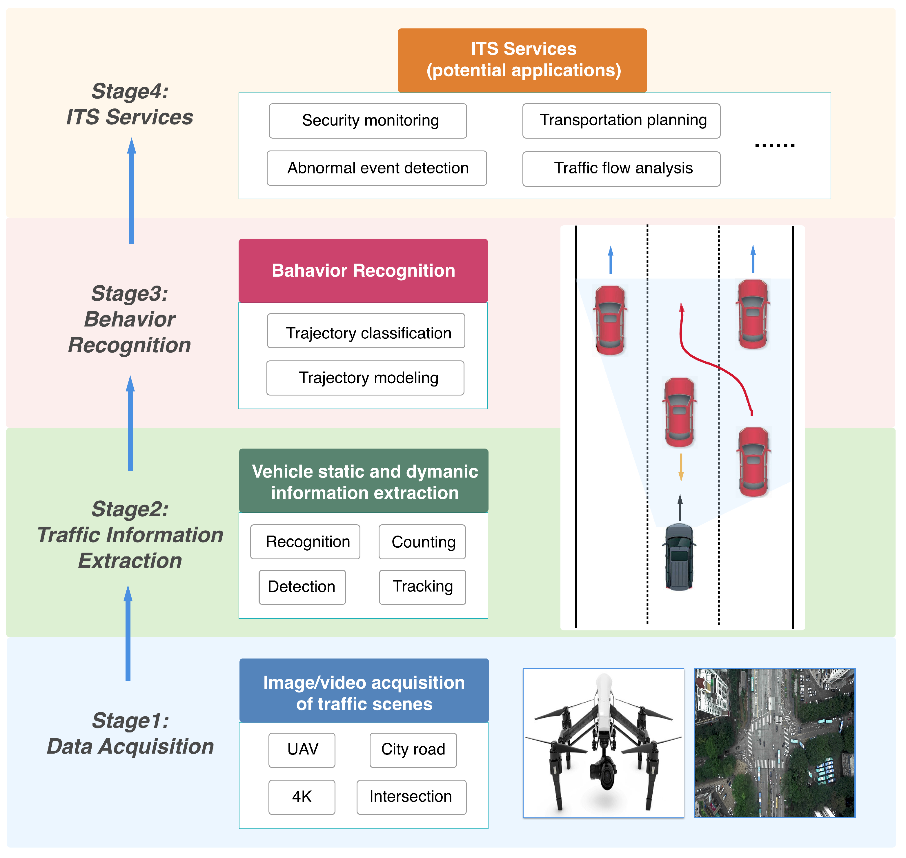
This section elaborates the DVBR framework. In the vehicle trajectory extraction part, we first detected road vehicles based on the Retina object detector [22] and then tracked vehicles by associated detections across whole video sequences. Next, we modeled and extracted the vehicle trajectories using the tracking results. In the behavior recognition part, we designed both semi-supervised and supervised approaches to classify vehicle trajectories in order to recognize their behaviors. Figure 1 illustrates an overview of our work and its relations to the intelligent transportation system (ITS).
3.1. Vehicle Trajectory Extraction
3.1.1. Vehicle Detection
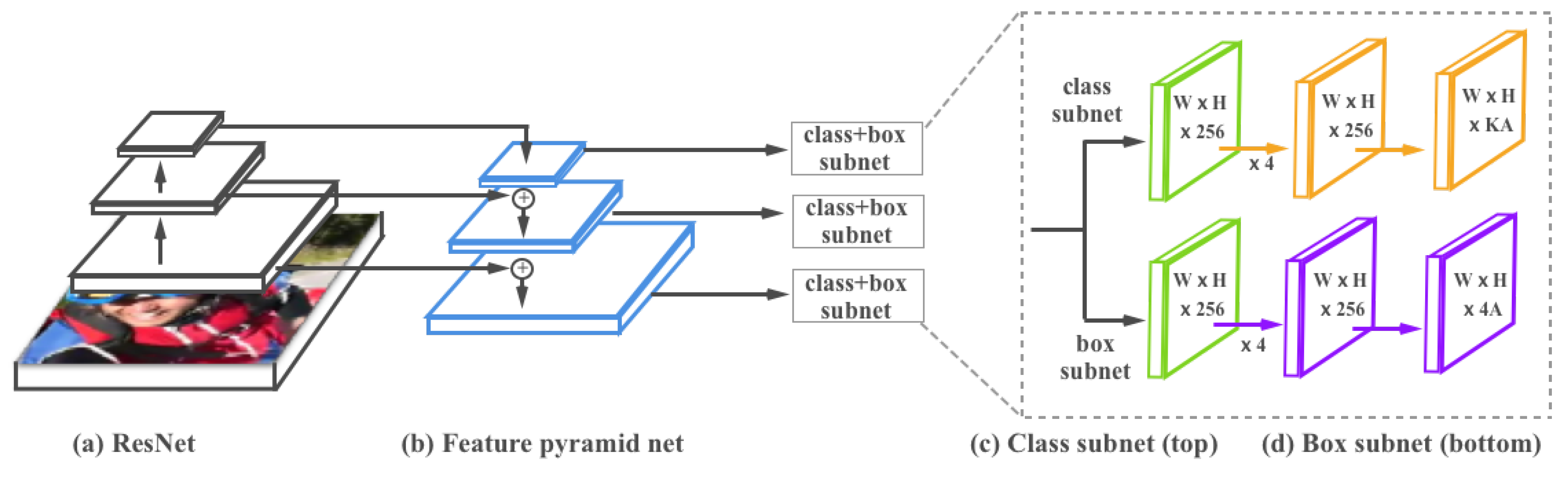
Network Architecture. We used RetinaNet [22] to detect vehicles in UAV videos. RetinaNet introduces the focal loss, which aims to address the one-stage object detection problem in which the foreground and background classes are imbalanced. It consists of a base network for multi-scale feature generation and two subnetworks for object detection (see Figure 2). The base network uses a Feature Pyramid Network (FPN) [33] on top of a feedforward ResNet [34] initially designed for image classification. The FPN can be seen as a standard convolutional network with top–bottom and lateral connections in order to build multi-scale (feature pyramid) feature maps for a single input image. Each layer of the pyramid is responsible for detecting objects at a specific scale.
The other two subnetworks are used for object detection. The first one is the classification subnet which predicts the probability of object existence at each spatial position for each bounding box location and C object categories. The second one is the box regression subnet which regresses the offset from each predicted bounding box to a nearby ground-truth object bounding box.
Training and Testing. We used the training images extracted from the training video to train the vehicle detector, and in the testing phase, a testing image was fed into the trained detector. Couples of predicted boxes with class confidences were generated as the initial output. For each unique vehicle, using a Non-Maximum Suppression algorithm [35], only a single prediction (bounding box and type) was reserved via thresholding.
One important issue in testing is that the original 4K () traffic video frames are too large for the network input. To solve this, we designed a region-based strategy by employing a sliding window to divide the original video frame into small patches with a size of . We allowed an overlap of 200 pixel horizontally and vertically between patches in order to capture complete vehicles. We then performed detections on each image patch and stitched them back together to the initial scale.
Allowing overlaps between these patches sometimes yielded complete detections, but this also increased the numbers of repeated detections (i.e., a single vehicle was detected multiple times in different patches). To solve this issue, in our experiment, we found repeated boxes by evaluating them: either their center distances were smaller than a threshold () or their intersection-over-union (IoU) scores were above a threshold (). IoU is a popular evaluation criterion in the field of object detection [36,37], and is used to measure the ratio of overlap between two bounding boxes. In our case, the IoU score of two predicted boxes and is
represents a complete match between two bounding boxes. After we obtained all repeated boxes on a single vehicle, we reserved the one with the maximum scale.
3.1.2. Trajectory Modeling and Extraction
The proposed DVBR framework follows a tracking-by-detection strategy for trajectory modeling. Since we could obtain detection results in the whole video sequence, we simplified the problem of multiple object tracking (MOT) as a data association problem aiming to associate detections across different frames in a video sequence. In our approach, only the location coordinates of bounding boxes and corresponding vehicle types are considered for motion estimation and data association. Moreover, long-term occlusion is also ignored as it occurs infrequently in road traffic videos.
Motion Estimation. To estimate motions for each unique vehicle, we represent it using a linear model and propagate its identity into the next frame. Each modeled vehicle is independent of other vehicles and the camera motion. The state of each vehicle is represented using a column vector:
where and represents the horizontal and vertical centers of the vehicle bounding box, while s and a refers to its scale and aspect ratio, respectively. The vehicle category is denoted as c. Note that the aspect ratio and the vehicle category is treated as constant during the tracking progress. Once a detection is assigned to a vehicle, its bounding box is used to update its state via the Kalman filter algorithm [38].
Data Association. To assign detections to vehicles over time, each vehicle’s motion (bounding box coordinates) is estimated by computing its new location in the current frame. We then create a cost matrix by measuring the IoU between each detection and predicted bounding boxes of the existing vehicles. Our goal is thus to find an optimal assignment to maximize the numbers of matches in these two sets of bounding boxes. In our experiments, we solve it via the Hungarian algorithm [39]. Again, a threshold is set to discard assignments with low IoU scores between detections and bounding boxes of existing vehicles.
Track Management. When vehicles enter or leave the traffic scene, unique trackers need to be created or deleted accordingly over time. In the first frame, a set of trackers are initialized by measuring locations (bounding box coordinates) of existing vehicles. Then in the following frames, the state of assigned trackers are updated using the matched detections, while any unassigned detection may begin a new track. For creating a new tracker, we treat any detection with an overlap (to existing trackers) lower than as an untracked vehicle.
Each track will keep count of a number of consecutive frames, where no new detections are assigned. If this number exceeds a threshold , the target is assumed to have left the field of traffic view and the track is terminated. This avoids overgrowing the number of trackers and reducing tracking errors caused by missing detections over a long-term period. In our experiments, we empirically set to 10. We do this because trackers are initialized under the assumption that the velocity of moving targets is constant in short-term tracking, which means that it is a poor indicator to model the true dynamic movements in a long period. Additionally, early deletion of missing targets improves efficiency.
Trajectory Extraction. We extract the trajectory of a vehicle by linking its center points across the consecutive frames in the traffic video. More concretely, we represent the location of vehicle in the video sequence as , where n refers to the number of frame where this vehicle is tracked. We can easily draw a vehicle’s trajectory by linking all its center points stored in L. Compared to other trajectory modeling approaches where vehicle trajectories are only estimated data, our trajectory data are more accurate and reliable because they are obtained through frame-by-frame vehicle detection and tracking.
3.2. Vehicle Behavior Recognition
3.2.1. Behavior Recognition Based on Nearest Neighbor Search
We define three types of typical vehicle behavior, such as go straight, right turn, and left turn. We do not consider the U-turn because it occurs very rarely in traffic videos. This would lead to very few samples and cannot be processed by recognition algorithms.
In this section, we approach the vehicle behavior recognition by a semi-supervised nearest neighbor search. We first propose a double spectral clustering (DSC) method to cluster vehicle trajectories into three subgroups, and then in each subgroup, we determine its class label by inspecting the majority type of the trajectories in it. In the testing phase, we measure the distance between the testing image and each clustering center using the longest common sub-sequence similarity (LCSS), and assign a class label to it according to the label of the nearest clustering center. This is the basic idea of a nearest neighbor search.
The LCSS was proposed in [40] and is able to effectively handle trajectories with different lengths:
where measures the longest overlapping length of the trajectory between , and refers to the length of these two trajectories. The LCSS is defined as
where denotes the threshold of the Euclidean distance, and represents all sample points of the time stamp t.
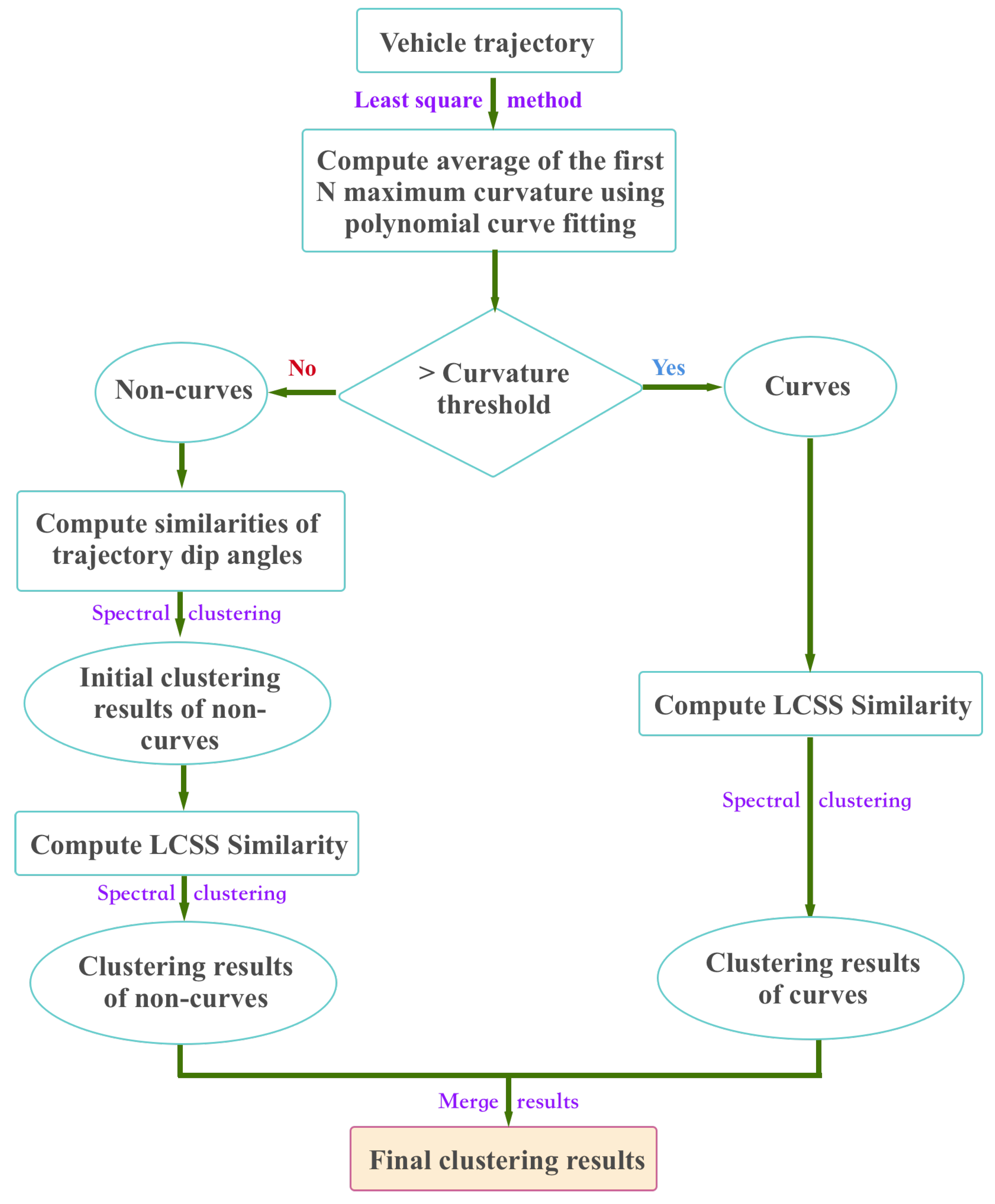
The proposed double spectral clustering (DSC) method proceeds as follows. Given a vehicle trajectory, we first compute its curvature via the least square and polynomial fitting method and take the average values of the first N curvatures as the final result. We then treat the trajectory as a curve (i.e., a vehicle taking turns) if its curvature is larger than the threshold , and treat it as a non-curve (i.e., vehicle going straight) otherwise. For curves, we directly construct the affinity matrix using the LCSS [40] and perform spectral clustering. For non-curves, we tackle them in two stages. In the first stage, we compute the similarity of their dip angles and perform spectral clustering to obtain the initial results. In the second stage, we construct the affinity matrix using the LCSS and perform spectral clustering again. Finally we merge the clustering results for curves and non-curves. The whole clustering workflow is illustrated in Figure 3.
The similarity between trajectory dig angles is defined as
where is the dig angle of the trajectory and is computed as
, k is the slope of the trajectory, and n is the number of trajectories.
3.2.2. Behavior Recognition by Classification
In this section, we approach the behavior recognition by supervised classification. Different from traditional approaches which incorporating Hidden Markov Modeling and other classification methods such as random forest and k nearest neighbor, we design a novel deep learning model based on Long Short-Term Memory (LSTM) [41]. As a special type of Recurrent Neural Networks (RNNs) [42], LSTM can effectively model the inherent structure of the sequential data and is proved to be powerful in many sequential classification problems [43,44,45].
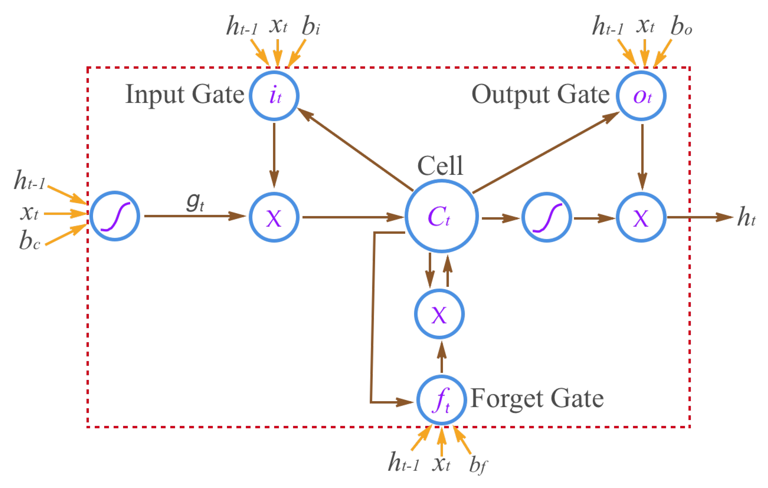
Network Structure. The basic structure of LSTM is depicted in Figure 4. The LSTM has a memory named “cell” to store the state vector which summarizes the sequence of the past input data. The current state is updated according to the current input, output, and the previous state stored in that “cell”. LSTM has a gate control mechanism that allows the network to “forget” the past state stored in cells or to learn the time stamp to update its state according to the new state information. Denoting as the state of the memory cell at the time step t, then is updated by
where is the sigmoid function, and means element-wise product. are the weight matrices for linear transformation. , , , are the bias vectors. is the input gate vector, is the forget gate vector, is the output gate vector, is state update vector, and is the output hidden state vector.
The input gate and the forget gate can control the information flow from the input to the output, respectively. Note that the behavior of the gate control is learned from data as well. Due to their recurrent nature, even a single layer of LSTM nodes can be considered a “deep” neural network.
The input gate and the forget gate can control the information flow from the input to the output, respectively. Note that the behavior of the gate control is learned from data as well. Due to their recurrent nature, even a single layer of LSTM nodes can be considered as a “deep” neural network.
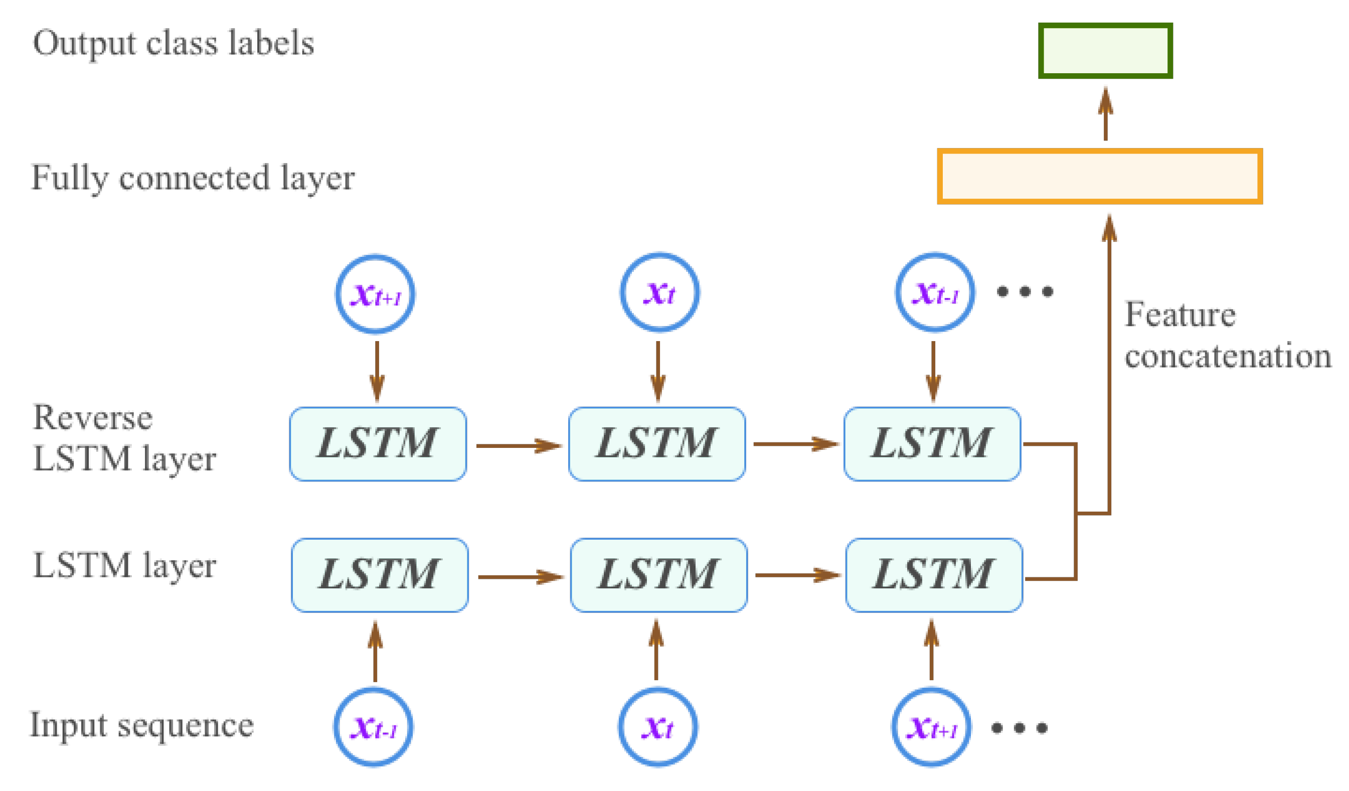
For many sequence classification tasks, it is beneficial to have access to future as well as past contexts. However, standard LSTM networks process sequences in temporal order and ignore past contexts. Bidirectional LSTM (BiLSTM) networks extend the standard LSTM networks by introducing a second layer where the hidden-to-hidden connections flow in opposite temporal order. The bidirectional model is therefore able to exploit information both from the past and the future. In our work, we built a trajectory-based bidirectional LSTM model (T-BiLSTM) to classify vehicle trajectories. We merged the output of the two directions by vector concatenation, which generates double the number of outputs to the next layer. In order to extract the information relevant to the class labels, we added an additional output network to the hidden state . We used a fully connected(FC) layer and one softmax layer that contains the linear transformation of followed by the softmax function. We show our network structure in Figure 5.
Feature representation. The BiLSTM accepts sequential vectors as inputs, so we need to transform the road plane position information stored in trajectories into the sequential features according to the temporal order. General features such as the location coordinates and vehicle speed often contain noisy information since they are sensitive to the motions of vehicles. In our work, we used angular changes to capture the trajectory variations due to its superior robustness compared to other types of features.
Let be the trajectory coordinates of a vehicle at time step t and be its coordinates at time step . The direction angle can then be calculated by
To build the trajectory features, first we resampled the trajectory to a unique length of N trajectory points. More specifically, we computed the overall length of trajectory M, then divided it into segments, each of which has length L. We then rechecked the distance between each adjacent point in M and linearly inserted a new point if their distance was larger than L. Each vehicle trajectory consisted of N points.
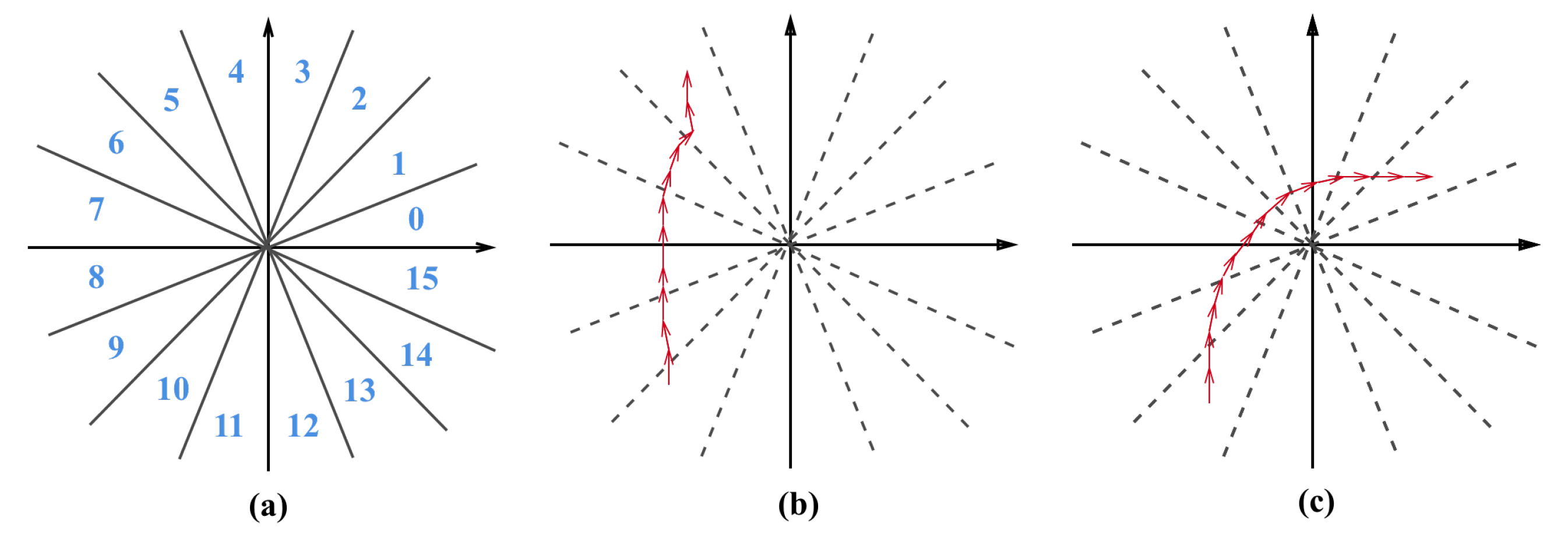
Second, we encoded and quantized the trajectory based on angular changes on 16 different directions with an interval of , as depicted in Figure 6a. For example, the sequential angle changes of a vehicle going straight could be encoded as “3-3-3-3-3-3-3-3-3-3-3-2-2-2-2-3-3-3-3-3” (b), and a vehicle turning right could be encoded as “3-3-7-7-3-3-7-3-7-7-7-7-7-15-7-15-7-7-15” (c).
At last, we normalized the features values to and used them as the input of the T-BiLSTM model.
Training. We formulated the behavior recognition problem as a multi-class classification problem where one class label was predicted given the sequential features of a testing vehicle’s trajectory. To train the T-BiLSTM, we minimized the negative log-likelihood function:
where w refers to the parameter of the neural network, J is the number of training samples, is the entry of , denotes the output of the softmax layer associated by class label , and is the regularization term controlled by the parameter .
4. Experiment and Discussion
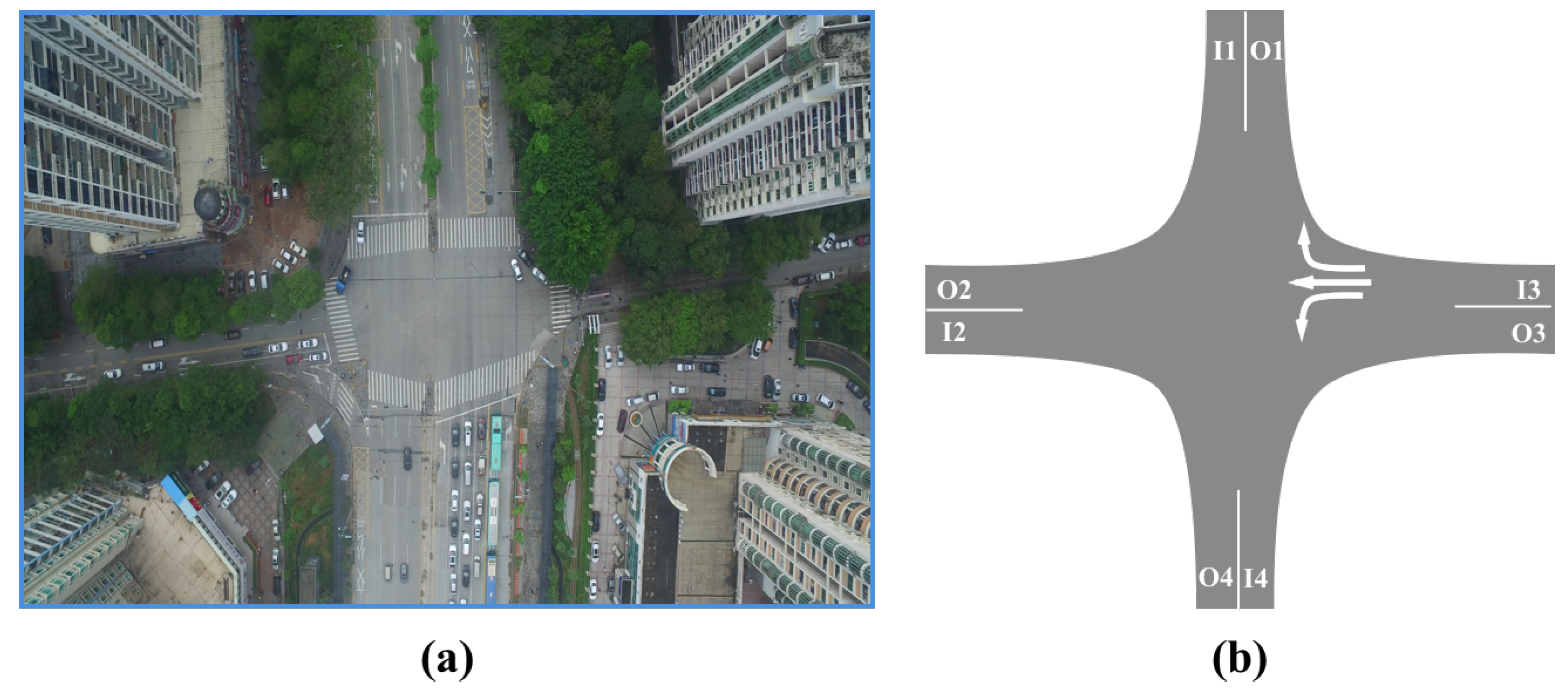
To evaluate the proposed framework, we captured a 14 m long traffic video with 4K resolution at a busy road intersections of a modern megacity by flying a UAV during the rush hours. The fps was 30 and the total number of frames was 25,200. The traffic scene at this intersection is shown in Figure 7.
To build the training set, we first temporally subsampled the original video frames by a factor of 150. For each frame in the subset, we then divided it into small patches with a uniform size of . We allowed an overlapping area of 200 pixel vertically and horizontally between these patches to ensure each vehicle appeared as a complete object. We then obtained 3400 training images. Next, we manually annotate vehicles with the following information: (a) bounding box: a rectangle surrounding each vehicle; (b) vehicle type: three general types including car, bus, and truck. This yielded 10,904 annotated vehicles. We used this dataset to train the RetinaNet object detector.
For testing, we collected another short video at the same road intersection but at a different time. The length of the testing video is 2 m and 47 s, with a resolution and 30 fps. The total number of frames was 5010.
4.1. Vehicle Trajectory Extraction
4.1.1. Vehicle Detection
We conducted the vehicle counting experiment to evaluate the effectiveness of the RetinaNet for vehicle detection. More concretely, we counted all types of vehicles in a randomly selected frame from the testing video.
Settings. In the training phase, we randomly selected 85% of these training images for training and the remaining 15% for validation. We compared RetineNet with another three recent deep-learning-based object detection methods: the you-only-look-once version 3 (YOLOv3) [46], the single shot multi-box detector (SSD) [47], and the faster regional convolutional neural network (Faster-RCNN) [48]. We trained the four deep models using Caffe [49] toolkit on a GTX 1080Ti GPU with 11 GB of video memory. The optimizer was set to stochastic gradient descent (SGD) for better performance. We initialized the learning rate at 0.001, and it began to decrease to one-tenth of the current value after 20,000 epochs. The total number of epochs was set to 120,000, and the momentum was set to 0.9 by default according to these models.
In the testing phase, the testing image was first divided into small patches () with an overlap of 200 pixels, and these patches were then fed into the trained network to detect vehicles. The global result was obtained by aggregating detection results on all patches. We eliminated the repeated bounding boxes on each vehicle by setting the center distance threshold as 0.3 and the IoU threshold as 0.1, respectively (determined by cross validation).
Evaluation. To make vehicle counting more straightforward, the detection result was visualized by drawing vehicle locations and corresponding types on the input image. Counting was done naturally by measuring the number of these bounding boxes. We quantitatively evaluated the counting result via precision, sensitivity, and quality, which are defined in [50]. True positives (TPs) are correctly detected vehicles, false positives (FPs) are invalid detections, and false negatives (FNs) are missed vehicles. Among the three evaluation criteria, quality is most important since it considers both the precision and the sensitivity of detection algorithms.
Result and discussion. We report the counting result on the testing image (see Table 1). It can be seen that the RetinaNet achieves the best performance, followed by YOLOv3 and SSD. The Faster-RCNN method yields too many false negatives (missing vehicles), which leads to low sensitivity and quality scores.
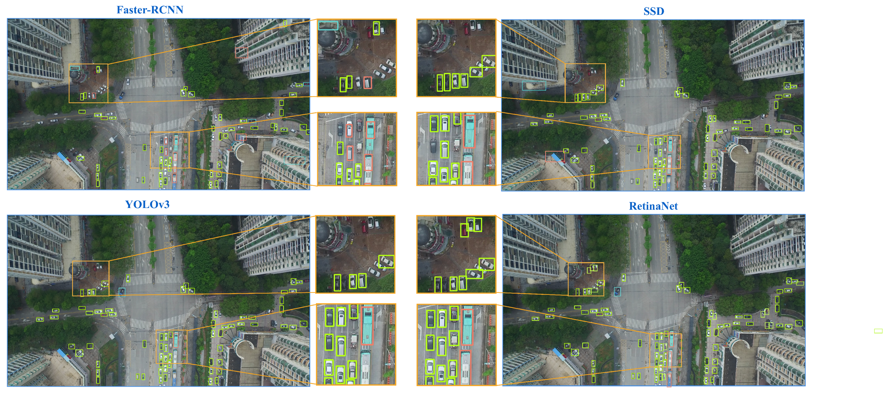
We visualize the results on the testing image (see Figure 8). Cars, buses, and trucks (if any) are automatically marked with light green, orange, and light blue bounding boxes, respectively. The small images in the middle are patches extracted from the original images, which give clearer ground details for type-specific detection. We noticed that SSD and Faster-RCNN generate a small number of false positives. This is to be expected, because in the training set, only regions containing vehicles are annotated by human annotators, while non-vehicle areas (including pure background and empty road) are ignored. A few ignored regions may exhibit very similar appearances with particular vehicles (especially buses and trucks), which would consequently lead to a few wrong detections.
We also provide the training time and the testing speed (frame per second) in Table 2. It can be observed that training of the Faster-RCNN model takes the longest time, but the testing speed is the lowest. The YOLOv3 model achieves the lowest training time and the fastest testing speed, which is due to its shallow network architecture compared with other models. However, its detection performance is worse than the RetinaNet model.
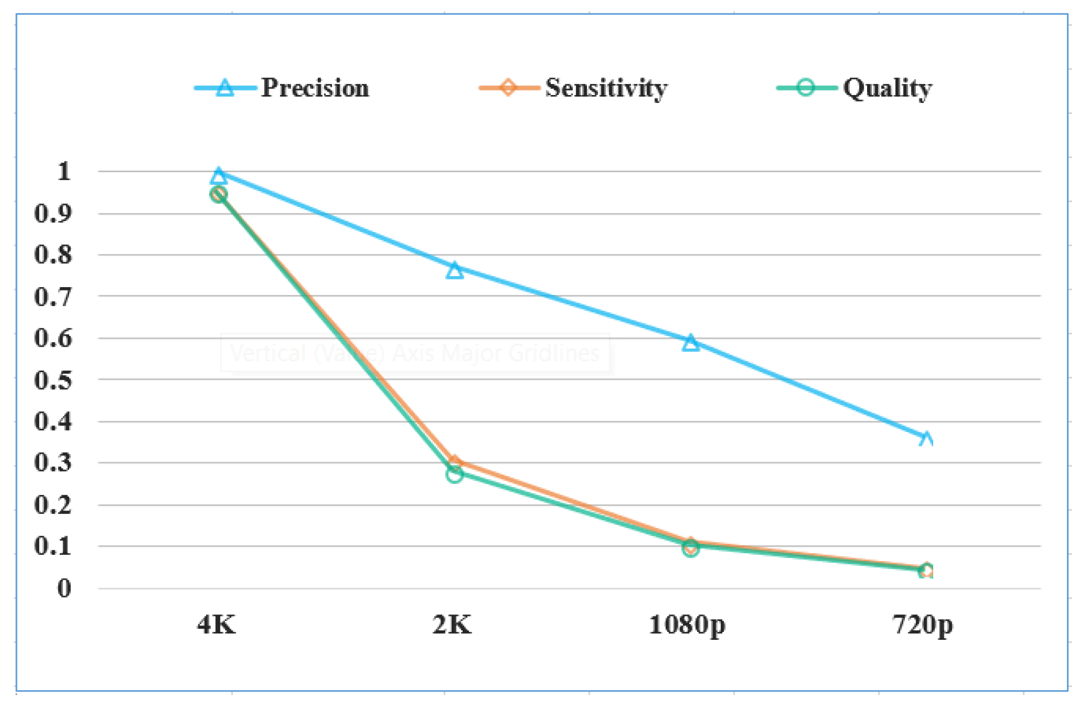
4.1.2. The Impact of Image Resolution
Although our data was recorded using 4K resolution, we are interested in determining if a high resolution really benefits the detection results. To do this, we created an auxiliary set where we down-sample the testing image. By adjusting the resolution of each image, we can determine performance changes of the detection algorithms. More specifically, we resized the original testing image to a resolution of 2K (2560), 1080p (), and 720p (), respectively. We then detected vehicles in these low-resolution images using the RetinaNet model.
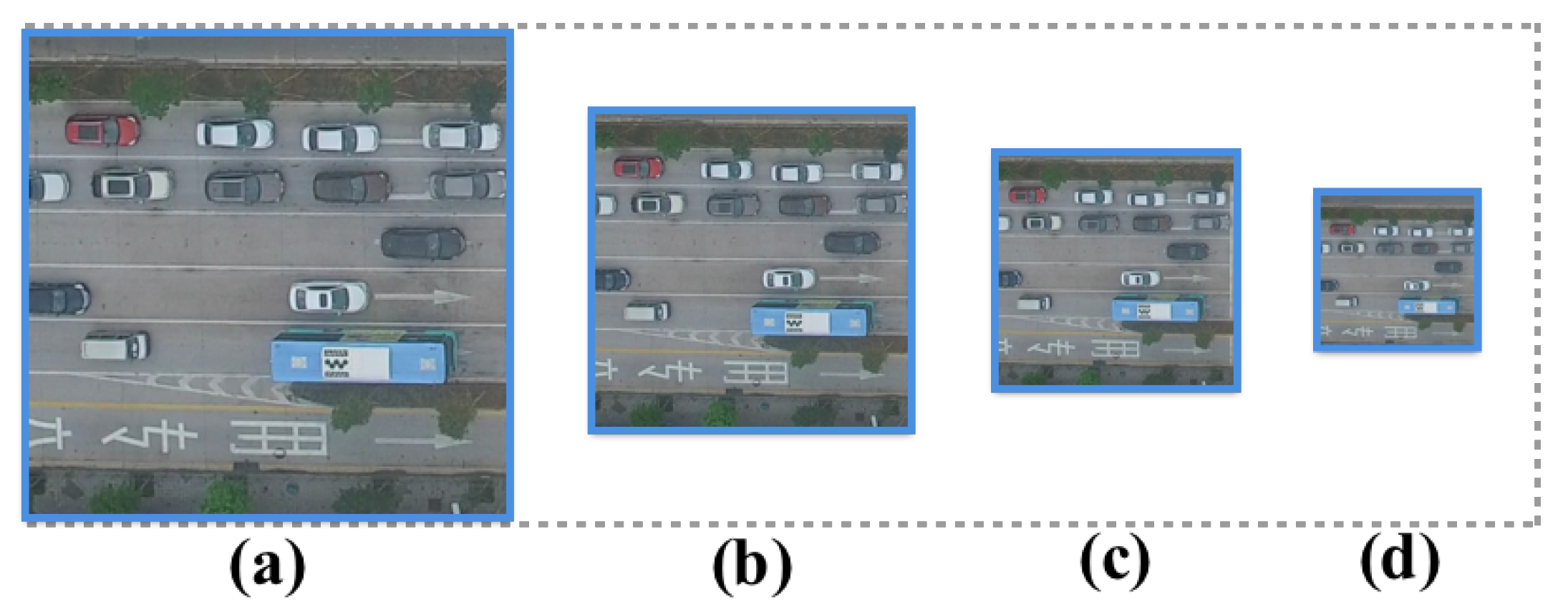
The results are shown in Figure 9. It can be seen that the detection performance degrades dramatically when the image resolution goes down, especially for the sensitivity measure and the quality measure. This makes sense because, in a 4K image, a vehicle generally takes a few pixels. However, in a 720p image, it only takes one or two pixels. This makes these vehicles (especially small cars) totally unrecognizable (see Figure 10) for vision-based algorithms. Hence, recording data in a high resolution is necessary since it provides enough ground details to help the detection algorithms accurately localize different types of vehicles.
4.1.3. Vehicle Trajectory Modeling
Settings. We modeled vehicle trajectories according to the tracking results. Given the testing video, we performed frame-by-frame vehicle detection using the trained network. Once detection was complete, a set of trackers were created to associate bounding boxes with different vehicles across the whole video sequence. We empirically set the threshold as 0.3 to start a new track, and set as 10 to terminate a track.
During the tracking phase, vehicles which were not within the range of roads (e.g., parking lots) were ignored in the counting phase since they contribute nothing to estimate the city traffic density. We manually defined the road ranges, since testing videos contained large-range and complex traffic scenes. For implementation, we ran the tracking algorithm on the testing videos using an Intel i7-6700K CPU with 32 GB on-board memory.
Evaluation. To evaluate the performance of the trajectory modeling approach, we tracked the target vehicle in consecutive frames, and extracted the tracked center point of its bounding box in each frame. For the , we computed the trajectory modeling error between the tracked center point and the ground-truth center point (labeled by human annotators) using
Based on Equation (13), we can compute the overall error by adding the modeling error in each frame:
where n is the number of frame being tracked. This error E is quantified using the number of pixels, and it could be easily extend to the real value of centimeters by multiplying it by a factor of 10 (i.e., the ground resolution is 10 cm/pixel).
We tracked all vehicles in the testing video and extracted 238 complete trajectories. The trajectories with unknown types were ignored. We then randomly selected 50 vehicles and computed their trajectory modeling errors using Equation (13). We took the average value as the modeling error of this frame. The modeling error of the whole testing video was then computed using Equation (14).
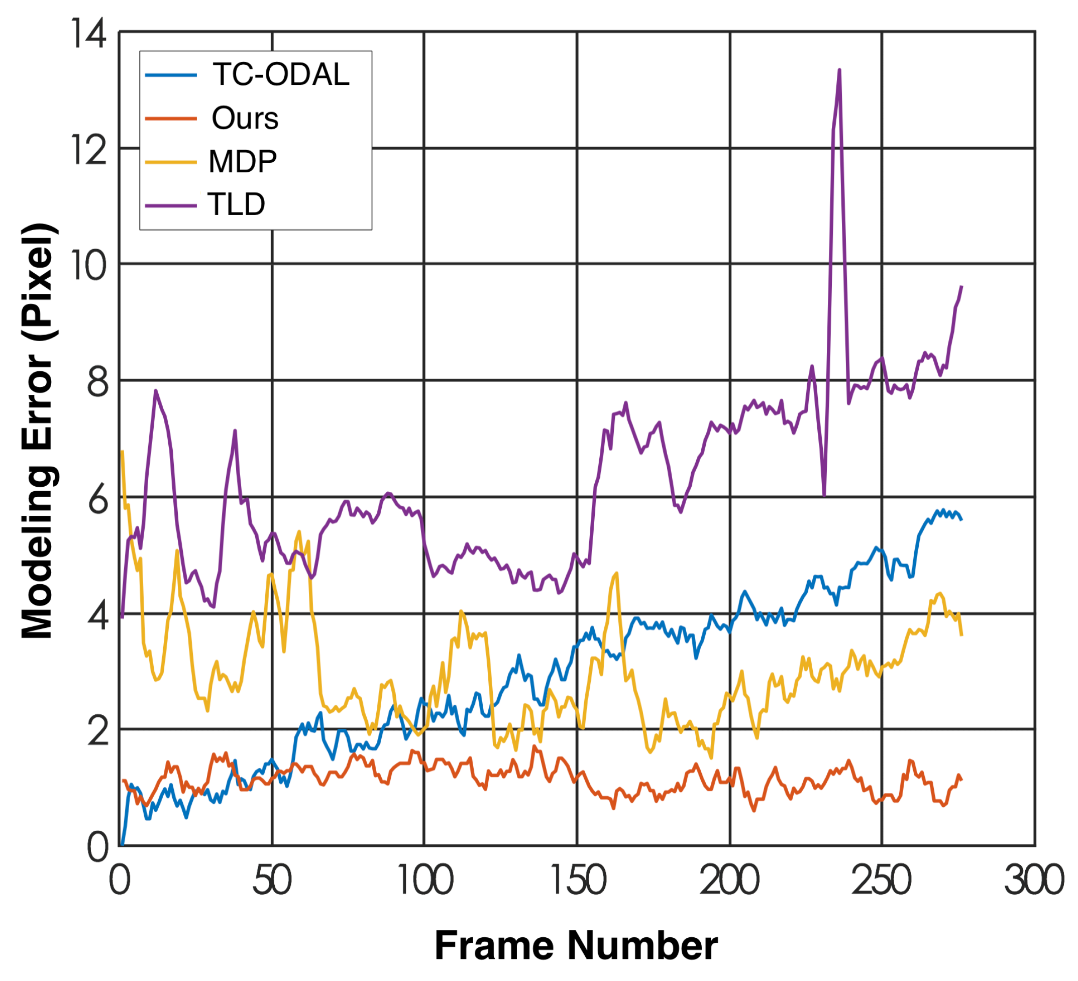
Since our modeling method is based on vehicle tracking, we used three other recent tracking approaches to model the vehicle trajectory and evaluate their performance for comparison, namely, tracking-learning-detection (TLD) [51], tracklet confidence and online discriminative appearance learning (TC-ODAL) [52], and the Markov decision process (MDP) [53]. In other words, our objective was to model the vehicle trajectories using the four methods and then evaluate their performance by computing the modeling error.
Result and discussion. We illustrate the frame-based trajectory modeling error for the first 280 frames of the testing video in Figure 11 and report the overall error in Table 3. It can be seen that our method outperformed the other three approaches in terms of both frame-based error and the overall error. The TLD method performed worst in this experiment, probably due to the lack of tracking information, since this method does not perform frame-by-frame vehicle detection on the video sequence. Fluctuations of the modeling error could be observed from the results of all four methods, but the error fluctuation range of our method was the smallest compared to the other three ones.
We also provide the tracking speed (frame per second) of the aforementioned approaches (see Table 4). Since we already have the frame-by-frame detection results, we can treat the tracking problem as the data association problem and do not need to train the algorithm. It can be seen that all the approaches achieve a relatively high tracking speed (i.e., above 55 fps), and the proposed method achieves the highest speed (i.e., 82.5 fps) as well as the lowest tracking error.
4.2. Vehicle Behavior Recognition
4.2.1. Behavior Recognition by Nearest Neighbor Search
Settings. For training, we built a training set by extracting 973 complete vehicle trajectories from the training video. Five hundred forty-two of them were with the type “go straight”, 204 of them were with the type “turn left”, and the remaining 227 were with the type “turn right”. For testing, we used 238 trajectories obtained from the testing video.
We applied the proposed double spectral clustering (DSC) on all the 973 trajectories and identified their types (i.e., go straight, right turn, and left turn). Given a testing trajectory, we determined its category based on a nearest neighbor search. We also performed two other clustering methods for comparison, one was a K-Means clustering based on LCSS similarity and the other one was normal spectral clustering based on LCSS similarity.
Evaluation. We employed the normalized accuracy metric considering the large variation in the number of samples in each trajectory type (most of them were of the type “going straight”). We first computed the accuracy within each class and then averaged them over all classes:
Result and discussion. The results are listed in Table 5. We noticed that our approach achieved an overall accuracy of 0.899, which is pretty high considering the complex road structure. In addition, the recognition accuracy of vehicle going straight is 0.910, followed by the the accuracy of “left turn” and “right turn”, achieving 0.857 and 0.882, respectively. On each class, our DSC method outperformed the other two methods, which demonstrates the effectiveness of our approach for unsupervised vehicle behavior recognition.
The training time and testing speed of these three approaches are shown in Table 6. It can be seen that the LCSS-KMeans runs faster than other methods, this is due to the relatively simpler complexity of the KMeans algorithm (the time complexity of KMeans is , while the time complexity of spectral clustering is ). However, the performance of LCSS-KMeans is worse than the proposed DSC method. In addition, the three methods achieve a very similar testing speed, because they have roughly the same sizes of searching space.
4.2.2. Behavior Recognition by Bidirectional Long Short-Term Memory
In this test, we performed behavior recognition using the proposed T-BiLSTM model.
Settings. We used the same training and testing data as in the previous section. For feature representation, we resampled the length of each trajectory to 256 points, and computed the sequences of angular changes for them. We followed [41] and employed the “back propagation through time” (BPTT) algorithm with a mini-batch size of 32 to train the network. For implementation, we used the Keras [54] deep learning toolkit for Python using Tensorflow [55] as backend.
For comparison, we trained five other models using our training data, namely a Hidden Markov Model (HMM) [56], an Activity Hidden Markov Model (A-HMM) [57], a Hidden Markov Model with Support Vector Machine (HMM-SVM) [58], a Hidden Markov Model with Random Forest (HMM-RF) [58], and normal LSTM [59]. The first four algorithms were trained on the CPU (i7-6700K), while the normal LSTM and our method were trained on the GPU (GTX 1080Ti). For evaluation, we used the normalized accuracy metric again.
Results and discussion. Table 7 presents the classification accuracy of each method on the testing data. Our approach outperformed all other methods in terms of both single class performance and overall performance. To be more specific, our T-BiLSTM achieved an accuracy of 0.965 on the “go straight” types, probably because the structure of the trajectories under this type are relatively easy to be temporally modeled and recognized. The accuracies decrease on the other two trajectory types due to the increased structural complexity. The LSTM method achieves the second highest accuracy, followed by HMM-RF and A-HMM.
We also show the training time and testing speed of these methods in Table 8. It can be seen that the training time of our method on the GPU is the lowest among the six trajectory classification approaches. For fair comparison, we also provide the training time of two deep-learning-based methods (LSTM [59] and ours) on the CPU side, which is much lower than on the GPU side. For testing speed, the HMM achieves the highest speed, but its classification performance is significantly worse than our method.
5. Concluding Remarks
A deep vehicle behavior recognition framework is proposed in this paper for urban vehicle behavior analysis in UAV videos. The improvements and contributions in this study mainly focus on four aspects: (1) we expand the vehicle behavior analysis area to the whole traffic network at road intersections, not individual road sections; (2) to recognize vehicle behaviors, we propose a nearest-neighbor-search-based model and a deep BiLSTM-based architecture considering both forward and backward dependencies of network-wide traffic data; (3) multiple influential factors for the proposed model are carefully analyzed; (4) we combine deep-learning-based methods and traditional algorithms to effectively balance the speed and accuracy of the proposed framework.
In recent years, the rapid development of autonomous car technologies and driving safety support systems have attracted considerable attention as solutions for preventing car crashes. The implementation of technologies in the intelligent transportation system to assist drivers in recognizing driving behaviors around their own vehicles can be expected to decrease accident rates. Car crashes often occur when traffic participants attempt to change lanes or make turns. Hence, vehicle behavior recognition exhibits significant importance in our daily lives. In our work, we mainly use vehicle trajectory analysis to help recognize three types of vehicle behaviors, but vehicle trajectory analysis also has more applications which we will consider in future work: for example, illegal lane changes, violations of traffic lines, overtaking in prohibited places, and illegal retrograde. We will also implement an artificial-intelligence-based transportation analytical platform and integrate it into the existing intelligent transportation system in order to improve the driving experience and safety of drivers.
Author Contributions
Conceptualization, K.S. and J.Z.; Methodology, K.S., S.J., J.Z. and G.Q.; Software, K.S. and W.L.; Validation, X.H. and G.Q.; Formal Analysis, X.H. and B.L.; Investigation, K.S. and W.L.; Resources, W.L., Writing—Original Draft Preparation, K.S. and J.Z.; Writing—Review & Editing, K.S., J.Z. and G.Q.
Conflicts of Interest
The authors declare no conflict of interest.
References
- Choi, E.H. Crash Factors in Intersection-Related Crashes: An on-Scene Perspective; Technical Report; The National Highway Traffic Safety Administration: Washington, DC, USA, 2010. [Google Scholar]
- Miller, T.; Kolosh, K.; Fearn, K.; Porretta, K. Injury Facts; 2015 Edition; Technical Report; National Safety Council: Itasca, IL, USA, 2015. [Google Scholar]
- Kim, Z.; Malik, J. Fast vehicle detection with probabilistic feature grouping and its application to vehicle tracking. In Proceedings of the Ninth IEEE International Conference on Computer Vision, Nice, France, 13–16 October 2003; p. 524. [Google Scholar]
- Morris, B.T.; Trivedi, M.M. A survey of vision-based trajectory learning and analysis for surveillance. IEEE Trans. Circuits Syst. Video Technol. 2008, 18, 1114–1127. [Google Scholar] [CrossRef]
- Cucchiara, R.; Piccardi, M.; Mello, P. Image analysis and rule-based reasoning for a traffic monitoring system. IEEE Trans. Intell. Transp. Syst. 2000, 1, 119–130. [Google Scholar] [CrossRef]
- Wang, L.; Chen, F.; Yin, H. Detecting and tracking vehicles in traffic by unmanned aerial vehicles. Autom. Constr. 2016, 72, 294–308. [Google Scholar] [CrossRef]
- Brooks, C.; Dobson, R.; Banach, D.; Dean, D.; Oommen, T.; Wolf, R.; Havens, T.; Ahlborn, T.; Hart, B. Evaluating the Use of Unmanned Aerial Vehicles for Transportation Purposes; Technical Report; Department of Transportation (MDOT): Michigan City, IN, USA, 2015. [Google Scholar]
- Zhou, H.; Kong, H.; Wei, L.; Creighton, D.C.; Nahavandi, S. Efficient Road Detection and Tracking for Unmanned Aerial Vehicle. IEEE Trans. Intell. Transp. Syst. 2015, 16, 297–309. [Google Scholar] [CrossRef]
- Hinz, S. Detection and counting of cars in aerial images. In Proceedings of the 2003 International Conference on Image Processing, Barcelona, Spain, 14–17 September 2003; Volume 3, pp. 997–1000. [Google Scholar]
- Yao, W.; Stilla, U. Comparison of two methods for vehicle extraction from airborne LiDAR data toward motion analysis. IEEE Geosci. Remote Sens. Lett. 2011, 8, 607–611. [Google Scholar] [CrossRef]
- Mundhenk, T.N.; Konjevod, G.; Sakla, W.A.; Boakye, K. A large contextual dataset for classification, detection and counting of cars with deep learning. In Proceedings of the European Conference on Computer Vision, Amsterdam, The Netherlands, 8–16 October 2016; pp. 785–800. [Google Scholar]
- Coifman, B.; McCord, M.; Mishalani, R.G.; Redmill, K. Surface transportation surveillance from unmanned aerial vehicles. In Proceedings of the 83rd Annual Meeting of the Transportation Research Board, Washington, DC, USA, 11–15 January 2004. [Google Scholar]
- Puri, A. A Survey of Unmanned Aerial Vehicles (UAV) for Traffic Surveillance; Department of Computer Science and Engineering, University of South Florida: Tampa, FL, USA, 2005; pp. 1–29. [Google Scholar]
- Moranduzzo, T.; Melgani, F. Automatic car counting method for unmanned aerial vehicle images. IEEE Trans. Geosci. Remote Sens. 2014, 52, 1635–1647. [Google Scholar] [CrossRef]
- Salvo, G.; Caruso, L.; Scordo, A. Urban traffic analysis through a UAV. Procedia-Soc. Behav. Sci. 2014, 111, 1083–1091. [Google Scholar] [CrossRef] [Green Version]
- Kanistras, K.; Martins, G.; Rutherford, M.J.; Valavanis, K.P. Survey of unmanned aerial vehicles (UAVs) for traffic monitoring. In Handbook of Unmanned Aerial Vehicles; Springer: Dordrecht, The Netherlands, 2015; pp. 2643–2666. [Google Scholar]
- Gallagher, K.; Lawrence, P. Unmanned systems and managing from above: the practical implications of UAVs for research applications addressing urban sustainability. In Urban Sustainability: Policy and Praxis; Springer: Cham, Switzerland, 2016; pp. 217–232. [Google Scholar]
- Khan, M.A.; Ectors, W.; Bellemans, T.; Janssens, D.; Wets, G. UAV-Based Traffic Analysis: A Universal Guiding Framework Based on Literature Survey. Transp. Res. Procedia 2017, 22, 541–550. [Google Scholar] [CrossRef]
- Coifman, B.; McCord, M.; Mishalani, R.G.; Iswalt, M.; Ji, Y. Roadway traffic monitoring from an unmanned aerial vehicle. IEE Proc.-Intell. Transp. Syst. 2006, 153, 11–20. [Google Scholar] [CrossRef]
- Skoglar, P.; Orguner, U.; Törnqvist, D.; Gustafsson, F. Road target search and tracking with gimballed vision sensor on an unmanned aerial vehicle. Remote Sens. 2012, 4, 2076–2111. [Google Scholar] [CrossRef]
- Moranduzzo, T.; Melgani, F. Detecting Cars in UAV Images With a Catalog-Based Approach. IEEE Trans. Geosci. Remote Sens. 2014, 52, 6356–6367. [Google Scholar] [CrossRef]
- Lin, T.Y.; Goyal, P.; Girshick, R.; He, K.; Dollár, P. Focal loss for dense object detection. arXiv 2017, arXiv:1708.02002. [Google Scholar]
- Bobick, A.F.; Davis, J.W. The recognition of human movement using temporal templates. IEEE Trans. Pattern Anal. Mach. Intell. 2001, 23, 257–267. [Google Scholar] [CrossRef] [Green Version]
- Veeraraghavan, H.; Papanikolopoulos, N.P. Learning to recognize video-based spatiotemporal events. IEEE Trans. Intell. Transp. Syst. 2009, 10, 628–638. [Google Scholar] [CrossRef]
- Porter, B.E.; England, K.J. Predicting red-light running behavior: A traffic safety study in three urban settings. J. Saf. Res. 2000, 31, 1–8. [Google Scholar] [CrossRef]
- Kasper, D.; Weidl, G.; Dang, T.; Breuel, G.; Tamke, A.; Wedel, A.; Rosenstiel, W. Object-oriented Bayesian networks for detection of lane change maneuvers. IEEE Intell. Transp. Syst. Mag. 2012, 4, 19–31. [Google Scholar] [CrossRef]
- Hu, W.; Xiao, X.; Xie, D.; Tan, T. Traffic accident prediction using vehicle tracking and trajectory analysis. In Proceedings of the 2003 IEEE International Conference on Intelligent Transportation Systems, Shanghai, China, 12–15 October 2003; Volume 1, pp. 220–225. [Google Scholar]
- Song, H.S.; Lu, S.N.; Ma, X.; Yang, Y.; Liu, X.Q.; Zhang, P. Vehicle behavior analysis using target motion trajectories. IEEE Trans. Veh. Technol. 2014, 63, 3580–3591. [Google Scholar] [CrossRef]
- Barth, A.; Franke, U. Estimating the driving state of oncoming vehicles from a moving platform using stereo vision. IEEE Trans. Intell. Transp. Syst. 2009, 10, 560–571. [Google Scholar] [CrossRef]
- Saligrama, V.; Konrad, J.; Jodoin, P.M. Video anomaly identification. IEEE Signal Process. Mag. 2010, 27, 18–33. [Google Scholar] [CrossRef]
- Huang, H.; Cai, Z.; Shi, S.; Ma, X.; Zhu, Y. Automatic detection of vehicle activities based on particle filter tracking. In Proceedings of the Second Symposium International Computer Science and Computational Technology (ISCSCT ’09), Huangshan, China, 26–28 December 2009; pp. 381–384. [Google Scholar]
- Pucher, M.; Schabus, D.; Schallauer, P.; Lypetskyy, Y.; Graf, F.; Rainer, H.; Stadtschnitzer, M.; Sternig, S.; Birchbauer, J.; Schneider, W.; et al. Multimodal highway monitoring for robust incident detection. In Proceedings of the 13th International IEEE Conference on Intelligent Transportation Systems, Funchal, Portugal, 19–22 September 2010; pp. 837–842. [Google Scholar]
- Lin, T.Y.; Dollár, P.; Girshick, R.; He, K.; Hariharan, B.; Belongie, S. Feature pyramid networks for object detection. In Proceedings of the Computer Vision and Pattern Recognition (CVPR), Honolulu, HI, USA, 21–26 July 2017; Volume 1, p. 4. [Google Scholar]
- He, K.; Zhang, X.; Ren, S.; Sun, J. Deep residual learning for image recognition. In Proceedings of the IEEE Conference on Computer Vision and Pattern Recognition, Las Vegas Valley, NV, USA, 26 June–1 July 2016; pp. 770–778. [Google Scholar]
- Neubeck, A.; Van Gool, L. Efficient non-maximum suppression. In Proceedings of the 18th International Conference on Pattern Recognition (ICPR ’06), Hong Kong, China, 20–24 August 2006; Volume 3, pp. 850–855. [Google Scholar]
- Erhan, D.; Szegedy, C.; Toshev, A.; Anguelov, D. Scalable object detection using deep neural networks. In Proceedings of the IEEE Conference on Computer Vision and Pattern Recognition, Columbus, OH, USA, 24–27 Jun 2014; pp. 2147–2154. [Google Scholar]
- Girshick, R. Fast r-cnn. In Proceedings of the IEEE International Conference on Computer Vision, Washington, DC, USA, 7–13 December 2015; pp. 1440–1448. [Google Scholar]
- Kalman, R.E. A new approach to linear filtering and prediction problems. J. Basic Eng. 1960, 82, 35–45. [Google Scholar] [CrossRef]
- Mills-Tettey, G.A.; Stentz, A.; Dias, M.B. The Dynamic Hungarian Algorithm for the Assignment Problem with Changing Costs; Carnegie Mellon University: Pittsburgh, PA, USA, 2007. [Google Scholar]
- Atev, S.; Miller, G.; Papanikolopoulos, N.P. Clustering of vehicle trajectories. IEEE Trans. Intell. Transp. Syst. 2010, 11, 647–657. [Google Scholar] [CrossRef]
- Hochreiter, S.; Schmidhuber, J. Long short-term memory. Neural Comput. 1997, 9, 1735–1780. [Google Scholar] [CrossRef] [PubMed]
- Kamijo, K.i.; Tanigawa, T. Stock price pattern recognition—A recurrent neural network approach. In Proceedings of the 1990 IJCNN International Joint Conference on Neural Networks, San Diego, CA, USA, 17–21 June 1990; pp. 215–221. [Google Scholar]
- Tai, K.S.; Socher, R.; Manning, C.D. Improved semantic representations from tree-structured long short-term memory networks. arXiv 2015, arXiv:1503.00075. [Google Scholar]
- Hanson, J.; Yang, Y.; Paliwal, K.; Zhou, Y. Improving protein disorder prediction by deep bidirectional long short-term memory recurrent neural networks. Bioinformatics 2016, 33, 685–692. [Google Scholar] [CrossRef] [PubMed]
- Zhou, P.; Shi, W.; Tian, J.; Qi, Z.; Li, B.; Hao, H.; Xu, B. Attention-based bidirectional long short-term memory networks for relation classification. In Proceedings of the 54th Annual Meeting of the Association for Computational Linguistics, Berlin, Germany, 7–12 August 2016; Volume 2, pp. 207–212. [Google Scholar]
- Redmon, J.; Farhadi, A. YOLOv3: An Incremental Improvement. arXiv 2018, arXiv:1804.02767. [Google Scholar]
- Liu, W.; Anguelov, D.; Erhan, D.; Szegedy, C.; Reed, S.; Fu, C.Y.; Berg, A.C. Ssd: Single shot multibox detector. In Proceedings of the European Conference on Computer Vision, Amsterdam, The Netherlands, 8–16 October 2006; Springer: Cham, Switzerland, 2016; pp. 21–37. [Google Scholar]
- Ren, S.; He, K.; Girshick, R.; Sun, J. Faster R-CNN: Towards real-time object detection with region proposal networks. In Proceedings of the Advances in Neural Information Processing Systems, Montreal, QC, Canada, 7–12 December 2015; pp. 91–99. [Google Scholar]
- Jia, Y.; Shelhamer, E.; Donahue, J.; Karayev, S.; Long, J.; Girshick, R.; Guadarrama, S.; Darrell, T. Caffe: Convolutional architecture for fast feature embedding. In Proceedings of the 22nd ACM International Conference on Multimedia, Orlando, FL, USA, 3–7 November 2014; pp. 675–678. [Google Scholar]
- Leitloff, J.; Rosenbaum, D.; Kurz, F.; Meynberg, O.; Reinartz, P. An operational system for estimating road traffic information from aerial images. Remote Sens. 2014, 6, 11315–11341. [Google Scholar] [CrossRef] [Green Version]
- Kalal, Z.; Mikolajczyk, K.; Matas, J. Tracking-Learning-Detection. IEEE Trans. Pattern Anal. Mach. Intell. 2012, 34, 1409–1422. [Google Scholar] [CrossRef] [PubMed] [Green Version]
- Bae, S.H.; Yoon, K.J. Robust online multi-object tracking based on tracklet confidence and online discriminative appearance learning. In Proceedings of the IEEE Conference on Computer Vision and Pattern Recognition, Columbus, OH, USA, 23–28 June 2014; pp. 1218–1225. [Google Scholar]
- Xiang, Y.; Alahi, A.; Savarese, S. Learning to track: Online multi-object tracking by decision making. In Proceedings of the 2015 IEEE International Conference on Computer Vision (ICCV), Santiago, Chile, 7–13 December 2015; pp. 4705–4713. [Google Scholar]
- Chollet, F. Github. Available online: https://github.com/fchollet/keras (accessed on 5 June 2018).
- Abadi, M.; Barham, P.; Chen, J.; Chen, Z.; Davis, A.; Dean, J.; Devin, M.; Ghemawat, S.; Irving, G.; Isard, M.; et al. TensorFlow: A System for Large-Scale Machine Learning. In Proceedings of the 12th USENIX Symposium on Operating Systems Designand Implementation (OSDI ’16), Savannah, GA, USA, 2–4 November 2016; Volume 16, pp. 265–283. [Google Scholar]
- Hervieu, A.; Bouthemy, P.; Le Cadre, J.P. A HMM-based method for recognizing dynamic video contents from trajectories. In Proceedings of the 2007 IEEE International Conference on Image Processing, San Antonio, TX, USA, 16 September–19 October 2007; Volume 4, pp. IV-533–IV-536. [Google Scholar]
- Morris, B.T.; Trivedi, M.M. Trajectory learning for activity understanding: Unsupervised, multilevel, and long-term adaptive approach. IEEE Trans. Pattern Anal. Mach. Intell. 2011, 33, 2287–2301. [Google Scholar] [CrossRef] [PubMed]
- Fan, Q.; Ruan, T.; Wu, J.; Dong, T. Vehicle Behavior Recognition Method Based on Quadratic Spectral Clustering and HMM-RF Hybrid Model. Comput. Sci. 2016, 43, 288–293. [Google Scholar]
- Altché, F.; De La Fortelle, A. An LSTM network for highway trajectory prediction. In Proceedings of the 2017 IEEE 20th International Conference on Intelligent Transportation Systems (ITSC), Yokohama, Japan, 16–19 October 2017; pp. 353–359. [Google Scholar]
Figure 1.
An illustration of the hierarchical structure of our work and its relationship to the intelligent transportation system (ITS). In the first stage, we used a UAV to collect high-resolution city traffic videos and, in Stage 2, extracted the static and dynamic information of road vehicles. In the third stage, we modeled and analyzed vehicle trajectory data, and observed vehicle behaviors. In our future work, all these achievements could contribute to the construction of comprehensive ITS services, such as traffic flow analysis, abnormal event detection, and security monitoring.

Figure 2.
The RetinaNet network architecture uses a Feature Pyramid Network (FPN) [33] backbone on top of a feedforward ResNet architecture [34] (a) to generate a rich, multi-scale convolutional feature pyramid (b). To this backbone, RetinaNet attaches two subnetworks, one for classifying anchor boxes (c) and one for regressing from anchor boxes to ground-truth object boxes (d).

Figure 3.
The working flow of the proposed double spectral clustering (DSC) method. For curve trajectories, we directly measure their pairwise similarities using the longest common sub-sequence similarity (LCSS) measure. For non-curve trajectories, we first cluster them according to the similarities of their dip angles, then use LCSS again to obtain the final results. Finally, we combine the clustering results on the two types of trajectories.

Figure 4.
The basic Long Short-Term Memory (LSTM) structure.

Figure 5.
The network structure of trajectory classification using bidirectional LSTM (BiLSTM).

Figure 6.
(a) The encoding and quantization of direction angles. (b) The changing angles of a vehicle going straight. (c) The changing angles of a vehicle turning right.
Figure 6.
(a) The encoding and quantization of direction angles. (b) The changing angles of a vehicle going straight. (c) The changing angles of a vehicle turning right.

Figure 7.
The traffic scene of the testing video. (a) The snapshot of the original video. (b) The sketch map of the intersection. The character “I” means “into the camera view” and the “O” means “out of the camera view.”
Figure 7.
The traffic scene of the testing video. (a) The snapshot of the original video. (b) The sketch map of the intersection. The character “I” means “into the camera view” and the “O” means “out of the camera view.”

Figure 8.
The qualitative result of vehicle detection on a testing image.

Figure 9.
Detection performance in different resolutions.

Figure 10.
Example of an image patch in different resolution: (a) 4K; (b) 2K; (c) 1080p; and (d) 720p.
Figure 10.
Example of an image patch in different resolution: (a) 4K; (b) 2K; (c) 1080p; and (d) 720p.

Figure 11.
The frame-based trajectory modeling errors (lower is better) for four methods. The horizontal axe denotes the frame number, and the vertical axe represents the error value measured in pixels.
Figure 11.
The frame-based trajectory modeling errors (lower is better) for four methods. The horizontal axe denotes the frame number, and the vertical axe represents the error value measured in pixels.


Table 1.
Quantitative results of vehicle counting in 4K testing image. For each testing image, we show the TP, FP, FN, precision, sensitivity, and quality. The best values are highlighted by bold typefaces. The up arrow means that higher is better, and the down arrow means that lower is better. The best values are highlighted using a bold typeface.
| Method | TP ↑ | FP ↓ | FN ↓ | Precision ↑ | Sensitivity ↑ | Quality ↑ |
|---|---|---|---|---|---|---|
| Faster-RCNN | 49 | 6 | 36 | 0.890 | 0.576 | 0.538 |
| SSD | 68 | 2 | 17 | 0.971 | 0.80 | 0.782 |
| YOLOv3 | 71 | 0 | 14 | 1.0 | 0.835 | 0.835 |
| RetinaNet | 81 | 0 | 4 | 1.0 | 0.953 | 0.953 |
Table 2.
Training time and testing speed of vehicle detection methods. The up arrow means that higher is better, while the down arrow means that lower is better. The best values are highlighted using a bold typeface.
Table 2.
Training time and testing speed of vehicle detection methods. The up arrow means that higher is better, while the down arrow means that lower is better. The best values are highlighted using a bold typeface.
| Model | Faster-RCNN | SSD | YOLOv3 | RetinaNet |
|---|---|---|---|---|
| Training Time ↓ | 37 h 29 m | 24 h 58 m | 18 h 29 m | 20 h 15 m |
| Testing Speed ↑ | 15.3 | 44.1 fps | 72.3 fps | 60.2 fps |
Table 3.
The overall trajectory modeling errors (lower is better) for four methods: tracking-learning-detection (TLD), tracklet confidence and online discriminative appearance learning (TC-ODAL), the Markov decision process (MDP), and ours. The error value is measured in pixels. The best value is highlighted using a bold typeface.
| TLD | TC-ODAL | MDP | Ours | |
|---|---|---|---|---|
| Overall Error (pixel) ↓ | 1743 | 796 | 632 | 316 |
Table 4.
The tracking speed (higher is better) of different methods. The best value is highlighted using a bold typeface.
Table 4.
The tracking speed (higher is better) of different methods. The best value is highlighted using a bold typeface.
| Method | TC-ODAL | MDP | TLD | Ours |
|---|---|---|---|---|
| Tracking speed (fps) | 78.9 | 65.1 | 58.4 | 82.5 |
Table 5.
The results of vehicle trajectory clustering for behavior recognition. For each type of behavior, we show the accuracy on each type and the average value (higher is better). The best values are highlighted using a bold typeface.
Table 5.
The results of vehicle trajectory clustering for behavior recognition. For each type of behavior, we show the accuracy on each type and the average value (higher is better). The best values are highlighted using a bold typeface.
| Bebavior | LCSS-KMeans | LCSS-Spectral | DSC (Ours) |
|---|---|---|---|
| Go straight | 0.813 | 0.802 | 0.910 |
| Right turn | 0.727 | 0.764 | 0.857 |
| Left turn | 0.667 | 0.769 | 0.882 |
| Average | 0.756 | 0.782 | 0.899 |
Table 6.
The training time (in seconds, lower is better) and testing speed (trajectory per second, higher is better) of the three methods. The best values are highlighted using a bold typeface.
Table 6.
The training time (in seconds, lower is better) and testing speed (trajectory per second, higher is better) of the three methods. The best values are highlighted using a bold typeface.
| Method | LCSS-KMeans | LCSS-Spectral | DSC (Ours) |
|---|---|---|---|
| Training Time (s) ↓ | 11.3 | 25.8 | 43.2 |
| Testing Speed (tps) ↑ | 62.1 | 57.5 | 55.6 |
Table 7.
The results of vehicle trajectory classification for behavior recognition. We show the accuracy on each type and the average value (higher is better). The best values are highlighted using a bold typeface.
Table 7.
The results of vehicle trajectory classification for behavior recognition. We show the accuracy on each type and the average value (higher is better). The best values are highlighted using a bold typeface.
| Behavior | HMM | A-HMM | HMM-RF | HMM-SVM | LSTM | T-BiLSTM (Ours) |
|---|---|---|---|---|---|---|
| Go straight | 0.825 | 0.893 | 0.931 | 0.832 | 0.924 | 0.965 |
| Right turn | 0.703 | 0.803 | 0.856 | 0.752 | 0.896 | 0.938 |
| Left turn | 0.671 | 0.733 | 0.832 | 0.714 | 0.875 | 0.916 |
| Average | 0.733 | 0.810 | 0.873 | 0.766 | 0.898 | 0.940 |
Table 8.
The training time (in seconds, lower is better) and the testing speed (trajectory per second) of these methods. The best values are highlighted using a bold typeface.
Table 8.
The training time (in seconds, lower is better) and the testing speed (trajectory per second) of these methods. The best values are highlighted using a bold typeface.
| Method | HMM | A-HMM | HMM-RF | HMM-SVM | LSTM (CPU/GPU) | T-BiLSTM (Ours) (CPU/GPU) |
|---|---|---|---|---|---|---|
| Training Time (s) ↓ | 296.4 | 331.1 | 395.7 | 388.5 | 1351.5/136.6 | 526.6/47.7 |
| Testing Speed (tps) ↑ | 65.2 | 62.1 | 59.9 | 58.1 | 37.1/40.3 | 38.2/59.2 |
© 2018 by the authors. Licensee MDPI, Basel, Switzerland. This article is an open access article distributed under the terms and conditions of the Creative Commons Attribution (CC BY) license (http://creativecommons.org/licenses/by/4.0/).
Share and Cite
MDPI and ACS Style
Zhu, J.; Sun, K.; Jia, S.; Lin, W.; Hou, X.; Liu, B.; Qiu, G. Bidirectional Long Short-Term Memory Network for Vehicle Behavior Recognition. Remote Sens. 2018, 10, 887. https://doi.org/10.3390/rs10060887
AMA Style
Zhu J, Sun K, Jia S, Lin W, Hou X, Liu B, Qiu G. Bidirectional Long Short-Term Memory Network for Vehicle Behavior Recognition. Remote Sensing. 2018; 10(6):887. https://doi.org/10.3390/rs10060887
Chicago/Turabian StyleZhu, Jiasong, Ke Sun, Sen Jia, Weidong Lin, Xianxu Hou, Bozhi Liu, and Guoping Qiu. 2018. "Bidirectional Long Short-Term Memory Network for Vehicle Behavior Recognition" Remote Sensing 10, no. 6: 887. https://doi.org/10.3390/rs10060887
Note that from the first issue of 2016, this journal uses article numbers instead of page numbers. See further details here.