A Deep Convolutional Generative Adversarial Networks (DCGANs)-Based Semi-Supervised Method for Object Recognition in Synthetic Aperture Radar (SAR) Images

Abstract

Synthetic aperture radar automatic target recognition (SAR-ATR) has made great progress in recent years. Most of the established recognition methods are supervised, which have strong dependence on image labels. However, obtaining the labels of radar images is expensive and time-consuming. In this paper, we present a semi-supervised learning method that is based on the standard deep convolutional generative adversarial networks (DCGANs). We double the discriminator that is used in DCGANs and utilize the two discriminators for joint training. In this process, we introduce a noisy data learning theory to reduce the negative impact of the incorrectly labeled samples on the performance of the networks. We replace the last layer of the classic discriminators with the standard softmax function to output a vector of class probabilities so that we can recognize multiple objects. We subsequently modify the loss function in order to adapt to the revised network structure. In our model, the two discriminators share the same generator, and we take the average value of them when computing the loss function of the generator, which can improve the training stability of DCGANs to some extent. We also utilize images of higher quality from the generated images for training in order to improve the performance of the networks. Our method has achieved state-of-the-art results on the Moving and Stationary Target Acquisition and Recognition (MSTAR) dataset, and we have proved that using the generated images to train the networks can improve the recognition accuracy with a small number of labeled samples.

1. Introduction

Synthetic Aperture Radar (SAR) can acquire the images of non-cooperative moving objects, such as aircrafts, ships, and celestial objects over a long distance under all weather and all day, which is now widely used in civil and military fields [1]. SAR images contain rich target information, but because of different imaging mechanisms, SAR images are not as intuitive as optical images, and it is difficult for human eyes to recognize objects in SAR images accurately. Therefore, SAR automatic target recognition technology (SAR-ATR) has become an urgent need, which is also a hot topic in recent years.

SAR-ATR mainly contains two aspects: target feature extraction and target recognition. At present, target features that are reported in most studies include target size, peak intensity, center distance, and Hu moment. The methods of target recognition include template matching, model-based methods, and machine learning methods [2,3,4,5,6,7,8,9,10,11,12,13,14,15]. Machine learning methods have attracted increasing attention because appropriate models can be formed while using these methods. Machine learning methods commonly used for image recognition include support vector machines (SVM), AdaBoost, and Bayesian neural network [16,17,18,19,20,21,22,23,24,25]. In order to obtain better recognition results, traditional machine learning methods require preprocessing images, such as denoising and feature extraction. Fu et al. [26] extracted Hu moments as the feature vectors of SAR images and used them to train SVM, and finally, achieved better recognition accuracy than directly training SVM with SAR images. Huan et al. [21] used a non-negative matrix factorization (NFM) algorithm to extract feature vectors of SAR images, and combined SVM and Bayesian neural networks to classify feature vectors. However, in these cases, how to select and combine features is a difficult problem, and the preprocessing scheme is rather complex. Therefore, these methods are not practice-friendly, although they are somehow effective.

In recent years, deep learning has achieved great successes in the field of object recognition in images. Its advantage lies in the ability of using a large amount of data to train the networks and to learn the target features, which avoid complex preprocessing and can also achieve better results. Numerous studies have brought deep learning into the field of SAR-ATR [27,28,29,30,31,32,33,34,35,36,37,38,39]. The most popular and effective model of deep learning is convolutional neural networks (CNNs), which is based on supervised learning, which requires a large number of labeled samples for training. However, in practical applications, people can only obtain unlabeled samples at first, and then label them manually. Semi-supervised learning enables the label prediction of a large number of unlabeled samples by training with a small number of labeled samples. Traditional semi-supervised methods in the field of machine learning include generative methods [40,41], semi-supervised SVM [42], graph semi-supervised learning [43,44], and difference-based methods [45]. With the introduction of deep learning, people begin to combine the classical statistical methods with deep neural networks to obtain better recognition results and to avoid complicated preprocessing. In this paper, we will combine traditional semi-supervised methods with deep neural networks, and propose a semi-supervised learning method for SAR automatic target recognition.

We intend to achieve two goals: one is to predict the labels of a large amount of unlabeled samples through training with a small amount of labeled samples and then extend the labeled set; and, the other one is to accurately classify multiple object types. To achieve the former target, we develop training methods of co-training [46]. In each training round, we utilize the labeled samples to train two classifiers, then use each classifier to predict the labels of the unlabeled samples respectively, and select those positive samples with high confidence from the newly labeled ones and add them to the labeled set for the next round of training. We propose a stringent rule when selecting positive samples to increase the confidence of the predicted labels. In order to reduce the negative influence of those wrongly labeled samples, we introduce the standard noisy data learning theory [47]. With advanced training processes, the recognition outcome of the classifier is getting better, and the number of the positive samples selected in each round of training is also increasing. Since the training process is supervised, we choose a CNN for the classifier due to the high performance on many other recognition tasks.

The core of our proposed method is to extend the labeled sample set with newly labeled samples, and to ensure that the extended labeled sample set enables the classifier to have better performance than the previous version. We have noticed the deep convolutional generative adversarial networks (DCGANs) [48], which is very popular in recent years in the field of deep learning. The generator can generate fake images that are very similar to the real images by learning the features of the real images. We expect to expand the sample set with high-quality fake images for data enhancement to better achieve our goals. DCGANs contains a generator and a discriminator. We double the discriminator and use the two discriminators for joint training to complete the task of semi-supervised learning. Since the discriminator of DCGANs cannot be used to recognize multiple object types, some adjustments to the network structure are required. Salimans et al. [49] proposed to replace the last layer of the discriminators with the softmax function to output a vector of the class probabilities. We draw on this idea and modify the classic loss function to achieve the adjustments. We also take the average value of the two classifier when computing the loss function of the generator, which have been proved to improve the training stability to some extent. We prove that our method performs better, especially when the number of the unlabeled samples is much greater than that of the labeled samples (which is a common scenario). By selecting high quality’s synthetically generated images for training, the recognition results are improved.

2. DCGANs-Based Semi-Supervised Learning

2.1. Framework

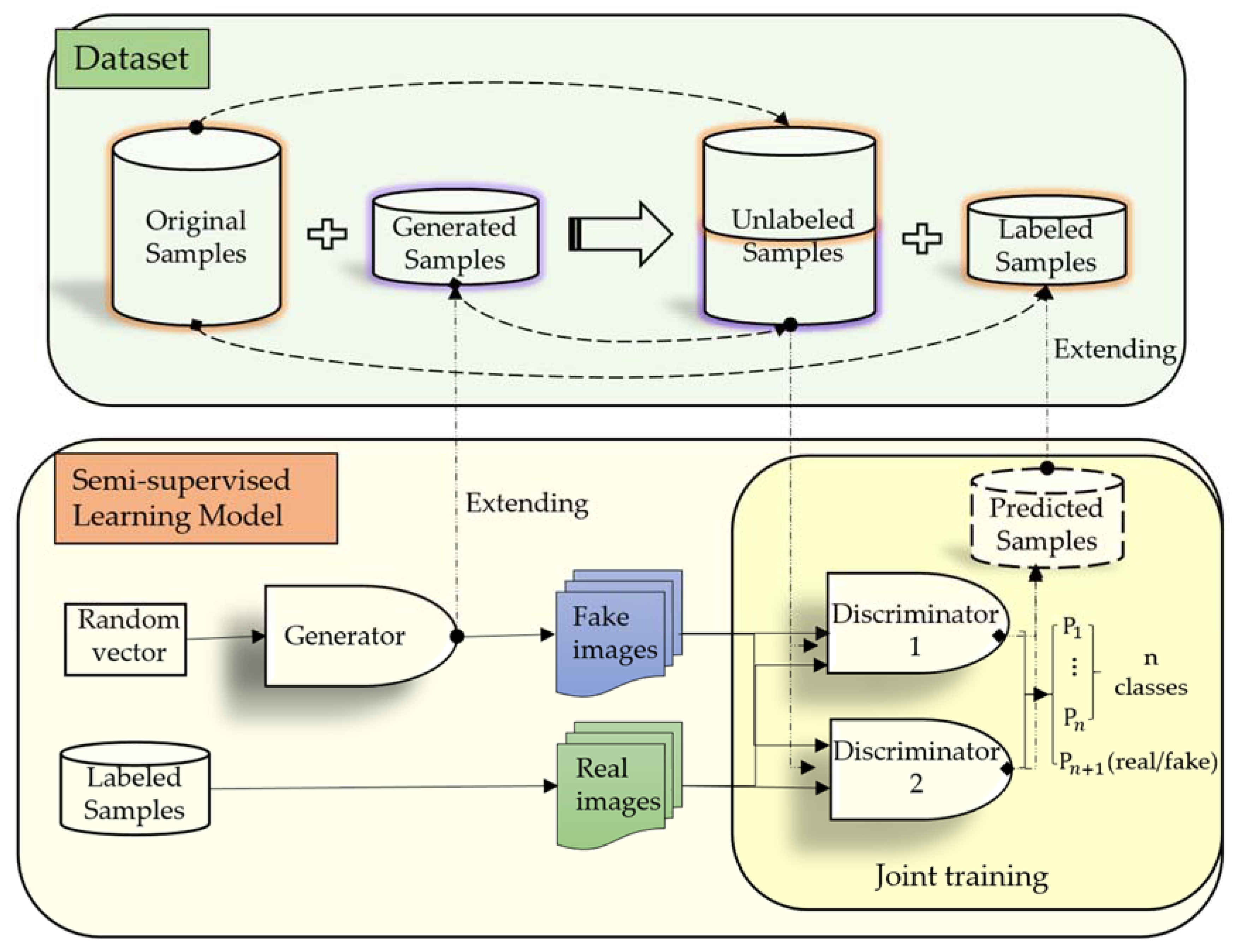
The framework of our method is shown in Figure 1. There are two complete DCGANs in the framework, each contains one generator and two discriminators. To recognize multiple object types, we replace the last layer of the discriminators with a softmax function, and output a vector of that class probabilities. The last value in the vector represents the probability that the input sample is fake, while the others represent the probabilities that the input sample is real and that it belongs to a certain class. We modify the loss function of the discriminators to adapt to the adjustments, and take the average value of them when computing the loss function of the generator. The process of semi-supervised learning is accomplished through joint training of the two discriminators, and the specific steps in each training round are as follows: we firstly utilize the labeled samples to train the two discriminators, then use each discriminator to predict the labels of the unlabeled samples, respectively. We select those positive samples with high confidence from the newly labeled ones, and finally add them to each other’s labeled set for the next round of training when certain conditions are satisfied.

The datasets used for training are constructed according to the experiments, and there are two different cases: the first is to directly divide the original dataset into a labeled sample set and an unlabeled sample set to verify the effectiveness of the proposed semi-supervised method; the second is to select specific generated images of high quality as the unlabeled sample sets, select a portion from the original dataset, and form the labeled sample set to verify the effect of using the generated false images to train the networks.

2.2. MO-DCGANs

The generator is a deconvolution neural network, whose input is a random vector and outputs a fake image that is very close to a real image by learning the features of the real images. While the discriminator of DCGANs is an improved convolutional neural network, and both fake and real images will be sent to the discriminator. The output of the discriminator is a number falling in the range of 0 and 1, if the input data is a real image then this output number is getting closer to 1, and if the input data is a fake image then this output number is getting closer to 0. Both the generator and the discriminator will be strengthened during the training process.

In order to recognize multiple object types, we conduct enhancement for the discriminators. Inspired by Salimans et al. [49], we replace the output of the discriminator with a softmax function and make it a standard classifier for recognizing multiple object types. We name this model multi-output-DCGANs (MO-DCGANs). Assuming that the random vector$z$has a uniform noise distribution$P_z\left(z\right)$, and$G\left(z\right)$maps it to the data space of the real images; the input$x$of the discriminator, which is assumed to have a distribution $P_{data}\left(x,y\right)$, is a real or fake image with label$y$. The discriminator outputs a$k+1$dimensional vector of logits$l=\left\{l_1,l_2,\cdots ,l_{k+1}\right\}$, which is finally turned into a$k+1$dimensional vector of class probabilities$p=\left\{p_1,p_2,\cdots ,p_{k+1}\right\}$by the softmax function:

$$p_j=\frac{e^{l_j}}{{\displaystyle {\sum }_{i=1}^{k+1}{e}^{l_i}}},j\in \left\{1,2,\cdots ,k+1\right\}$$

(1)

A real image will be discriminated as one of the former$k$classes, and a fake image will be discriminated as the$k+1$class.

We formulate the loss function of MO-DCGANs as a standard minimax game:

$$L=-{{\rm E}}_{x,y\sim P_{data}(x,y)}\left\{D(y|x,y<k+1)\right\}-{{\rm E}}_{x\sim G(z)}\left\{D(y|G(z),y=k+1)\right\}$$

(2)

We do not take the logarithm of$D\left(y|x\right)$directly in Equation (2), because the output neurons of the discriminator in our model have increased from 1 to$k+1$, and$D\left(y|x\right)$no longer represents the probability that the input is a real image but a loss function, corresponding to a more complicated condition. We choose cross-entropy function as the loss function, and then $D\left(y|x\right)$is computed as:

$$D\left(y|x\right)=-{\displaystyle \sum _i{y}_i^{\prime }}\log \left(p_i\right)$$

(3)

where$y^{\prime }$refers to the expected class, $p_i$represents the probability that the input sample belongs to $y^{\prime }$. It should be noted that$y$and$y^{\prime }$are one hot vectors. According to Equation (3), $D\left(y|x,y<k+1\right)$can be further expressed as Equation (4) when the input is a real image:

$$D\left(y|x,y<k+1\right)=-{\displaystyle \sum _{i=1}^k{y}^{\prime }\log \left(p_i\right)}$$

(4)

When the input is a fake image, $D\left(y|x,y<k+1\right)$can be simplified as:

$$D\left(y|x,y=k+1\right)=-\log \left(p_{k+1}\right)$$

(5)

Assume that there are$m$inputs both for the discriminator and the generator within each training iterations, and the discriminator is updated by ascending its stochastic gradient:

$${\nabla }_{{\theta }_d}\frac{1}{m}{\displaystyle \sum _{i=1}^m\left[D\left(y|x^i,y<k+1\right)+D\left(y|G(z^i),y=k+1\right)\right]}$$

(6)

while the generator is updated by descending its stochastic gradient:

$${\nabla }_{{\theta }_d}\frac{1}{m}{\displaystyle \sum _{i=1}^{m}D\left(y|G(z^i),y=k+1\right)}$$

(7)

The discriminator and the generator are updated alternately, and their networks are optimized during this process. Therefore, the discriminator can recognize the input sample more accurately, and the generator can make its output images look closer to the real images.

2.3. Semi-Supervised Learning

The purpose of semi-supervised learning is to predict the labels of the unlabeled samples by learning the features of the labeled samples, and use these newly labeled samples for training to improve the robustness of the networks. The accuracy of the labels has a great influence on the subsequent training results. Correctly labeled samples can be used to optimize the networks, while the wrongly labeled samples will maliciously modify the networks and reduce the recognition accuracy. Therefore, improving the accuracy of the labels is the key to semi-supervised learning. We conduct semi-supervised learning by utilizing the two discriminators for joint training. During this process, the two discriminator learns the same features synchronously. But, their network parameters are always dynamically different because their input samples in each round of the training are randomly selected. We use the two classifiers with dynamic differences to randomly sample and classify the same batch of the samples, respectively, and to select a group of positive samples from the newly labeled sample set for training each other. The two discriminators promote each other, and they become better together. However, the samples that are labeled in this way have a certain probability of becoming noisy samples, which deteriorates the performance of the networks. In order to eliminate the adverse effects of this noisy sample on the network as much as possible, we here introduce a noisy data learning theory [49]. There are two ways that are proposed to extend the labeled sample set in our model: one is to label the unlabeled samples from the original real images; the other is to label the generated fake images. The next two parts will describe the proposed semi-supervised learning method.

2.3.1. Joint Training

Numerous studies have shown that DCGANs training process is not stable, which fluctuates the recognition results. By doubling the discriminator in MO-DCGANs and by taking the average value of the two discriminators when computing the loss function, the fluctuations can be properly eliminated. This is because the loss function of a single classifier may be subject to large deviations in the training process, while taking the average value of the two discriminators can cancel the positive and negative deviations when ensuring that the performance of the two classifiers is similar. Meanwhile, we can use the two discriminators to complete semi-supervised learning tasks, which is inspired by the main idea of co-training. The two discriminators share the same generator, each forms a MO-DCGANs with the generator, and then we have two complete MO-DCGANs in our model. Every fake image from the generator will go into both the two discriminators. Let$D_1$and$D_2$represent the two discriminators, respectively, then Equation (7) becomes (8):

$${\nabla }_{{\theta }_d}\frac{1}{m}{\displaystyle \sum _{i=1}^m{\displaystyle \sum _{j=1}^2{D}_j\left(y|G(z^i),y=k+1\right)}}$$

(8)

Let $L_1^t=\left\{\left(x_1,y_1\right),\left(x_2,y_2\right),\cdots ,\left(x_m,y_m\right)\right\}$ and $L_2^t=\left\{\left(x_1,y_1\right),\left(x_2,y_2\right),\cdots ,\left(x_m,y_m\right)\right\}$ represent the labeled sample sets of$D_1^t$and$D_2^t$, respectively, and$U_1^t\left\{x_1,x_2,\cdots ,x_n\right\}$and$U_2^t\left\{x_1,x_2,\cdots ,x_n\right\}$the unlabeled sample sets in the$t\mathrm{th}$ training round. It should be emphasized that the samples in$L_1^t$and$L_2^t$are the same but in different orders, so do$U_1^t$and$U_2^t$. 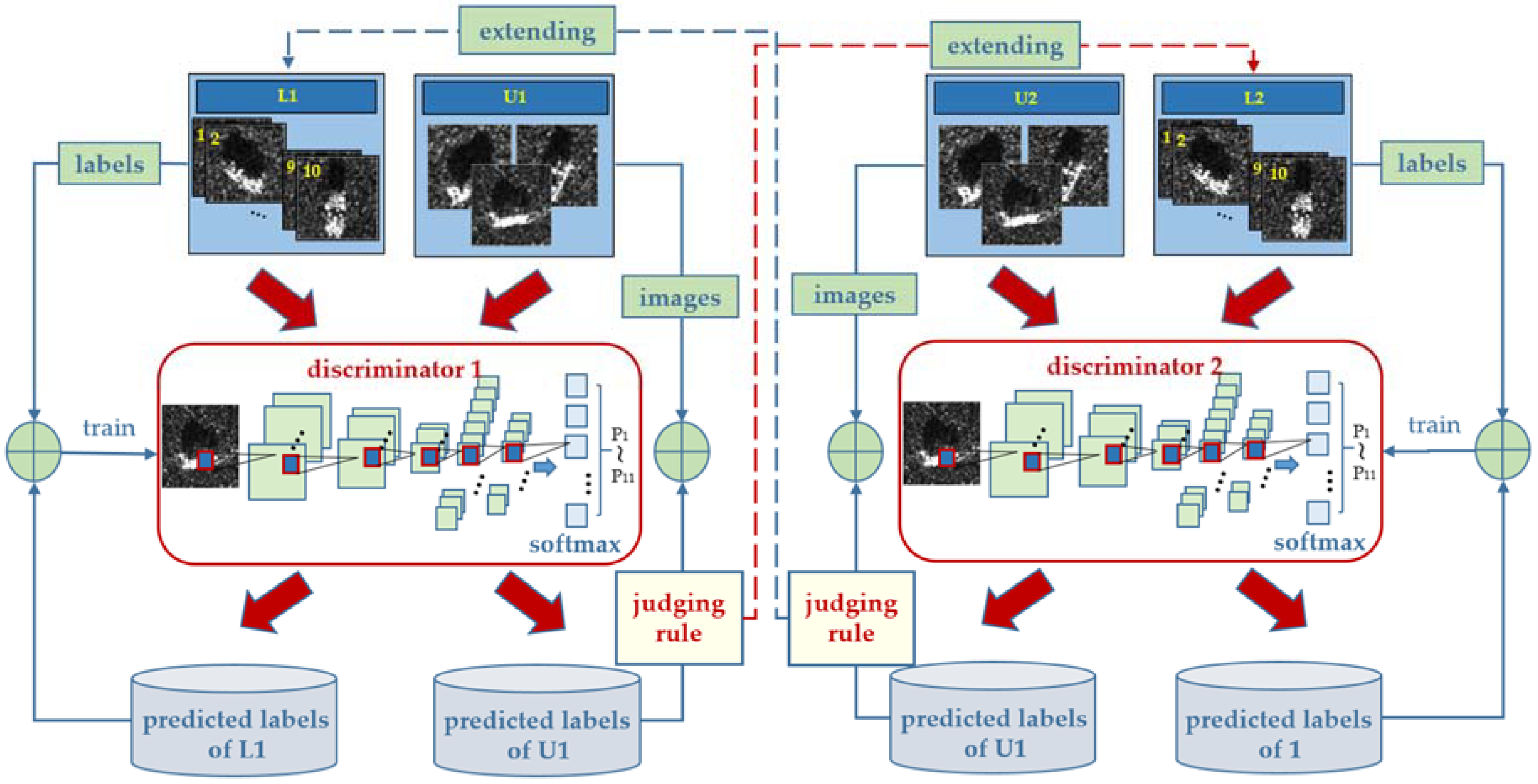As shown in Figure 2, the specific steps of the joint training are as follows:

(1)

utilize $L_1^t$($L_2^t$) to train $D_1^t$($D_2^t$);

(2)

use $D_1^t$($D_2^t$) to predict the labels of the samples in$U_2^t \left( U_1^t\right)$; and,

(3)

$D_1^t$($D_2^t$) selects$p$positive samples from the newly labeled samples according to certain criteria and adds them to $L_2^t$($L_1^t$) for the next round of training.

Note that the newly labeled samples will be regarded as unlabeled samples and will be added to$U$in the next round. Therefore, in each round, all the original unlabeled samples will be labeled, and the selected positive samples are different. As the number of training increases, unlabeled samples will be fully utilized, and the pool of positive samples is increased and diversified. $D_1$and$D_2$are independent from each other in the first two steps. Each time, they select different samples, and they always maintain dynamic differences throughout the process. The difference will gradually decrease after lots of rounds of training and all of the unlabeled samples have been labeled and used to train$D_1$and$D_2$, and the unlabeled samples include the complete features of the unlabeled samples.

A standard is adopted when we select the positive samples. When considering that if the probabilities outputs by the softmax function are very close, then it is not sensible to assign the label with the largest probability to the unlabeled input sample. But, if the maximum probability is much larger than the average of all the remaining probabilities, then it is reasonable to do so. Based on this, we propose a stringent judging rule: if the largest class probability${ P}_{\max }$and the average of all the remaining probabilities satisfy Equation (9), then we can determined that the sample belongs to the class corresponding to${ P}_{\max }$.

$$P_{\max }\ge \alpha \cdot \frac{{\displaystyle \sum _{i=1}^K{P}_i-P_{\max }}}{K-1}$$

(9)

where$K$is the total number of the classes,$\alpha \left(\alpha \ge 1\right)$is a coefficient that measures the difference between${ P}_{\max }$and all of the remaining probabilities. The value$\alpha$is related to the performance of the networks. The better the network performance is, the larger the value of$\alpha$is, and the specific value can be adjusted during the network training.

2.3.2. Noisy Data Learning

In the process of labeling the unlabeled samples, we often meet wrongly labeled samples, which are regarded as noise and will degrade the performance of the network. We look at the application shown in [45], which was based on the noisy data learning theory presented in [47] to reduce the negative effect of the noisy samples. According to the theory, if the labeled sample set$L$has the probably approximate correct (PAC) property, then the sample size$m$satisfies:

$$m=\frac{2\mu }{{\epsilon }^2{\left(1-2\eta \right)}^2}\ln \left(\frac{2N}{\delta }\right)$$

(10)

where$N$is the size of the newly labeled sample set,$\delta$is the confidence,$\mathsf{\epsilon }$is the recognition error rate of the worst hypothetic case,$\eta$is an upper bound of the recognition noise rate, and$\mu$is a hypothetical error that helps the equation be established.

Let$L^t$and$L^{t-1}$denote the samples labeled by the discriminator in the$t$th and the$\left(t-1\right)$th training rounds. The size of sample sets$L\cup L^t$and$L\cup L^{t-1}$are$\left|L\cup L^t\right|$and$\left|L\cup L^{t-1}\right|$, respectively. Let${\eta }_L$denote the noise rate of the original labeled sample set, and$e^t$denotes the prediction error rate. Then, the total recognition noise rate of$L\cup L^t$in the$t$th training round is:

$${\eta }^t=\frac{{\eta }_L\left|L\right|+e^t\left|L^t\right|}{\left|L\cup L^t\right|}$$

(11)

If the discriminator is refined through using$L^t$to train the networks in the$t$th training round, then${\epsilon }^t<{\epsilon }^{t-1}$. In Equation (10), all of the parameters are constant except for$\epsilon$and$\eta$. So, only when${\eta }^t<{\eta }^{t-1},$the equation can still be established. When considering that${\eta }_L$is very small in Equation (11), then${\eta }^t<{\eta }^{t-1}$is bound to be satisfied if$e^t\left|L^t\right|<e^{t-1}\left|L^{t-1}\right|$. Assuming that$0\le e^t,e^{t-1}<0.5$, when$\left|L^t\right|$is far bigger than$\left|L^{t-1}\right|$, we randomly subsample$\left|L^t\right|$whilst guaranteeing$e^t\left|L^t\right|<e^{t-1}\left|L^{t-1}\right|$. It has been proved that if Equation (12) holds, where$s$denotes the size of sample set$\left|L^t\right|$ after subsampling, then$e^t\left|L^t\right|<e^{t-1}\left|L^{t-1}\right|$ is satisfied.

$$s=\lceil \frac{e^{t-1}\left|L^{t-1}\right|}{e^t}-1\rceil$$

(12)

To ensure that$\left|L^t\right|$ is still bigger than$\left|L^{t-1}\right|$after subsampling,$L^{t-1}$should satisfy:

$$\left|L^{t-1}\right|>\frac{e^t}{e^{t-1}-e^t}$$

(13)

Since it is hard to estimate$e^t$on the unlabeled samples, we utilize the labeled samples to compute$e^t$. Assuming that the number of the correctly labeled samples among the total labeled sample set is$n$, then$e^t$can be computed as:

$$e^t=1-\frac{n}{m}$$

(14)

The proposed semi-supervised learning algorithm is presented in Algorithm 1. It should be emphasized that the process of the semi-supervised training is only related to the two discriminators, so the training part of the generator is omitted here.

Algorithm 1. Semi-supervised learning based on multi-output DCGANs.

Inputs: Original labeled training sets $L_1$ and$L_2$, original unlabeled training sets $U_2$ and$U_2$, the prediction sample sets $l_1$ and $l_2$, the discriminators D1 and D2, the error rates $er{r}_1$ and $er{r}_2$, the update flags of the classifiers $updat{e}_1$ and $updat{e}_2$. Outputs: Two vectors of class probabilities $h_1$and$h_2$.

1.  Initialization: for $i=1, 2$ $updat{e}_i\leftarrow True$, $er{r}_i^{\prime }=0.5$, $l_i^{\prime }\leftarrow \varnothing$ 2.  Joint training: Repeat until 400 epoch for $i=1, 2$ (1) If$updat{e}_i=True$, then$L_i\leftarrow L_i\cup l_i^{\prime }$. (2) Use $L_i$ to train $D_i$ and get$h_i$. (3) Allow $D_i$ to label $p_i$ positive samples in U and add them to$l_i$. (4) Allow $D_i$ to measure $er{r}_i$ with$L_i$. (5) If$\left|l_i^{\prime }\right|=0$, then$\left|l_i^{\prime }\right|\leftarrow$ $\lfloor \frac{er{r}_i}{er{r}_i^{\prime } - er{r}_i}+1\rfloor$. (6) If $\left|l_i^{\prime }\right|<\left|l_i\right|$and$er{r}_i\left|l_i\right|<er{r}_i^{\prime }\left|l_i^{\prime }\right|$, then$updat{e}_i\leftarrow True$. (7) If $\left|l_i^{\prime }\right|>$ $\lfloor \frac{er{r}_i}{er{r}_i^{\prime }-er{r}_i}+1\rfloor$, then$l_i\leftarrow Subsample(l_i,$ $\lceil \frac{er{r}_i^{\prime }{l}_i^{\prime }}{er{r}_i}-1\rceil$) and$updat{e}_i\leftarrow True$. (8) If$updat{e}_i=True$, then$er{r}_i^{\prime }\leftarrow er{r}_i, l_i^{\prime }\leftarrow l_i$. 3.  Output:$h_1,h_2.$

3. Experiments and Discussions

3.1. MSTAR Dataset

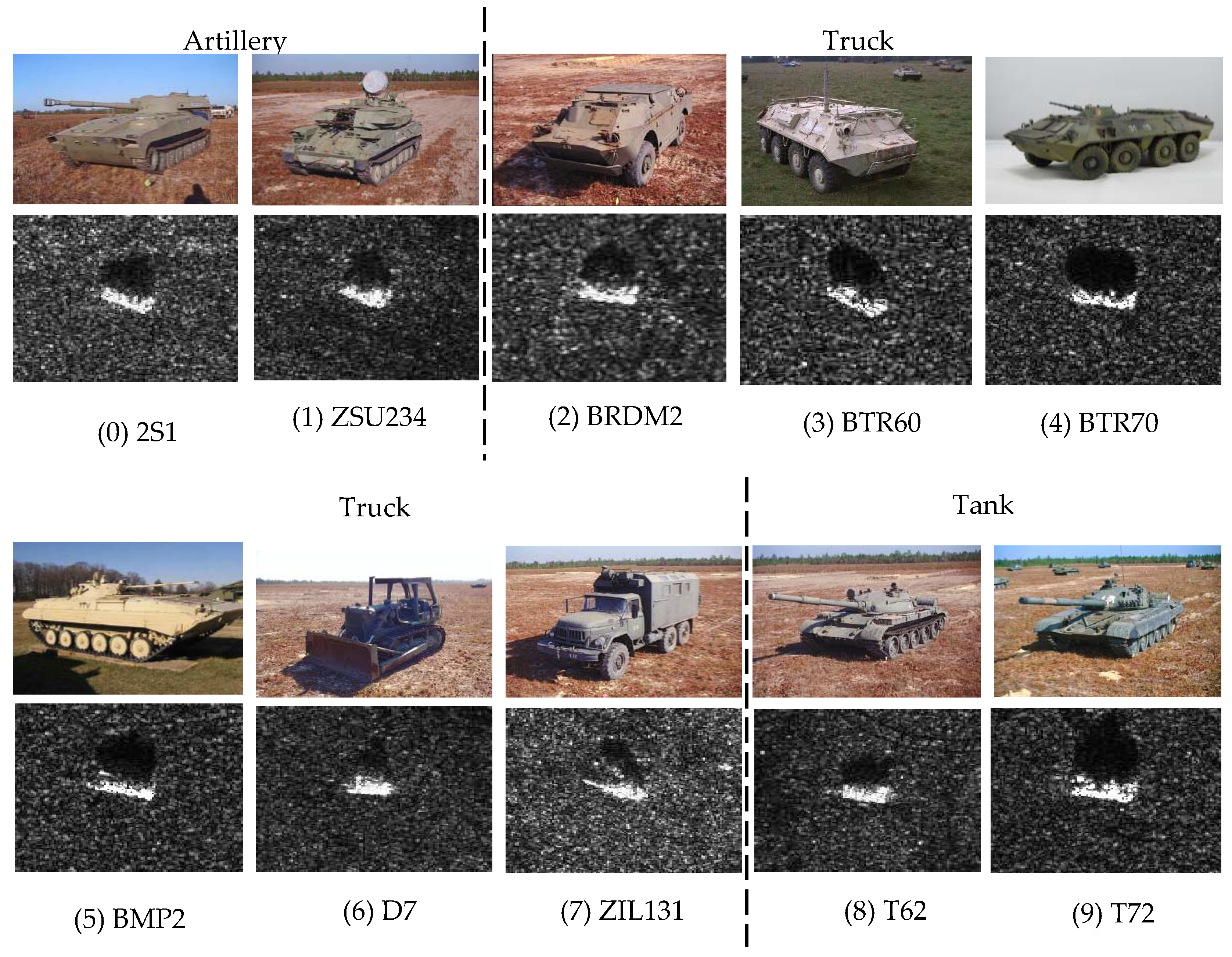
We perform our experiments on the Moving and Stationary Target Acquisition and Recognition (MSTAR) database, which is co-funded by National Defense Research Planning Bureau (ADRPA) and the U.S. Air Force Research Laboratory (AFRL). Ten classes of vehicle objects in the MSTAR database are chosen in our experiments, i.e., 2S1, ZSU234, BMP2, BRDM2, BTR60, BTR70, D7, ZIL131, T62, and T72. The SAR and the corresponding optical images of each class are shown in Figure 3.

3.2. Experiments with Original Training Set under Different Unlabeled Rates

In the first experiment, we partition the original training set that contains 2747 SAR target chips in 17° depression into labeled and unlabeled sample sets under different unlabeled rates, including 20%, 40%, 60%, and 80%. Then, we use the total 2425 SAR target chips in 15° depression for testing. The reason why the training set and the test set take different depressions is that the object features are different in different depressions, which can ensure the generalization ability of our model.

Table 1. Detailed information of the MSRAT dataset used in our experiments.

Tops	Class	Serial No.	Size (Pixels)	Training Set		Testing Set
				Depression	No. Images	Depression	No. Images
Artillery	2S1	B_01	$64\times 64$	$17°$	299	$15°$	274
	ZSU234	D_08	$64\times 64$	$17°$	299	$15°$	274
Truck	BRDM2	E_71	$64\times 64$	$17°$	298	$15°$	274
	BTR60	K10YT_7532	$64\times 64$	$17°$	256	$15°$	195
	BMP2	SN_9563	$64\times 64$	$17°$	233	$15°$	195
	BTR70	C_71	$64\times 64$	$17°$	233	$15°$	196
	D7	92V_13015	$64\times 64$	$17°$	299	$15°$	274
	ZIL131	E_12	$64\times 64$	$17°$	299	$15°$	274
Tank	T62	A_51	$64\times 64$	$17°$	299	$15°$	273
	T72	#A64	$64\times 64$	$17°$	232	$15°$	196
Sum	——	——	——	——	2747	——	2425

lists the detailed information of the target chips that are involved in this experiment, and

Table 2. Specific number of the labeled and unlabeled samples under different unlabeled rates.

Unlabeled Rate	L	U	Total
20%	2197	550	2747
40%	1648	1099	2747
60%	1099	1648	2747
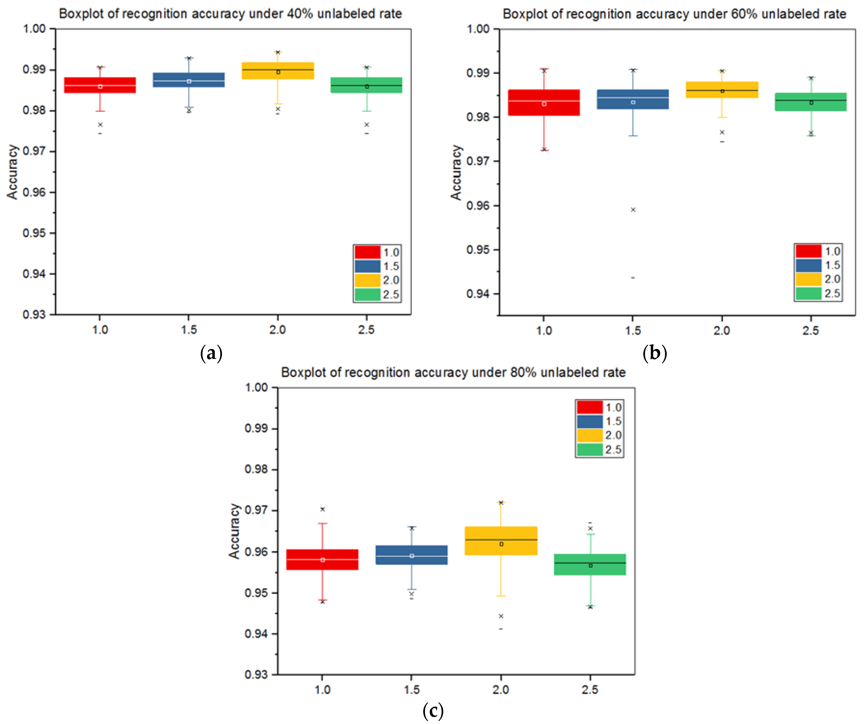
80%	550	2197	2747

lists the specific numbers of the labeled and unlabeled samples under different unlabeled rates. We use L to denote the labeled sample set, U to unlabeled sample set, and NDLT to noisy data learning theory. L+U represents the results obtained by using joint training alone, while L+U+NDLT represents the results that were obtained by using joint training and the noisy data learning theory together. We firstly utilize the labeled samples for supervised training and obtain supervised recognition accuracy (SRA). Then, we simultaneously use the labeled and unlabeled samples for semi-supervised training and obtain semi-supervised recognition accuracy (SSRA). Finally, we calculate the improvement of SSRA over SRA. Both SRA and SSRA are calculated by averaging the 150th to 250th training rounds accuracy of D1 and D2 to reduce accuracy fluctuations. In this experiment, we take $\alpha$ = 2.0 in Equation (9). The experimental results are shown in

Table 3. Recognition accuracy (%) and relative improvements (%) of our semi-supervised learning method under different unlabeled rates. The best accuracies are indicated in bold in each column.

Objects	Unlabeled Rate
	20%					40%
	L	L+U		L+U+NDLT		L	L+U		L+U+NDLT
	SRA	SSRA	imp	SSRA	imp	SRA	SSRA	imp	SSRA	imp
2S1	99.74	99.76	0.02	99.56	−0.18	99.71	99.77	0.07	99.75	0.04
BMP2	97.75	96.62	−1.16	98.07	0.33	97.59	96.65	−0.97	98.36	0.79
BRDM2	96.32	96.04	−0.29	97.13	0.84	94.94	93.04	−2.00	98.61	3.87
BTR60	99.07	98.88	−0.19	98.88	−0.19	98.58	98.70	0.13	99.02	0.45
BTR70	96.31	96.45	0.13	96.40	0.08	94.28	95.27	1.05	97.05	2.93
D7	99.28	98.15	−1.14	99.38	0.10	98.88	98.48	−0.40	99.68	0.81
T62	98.90	99.46	0.57	98.79	−0.11	98.93	99.27	0.34	99.11	0.17
T72	98.53	99.06	0.54	98.93	0.41	97.95	98.40	0.45	99.28	1.35
ZIL131	98.86	97.10	−1.78	98.29	−0.57	97.62	97.20	−0.43	98.84	1.25
ZSU234	99.15	98.92	−0.23	99.45	0.30	98.60	99.49	0.90	99.70	1.11
Average	98.39	98.04	−0.35	98.49	0.10	97.71	97.63	−0.08	98.94	1.26
Objects	Unlabeled Rate
	60%					80%
	L	L+U		L+U+NDLT		L	L+U		L+U+NDLT
	SRA	SSRA	imp	SSRA	imp	SRA	SSRA	imp	SSRA	imp
2S1	99.36	99.69	0.33	99.83	0.47	99.23	99.82	0.59	99.85	0.62
BMP2	95.80	96.18	0.40	97.58	1.85	92.48	95.64	3.42	97.80	5.75
BRDM2	89.01	92.54	3.97	98.40	10.55	75.02	77.26	2.98	83.09	10.76
BTR60	98.67	98.89	0.21	99.20	0.54	95.48	98.02	2.66	98.94	3.62
BTR70	91.27	87.91	−3.69	94.57	3.61	84.94	87.51	3.02	96.78	13.94
D7	97.57	99.27	1.74	99.78	0.26	90.85	90.18	−0.74	98.83	8.79
T62	98.60	99.07	0.48	99.20	0.61	98.16	99.08	0.93	99.07	0.93
T72	95.88	98.84	3.08	99.27	3.53	91.76	94.79	3.30	98.95	7.84
ZIL131	92.75	96.94	4.52	97.96	5.62	86.93	82.41	−5.21	83.78	−3.63
ZSU234	98.63	99.64	1.03	99.67	1.06	97.23	99.72	2.55	99.69	2.53
Average	95.75	96.90	1.19	98.55	2.92	91.21	92.44	1.35	95.68	4.90

.

When comparing the results of L+U and L+U+NDLT, we can conclude that the recognition accuracy is improved after we have introduced the noisy data learning theory. This is because the noisy data will degrade the network performance, and the noisy data learning theory will reduce this negative effect and therefore bring about better recognition results. While comparing the results of L and L+U+NDLT, it can be concluded that the networks will learn more feature information after using the unlabeled samples for training, thus the results of L+U+NDLT is higher than L. We also observe that as the unlabeled rate increases, the average SSRA decreases, while it will obtain higher improvement. It should be noted that the recognition results of the ten classes largely differ. Some classes can achieve high recognition accuracy with only a small number of labeled samples, therefore, the recognition accuracy will not be significantly improved after the unlabeled samples participate in training the networks, such as 2S1, T62, and ZSU234. Their accuracy improvements under different unlabeled rates fall within 3%, but their SRAs and SSRAs are still over 98%. While some classes can obtain large accuracy improvement by utilizing a large number of unlabeled samples for semi-supervised learning, and the more unlabeled samples, the more improvement. Taking BTR70 as an example, its accuracy improvement is 13.94% under an 80% unlabeled rate, but its SRA and SSRA are only 84.94% and 96.78%, respectively.

To directly compare the experimental results, we plot the recognition accuracy curves of L, L+U, and L+U+NDLT corresponding to individual unlabeled ratios, as shown in Figure 4. It is observed that the three curves in Figure 4a look very close, L+U and L+U+NDLT are gradually higher than L in (b,c), and L+U, L+U+NDLT is over L in (d). This indicates that the larger the unlabeled rate is, the more the accuracy improvement can be obtained. Since semi-supervised learning may result in incorrectly labeled samples, which makes it impossible for newly labeled samples to perform, as well as the original labeled samples, the recognition effect will be better with a lower unlabeled rate (simultaneously a higher labeled rate). The experimental result shows that the semi-supervised method that is proposed in this paper is more suitable for those cases when the number of the labeled samples is very small, which is in line with the expectation.

3.3. Quality Evaluation of Generated Samples

One important reason why we adopt DCGANs is that we hope to use the generated unlabeled images for network training in order to improve the performance of our model, when there are only a small number of labeled samples. In this way, we can not only make full use of the existing labeled samples, but also obtain better results than just using the labeled samples for training. We analyze the quality of the generated samples before using them. We randomly select 20%, 30%, and 40% labeled samples (respectively, including 550, 824, and 1099 images) from the original training set for supervised training, then extract images generated in the 50th, 150th, 250th, 350th, and 450th epoch. It should be noted that in this experiment, we want to extract as many high-quality generated images as possible during the training process to improve the network performance. Therefore, we do not limit the number of these high-quality images, then the unlabeled rates cannot be guaranteed to be 40%, 60%, and 80%, respectively. 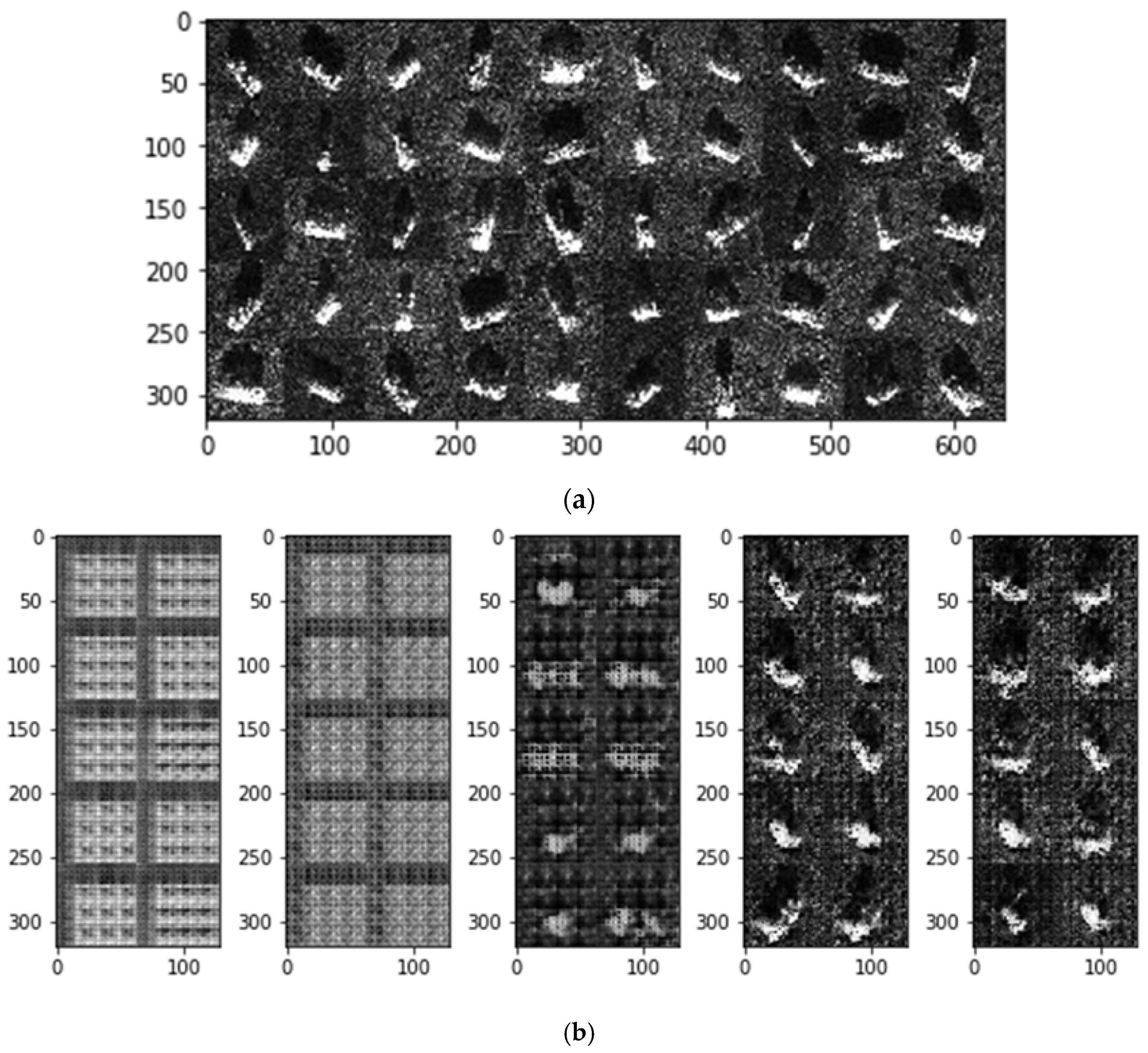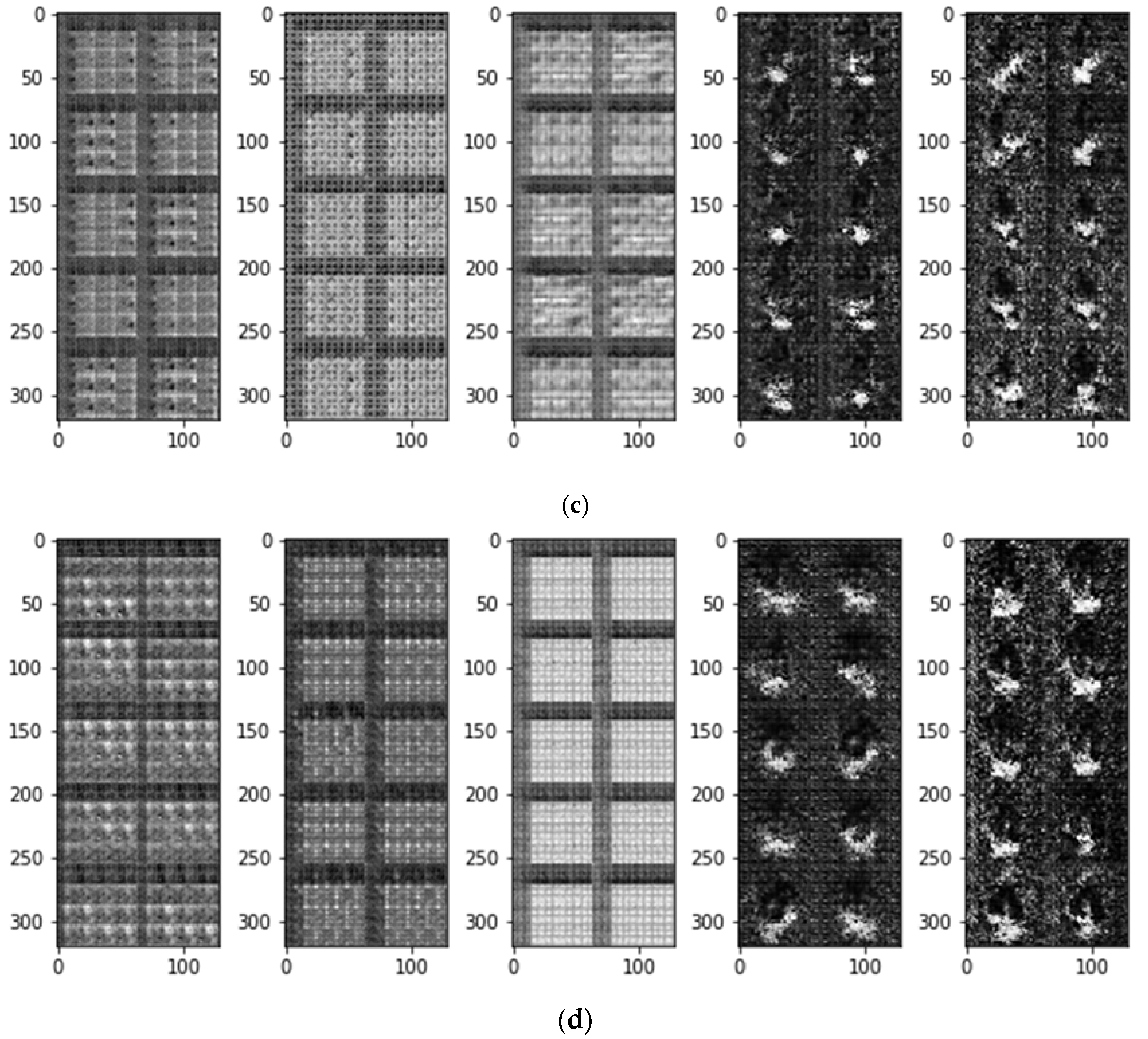Figure 5a shows the original SAR images, and (b–d) show the images generated with 1099, 824, and 550 labeled samples, respectively. In (b,c), each group of images from left to right is generated in the 50th, 150th, 250th, 350th, and 450th epoch.

We can see that as the training epoch increases, the quality of the generated images gradually becomes higher. In Figure 5b, objects in the generated images are already roughly outlined in the 250th epoch, and the generated images are very similar to the original images in the 350th epoch. In Figure 5c, objects in the generated images are clear until the 450th epoch is taken. In Figure 5c, the quality of the generated images is still poor in the 450th epoch.

In order to confirm the observations that are described above, we select 1000 images from each group of the generated images shown in Figure 5b–d and, respectively, input them into a well-trained discriminator, then count the total number of the samples that satisfy the rule shown in Equation (9), as presented in Section 2.3.1. We still use α = 2.0 in this formula. We believe that those samples which satisfy the rule are of high quality and can be used to train the model. The results listed in

Table 4. The number of high-quality samples in 1000 generated samples from the 50th, 150th, 250th, 350th, and 450th epoch with different numbers of labeled samples.

Epoch	The Number of Labeled Samples
	1099	824	550
50	0	0	0
150	0	0	0
250	23	0	0
350	945	44	76
450	969	874	551

are consistent with what we expect.

3.4. Experiments with Unlabeled Generated Samples under Different Unlabeled Rates

This experiment will verify the impact of the high-quality generated images on the performance of our model. We have confirmed in Section 3.2 that the semi-supervised recognition method that is proposed in this paper leads to satisfactory results in the case of a small number of labeled samples. Therefore, this experiment will be related to this case. The labeled samples in this experiment are selected from the original training set, and the generated images are used as the unlabeled samples. The testing set is unchanged. According to the conclusions made in Section 3.3, we select 1099, 824, 550 labeled samples from the original training set for supervised training, then, respectively, extract those high-quality generated samples in the 350th, 450th, and 550th epoch, and utilize them for semi-supervised training. It should be emphasized that since the number of the selected high-quality images is uncertain, the total amount of the labeled and unlabeled samples no longer remains at 2747. The experimental results are shown in

Table 5. Recognition accuracy (%) and relative improvements (%) obtained with our semi-supervised learning method with different number of original labeled samples. The best accuracies are indicated in bold in each column.

Objects	The Number of Original Labeled Samples
	1099			824			550
	SRA	SSRA	imp	SRA	SSRA	imp	SRA	SSRA	imp
2S1	99.54	99.94	0.19	99.31	99.71	0.40	99.06	99.82	0.76
BMP2	94.60	95.14	0.58	95.36	96.78	1.49	92.57	90.35	−2.39
BRDM2	93.07	88.67	−4.72	87.67	91.17	4.00	74.66	85.51	14.52
BTR60	99.11	98.57	−0.55	98.19	98.11	−0.07	95.95	97.16	1.26
BTR70	91.95	95.84	4.23	88.57	91.25	3.02	85.48	86.67	1.39
D7	99.18	99.78	0.60	96.36	98.72	2.45	91.68	96.48	5.23
T62	98.53	99.00	0.48	99.14	99.21	0.07	98.64	98.26	−0.39
T72	97.61	98.28	0.69	95.73	95.51	−0.23	90.67	94.33	4.05
ZIL131	95.43	94.04	−1.46	91.23	93.68	2.68	87.62	85.21	−2.74
ZSU234	98.71	98.53	−0.18	98.65	98.65	0.00	97.25	98.21	0.99
Average	96.77	96.76	0.00	95.02	96.28	1.33	91.36	93.20	2.01

.

It can be found that the average SSRA will obtain better improvement with less labeled samples. Different objects vary greatly in accuracy improvement. The generated samples of some types can provide more feature information, so our model will perform better after using these samples for training, and the recognition accuracy will also be improved significantly, such as BRDM2 and D7. Their accuracy improvements will significantly increase as the number of the labeled samples decreases. Note that BRDM2 performs worse with 1099 labeled samples, but much better with 550 labeled samples. This is because the quality of the generated images is much worse than that of the real image, therefore, the generated images will make the recognition worse when there is a large number of labeled samples. When the number of the labeled samples is too small, using a large number of generated samples can effectively improve the SSRA, but the SSRA cannot exceed the SRA of a little more labeled samples, such as the SRA of 824 and 1099 labeled samples. However, the generated samples of some types become worse as the number of the labeled samples decrease, and thus the improvement tends to be smaller, such as BTR70. Meanwhile, some generated samples are not suitable for network training, such as ZIL131. Its accuracy is reduced after the generated samples participate in the training, and we believe that the overall accuracy will be improved by removing these generated images.

We have found that when the number of the labeled samples is less than 500, there is almost no high-quality generated samples. Therefore, we will not consider using the generated samples for training in this case.

3.5. Comparison Experiment with Other Methods

In this part, we compare the performance of our method with several other semi-supervised learning methods, including label propagation (LP) [50], progressive semi-supervised SVM with diversity P${\mathrm{S}}^3$VM-D [42], Triple-GAN [51], and improved-GAN [49]. LP establishes a similar matrix and propagates the labels of the labeled samples to the unlabeled samples, according to the degree of similarity. P${\mathrm{S}}^3$VM-D selects the reliable unlabeled samples to extend the original labeled training set. Triple-GAN consists of a generator, a discriminator, and a classifier, whilst the generator and the classifier characterize the conditional distributions between images and labels, and the discriminator solely focuses on identifying fake images-label pairs. Improved-GAN adjusts the network structure of GANs, which enables the discriminator to recognize multiple object types.

Table 6. Recognition accuracy (%) of LP, P${\mathrm{S}}^3$VM-D, Triple-GAN, Improved-GAN, and our method with different unlabeled rates.

Method	Unlabeled Rate
	20%	40%	60%	80%
LP	96.05	95.97	94.11	92.04
P$S^3$VM-D	96.11	96.02	95.67	95.01
Triple-GAN	96.46	96.13	95.97	95.70
Improved-GAN	98.07	97.26	95.02	87.52
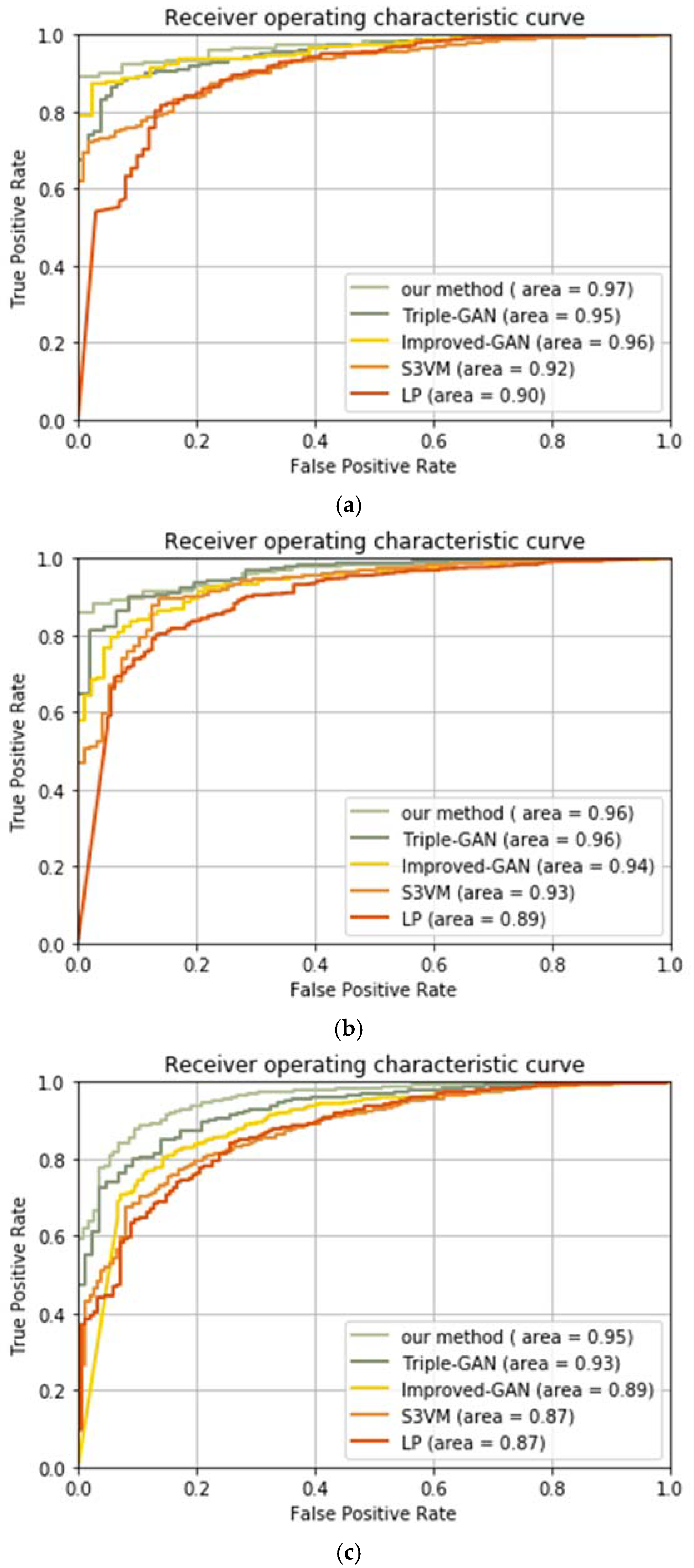
Our Method	98.14	97.97	97.22	95.72

lists the accuracies of each method under different unlabeled rates.

We can conclude from Table 6 that our method performs better than the other methods. There are mainly two reasons for this: one is that CNNs is used as the classifier in our model, which can extract more abundant features than the traditional machine learning methods, such as LP and P${\mathrm{S}}^3$VM-D, also other GANs that consist of no CNNs, such as Triple-GAN and improved-GAN; the other is that we have introduced the noisy data learning theory, and it has been proved that the negative effect of noisy data can be reduced with this theory, and therefore bring better recognition results. It can be found that as the unlabeled rate increases, the system performance becomes worse. Especially when the unlabeled rate increases to 80%, the recognition accuracy of LP and Improved-GAN decreases to 73.17% and 87.52%, respectively, meaning that these two methods cannot cope with the situations where there are few labeled samples. While P${\mathrm{S}}^3$VM-D, Triple-GAN, and our method can achieve high recognition accuracy with a small number of labeled samples, and our method has the best performance with individual unlabeled rates. In practical applications, label samples are often difficult to obtain, so a good semi-supervised method should be able to use a small number of labeled samples to obtain high recognition accuracy. In this sense, our method is promising.

4. Discussion

4.1. Choice of Parameter$\alpha$

In this section, we will further discuss the choice of parameter$\alpha$. The value of$\alpha$will place restrictions on the confidence of the predicted labels of the unlabeled samples, and the larger the value of$\alpha$, the higher the confidence. When using the generated images as the unlabeled samples, we can select those generated images of higher quality for the network training by taking a larger value for$\alpha$. Therefore, the value of$\alpha$plays an important role in our method. According to the experimental results that are shown in Section 3.2, when the unlabeled rate is small, such as 20%, unlabeled samples have little impact on the performance of the model. So, in this section, we only analyze the impact of$\alpha$on the experimental results when the unlabeled rates are 40%, 60%, and 80%. We determine the possibly best value of$\alpha$by one-way analysis of variance (one-way ANOVA). With different unlabeled rates, we specify the values 1.0, 1.5, 2.0, 2.5, 3.0 for$\alpha$, and perform five sets of experiments, and 100 rounds of training per set.

The ANOVA table is shown in

Table 7. ANOVA table under different unlabeled rates.

Unlabeled Rate	Source	SS	df	MS	F	Prob > F
40%	Intergroup	0.00081	3	0.00027	33.62	$2.23\times {10}^{-19}$
	Intragroup	0.00316	396	0.00001	-	-
	Total	0.00397	399	-	-	-
60%	Intergroup	0.00055	3	0.00018	11.80	$2.03\times {10}^{-7}$
	Intragroup	0.00619	396	0.00002	-	-
	Total	0.00674	399	-	-	-
80%	Intergroup	0.00149	3	0.00050	27.11	$5.76\times {10}^{-16}$
	Intragroup	0.00726	396	0.00002	-	-
	Total	0.00875	399	-	-	-

. It should be noted that almost no unlabeled samples can be selected for training when$\alpha =3$, so we finally give up the corresponding experimental data. Columns 2 to 6 in Table 7 refer to the source of the difference (intragroup or intergroup), sum squared deviations (SS), degree of freedom (df), mean squared deviations (MS), F-Statistic (F), and detection probability (Prob > F). It can be seen from Table 7 that intergroup MS is far greater than intragroup MS, indicating that the intragroup difference is small, while the intergroup difference is large. Meanwhile, F is much larger than 1 and Prob is much less than 0.05, which also supports that the intergroup difference is significant. Intergroup difference is caused by different values of$\alpha$. We can conclude that the value of$\alpha$has great influence on the experimental results.

To directly compare the experimental results of different values of$\alpha$, we draw boxplots of recognition accuracy with different unlabeled rates, as shown in Figure 6. We use red, blue, yellow, and green boxes to represent the recognition results when$\alpha$is 1.0, 1.5, 2.0, and 2.5, respectively. It can be found from Figure 6 that the yellow box’s median line is higher than the rest of the boxes at individual unlabeled rates, showing that the average level of recognition accuracy is higher when$\alpha =2$. This is because, when the value of$\alpha$is small, the confidence of the labels is not guaranteed, and there may be more wrongly labeled samples involved in the training; when the value is large, only a small number of high-quality samples can be selected for the training and the unlabeled samples are not fully utilized. In Figure 6a,b, the yellow boxes have smaller widths and heights, which indicates more concentrated experimental data and more stable experimental process. In Figure 6c, the width and height of the yellow box are bigger. Therefore, we chose$\alpha =2$with different unlabeled rates to obtain satisfactory recognition results.

4.2. Performance Evaluation

4.2.1. ROC Curve

We have compared the recognition results of different methods on the MSTAR database. However, the comparison results cannot explain the generalization capability of our method on different datasets. In this section, we will compare the performance of different methods through the receiver operating characteristic (ROC) curves [52]. As shown in Section 4.1, we let$\alpha =2$, and plot the ROC curves of these methods with the unlabeled rate 40%, 60%, 80%, as shown in Figure 7.

It can be found that our method achieves better performance when compared with the other methods. In Figure 7a–c, the areas under the ROC curves of our method are close to 1, and the TPR values are greater than 0.8, while keeping low FPR. The areas under the ROC curves of the other methods are smaller than our method. We can learn from Figure 7 that, as the unlabeled rate decreases, the area of ROC curves of these methods decreases, and the smaller the unlabeled rate, the better performance of our method. The experimental results confirm that our method has a better generalization capability.

4.2.2. Training Time

In our method, after each round of training, those newly labeled samples with high label confidence will be selected for the next round. The network performance varies under different unlabeled rates, thus the total number of the selected newly labeled samples is different. Therefore, the time for each round of training is also different. In this section, we will analyze the training time of the proposed method [53]. We calculate the average training time from the 200th epoch to the 400th epoch at different unlabeled rates. The main configuration of the computer is: GPU: Tesla K20c; 705 MHz; 5 GB RAM; operating system: Ubuntu 16.04; running software: Python 2.7. The calculation results are shown in

Table 8. Training time under different unlabeled rates.

Unlabeled Rate	Training Time (Sec/Epoch)	Total Epochs
20%	40.71	200
40%	40.21	200
60%	39.79	200
80%	38.80	200

.

It can be found that, as the unlabeled rates increase, the training time tends to decrease. This is because when the unlabeled rate is larger, the original labeled samples are less; however, the network performs better with more original labeled samples, and more newly labeled samples can thus be selected, resulting in time increment. The conclusion is consistent with the previous analysis.

5. Conclusions

In this study, we presented a DCGANs-based semi-supervised learning framework for SAR automatic target recognition. In this framework, we doubled the discriminator of DCGANs and utilized the two discriminators for semi-supervised joint training. The last layer of the discriminator is replaced by a softmax function, and its loss function is also adjusted accordingly. Experiments on the MSTAR dataset have led to the following conclusions:

• Introducing the noisy data learning theory into our method can reduce the adverse effect of the wrongly labeled sample on the network and significantly improve the recognition accuracy.
• Our method can achieve high recognition accuracy on the MSTAR dataset, and especially performs well when there are a small number of labeled samples and a large number of unlabeled samples. When the unlabeled rate increases from 20% to 80%, the overall accuracy improvement increases from 0 to 5%, and the overall recognition accuracies are over 95%.
• The experimental results have confirmed that when the number of the labeled samples is small, our model performs better after utilizing those high-quality generated images for the network training. The less the labeled samples, the higher the accuracy improvement. However, when the labeled samples are less than 500, the quality of the generated samples are too few to make the system work.