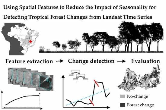
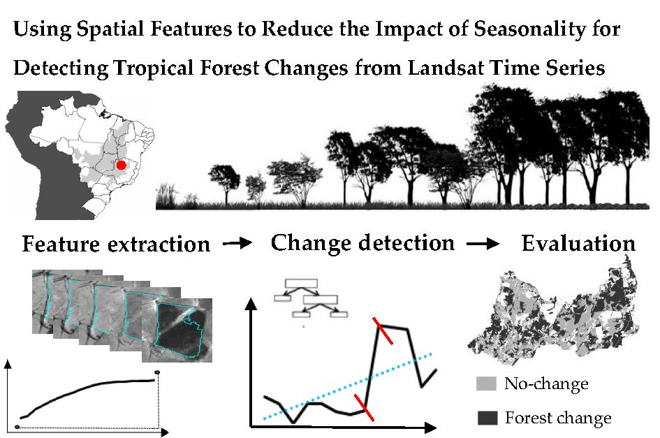
Using Spatial Features to Reduce the Impact of Seasonality for Detecting Tropical Forest Changes from Landsat Time Series

 , , ,
, , ,
Abstract
:
1. Introduction
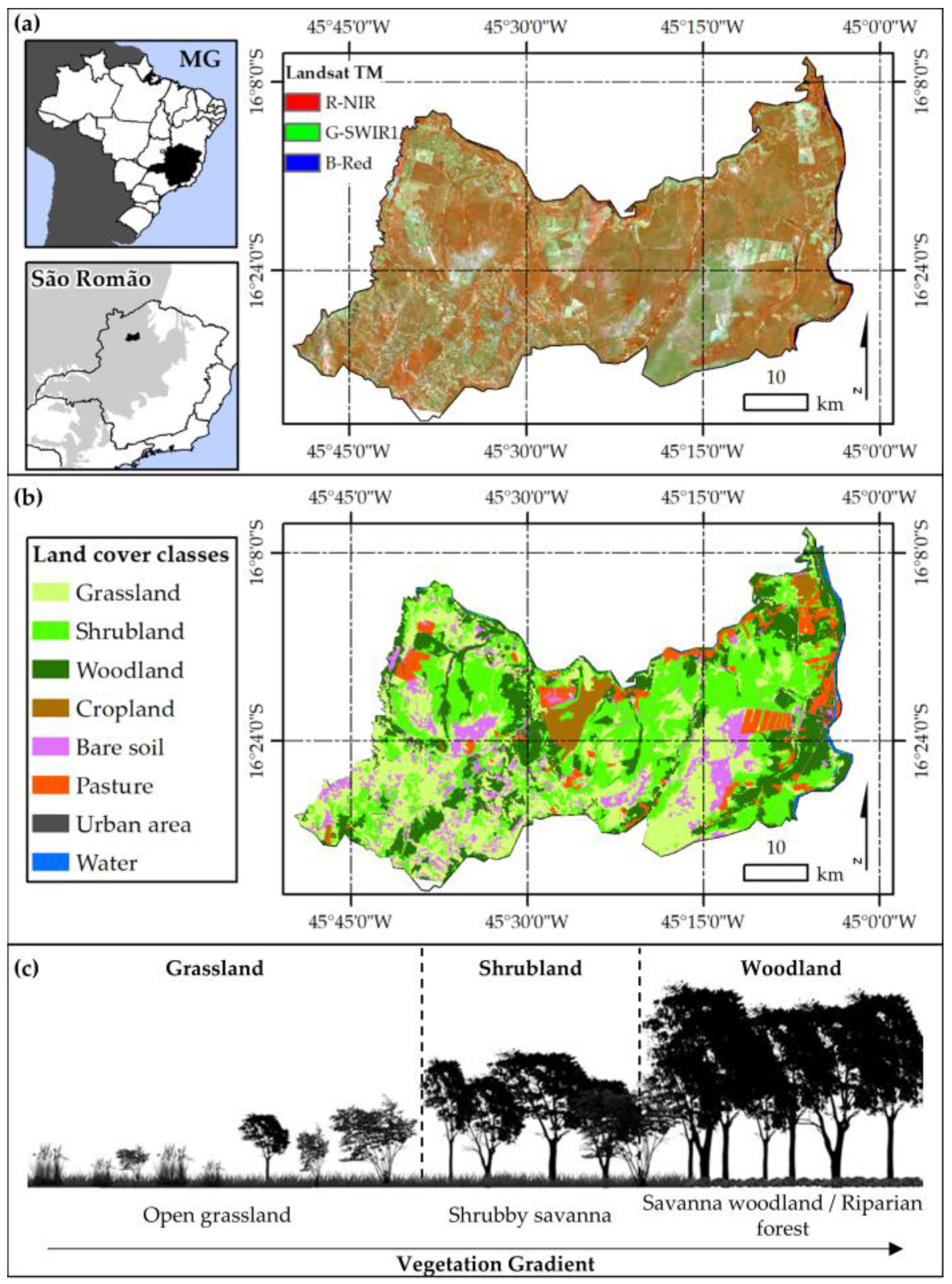
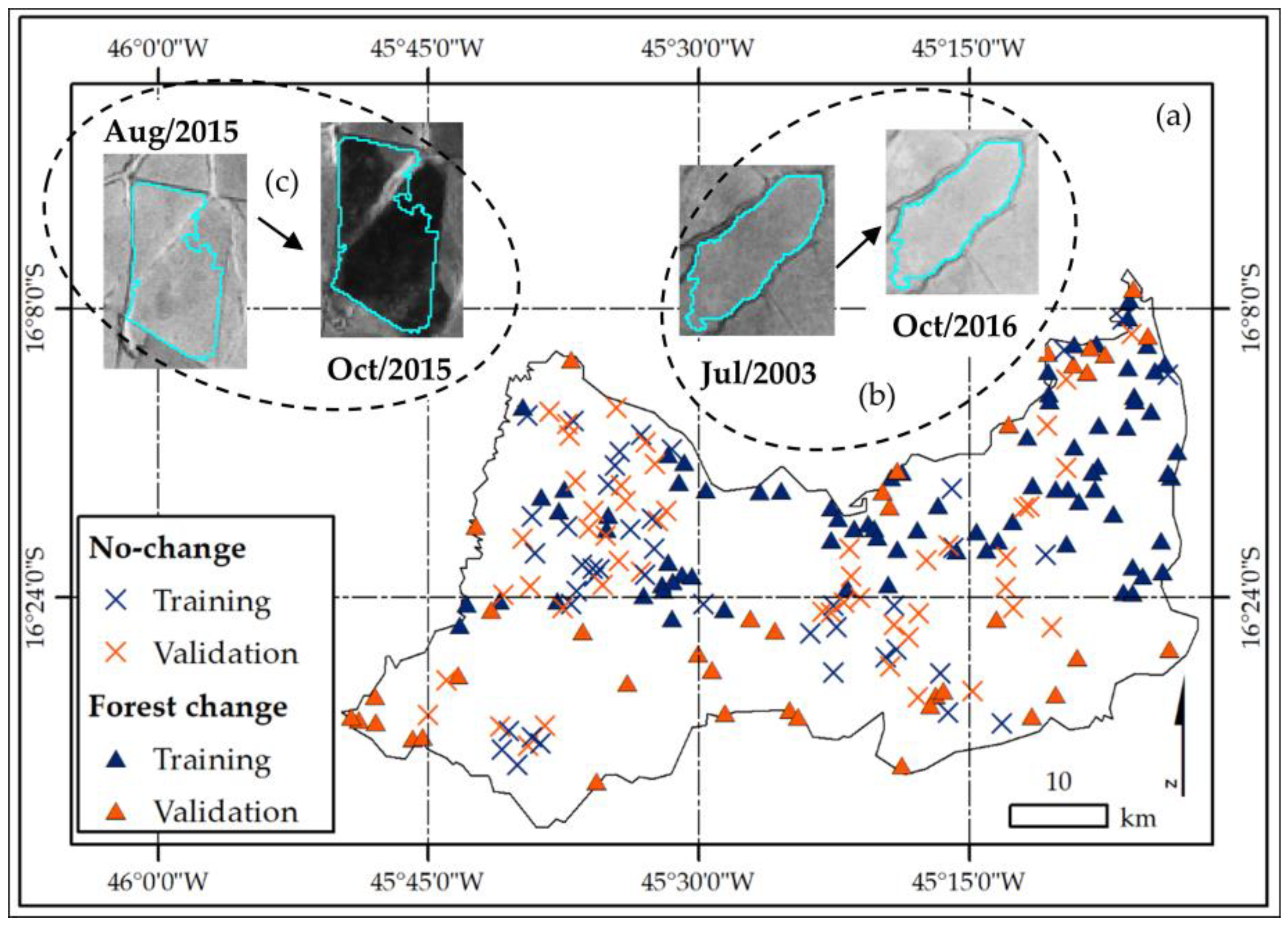
2. Study Area
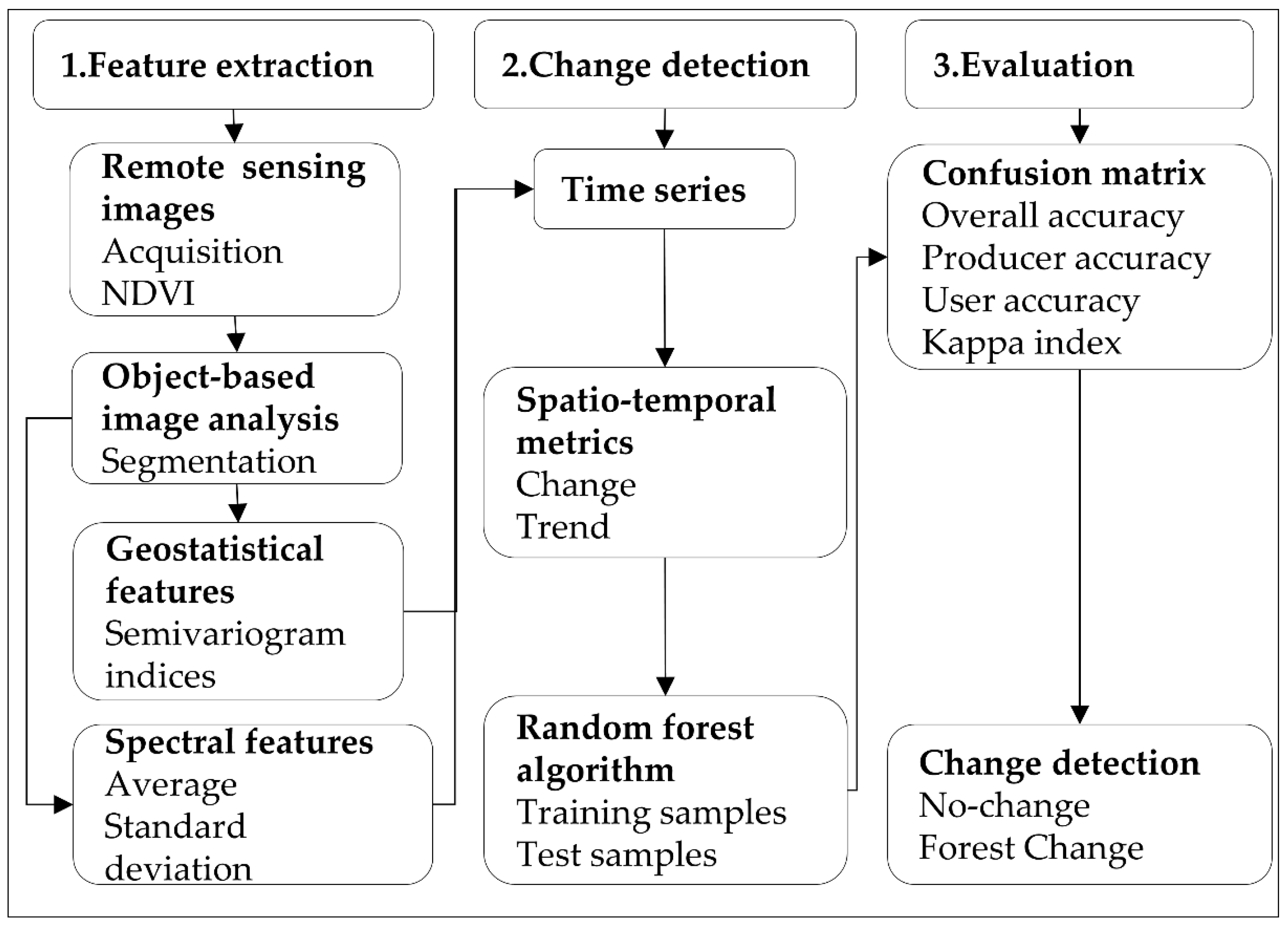
3. Methodology
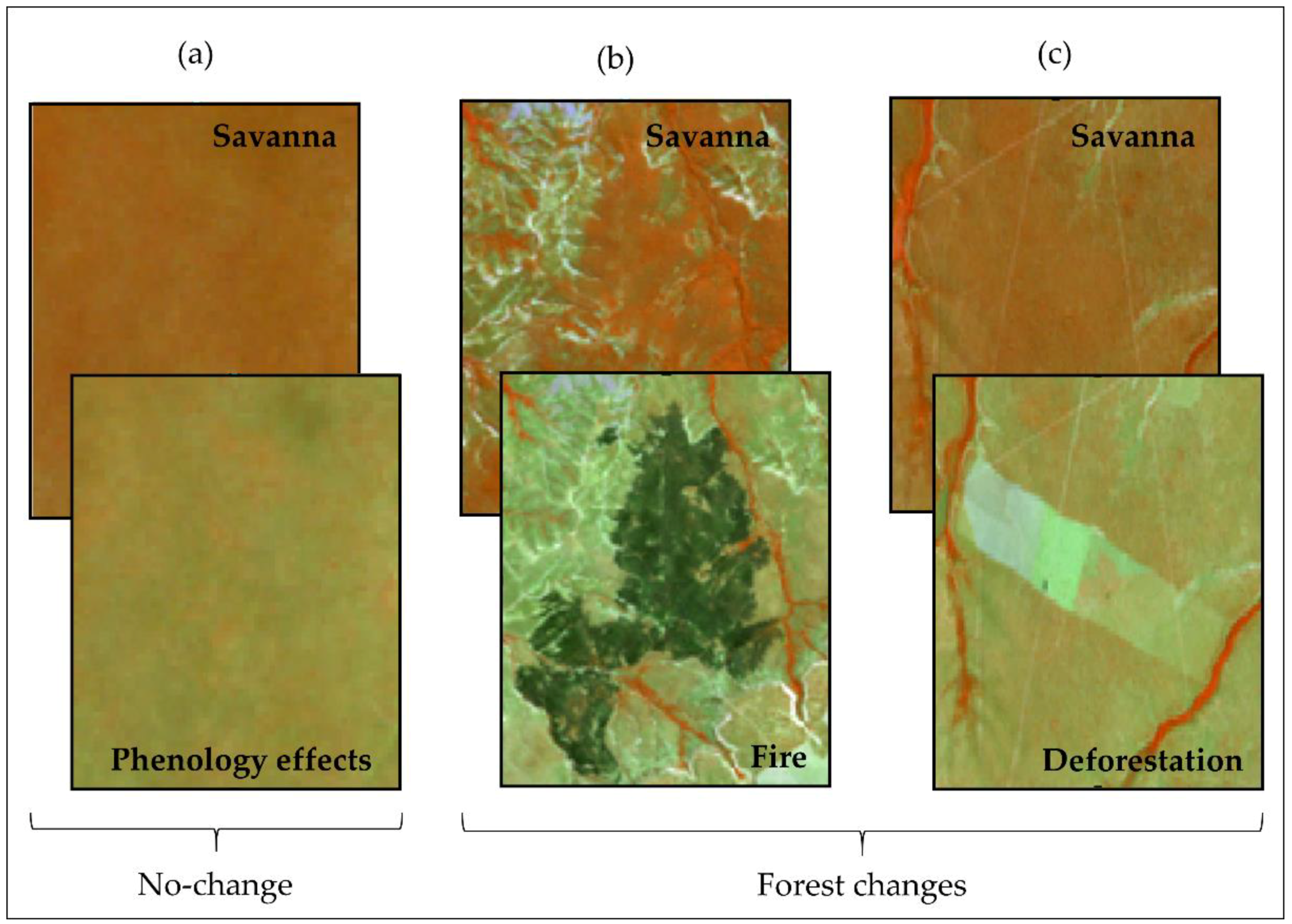
- No-change: seasonal changes due to phenological effects (natural events)
- Forest change: land cover changes such as deforestation (human-induced) and fires (both natural events and human induces)
3.1. Satellite Data and Processing
3.2. Object-Based Image Analysis
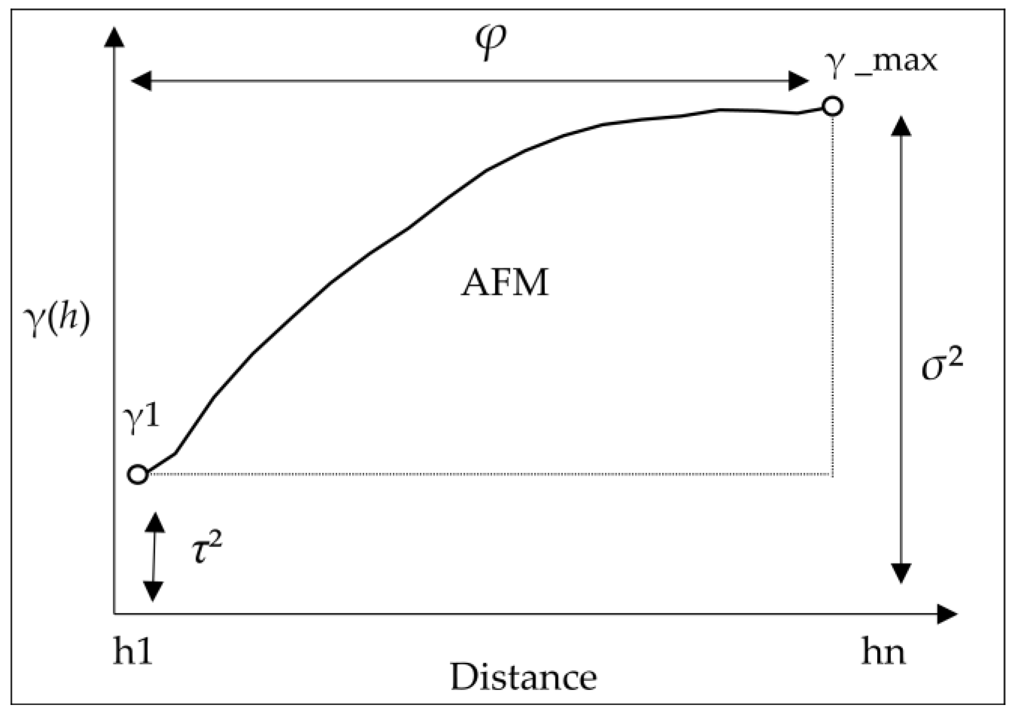
3.3. Geostatistical and Spectral Features
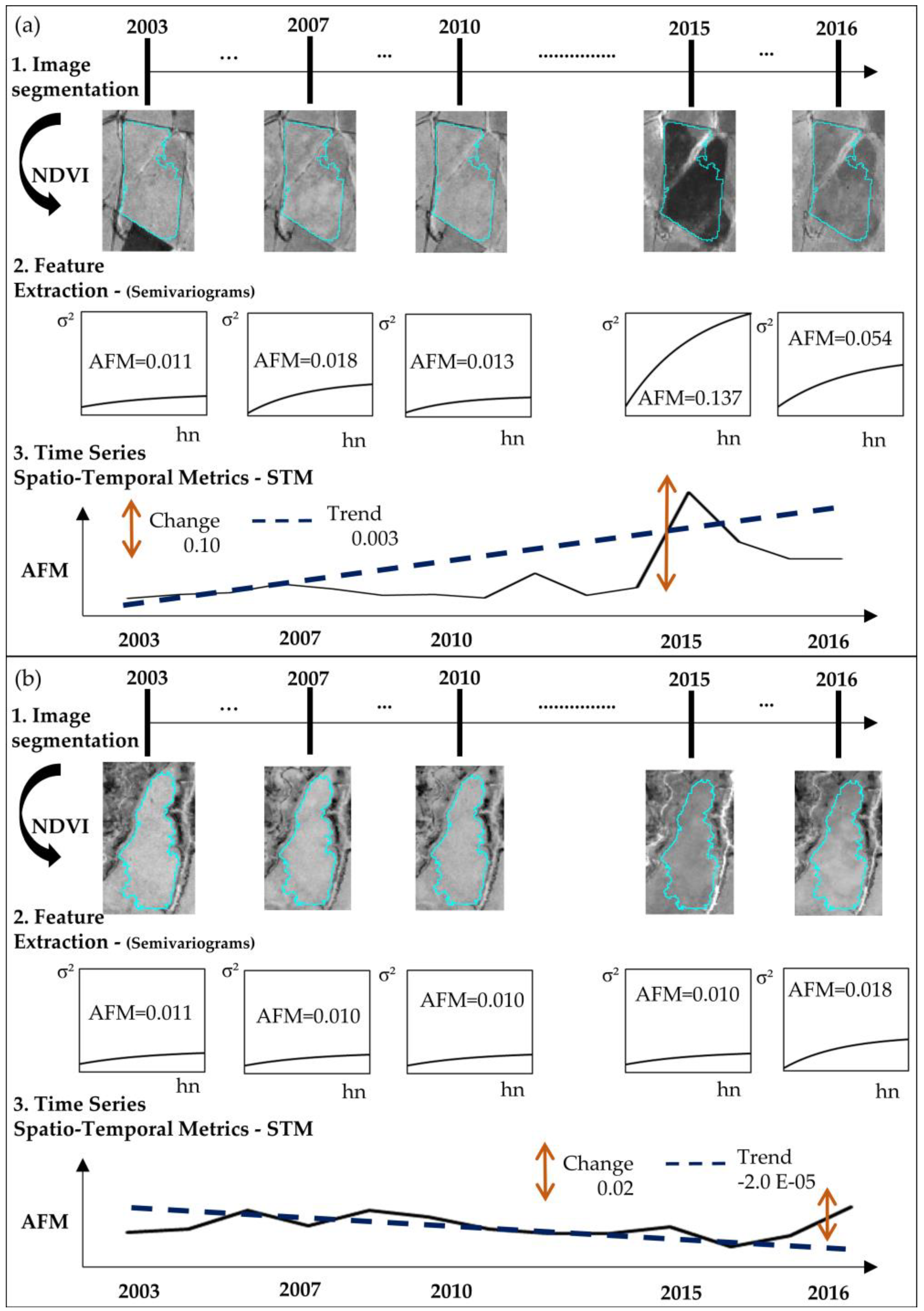
3.4. Time Series
3.5. Spatio-Temporal Metrics (STM)
3.6. Random Forest Algorithm
3.7. Change Detection Evaluation
4. Results
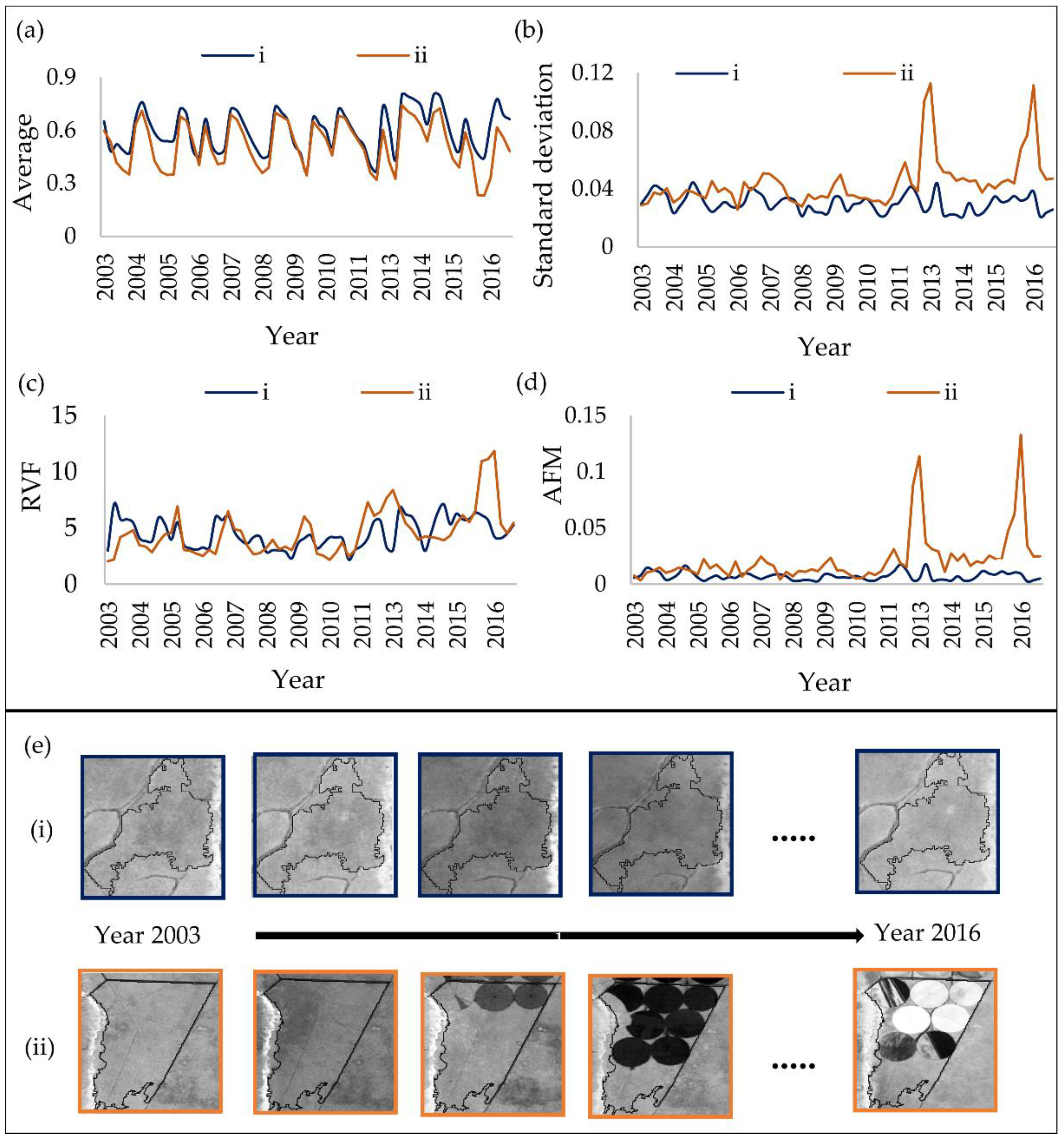
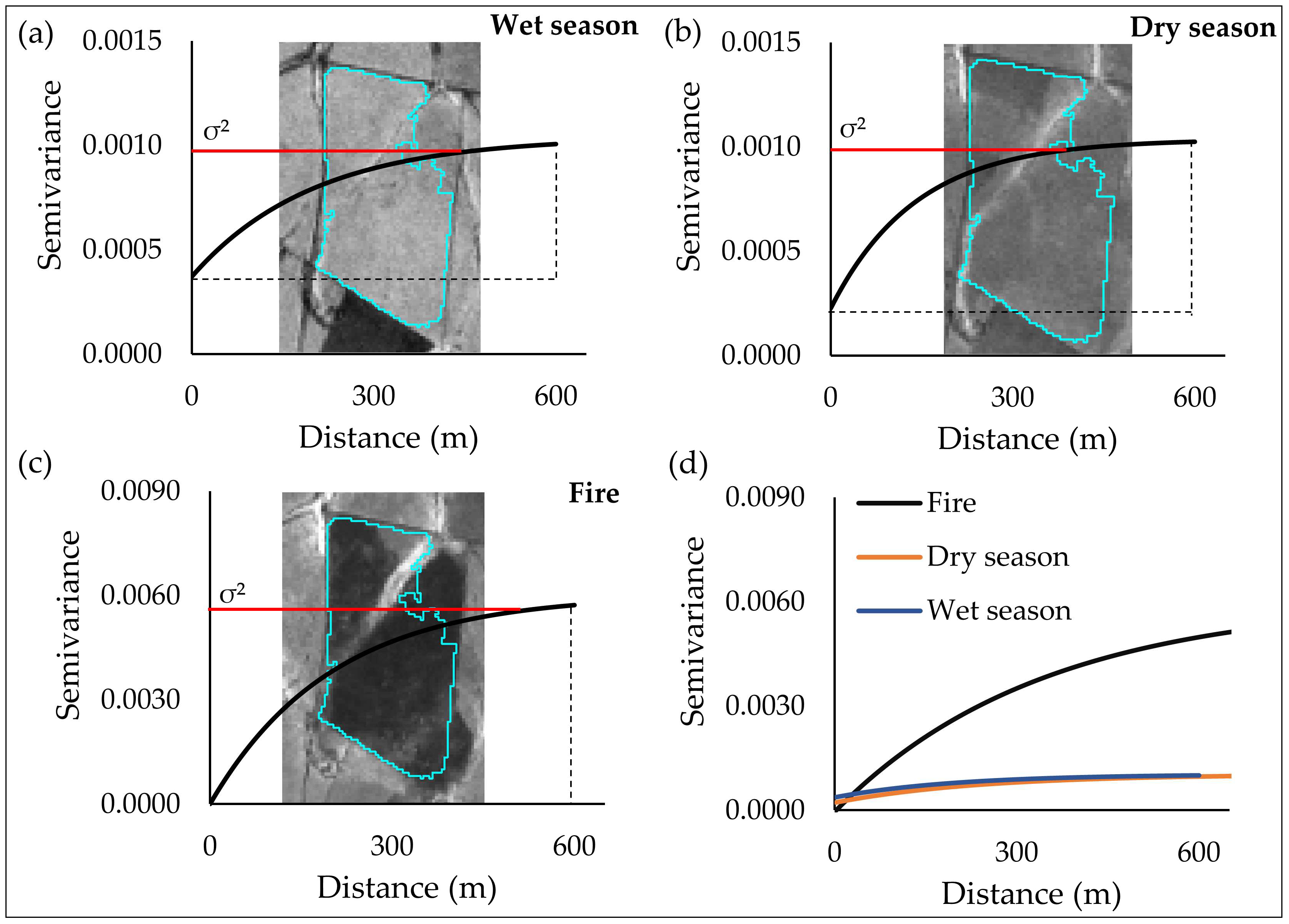
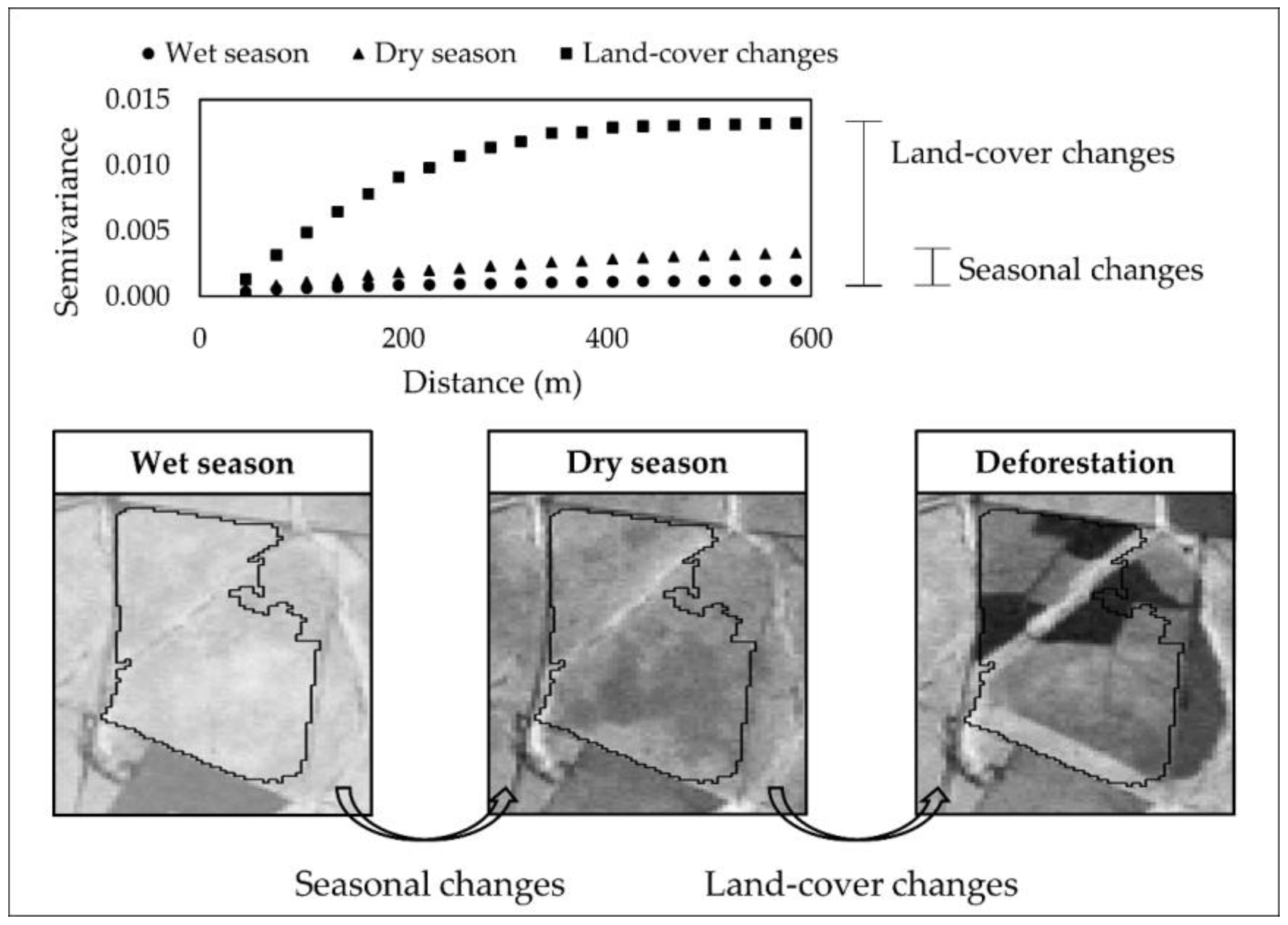
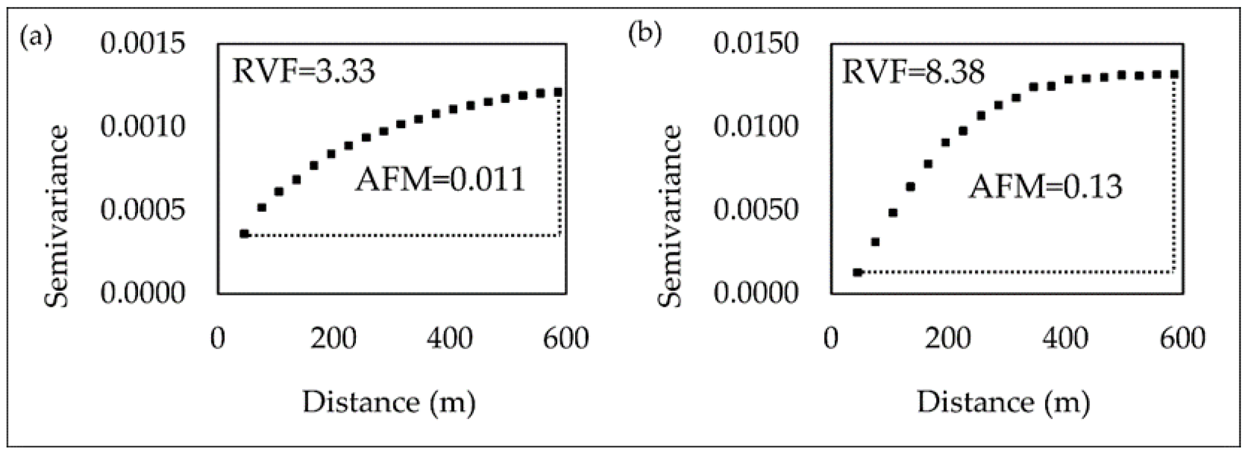
4.1. Semivariogram Analysis
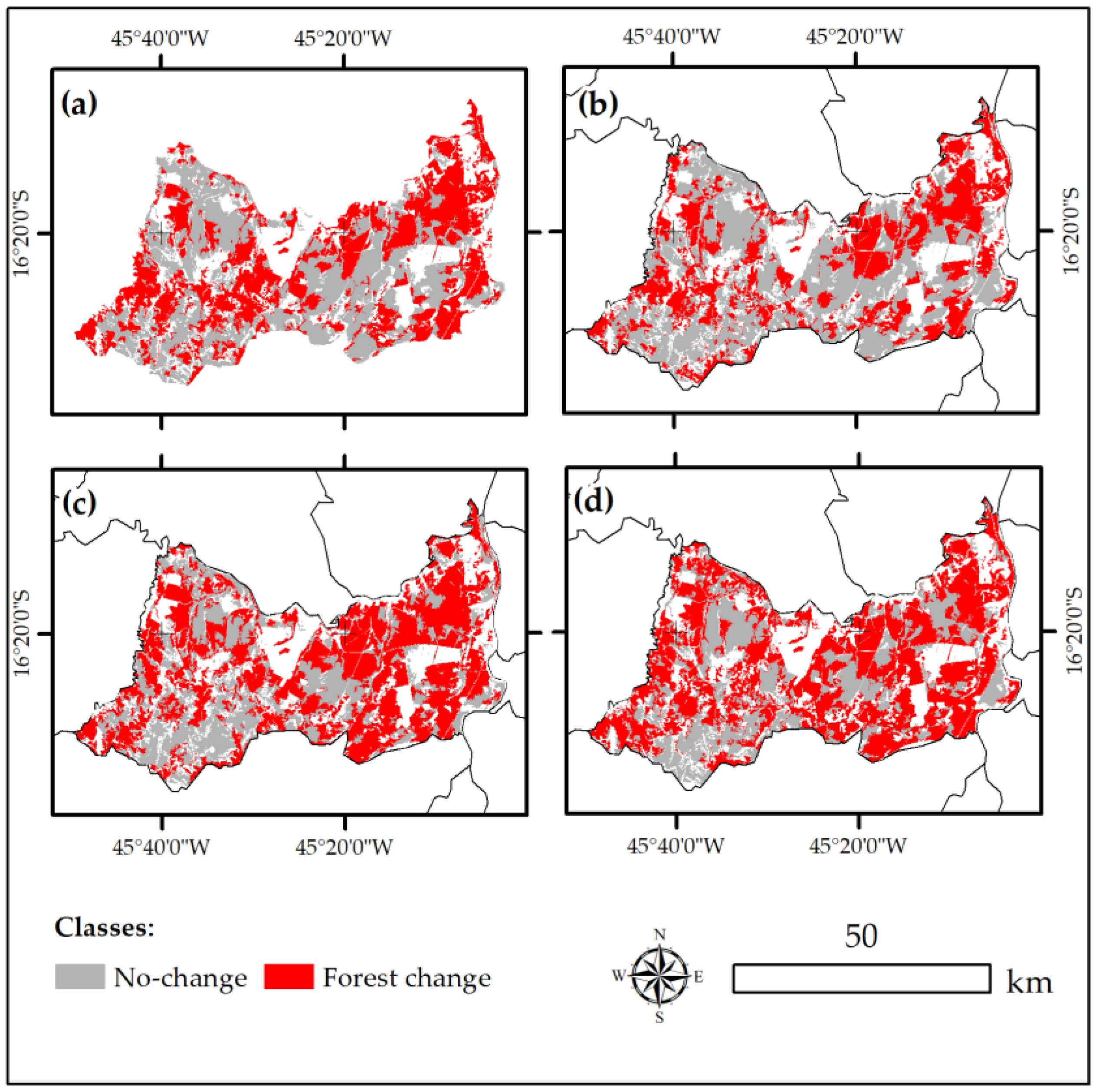
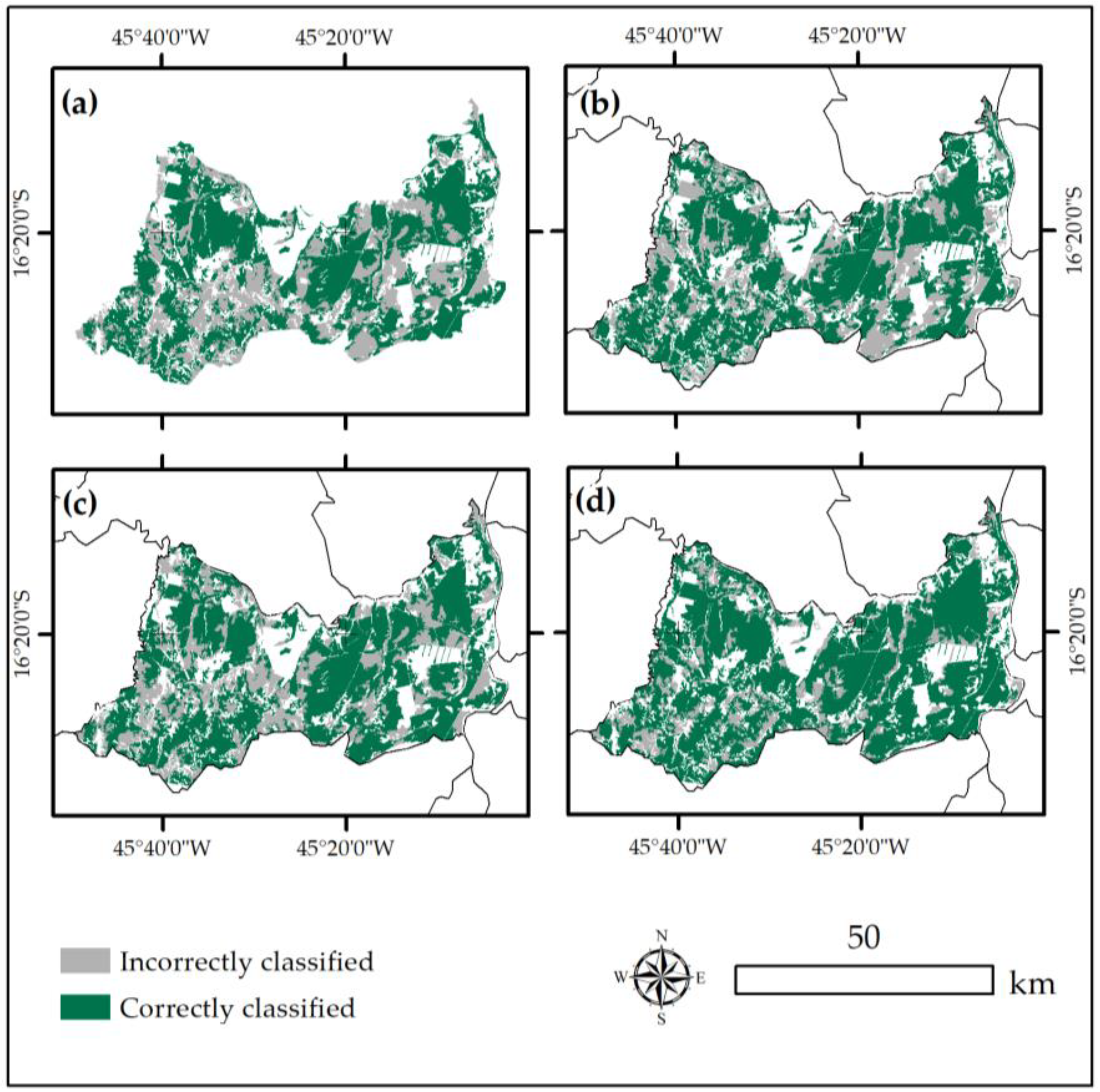
4.2. Change Detection
5. Discussion
5.1. NDVI Spatial Variability
5.2. Seasonal Effects on Change Detection
5.3. Method Limitations
- (1)
- Forest change quantification: The method can identify the objects undergoing land cover changes without being impacted by seasonal variations; however, it is not possible to accurately calculate the changed area. Due to use of an object-based approach, some changes do not cover the entire object because the forest change class comprised both small changes reaching up to 20% of the objects and large changes ranging from 50% to 100% of the object area. This limitation is related to the initial image segmentation performed on the first image of the time series (image object overlay) rather than segmenting the entire time series (multitemporal image object). We used this technique because it provides a more meaningful framework for spatial measures [51], capable of capturing the intra-object heterogeneity [74]. Further research into how the proportion of pixels changed inside the objects (real area of forest change) affect the resultant accuracies remain outstanding.
- (2)
- Timing of changes: The method allows for the discrimination between forest change and no-change classes, however, it is not possible to indicate when exactly the forest changes have occurred. Although the timing of the change is an important feature of forest monitoring, we did not attempt to model the time of the change, as our main focus is not hinged on the capacity to date forest changes, rather we focus on the advantages of using variability measures as input data to train the RF algorithm.
6. Conclusions
Author Contributions
Funding
Acknowledgments
Conflicts of Interest
References
- Sano, E.E.; Rosa, R.; Brito, J.L.S.; Ferreira, L.G. Land cover mapping of the tropical savanna region in Brazil. Environ. Monit. Assess. 2010, 166, 113–124. [Google Scholar] [CrossRef] [PubMed]
- Ferreira, L.G.; Yoshioka, H.; Huete, A.; Sano, E.E. Seasonal landscape and spectral vegetation index dynamics in the Brazilian Cerrado: An analysis within the Large-Scale Biosphere–Atmosphere Experiment in Amazônia (LBA). Remote Sens. Environ. 2003, 87, 534–550. [Google Scholar] [CrossRef]
- Hoekstra, J.M.; Boucher, T.M.; Ricketts, T.H.; Roberts, C. Confronting a biome crisis: Global disparities of habitat loss and protection. Ecol. Lett. 2004, 8, 23–29. [Google Scholar] [CrossRef]
- Beuchle, R.; Grecchi, R.C.; Shimabukuro, Y.E.; Seliger, R.; Eva, H.D.; Sano, E.; Achard, F. Land cover changes in the Brazilian Cerrado and Caatinga biomes from 1990 to 2010 based on a systematic remote sensing sampling approach. Appl. Geogr. 2015, 58, 116–127. [Google Scholar] [CrossRef]
- Verburg, P.H.; Schot, P.P.; Dijst, M.J.; Veldkamp, A. Land use change modelling: Current practice and research priorities. GeoJournal 2004, 61, 309–324. [Google Scholar] [CrossRef]
- Espírito-Santo, M.M.; Leite, M.E.; Silva, J.O.; Barbosa, R.S.; Rocha, A.M.; Anaya, F.C.; Dupin, M.G.V. Understanding patterns of land-cover change in the Brazilian Cerrado from 2000 to 2015. Philos. Trans. R. Soc. B Biol. Sci. 2016, 371, 20150435. [Google Scholar] [CrossRef] [PubMed]
- Dupin, M.G.V.; Espírito-Santo, M.M.; Leite, M.E.; Silva, J.O.; Rocha, A.M.; Barbosa, R.S.; Anaya, F.C. Land use policies and deforestation in Brazilian tropical dry forests between 2000 and 2015. Environ. Res. Lett. 2018, 13, 35008. [Google Scholar] [CrossRef]
- Yuan, F.; Sawaya, K.E.; Loeffelholz, B.C.; Bauer, M.E. Land cover classification and change analysis of the Twin Cities (Minnesota) Metropolitan Area by multitemporal Landsat remote sensing. Remote Sens. Environ. 2005, 98, 317–328. [Google Scholar] [CrossRef]
- De Sy, V.; Herold, M.; Achard, F.; Asner, G.P.; Held, A.; Kellndorfer, J.; Verbesselt, J. Synergies of multiple remote sensing data sources for REDD+ monitoring. Curr. Opin. Environ. Sustain. 2012, 4, 696–706. [Google Scholar] [CrossRef]
- Grecchi, R.C.; Gwyn, Q.H.J.; Bénié, G.B.; Formaggio, A.R.; Fahl, F.C. Land use and land cover changes in the Brazilian Cerrado: A multidisciplinary approach to assess the impacts of agricultural expansion. Appl. Geogr. 2014, 55, 300–312. [Google Scholar] [CrossRef]
- DeVries, B.; Verbesselt, J.; Kooistra, L.; Herold, M. Robust monitoring of small-scale forest disturbances in a tropical montane forest using Landsat time series. Remote Sens. Environ. 2015, 161, 107–121. [Google Scholar] [CrossRef]
- Hamunyela, E.; Verbesselt, J.; Herold, M. Using spatial context to improve early detection of deforestation from Landsat time series. Remote Sens. Environ. 2016, 172, 126–138. [Google Scholar] [CrossRef]
- Schultz, M.; Clevers, J.G.P.W.; Carter, S.; Verbesselt, J.; Avitabile, V.; Quang, H.V.; Herold, M. Performance of vegetation indices from Landsat time series in deforestation monitoring. Int. J. Appl. Earth Obs. Geoinf. 2016, 52, 318–327. [Google Scholar] [CrossRef]
- Hamunyela, E.; Reiche, J.; Verbesselt, J.; Herold, M. Using Space-Time Features to Improve Detection of Forest Disturbances from Landsat Time Series. Remote Sens. 2017, 9, 515. [Google Scholar] [CrossRef]
- Verbesselt, J.; Hyndman, R.; Newnham, G.; Culvenor, D. Detecting trend and seasonal changes in satellite image time series. Remote Sens. Environ. 2010, 114, 106–115. [Google Scholar] [CrossRef]
- Hird, J.N.; Castilla, G.; McDermid, G.J.; Bueno, I.T. A Simple Transformation for Visualizing Non-seasonal Landscape Change From Dense Time Series of Satellite Data. IEEE J. Sel. Top. Appl. Earth Obs. Remote Sens. 2016, 9, 3372–3383. [Google Scholar] [CrossRef]
- Wulder, M.A.; Masek, J.G.; Cohen, W.B.; Loveland, T.R.; Woodcock, C.E. Opening the archive: How free data has enabled the science and monitoring promise of Landsat. Remote Sens. Environ. 2012, 122, 2–10. [Google Scholar] [CrossRef]
- Zhu, Z.; Woodcock, C.E.; Olofsson, P. Continuous monitoring of forest disturbance using all available Landsat imagery. Remote Sens. Environ. 2012, 122, 75–91. [Google Scholar] [CrossRef]
- DeVries, B.; Pratihast, A.K.; Verbesselt, J.; Kooistra, L.; Herold, M. Characterizing Forest Change Using Community-Based Monitoring Data and Landsat Time Series. PLoS ONE 2016, 11, e0147121. [Google Scholar] [CrossRef] [PubMed]
- Bartels, S.F.; Chen, H.Y.H.; Wulder, M.A.; White, J.C. Trends in post-disturbance recovery rates of Canada’s forests following wildfire and harvest. For. Ecol. Manag. 2016, 361, 194–207. [Google Scholar] [CrossRef]
- White, J.C.; Wulder, M.A.; Hermosilla, T.; Coops, N.C.; Hobart, G.W. A nationwide annual characterization of 25 years of forest disturbance and recovery for Canada using Landsat time series. Remote Sens. Environ. 2017, 194, 303–321. [Google Scholar] [CrossRef]
- Hansen, M.C.; Loveland, T.R. A review of large area monitoring of land cover change using Landsat data. Remote Sens. Environ. 2012, 122, 66–74. [Google Scholar] [CrossRef]
- Houghton, R.A.; Byers, B.; Nassikas, A.A. A role for tropical forests in stabilizing atmospheric CO2. Nat. Clim. Chang. 2015, 5, 1022–1023. [Google Scholar] [CrossRef]
- Hansen, M.C.; Potapov, P.V.; Moore, R.; Hancher, M.; Turubanova, S.A.; Tyukavina, A.; Thau, D.; Stehman, S.V.; Goetz, S.J.; Loveland, T.R.; et al. High-Resolution Global Maps of 21st-Century Forest Cover Change. Science 2013, 342, 850–853. [Google Scholar] [CrossRef] [PubMed]
- Roy, D.P.; Borak, J.S.; Devadiga, S.; Wolfe, R.E.; Zheng, M.; Descloitres, J. The MODIS Land product quality assessment approach. Remote Sens. Environ. 2002, 83, 62–76. [Google Scholar] [CrossRef]
- Lu, M.; Chen, J.; Tang, H.; Rao, Y.; Yang, P.; Wu, W. Land cover change detection by integrating object-based data blending model of Landsat and MODIS. Remote Sens. Environ. 2016, 184, 374–386. [Google Scholar] [CrossRef]
- Zhu, Z. Change detection using landsat time series: A review of frequencies, preprocessing, algorithms, and applications. ISPRS J. Photogramm. Remote Sens. 2017, 130, 370–384. [Google Scholar] [CrossRef]
- Verbesselt, J.; Hyndman, R.; Zeileis, A.; Culvenor, D. Phenological change detection while accounting for abrupt and gradual trends in satellite image time series. Remote Sens. Environ. 2010, 114, 2970–2980. [Google Scholar] [CrossRef]
- Verbesselt, J.; Zeileis, A.; Herold, M. Near real-time disturbance detection using satellite image time series. Remote Sens. Environ. 2012, 123, 98–108. [Google Scholar] [CrossRef]
- Dutrieux, L.P.; Verbesselt, J.; Kooistra, L.; Herold, M. Monitoring forest cover loss using multiple data streams, a case study of a tropical dry forest in Bolivia. ISPRS J. Photogramm. Remote Sens. 2015, 107, 112–125. [Google Scholar] [CrossRef]
- Zhang, J. Multi-source remote sensing data fusion: Status and trends. Int. J. Image Data Fusion 2010, 1, 5–24. [Google Scholar] [CrossRef]
- Chen, G.; Hay, G.J.; de Carvalho, L.M.T.; Wulder, M.A. Object-based change detection. Int. J. Remote Sens. 2012, 33, 4434–4457. [Google Scholar] [CrossRef]
- Hussain, M.; Chen, D.; Cheng, A.; Wei, H.; Stanley, D. Change detection from remotely sensed images: From pixel-based to object-based approaches. ISPRS J. Photogramm. Remote Sens. 2013, 80, 91–106. [Google Scholar] [CrossRef]
- Sertel, E.; Kaya, S.; Curran, P.J. Use of Semivariograms to Identify Earthquake Damage in an Urban Area. IEEE Trans. Geosci. Remote Sens. 2007, 45, 1590–1594. [Google Scholar] [CrossRef]
- Balaguer, A.; Ruiz, L.A.; Hermosilla, T.; Recio, J.A. Definition of a comprehensive set of texture semivariogram features and their evaluation for object-oriented image classification. Comput. Geosci. 2010, 36, 231–240. [Google Scholar] [CrossRef]
- Gil-Yepes, J.L.; Ruiz, L.A.; Recio, J.A.; Balaguer, A.; Hermosilla, T. Description and validation of a new set of object-based temporal geostatistical features for land-use/land-cover change detection. ISPRS J. Photogramm. Remote Sens. 2016, 121, 77–91. [Google Scholar] [CrossRef]
- Silveira, E.M.d.O.; Acerbi Júnior, F.W.; Mello, J.M.D.; Bueno, I.T. Object-based change detection using semivariogram indices derived from NDVI images: The environmental disaster in Mariana, Brazil. Ciência e Agrotecnologia 2017, 41, 554–564. [Google Scholar] [CrossRef]
- Laliberte, A.S.; Rango, A. Texture and Scale in Object-Based Analysis of Subdecimeter Resolution Unmanned Aerial Vehicle (UAV) Imagery. IEEE Trans. Geosci. Remote Sens. 2009, 47, 761–770. [Google Scholar] [CrossRef]
- Carvalho, L.M.T.; Scolforo, J.R.S.; Oliveira, A.D.; Mello, J.M.; de Oliveira, L.T.; Acerbi Júnior, F.W.; Cavalcanti, H.C.; Filho, R.V. “Procedimentos de mapeamento”. In Mapeamento e Inventário. da Flora e dos Reflorestamentos de Minas Gerais; UFLA: Lavras, Brazil, 2006; pp. 37–57. [Google Scholar]
- Schwieder, M.; Leitão, P.J.; Bustamante, M.M.d.C.; Ferreira, L.G.; Rabe, A.; Hostert, P. Mapping Brazilian savanna vegetation gradients with Landsat time series. Int. J. Appl. Earth Obs. Geoinf. 2016, 52, 361–370. [Google Scholar] [CrossRef]
- Batalha, M.A.; Mantovani, W.; Mesquita Júnior, H.N. Vegetation structure in cerrado physiognomies in South-eastern Brazil. Braz. J. Biol. 2001, 61, 475–483. [Google Scholar] [CrossRef] [PubMed]
- Ferreira, L.G.; Yoshioka, H.; Huete, A.; Sano, E.E. Optical characterization of the Brazilian Savanna physiognomies for improved land cover monitoring of the cerrado biome: Preliminary assessments from an airborne campaign over an LBA core site. J. Arid Environ. 2004, 56, 425–447. [Google Scholar] [CrossRef]
- Arantes, A.E.; Ferreira, L.G.; Coe, M.T. The seasonal carbon and water balances of the Cerrado environment of Brazil: Past, present, and future influences of land cover and land use. ISPRS J. Photogramm. Remote Sens. 2016, 117, 66–78. [Google Scholar] [CrossRef]
- Peel, M.C.; Finlayson, B.L.; McMahon, T.A. Updated world map of the Köppen-Geiger climate classification. Hydrol. Earth Syst. Sci. 2007, 11, 1633–1644. [Google Scholar] [CrossRef]
- Zhu, Z.; Woodcock, C.E. Object-based cloud and cloud shadow detection in Landsat imagery. Remote Sens. Environ. 2012, 118, 83–94. [Google Scholar] [CrossRef]
- Rouse, J.W.; Hass, R.H.; Schell, J.A.; Deering, D.W. Monitoring vegetation systems in the great plains with ERTS. Third Earth Resour. Technol. Satell. Symp. 1973, 1, 309–317. [Google Scholar]
- Goward, S.N. Satellite Bioclimatology. J. Clim. 1989, 2, 710–720. [Google Scholar] [CrossRef]
- Desclée, B.; Bogaert, P.; Defourny, P. Forest change detection by statistical object-based method. Remote Sens. Environ. 2006, 102, 1–11. [Google Scholar] [CrossRef]
- Baatz, M.; Schäpe, A. Multiresolution segmentation: An optimization approach for high quality multi-scale image segmentation. In Angewandte Geographische Informations-Verarbeitung, XII; Herbert Wichmann Verlag: Berlin, Germany, 2000; Volume 58, pp. 12–23. [Google Scholar]
- Definies AG. Definiens eCognition Developer 8 User Guide; Definiens AG: Munich, Germany, 2009. [Google Scholar]
- Tewkesbury, A.P.; Comber, A.J.; Tate, N.J.; Lamb, A.; Fisher, P.F. A critical synthesis of remotely sensed optical image change detection techniques. Remote Sens. Environ. 2015, 160, 1–14. [Google Scholar] [CrossRef]
- Mui, A.; He, Y.; Weng, Q. An object-based approach to delineate wetlands across landscapes of varied disturbance with high spatial resolution satellite imagery. ISPRS J. Photogramm. Remote Sens. 2015, 109, 30–46. [Google Scholar] [CrossRef]
- Benz, U.C.; Hofmann, P.; Willhauck, G.; Lingenfelder, I.; Heynen, M. Multi-resolution, object-oriented fuzzy analysis of remote sensing data for GIS-ready information. ISPRS J. Photogramm. Remote Sens. 2004, 58, 239–258. [Google Scholar] [CrossRef]
- Duro, D.C.; Franklin, S.E.; Dubé, M.G. A comparison of pixel-based and object-based image analysis with selected machine learning algorithms for the classification of agricultural landscapes using SPOT-5 HRG imagery. Remote Sens. Environ. 2012, 118, 259–272. [Google Scholar] [CrossRef]
- Yang, J.; He, Y.; Weng, Q. An Automated Method to Parameterize Segmentation Scale by Enhancing Intrasegment Homogeneity and Intersegment Heterogeneity. IEEE Geosci. Remote Sens. Lett. 2015, 12, 1282–1286. [Google Scholar] [CrossRef]
- Atkinson, P.M.; Lewis, P. Geostatistical classification for remote sensing: An introduction. Comput. Geosci. 2000, 26, 361–371. [Google Scholar] [CrossRef]
- Curran, P.J. The semivariogram in remote sensing: An introduction. Remote Sens. Environ. 1988, 24, 493–507. [Google Scholar] [CrossRef]
- Silveira, E.M.O.; de Menezes, M.D.; Acerbi Júnior, F.W.; Terra, M.C.N.S.; Mello, J.M. Assessment of geostatistical features for object-based image classification of contrasted landscape vegetation cover. J. Appl. Remote Sens. 2017, 11, 36004. [Google Scholar] [CrossRef]
- Ruiz, L.A.; Recio, J.A.; Fernández-Sarría, A.; Hermosilla, T. A feature extraction software tool for agricultural object-based image analysis. Comput. Electron. Agric. 2011, 76, 284–296. [Google Scholar] [CrossRef]
- Breiman, L. Random Forests. Mach. Learn. 2001, 45, 5–32. [Google Scholar] [CrossRef]
- Baccini, A.; Laporte, N.; Goetz, S.J.; Sun, M.; Dong, H. A first map of tropical Africa’s above-ground biomass derived from satellite imagery. Environ. Res. Lett. 2008, 3, 45011. [Google Scholar] [CrossRef]
- A Language and Environment for Statistical Computing, version 1.0.136; R Core Team: Viena, Austria, 2009–2016.
- Belgiu, M.; Drăguţ, L. Random forest in remote sensing: A review of applications and future directions. ISPRS J. Photogramm. Remote Sens. 2016, 114, 24–31. [Google Scholar] [CrossRef]
- Archer, K.J.; Kimes, R.V. Empirical characterization of random forest variable importance measures. Comput. Stat. Data Anal. 2008, 52, 2249–2260. [Google Scholar] [CrossRef]
- Lawrence, R.L.; Wood, S.D.; Sheley, R.L. Mapping invasive plants using hyperspectral imagery and Breiman Cutler classifications (randomForest). Remote Sens. Environ. 2006, 100, 356–362. [Google Scholar] [CrossRef]
- Akar, Ö.; Güngör, O. Integrating multiple texture methods and NDVI to the Random Forest classification algorithm to detect tea and hazelnut plantation areas in northeast Turkey. Int. J. Remote Sens. 2015, 36, 442–464. [Google Scholar] [CrossRef]
- Congalton, R.G. A review of assessing the accuracy of classifications of remotely sensed data. Remote Sens. Environ. 1991, 37, 35–46. [Google Scholar] [CrossRef]
- Olofsson, P.; Foody, G.M.; Herold, M.; Stehman, S.V.; Woodcock, C.E.; Wulder, M.A. Good practices for estimating area and assessing accuracy of land change. Remote Sens. Environ. 2014, 148, 42–57. [Google Scholar] [CrossRef]
- Cohen, W.B.; Spies, T.A.; Bradshaw, G.A. Semivariograms of digital imagery for analysis of conifer canopy structure. Remote Sens. Environ. 1990, 34, 167–178. [Google Scholar] [CrossRef]
- Garrigues, S.; Allard, D.; Baret, F.; Weiss, M. Quantifying spatial heterogeneity at the landscape scale using variogram models. Remote Sens. Environ. 2006, 103, 81–96. [Google Scholar] [CrossRef]
- Wulder, M.A.; LeDrew, E.F.; Franklin, S.E.; Lavigne, M.B. Aerial Image Texture Information in the Estimation of Northern Deciduous and Mixed Wood Forest Leaf Area Index (LAI). Remote Sens. Environ. 1998, 64, 64–76. [Google Scholar] [CrossRef]
- Chen, Q.; Gong, P. Automatic variogram parameter extraction for textural classification of the panchromatic IKONOS imagery. IEEE Trans. Geosci. Remote Sens. 2004, 42, 1106–1115. [Google Scholar] [CrossRef]
- Silveira, E.M.O.; de Mello, J.M.; Acerbi Júnior, F.W.; de Carvalho, L.M.T. Object-based land-cover change detection applied to Brazilian seasonal savannahs using geostatistical features. Int. J. Remote Sens. 2018, 39, 2597–2619. [Google Scholar] [CrossRef]
- Listner, C.; Niemeyer, I. Recent advances in object-based change detection. In Proceedings of the 2011 IEEE International Geoscience and Remote Sensing Symposium, Vancouver, BC, Canada, 24–29 July 2011; pp. 110–113. [Google Scholar]


| Land Cover Classes | Description | Field View | Landsat TM Images |
|---|---|---|---|
| Grasslands | Open grassland |  |  |
| Shrublands | Open grassland with sparse shrubs |  |  |
| Savanna Woodlands | Mixed grassland, shrubland, and trees up to seven meters |  |  |
| Riparian forests | Palm swamps and Semideciduous forests |  |  |
| Sensor Type/Date (YYMMDD) | Number of Scenes per Year | Sensor Type/Date (YYMMDD) | Number of Scenes per Year |
|---|---|---|---|
| TM/20030704 | 6 | TM/20090704 | 5 |
| TM/20030720 | TM/20090720 | ||
| TM/20030821 | TM/20090805 | ||
| TM/20030906 | TM/20090821 | ||
| TM/20031008 | TM/20091125 | ||
| TM/20031125 | |||
| TM/20040401 | 6 | TM/20100504 | 6 |
| TM/20040706 | TM/20100605 | ||
| TM/20040823 | TM/20100621 | ||
| TM/20040908 | TM/20100707 | ||
| TM/20040924 | TM/20100824 | ||
| TM/20041111 | TM/20100909 | ||
| TM/20050506 | 4 | TM/20110421 | 3 |
| TM/20050607 | TM/20110710 | ||
| TM/20050725 | TM/20110912 | ||
| TM/20050826 | |||
| TM/20060626 | 5 | OLI/20130426 | 5 |
| TM/20060813 | OLI/20130512 | ||
| TM/20060914 | OLI/20130613 | ||
| TM/20060930 | OLI/20130629 | ||
| TM/20061117 | OLI/20130731 | ||
| TM/20070309 | 7 | OLI/20140208 | 5 |
| TM/20070426 | OLI/20140413 | ||
| TM/20070629 | OLI/20140702 | ||
| TM/20070731 | OLI/20140819 | ||
| TM/20070901 | OLI/20141006 | ||
| TM/20070917 | |||
| TM/20071003 | |||
| TM/20080428 | 6 | OLI/20150619 | 5 |
| TM/20080514 | OLI/20150806 | ||
| TM/20080530 | OLI/20151009 | ||
| TM/20080717 | OLI/20151110 | ||
| TM/20080802 | OLI/20151212 | ||
| TM/20081005 | |||
| OLI/20160418 | 3 | ||
| OLI/20160707 | |||
| OLI/20161027 |
| Indices | Description | Formula |
|---|---|---|
| RVF | Ratio variance—first lag | |
| AFM | Area first lag—first maximum |
| Group 1 | Group 2 | Group 3 | Group 4 | ||||
|---|---|---|---|---|---|---|---|
| STM | Description | STM | Description | STM | Description | STM | Description |
| Change 1 | Time series of NDVI Average | Change 2 | Time series of NDVI STDV | Change 3 | Time series of RVF index | Change 4 | Time series of AFM index |
| Trend 1 | Trend 2 | Trend 3 | Trend 4 | ||||
| Classes | Description | Training Samples | Validation Samples |
|---|---|---|---|
| No-change | Areas comprising the same cover in both epochs, albeit with changes caused by vegetation seasonality | 350 | 150 |
| Forest change | Land cover areas comprising deforestation and fires (savannas that were converted to bare soil and pastures) | 350 | 150 |
| Classes | Average | STDV | RVF | AFM | ||||
|---|---|---|---|---|---|---|---|---|
| PA | UA | PA | UA | PA | UA | PA | UA | |
| No-change | 58.9 | 61.5 | 88.6 | 86.9 | 69.8 | 74.4 | 97.7 | 94.4 |
| Forest change | 67.9 | 65.5 | 88.1 | 89.7 | 78.5 | 74.3 | 95.7 | 98.2 |
| Overall accuracy | 63.7 | 88.3 | 74.4 | 96.5 | ||||
| Kappa coefficient | 0.3 | 0.8 | 0.5 | 0.9 | ||||
© 2018 by the authors. Licensee MDPI, Basel, Switzerland. This article is an open access article distributed under the terms and conditions of the Creative Commons Attribution (CC BY) license (http://creativecommons.org/licenses/by/4.0/).
Share and Cite
Silveira, E.M.O.; Bueno, I.T.; Acerbi-Junior, F.W.; Mello, J.M.; Scolforo, J.R.S.; Wulder, M.A. Using Spatial Features to Reduce the Impact of Seasonality for Detecting Tropical Forest Changes from Landsat Time Series. Remote Sens. 2018, 10, 808. https://doi.org/10.3390/rs10060808
Silveira EMO, Bueno IT, Acerbi-Junior FW, Mello JM, Scolforo JRS, Wulder MA. Using Spatial Features to Reduce the Impact of Seasonality for Detecting Tropical Forest Changes from Landsat Time Series. Remote Sensing. 2018; 10(6):808. https://doi.org/10.3390/rs10060808
Chicago/Turabian StyleSilveira, Eduarda M. O., Inácio T. Bueno, Fausto W. Acerbi-Junior, José M. Mello, José Roberto S. Scolforo, and Michael A. Wulder. 2018. "Using Spatial Features to Reduce the Impact of Seasonality for Detecting Tropical Forest Changes from Landsat Time Series" Remote Sensing 10, no. 6: 808. https://doi.org/10.3390/rs10060808