Random Forest Variable Importance Spectral Indices Scheme for Burnt Forest Recovery Monitoring—Multilevel RF-VIMP

Abstract

Burnt forest recovery is normally monitored with a time-series analysis of satellite data because of its proficiency for large observation areas. Traditional methods, such as linear correlation plotting, have been proven to be effective, as forest recovery naturally increases with time. However, these methods are complicated and time consuming when increasing the number of observed parameters. In this work, we present a random forest variable importance (RF-VIMP) scheme called multilevel RF-VIMP to compare and assess the relationship between 36 spectral indices (parameters) of burnt boreal forest recovery in the Great Xing’an Mountain, China. Six Landsat images were acquired in the same month 0, 1, 4, 14, 16, and 20 years after a fire, and 39,380 fixed-location samples were then extracted to calculate the effectiveness of the 36 parameters. Consequently, the proposed method was applied to find correlations between the forest recovery indices. The experiment showed that the proposed method is suitable for explaining the efficacy of those spectral indices in terms of discrimination and trend analysis, and for showing the satellite data and forest succession dynamics when applied in a time series. The results suggest that the tasseled cap transformation wetness, brightness, and the shortwave infrared bands (both 1 and 2) perform better than other indices for both classification and monitoring.

1. Introduction

The Great Xing’an Forest was the world’s largest stand of evergreens [1]. The incidence and severity of forest fire in the area is much higher than other areas in China [2]. One of the most severe fires occurred on 6 May 1987. About of 10,000 km² were affected, causing considerable loss of life and property. This fire ranked first in terms of all fire-caused losses since the founding of the People’s Republic of China [3]. However, understanding of the fire is still limited [1], because almost all studies and official surveys on this area have been reported in the Chinese language, and the access area was restricted due to policies and the danger of entering the forest post-fire.

Remote sensing (RS) is a technology suitable for wildfire monitoring and fire danger assessment because it covers large areas with long-term time series. Specifically, satellite RS data offers geo-locations and sets of values such as time, position, and spectral features that can be used to represent objects in the scene. The monitoring of burnt forest recovery using this type of data is an important area of research, having potential for both forest management and prevention policies in the Great Xing’an area.

Many studies have investigated the forest fire using spectral indices. For example, Santis and Chuvieco [4] used many indices to compare the performance of a model inversion and empirical fitting method to estimate burn severity in terms of composite burn index (CBI). With the objective of fire monitoring in the Great Xing’an Forest, remote sensing indices were incorporated in many studies. For example, Chen et al. [3] extracted burnt and healthy forest areas using optimal thresholds of four spectral indices from Landsat images. The extraction using the enhanced vegetation index (EVI) proved to be better than the normalized difference vegetation index (NDVI) [3]. For forest succession in the same area, Yi et al. [5] attempted to better understand both temporal and spatial patterns of forest succession-based exclusively on the NDVI. The NDVI was transformed into relative regrowth index (RRI) values for burned area extraction and the stands regrowth index (SRI) for spatial pattern and trend analyses. In contrast, Liu [6] used boosted regression tree analysis to demonstrate that the shortwave infrared (SWIR)-based spectral index is a good indicator of post-fire vegetation recovery, especially for the normalized difference water index 2 (NDWI2) [6,7]. Liu suggested that multiple recovery indicators should be used to provide complementary measurements of vegetation dynamics, and help with trend interpretation and attribution of proximate causes. However, more detailed satellite analyses should be completed to validate the findings [5,6].

Since environmental and remotely sensed variables are unequally correlated to forest fire classification and recovery, a nonparametric random forest feature called variable importance (RF-VIMP) [8] was used to reduce the complexity and compare the efficiency of variables in the literature [9,10]. Furthermore, several factors encouraged us to perform the current research: (1) the relationships between satellite data and burnt forest recovery in the area have not yet been investigated in-depth with respect to comparing a large number of indices; (2) a novel scheme for assessing the forest recovery after fire event is required; (3) the application of RF-VIMP to multidate series data has not yet been performed, particularly in forest monitoring; and (4) proving and updating previous findings with more recent satellite data would be beneficial.

This study introduces a random forest variable importance scheme of spectral indices for burnt forest recovery monitoring called the multilevel random forest variable importance (multilevel RF-VIMP) system. More than 36,000 fixed-location burnt and unburnt samples of multidate Landsat data with the same level of burn severity were extracted, and six spectral profiles and 30 spectral indices were used as inputs for the system. The inputs were then passed through the RF-VIMP system for three rounds at 500 iterations per round. At the end of each round, the inputs were reduced from 36 parameters to 30, 20, and 10, based on mean decrease in accuracy (MDA). We tracked all MDAs over all the years to determine the variation in recovery time. By using the proposed system, the representativeness of each spectral index was clearly demonstrated. The post-fire recovery process can be explained via the remote sensing perspective by reviewing the dynamics of those indices and simply connecting the indices to the real environmental conditions studied in previous research.

2. Materials and Methods

2.1. Study Area and Satellite Data

The Great Xing’an Mountain is located in the northern part of Heilongjiang Province and the Inner Mongolia Autonomous Region. It is the watershed of the west side of the Inner Mongolia Plateau and the east side of the flat Songliao Plain, with geographic coordinates ranging from 50°10′N to 53°33′N in latitude and from 121°12′E to 127°00′E in longitude. The region has a total length of over 1200 km, is 200–300 km wide, and has an average altitude of 1200–1300 m. The region has a typical cold temperate continental monsoon climate with long, dry, and cold winters and short, moist, and hot summers. The annual average temperature is −2.8 °C, with a minimum temperature of −52.3 °C, and the average annual precipitation ranges from 500 to 700 mm. This region is covered by forests of larch, birch, aspen, and pine, with shrub cover at the highest elevations; the dominant forest type is Larix gmelinni [3]. The coniferous forests of the north gradually transition to broad-leaved forests in the south and then to patches of grassland interspersed with woodland. The southern forests cover the higher ground above 1500 m, whereas the greater part of the area is covered with tall grassland. In a period of about one month, the wildfire covered the four forestry bureaus of Xilinji, Tuqiang, Amuer, and Tahe. The wildfire area was about 10,000 km², of which 6500 km² was timber forest, causing great loss of life and property, ranking it first among all fire-caused losses since the founding of China. About 266 people were wounded and 211 died, with 50,000 left homeless [2].

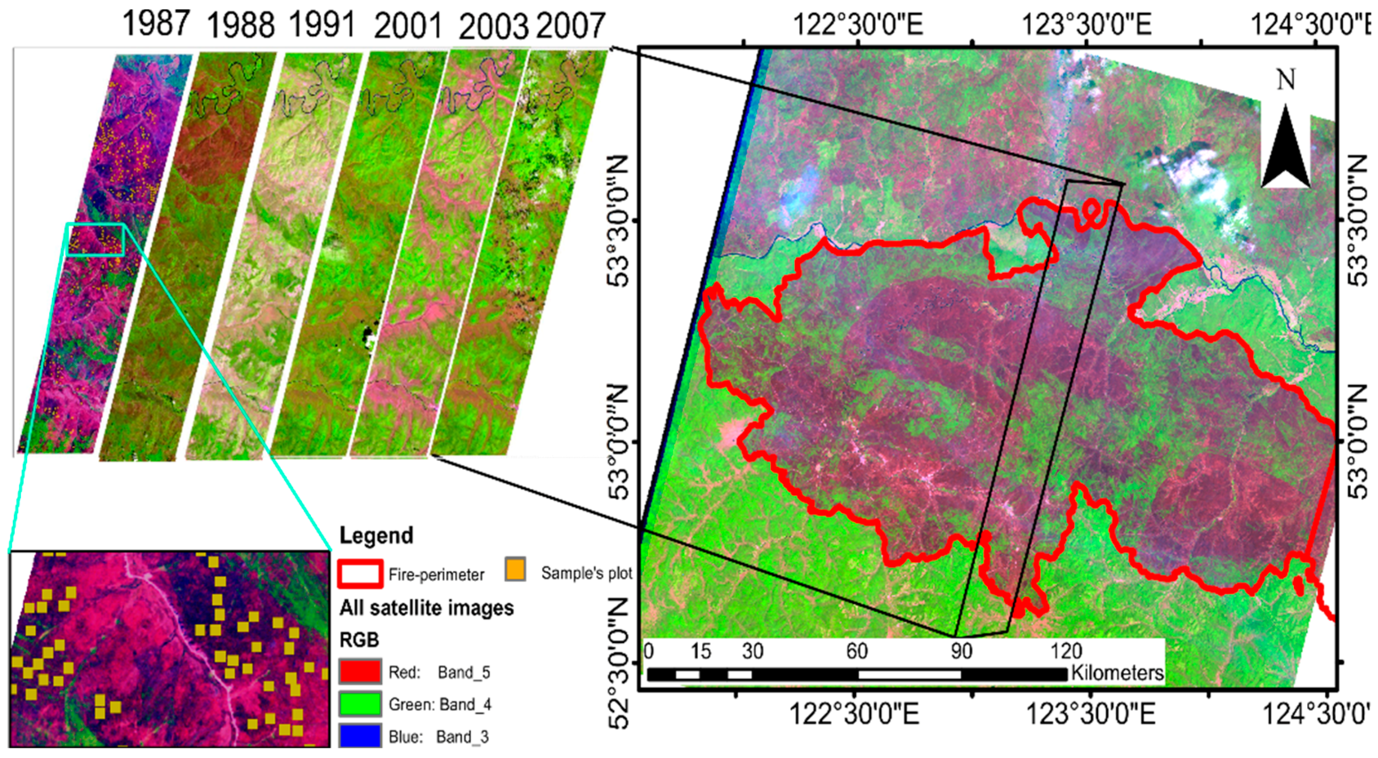
The multi-temporal data were obtained from a series of Landsat Thematic Mapper (TM) and Enhanced Thematic Mapper Plus (ETM+) (path 122 row 23) covering the period from 1987 to 2007: 15 June 1987 (TM), 17 June 1988 (TM), 10 June 1991 (TM), 21 June 2001 (TM), 11 June 2003 (TM), and 14 June 2007 (ETM+). Given data availability and quality, one system-corrected image per year was acquired to represent the phenological recovery stage. The resulting data set included 4 Landsat-5 TM and 2 Landsat-7 ETM+ pieces of data. The images were processed using the Level 1 Product Generation System (LPGS), version 12.8.3. To ensure the images were suitable for monitoring at different times, absolute atmospheric correction was completed for all multispectral data by using the Fast Line-of-sight Atmospheric Analysis of Hypercubes (FLAASH) module based on the Moderate Resolution Atmospheric Transmission Algorithm (MODTRAN).

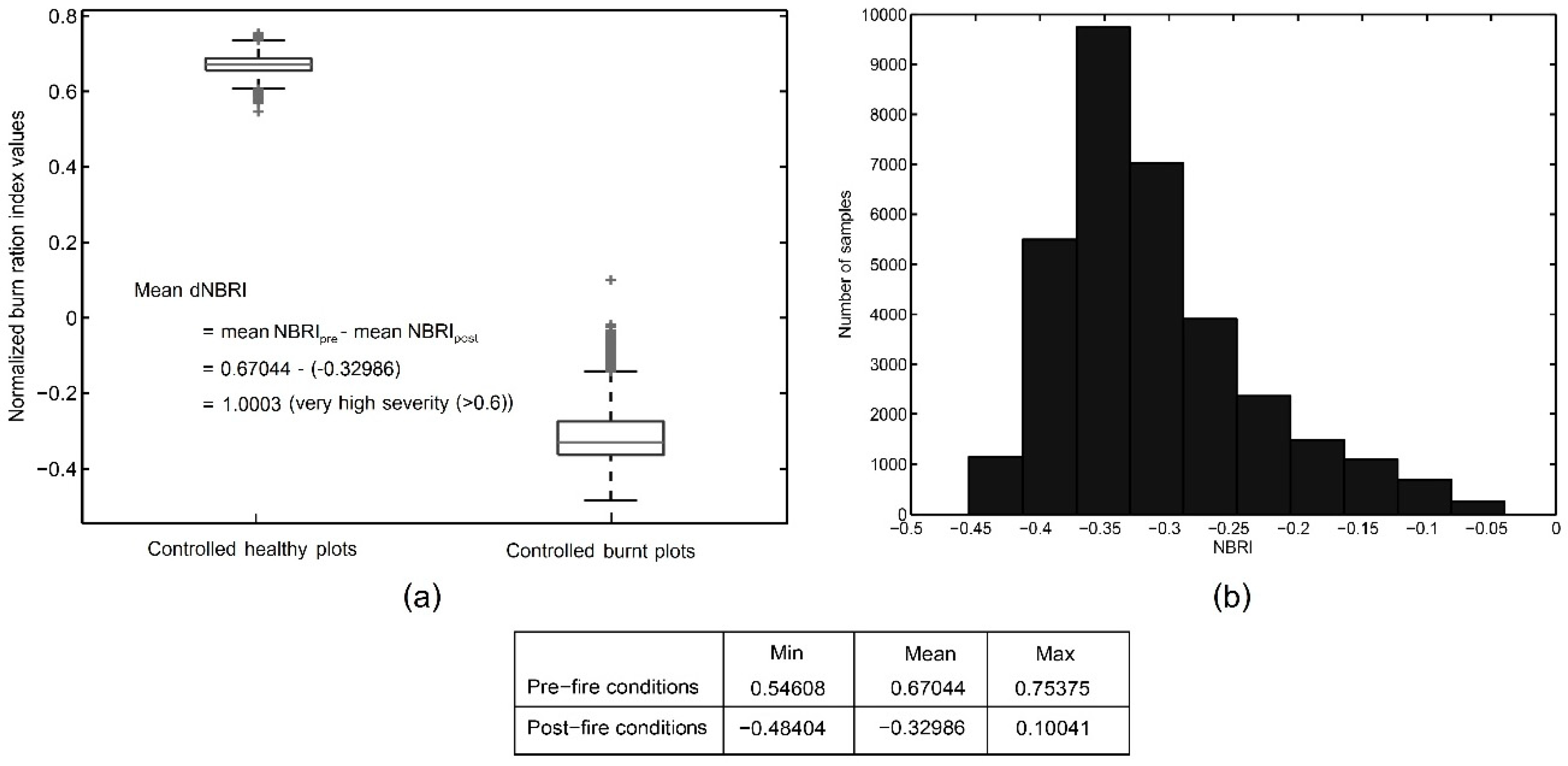
In addition to the satellite image data, a number of auxiliary vector datasets were obtained from our previous work, including ground survey data, human-interpreted fire perimeters for 1987 (Figure 1), and a thresholding-based fire-severity map. Unburnt samples were selected based on two criteria: (1) they should be close to the burnt sample and (2) must be determined as growth forest or undisturbed forest for a long time period, whereas burnt samples were acquired from within the high-severity area. The average and range of fire severity based on $\mathrm{dNBRI}$ (different normalized burn ratio index, $\mathrm{dNBRI} ={ \mathrm{NBRI} }_{\mathrm{prefire}}–{\mathrm{NBRI}}_{\mathrm{postfire}}$) were 1.0003 and 0.6533 to 1.0301, respectively. The NBRI’s distribution of the burnt samples at the fire year was shown in Figure 2.

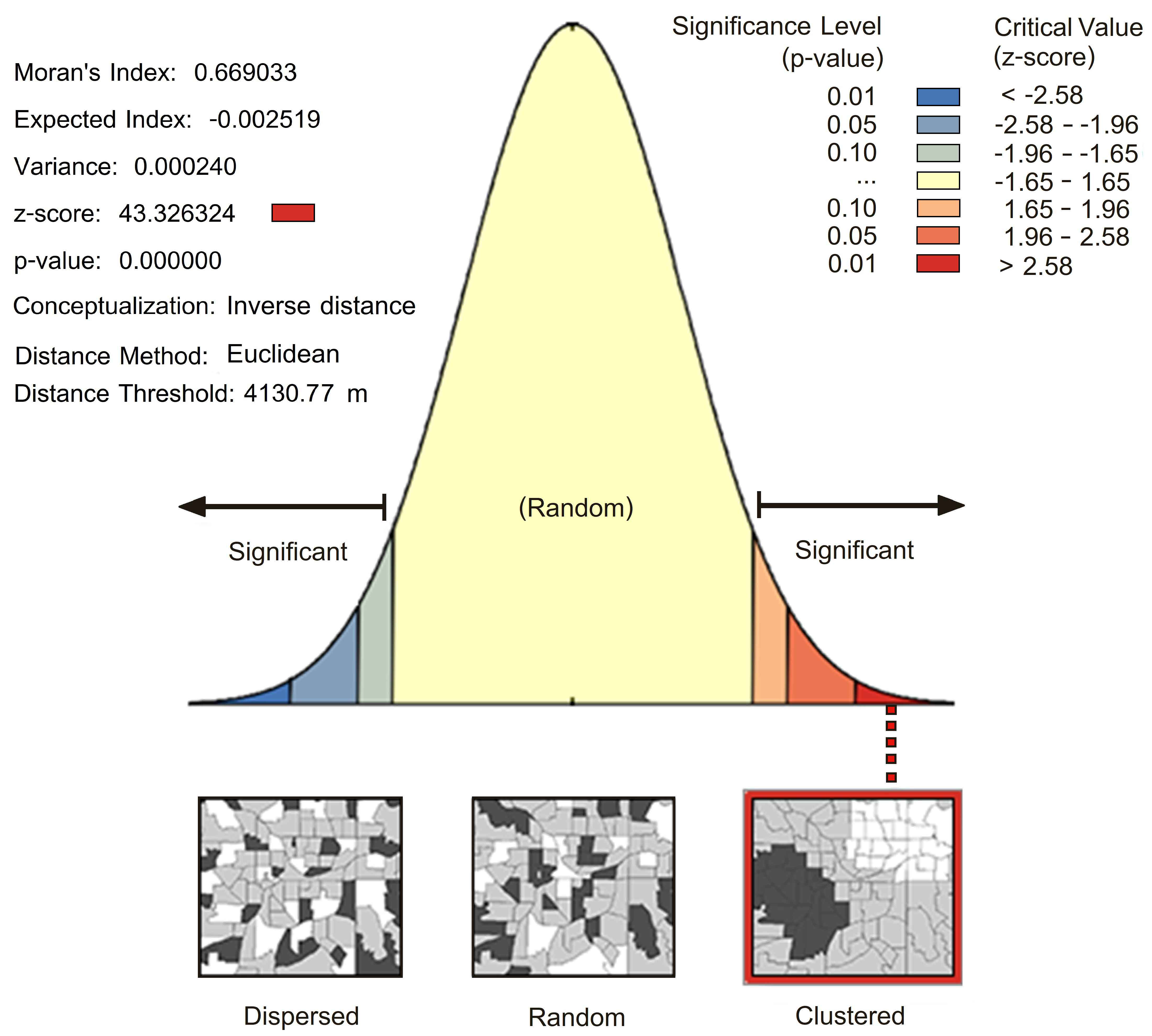
As mentioned above, we collected the training data in the areas where a high severity was known to exist. First, we located the center of training plots in the high severity areas. Figure 3 shows the spatial autocorrelation report of the training center points using Moran’s I technique [11]. Second, we created a square buffer (10 × 10 pixels) for each center points. Then, we used all of the pixels in the evaluation of RF-VIMP rank. This method produces highly clustered training sample points with significantly high spatial autocorrelation. The classification of the areas near the spatially autocorrelated training data will result in high classification accuracy because the areas outside these locations are not being tested [12].

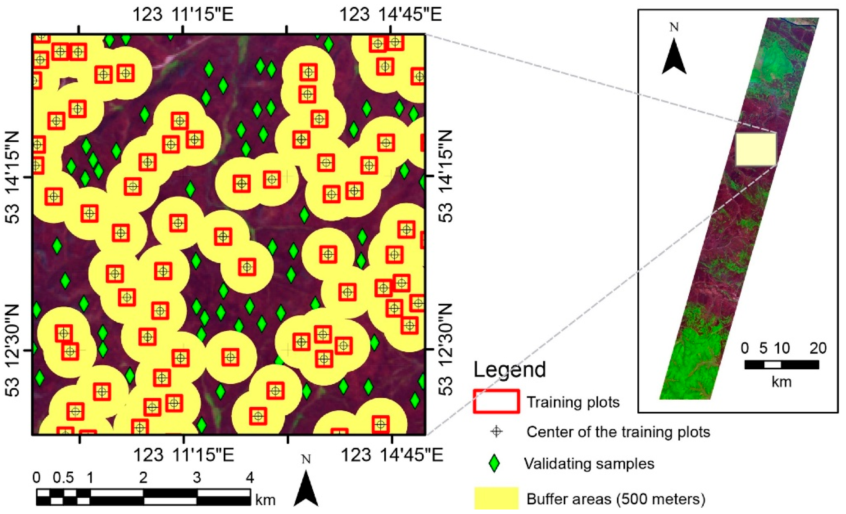
According to the suggestion in [12], to indicate that the positive spatial autocorrelation occurred in this study does not affect the final results of our framework, we assessed the classification accuracy of each spectral index regarding the recovering years using a new set of validating points. The validation points must follow these rules: (1) far from the center of the training data plots at least 500 m and (2) sparse over the study area (Figure 4). Note that the points were selected based on the fire year image, and the fire severity levels were varied. The geographic location of these points was used for the extraction of the validating samples of the other observation years. In this sense, the training data were randomly drawn, without replacement from the training plots, using a constant size of 6000 samples (3000 samples for each class). We reported the classification results using Kappa and overall accuracy (OA) by the averaging accuracy of 30 iterations.

2.2. Methods

2.2.1. Overview

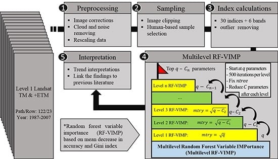
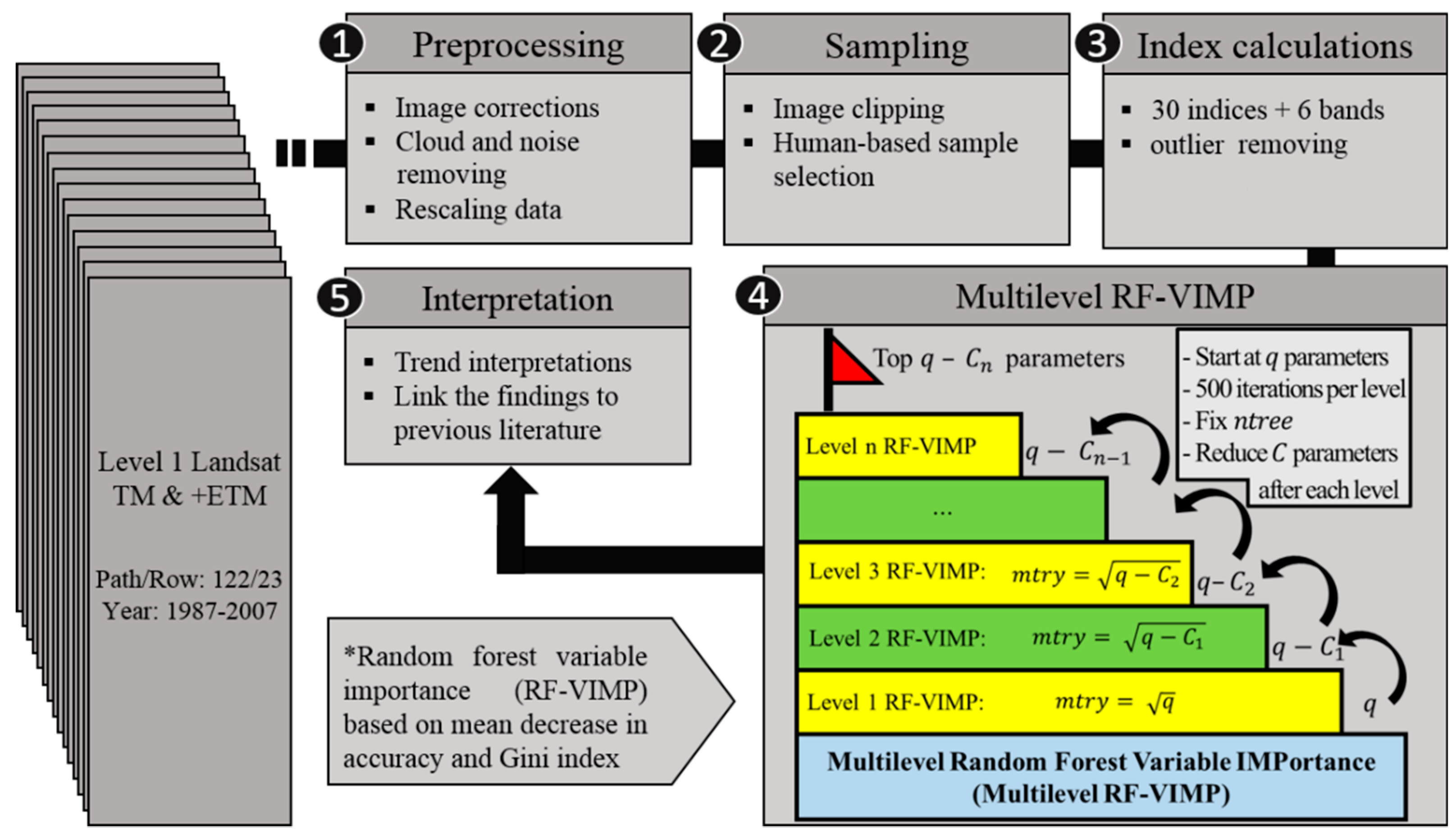
According to Figure 5, the system involves five steps. (1) The raw satellite images were corrected using the methods explained in Section 2.1, and then the corrected data were normalized into the range of [0, 1]. Although the random forest algorithm does not require transformed data, the rescaling can prevent numerical problems in the calculation and visualization of the result; (2) The samples were manually selected based on the high-severity area, as outlined in Section 2.1; (3) After evaluating spectral indices, we examined the box plot of each spectral index to detect and remove outliers (e.g., null data or very high and low value) caused by noise remaining in the corrected data; (4) The final samples were set as inputs to the multilevel RF-VIMP (Section 2.2.2); (5) The results from multilevel RF-VIMP were interpreted to examine the framework’s performance (Section 3 and Section 4).

2.2.2. Multilevel RF-VIMP System

The random forest algorithm estimates the importance of a variable by determining the amount by which the prediction error increases when out-of-bag ($oob$) data for that variable are permuted, whereas all other data items are left unchanged. The algorithm is a fully non-parametric technique and makes no assumptions about the residuals of the model. Specifically, including every tree grown in the forest, the $oob$ cases are recorded, and the number of votes cast for the correct class are counted. Then, a variable $\left(w\right)$ in the $oob$ case is randomly permuted, and these cases are moved down the tree. The number of votes for the correct class in the variable-$w$-permuted $oob$ data is subtracted from the number of votes for the correct class in the remaining $oob$ data. The importance score for w is computed by averaging the difference in the $oob$ error before and after the permutation for all trees. The score is normalized by the standard deviation of these differences. The variables, which produce large values for this score, are ranked as more important than features that produce small values [8].

Two types of importance measures exist: mean decrease in accuracy (MDA) and mean decrease in Gini index (MDG or Gini importance). The Gini importance measures the average gain of purity by splits of a given variable $w$. If the variable is useful, it tends to split mixed labeled nodes into pure single-class nodes. Permuting a useful variable tends to result in a relatively large decrease in mean Gini index. The MDA is the mean decrease of accuracy over all $oob$ cross-validated predictions when $w$ is permuted after training. Although both MDA and Gini importance were calculated in each iteration, the MDA was used as the main proxy in our decision process because it is more straightforward, easier to understand, more reliable [13], and more robust when it is averaged over all predictions [14]. We used an implementation of Random Forest’s R package in MATLAB [15] for calculating the MDA and Gini importance of each spectral index against forest recovery.

In this study, we implemented level 3 RF-VIMP (Figure 5, box 4) for 36 parameters (predictor variables) of 39,380 burnt and unburnt (response variables) samples from 1987, 1988, 1991, 2001, 2003, and 2007. In the first round of each year, the 36 parameters were evaluated for their delineation power in separating the burnt forest from the healthy forest using 500 RF-VIMP iterations. The same process was then applied to the second and third rounds, with the previous-round ranking of the top 30 and top 20 parameters, respectively. Then, only the top 10 parameters remaining from the last round were reported and discussed. The $mtry$ (square root of the predictor‘s number) were 6, 5, and 4 for the first, second, and third rounds, respectively. The interpretation of the random forest variable importance scores is only possible when the number of trees chosen is sufficiently large so that the results produced with different random seeds do not systematically vary. Thus, we set $ntree$ at 1000 for all iterations.

2.2.3. Spectral Index Acquisitions

The spectral index is a combination of single bands of remote sensing images and a simple, effective, and reliable form of ground feature characterization. In this study, 30 spectral indices and 6 band values (blue, green, red, near infrared, Short-wave infrared 1, and Short-wave infrared 2) were evaluated and examined to determine the relationship with forest recovery. The spectral indices are described in

Table 1. The spectral indices and equations used in this study.

Abbr.	Description	Equations
ARVI	Atmospherically resistant vegetation index	$\frac{NIR–R\times B}{NIR+R\times B}$
CTVI	Corrected transformed vegetation index	$\frac{NDVI + 0.5}{\left|NDVI + 0.5\right|}\times \sqrt{\left|NDVI + 0.5\right|}$
DVI	Difference vegetation index	$NIR–R$
EVI	Enhanced vegetation index [16]	$g\left[\frac{NIR–R}{NIR+C1\times R–C2\times B+L}\right], g= 2.5;C1=6;C2=7.5;L=1$
EVI2	Two-band enhanced vegetation index [17]	$g\left[\frac{NIR–R}{NIR+C1\times R+L}\right], g= 2.5; C1= 6; L= 1$
GARI	Green atmospherically resilient index [18]	$\frac{NIR–\left(G–\left(B–R\right)\right)}{NIR+\left(G–\left(B–R\right)\right)}$
GDVI	Green difference vegetation index	$NIR–G$
GEMI	Global environmental monitoring index	$\left(\frac{2\left(NI{R}^2-R^2\right)+1.5NIR+0.5R}{NIR+R+0.5}\right)\times \left(1-\left[\frac{2\left(NI{R}^2-R^2\right)+1.5NIR+0.5R}{NIR+R+0.5}\times 0.25\right]\right)-\left(\frac{R-0.125}{1-R}\right)$
GNDVI	Green normalized difference vegetation index	$\frac{NIR – G}{NIR + G}$
GRVI	Green ratio vegetation index [19]	$\frac{NIR}{G}$
GSAVI	Green soil-adjusted vegetation index [19]	$\left(\frac{NIR–G}{NIR+G+L}\right)\times \left(1+L\right),L= 0.5$
MNDWI	Modified normalized difference water index	$\frac{G–SWIR1}{G+SWIR1}$
MSAVI	Modified soil-adjusted vegetation index	$\frac{\left[\left(2NIR+1\right)–\sqrt{{\left(2 x NIR + 1\right)}^2–\left(8\left(NIR–R\right)\right)}\right]}{2}$
NBRI	Normalized burn ratio index [3]	$\frac{NIR – SWIR2}{NIR + SWIR2}$
NDVI	Normalized difference vegetation index	$\frac{NIR – R}{NIR + R}$
NDWI	Normalized difference water index [20]	$\frac{G – NIR}{G + NIR}$
NDWI2	Normalized difference water index 2 [7]	$\frac{NIR – SWIR1}{NIR + SWIR1}$
NG	Normalized green	$\frac{G}{NIR + R + G}$
NNIR	Normalized near-infrared	$\frac{NIR}{NIR + R + G}$
NR	Normalized red	$\frac{R}{NIR + R + G}$
NRVI	Normalized ratio vegetation index	$\frac{\frac{R}{NIR}– 1}{\frac{R}{NIR}+ 1}$.
OSAVI	Optimized soil-adjusted vegetation index [21]	$\frac{\left(NIR – R\right)\left(1 + L\right)}{NIR + R + L}, L = 0.16$
RVI	Ratio vegetation index (simple ratio)	$\frac{NIR}{R}$
SAVI	Soil-adjusted vegetation index	$\frac{\left(NIR-R\right)\left(1+L\right)}{NIR + R + L},L = 0.5$
TCB	Tasseled cap transformation brightness [22]	$\left(B\times 0.3561\right)+\left(G\times 0.3972\right)+ \left(R\times 0.3904\right)+\left(NIR\times 0.6966\right)+ \left(SWIR1\times 0.2286\right)+\left(SWIR2\times 0.1596\right)$
TCG	Tasseled cap transformation greenness [22]	$\left(B\times –0.3344\right)+\left(G\times –0.3544\right)+\left(R\times –0.4556\right)+\left(NIR\times 0.6966\right)+\left(SWIR1\times –0.0242\right)+\left(SWIR2\times –0.2630\right)$
TCW	Tasseled cap transformation wetness [22]	$\left(B\times 0.2626\right)+\left(G\times 0.2141\right)+ \left(R\times 0.0926\right)+\left(NIR\times 0.0656\right)+\left(SWIR1\times –0.7629\right)+\left(SWIR2\times –0.5388\right)$
TTVI	Thiam’s transformed vegetation index [23]	$\sqrt{\frac{\left|NIR – R\right|}{NIR + R} + 0.5}$
VARI	Visible atmospherically resistant index [24]	$\frac{G – R}{G + R – B}$
VIgreen	Vegetation index (green) [24]	$\frac{G – R}{G + R}$

Notations: B = Blue band, G = Green band, R = Red band, NIR = Near-infrared band, SWIR1 = Short-wave infrared band 1, SWIR2 = Short-wave infrared band 2.

below. Note that two-date-based indices (e.g., dNBRI and dNDVI) were determined to not be suitable for the study because the framework was designed for the year-by-year sequence of the forest succession stage. In particular, the interpretation of two-date-based indices is somewhat different to one-date-based indices. One-date-based indices can be directly linked to a particular forest succession stage, whereas the two-date-based indices generally refer to the change of the forest from a persistent stage.

3. Results

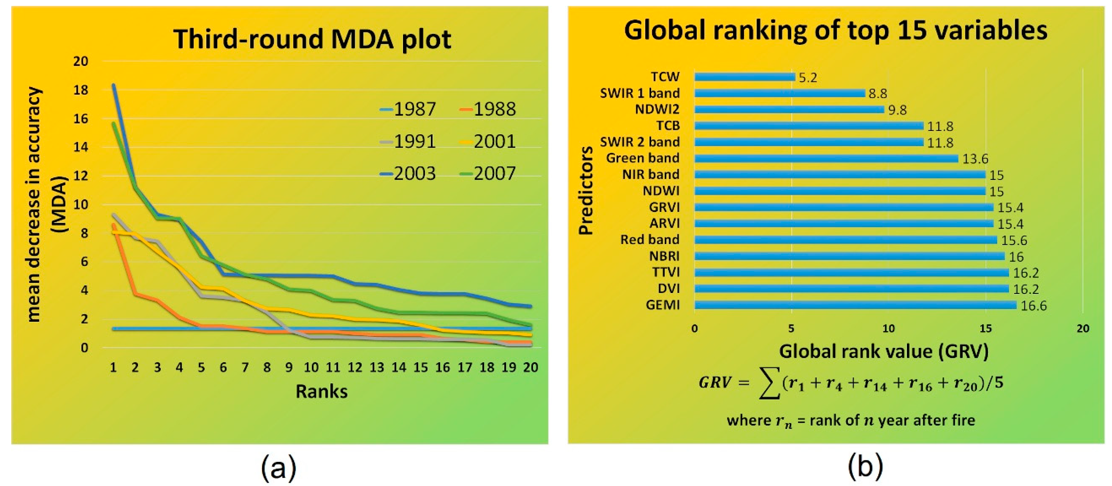
The average cumulative ranks were obtained from 500 iterations in third-round RF-VIMP, and the top 10 predictive parameters are presented in

Table 2. The variable ranks obtained from third-round RF-VIMP for all observation years.

Rank	Fire Year		1 Year after		4 Years after		14 Years after		16 Years after		20 Years after
	MDA	MDG	MDA	MDG	MDA	MDG	MDA	MDG	MDA	MDG	MDA	MDG
1	SWIR2	SWIR2	NBRI	NBRI	TCW	SWIR 2	SWIR 1	SWIR 1	Red	SWIR 1	TCB	TCB
2	EVI2	EVI2	NDWI2	SWIR2	NDWI2	TCW	TCB	TCW	Green	Red	NIR	NIR
3	NDWI	NDWI	SWIR2	NDWI2	SWIR 2	NDWI2	TCW	TCB	TCB	TCW	DVI	SWIR 1
4	SAVI	GRVI	NNIR	NNIR	NBRI	NBRI	NIR	SWIR 2	SWIR 1	Green	GEMI	GEMI
5	GRVI	SAVI	NRVI	EVI2	Blue	SWIR 1	GEMI	NIR	TCW	SWIR 2	EVI	EVI
6	NIR	NIR	TCW	NRVI	SWIR 1	Red	DVI	MNDWI	NIR	Blue	GDVI	DVI
7	CTVI	CTVI	ARVI	TTVI	ARVI	ARVI	SWIR 2	GDVI	NRVI	TCB	SWIR 1	GDVI
8	GEMI	GEMI	TTVI	NDVI	Red	Green	NDWI2	GEMI	TTVI	ARVI	CTVI	Green
9	ARVI	ARVI	NDVI	RVI	Green	Blue	GDVI	NDWI2	NDVI	Vig	SAVI	Blue
10	NBRI	NBRI	RVI	NR	GNDVI	TTVI	CTVI	DVI	RVI	NIR	Green	CTVI

and Figure 6. The results based on both MDA and MDG (Table 2) consistently suggest that SWIR1 (1.55–1.75 μm) and SWIR2 (2.08–2.35 μm) were the key predictive indicator for forest recovery in the study area, as they usually ranked in the high rank for all observation years. Almost all parameters achieved identical MDA in the year of the fire (1987) (Figure 6a,

Table 3. The classification accuracy by the RF classifier ($ntree=1000;mtry=1$) of each predictor against the validating samples of all observed years.

Indices	1 Year after		4 Years after		14 Years after		16 Years after		20 Years after		GRV	Ranks *
	R *	K *	R	K	R	K	R	K	R	K
SWIR2	2	0.96	1	0.99	2	0.86	2	0.68	6	0.50	2.6	1
SWIR1	33	0.66	4	0.97	1	0.96	1	0.81	1	0.73	8	2
TCW	18	0.88	3	0.99	4	0.83	7	0.43	10	0.40	8.4	3
Red	16	0.91	2	0.99	6	0.70	3	0.62	19	0.28	9.2	4
NDWI2	19	0.87	10	0.92	5	0.75	5	0.51	7	0.43	9.2	5
TCB	36	0.29	6	0.96	3	0.83	4	0.53	2	0.66	10.2	6
NBRI	3	0.94	7	0.96	10	0.46	10	0.31	21	0.25	10.2	7
NIR	32	0.71	17	0.90	7	0.61	6	0.48	4	0.51	13.2	8
NDWI	9	0.93	11	0.91	17	0.23	13	0.29	28	0.19	15.6	9
ARVI	1	0.96	8	0.93	23	0.20	11	0.30	36	0.08	15.8	10
NRVI	8	0.93	12	0.91	18	0.23	15	0.29	26	0.20	15.8	11
RVI	7	0.93	13	0.91	16	0.24	12	0.30	31	0.18	15.8	12
MNDWI	34	0.49	27	0.65	8	0.57	8	0.37	3	0.57	16	13
Green	6	0.93	14	0.91	19	0.23	14	0.29	32	0.18	17	14
TTVI	14	0.92	5	0.97	11	0.35	22	0.23	34	0.16	17.2	15

* R = Rank; K = Kappa accuracy; Ranks are based on based on GRV.

), because burnt and healthy forest were easy to separate. However, there are six indices (green band, MNDWI, SWIR1, TCB, TCW, VARI, and VIgreen) that received a 0 value that are not shown in the results for either MDA or MDG, representing a low discriminative ability when competing to the other predictors. Based on the RF-VIMP, one year after fire, the NBRI was the most predictive index. Moreover, NIR and SWIR2 alternated in terms of being ranked first from 4 to 16 years after the fire.

The tasseled-cap indices gradually increased in rank until reaching the top five ranking in the final observation year, 20 years after the fire, especially for the TCB and TCW. We introduced the calculation of the global rank value (GRV) as shown in Figure 6b to assess the predictive value of all parameters against all observation years excluding the fire year. Consequently, the GRV scores confirmed that TCW, TCB, and SWIR (both 1 and 2)-based indices were the predictive indicator, followed by the red, green, and NIR band-based indices, etc. (Figure 6b).

4. Discussion

4.1. Biases in the Importance Value Calculated from the Random Forest Algorithm

The research conducted by Strobl et al. [13] found that, for the Breiman’s random forest method, the variable importance measures were affected by the number of categories and scale of measurement of the predictor variables, which are no direct indicators of the actual importance of the variable, particularly in the genomics and computational biology where both of continuous (i.e., folding energy) and categorical (i.e., amino acid sequence) predictors appear in the data set. In addition, the original RF-VIMP should not be used when the potential predictor variables vary in their scale of measurement or their number of categories. The work also indicates that the Gini importance (referred as MDG in this study) is more strongly biased than permutation importance (referred as MDA in this study).

To achieve unbiased VIMP values, the conditional variable importance (cforest), which can assess true impact of each predictor variable, was proposed by Strobl et al. [14]. The cforest is available in R add-on “party” package [25,26]. However, the results in [13] show that the variable importance measured from the scaled permutation method of the original RF-VIMP and one from cforest method shared the identical most-informative variable. This indicates that we can still trust the high-rank variable from the original RF-VIMP with the scaled permutation method.

The characteristics of the predictors (spectral profiles and indices) used in our study are different. A notice stated in [13] indicates that the original random forest variable importance measure is not affected if the predictors are only continuous predictor variables or only variables with the same number of categories. This is the case for the predictors in our study, since they are actually continuous variables. Moreover, we used the permutation importance as the main parameter in variable selection. Please note that the proposed framework in this study is not limited to the Breiman’s RF-VIMP, it is also suitable for other random forest variable importance measures (i.e., cforest).

4.2. The Random Forest Algorithm vs. Multicollinearity and Spatial Autocorrelation

Multicollinearity refers to the existence of high inter-correlations (near-linear dependencies) among the independent variables in multiple linear regression analysis. When severe multicollinearity exists, the following problems may occur [27,28]: (1) small changes in the data can produce significant changes in the correlation coefficients (more sensitivity); (2) the regression coefficients may have high standard errors, which affect the significance level of the corresponding independent variable, and may have an unreliable magnitude and sign [29]. Spatial autocorrelation implies a lack of spatial independence; that is, the samples are not statistically independent on one another. When events are clustered together, we refer to this arrangement as positive spatial autocorrelation. On the other hand, an arrangement where events are extremely dispersed is referred to as negative spatial autocorrelation. A potential problem with satellite data is that the spectral profile in neighboring sampling units are likely to be similar because the satellite pixels are generally smaller than the land cover (i.e., forest fire areas). This can result in positive spatial autocorrelation which causes problems for statistical methods that make assumptions about the independence of residuals (a residual is a difference between an observed and a predicted value) [30,31,32,33]. For example, most classical statistical analyses (i.e., ordinary least squares regression) are based on the assumption that the values of observations in each sample are independent of one another. The correlation coefficients will be biased, and their precision inflated [29,34]. Therefore, the effects of multicollinearity and spatial autocorrelation are significantly severe in the classical statistic methods (especially for regression analysis), and the detection of those problems should be applied.

Conversely, the above phenomena may not affect the RF-VIMP framework for the following reasons: (1) the RF algorithm is a fully non-parametric technique, it makes no assumptions about the data distribution and the residuals of the model [35,36]; (2) The technique is well suited to the analysis of highly collinear data sets with a very large number of predictor variables and does not assume a linear relationship between predictor variables [8,15,37,38] and correlated predictor variables [37,39]. Based on these characteristics, the RF has been widely used in many prior studies to assess the effect of predictor variables on land cover change [40,41]. However, recent research by Millard and Richardson [12] suggests reporting the spatial autocorrelation level in the RF classification. The RF classification accuracy’s report would be unclear if the level of spatial autocorrelation in the training data were not observed. This is the reason why we confirmed the RF-VIMP rank by measuring the RF classification accuracy of the data from the separate validating data (see also Section 2.1). The investigation indicates that the classification’s results are consistent with the multilevel RF-VIMP results (Table 3). Note that the predictive rank from the classification using the separate validating set was different from the RF-VIMP rank by the following reasons: (1) the separate validating set has a wide range of fire severity while the fire severity for the data set of RF-VIMP is limited to very high severity; (2) The parameter $mtry$ in the classification using a single predictor is less than (i.e., $mtry$=1) the RF-VIMP framework (i.e., $mtry=\left\{6,5,4\right\}$).

4.3. Variable Importances and Forest Succession

As mentioned above, distinguishing between burnt and healthy forest using satellite data is rather easy because their histograms are far apart [3]. The results from the system were not only consistent with previous findings, but also proved that most indices observed in this study can be used for classification since they had an equal MDA value in the year of the fire. However, the green band, MNDWI, SWIR1, TCB, TCW, VARI, and VIgreen methods might be inappropriate for classification in the fire year or have less discriminative ability than the others, as they acquired an MDA of zero. Most of these methods are not based on the near-infrared band, which is the most essential parameter for early post-fire monitoring in the first five years after fire [42]. The NIR band is normally affected by the leaf structure and the red band is affected by chlorophyll, for which the leaf conditions significantly fluctuate during the early succession process. Consequently, most NIR and red reflectance-based indices acquired a high ranking in the early post-fire years (Table 2), which conforms to the results published by Lopez-Garcia and Casselle [43]. The blue band was usually ranked lower because it is commonly affected by scattered light. For the green band and its related indices, a moderate relationship with forest succession existed as it remained at the medium rank in almost all observation years. However, the previous findings revealed that incorporating the green band in the ratio-based indices improved the prediction of leaf area index (LAI), which is a popular ground-based monitoring proxy in forest health analysis [44].

Several studies concluded that incorporating short-wave infrared bands [45] (e.g., NBRI and NDWI2) to analyze burn severity provides the highest accuracies [46,47]. Post-fire recovery in boreal larch ecosystems is more strongly correlated with SWIR1-based indices than NIR- and red-based indices [6]. One of the reasons for this is that SWIR1-based indices are more sensitive to vegetation structure and are capable of highlighting large dynamic changes [48,49]. Table 2 and Table 3 show that SWIR1 was significant for long-term monitoring after 14 years of recovery.

In conclusion, the results of this study suggest that shortwave infrared bands and their compound indices are the key predictive variables for burnt forest recovery in the study area. They had a distinctive GRV value, whereas other compound indices had similar GRV values. Notably, the importance of the tasseled-cap indices, especially for the TCB and TCW, gradually increased with the forest succession. In addition to the high discriminatory power of SWIR bands, we suggest that a new SWIR-based index should be developed as a compound index to provide additional insight into environmental conditions compared with the pure SWIR bands alone. The results in Table 3 indicate that SWIR bands may be suitable for long-term forest monitoring because they continue to provide high classification accuracy (in all observation years) to validate samples with a wide range of fire severity. Additionally, more parameters, in particularly those related to the environment, should be investigated to confirm our findings.

In this paper, we stopped the process at the third level for two reasons: (1) the variables did not change their rank, noting that in the top rank, we focused on the top five variables; and (2) we reduced the number of variables by 10 at each level. Consequently, the process should stop at third-level, since we had only 36 variables. The proposed multilevel RF-VIMP method can be performed many times, as it allows the user to determine the level at which it should be stopped. The application of a multilevel RF-VIMP system may not be limited to representing the spectral indices and burnt forest recovery relationship, but may also be used as a tool for designing a new index more appropriate for specific tasks in the future.

5. Conclusions

The multilevel RF-VIMP system is a method for finding relationships in burnt forest recovery using remote sensing data based on the random forest variable importance algorithm (RF-VIMP). RF-VIMP uses burnt and healthy forest samples from a single date in the algorithm, finding the mean decrease in accuracy when a predictor is omitted, whereas the other predictors are fixed. The process is then repeated for the rest of the predictors. These results represent a loss in accuracy of the predictor compared with other predictors in the system in terms of discriminative power. For the first time, we proposed applying the RF-VIMP concept to multidate-series satellite data for a burnt forest area. The experiment showed that by following the multilevel RF-VIMP scheme, the importance value not only refers to discriminative ability, but can also be used as a proxy to address the relationship between predictors (spectral indices) and forest succession. The results based on MDA suggest that the TCB, TCW, and SWIR bands are the key variables for observing forest succession in the study area, out of 36 remote sensing parameters. In addition, the proposed method clearly shows the dynamics of spectral indices as the forest recovers over time. This method is easy to apply and can handle a large number of predictors at a time. We suggest applying the method to monitor and investigate more specific parameters such as ground-survey-based indices of environmental conditions.

References

- Qu, J.; Hao, X.; Liu, Y.; Riebau, A.; Yi, H.; Qin, X. Remote Sensing Applications of Wildland Fire and Air Quality in China. Dev. Envi. Sci. 2016, 8, 277–288. [Google Scholar]
- Tian, X.; McRae, D.J.; Jin, J.; Shu, L.; Zhao, F.; Wang, M. Changes of Forest Fire Danger and the Evaluation of the FWI System Application in the Daxing’ anling Region. Sci. Silv. Sin. 2010, 46, 127–132. [Google Scholar]
- Chen, W.; Sakai, T.; Moriya, K.; Koyama, L.; Cao, C. Extraction of burned forest area in the Greater Hinggan Mountain of China based on Landsat TM data. In Proceedings of the 2013 IEEE International Geoscience and Remote Sensing Symposium (IGRASS), Melbourne, Australia, 21–26 July 2013. [Google Scholar]
- Santis, D.A.; Chuvieco, E. Burn severity estimation from remotely sensed data: Performance of simulation versus empirical models. Remote Sens. Environ. 2007, 108, 422–435. [Google Scholar] [CrossRef]
- Yi, K.; Tani, H.; Zhang, J.; Guo, M.; Wang, X.; Zhong, G. Long-term satellite detection of post-fire vegetation trends in boreal forests of China. Remote Sens. 2013, 5, 6938–6957. [Google Scholar] [CrossRef]
- Liu, Z. Effects of climate and fire on short-term vegetation recovery in the boreal larch forests of Northeastern China. Sci. Rep. 2016, 6, 37572. [Google Scholar] [CrossRef] [PubMed]
- Gao, B.C. NDWI A Normalized Difference Water Index for remote sensing of vegetation liquid water from space. Remote Sens. Environ. 1996, 58, 257–266. [Google Scholar] [CrossRef]
- Breiman, L. Random Forests. Mach. Learn. 2001, 45, 5–32. [Google Scholar] [CrossRef]
- Schroeder, T.; Schleeweis, K.; Moisen, G.; Toney, C.; Cohen, W.; Freeman, E.; Yang, Z.; Huang, C. Testing a Landsat-based approach for mapping disturbance causality in U.S. forests. Remote Sens. Environ. 2017, 195, 230–243. [Google Scholar] [CrossRef]
- Han, J.; Shen, Z.; Ying, L.; Li, G.; Chen, A. Early post-fire regeneration of a fire-prone subtropical mixed Yunnan pine forest in Southwest China. For. Ecol. Manag. 2015, 356, 31–40. [Google Scholar] [CrossRef]
- Moran, P.A.P. Notes on Continuous Stochastic Phenomena. Biometrika 1950, 37, 17–23. [Google Scholar] [CrossRef] [PubMed]
- Millard, K.; Richardson, M. On the importance of training data sample selection in random forest image classification: A case study in peatland ecosystem mapping. Remote Sens. 2015, 7, 8489–8515. [Google Scholar] [CrossRef]
- Strobl, C.; Boulesteix, A.L.; Zeileis, A.; Hothorn, T. Bias in random forest variable importance measures: Illustrations, sources and a solution. Bioinformatics 2007, 8. [Google Scholar] [CrossRef] [Green Version]
- Strobl, C.; Boulesteix, A.L.; Kneib, T.; Augustin, T.; Zeileis, A. Conditional variable importance for random forests. Bioinformatics 2008, 9, 307. [Google Scholar] [CrossRef] [PubMed] [Green Version]
- Liaw, A.; Wiener, M. Classification and regression by Random Forest. R News 2002, 2, 18–22. [Google Scholar]
- Huete, A.; Didan, K.; Miura, T.; Rodriguez, E.; Gao, X.; Ferreira, L. Overview of the radiometric and biophysical performance of the MODIS vegetation indices. Remote Sens. Environ. 2002, 83, 195–213. [Google Scholar] [CrossRef]
- Jiang, Z.; Huete, A.; Didan, K.; Miura, T. Development of a two-band enhanced vegetation index without a blue band. Remote Sens. Environ. 2008, 112, 3833–3845. [Google Scholar] [CrossRef]
- Gitelson, A.; Kaufman, Y.; Merzlyak, M. Use of a green channel in remote sensing of global vegetation from EOS-MODIS. Remote Sens. Environ. 1996, 58, 289–298. [Google Scholar] [CrossRef]
- Sripada, R.; Heiniger, R.; White, J.; Meijier, A. Aerial color infrared photography for determining early-season in-season nitrogen requirements in corn. Agron. J. 2006, 98, 968–977. [Google Scholar] [CrossRef]
- Mcfeeters, S. The use of normalized difference water index (NDWI) in the delineation of open water feature. Int. J. Remote Sens. 1996, 17, 1425–1432. [Google Scholar] [CrossRef]
- Rondeaux, G.; Steven, M.; Baret, F. Optimization of soil-adjusted vegetation indices. Remote Sens. Environ. 1996, 55, 95–107. [Google Scholar] [CrossRef]
- Huang, C.; Wylie, B.; Yang, L.; Homer, C.; Zylstra, G. Derivation of a tasselled cap transformation based on Landsat 7 at-satellite reflectance. Int. J. Remote Sens. 2002, 23, 1741–1748. [Google Scholar] [CrossRef]
- Thiam, A. Geographic Information Systems and Remote Sensing Methods for Assessing and Monitoring Land Degradation in the Sahel: The Case of Southern Mauritania. Ph.D. Thesis, Clark University, Worcaster, MA, USA, 1997. [Google Scholar]
- Gitelson, A.; Kaufman, Y.; Stark, R.; Rundquist, D. Novel algorithms for remote estimation of vegetation fraction. Remote Sens. Environ. 2002, 80, 76–87. [Google Scholar] [CrossRef]
- Strobl, C.; Hothorn, T.; Zeileis, A. Party on! A new, conditional variable-importance measure for random forests available in the party package. R J. 2009, 1, 14–17. [Google Scholar]
- Hothorn, T.; Hornik, K.; Zeileis, A. Party: A Laboratory for Recursive Part(y)itioning. 2006. Available online: http://CRAN.R-project.org (accessed on 19 April 2018).
- Kleinbaum, D.G.; Kupper, L.L.; Muller, K.E. Applied Regression Analysis and Other Multivariable Methods; PWS-Kent Publishing Company: Boston, MA, USA, 1988. [Google Scholar]
- Myers, R.H. Classical and Modern Regression with Applications; Duxbury Press: Duxbury, MA, USA, 1986. [Google Scholar]
- Kozak, A. Effects of multicollinearity and autocorrelation on the variable-exponent taper functions. Can. J. For. Res. 1997, 27, 619–629. [Google Scholar] [CrossRef]
- Sokal, R.R.; Oden, N.L. Spatial autocorrelation in biology 1. Methodology. Biol. J. Linn. Soc. 1978, 10, 199–228. [Google Scholar] [CrossRef]
- Sokal, R.R.; Thomson, J.D. Applications of spatial autocorrelation in ecology. In Developments in Numerical Ecology; NATO ASI Series; Legendre, P., Legendre, L., Eds.; Springer: Berlin, Germany, 1987; p. G14. [Google Scholar]
- Klinkenberg, B. Geob 479—GIScience in Research. Available online: http://ibis.geog.ubc.ca/courses/geob479/notes/spatial_analysis/spatial_autocorrelation.htm (accessed on 19 April 2018).
- Mascaro, J.; Asner, G.P.; Knapp, D.E.; Kennedy-Bowdoin, T.; Martin, R.E.; Anderson, C.; Higgins, M.; Chadwick, K.D. A tale of two “forests”: Random forest machine learning aids tropical forest carbon mapping. PLoS ONE 2014, 9. [Google Scholar] [CrossRef] [PubMed]
- Griffith, D. Spatial Autocorrelation: A Primer; Association of American, Geographers Resource Publication: Washington, DC, USA, 1987. [Google Scholar]
- James, G.; Witten, D.; Hastie, T.; Tibshirani, R. An Introduction to Statistical Learning with Application in R; Springer: New York, NY, USA, 2013. [Google Scholar]
- Rao, M.; George, L.A.; Shandas, V.; Rosenstiel, T.N. Assessing the Potential of Land Use Modification to Mitigate Ambient NO2 and Its Consequences for Respiratory Health. Int. J. Environ. Res. Public Health 2017, 14, 750. [Google Scholar] [CrossRef] [PubMed]
- Svetnik, V.; Liaw, A.; Tong, C.; Culberson, J.C.; Sheridan, R.P.; Feuston, B.P. Random forest: A classification and regression tool for compound classification and QSAR modeling. J. Chem. Inf. Comp. Sci. 2003, 43, 1947–1958. [Google Scholar] [CrossRef] [PubMed]
- Bax, V.; Francesconi, W. Environmental predictors of forest change: An analysis of natural predisposition to deforestation in the tropical Andes region, Peru. Appl. Geogr. 2018, 91, 99–110. [Google Scholar] [CrossRef]
- Evans, J.S.; Murphy, M.A.; Holden, Z.A.; Cushman, S.A. Modeling species distribution and change using Random Forests. In Predictive Species and Habitat Modeling in Landscape Ecology: Concepts and Applications; Drew, C.A., Wiersma, Y.F., Huettmann, F., Eds.; Springer: New York, NY, USA, 2011. [Google Scholar]
- Oliveira, S.; Oehler, F.; San-Miguel-Ayanz, J.; Camia, A.; Pereira, J.M. Modeling spatial patterns of fire occurrence in Mediterranean Europe using Multiple regression and random forest. For. Ecol. Manag. 2012, 275, 117–129. [Google Scholar] [CrossRef]
- Sánchez-Cuervo, A.M.; Aide, T.M. Consequences of the armed conflict, forced human displacement, and land abandonment on forest cover change in Colombia: A multi-scaled analysis. Ecosystems 2013, 16, 1052–1070. [Google Scholar] [CrossRef]
- Meng, R.; Wu, J.; Schwager, K.; Zhao, F.; Dennison, P.; Cook, B.; Brewster, K.; Green, T.; Serbin, S. Using high spatial resolution satellite imagery to map forest burn severity across spatial scales in a Pine Barrens ecosystem. Remote Sens. Environ. 2017, 191, 95–109. [Google Scholar] [CrossRef]
- García, M.J.L.; Caselles, V. Mapping burns and natural reforestation using thematic Mapper data. Geocarto Int. 1991, 6, 31–37. [Google Scholar] [CrossRef]
- Masemola, C. Remote Sensing of Leaf Area Index in Savannah Grass Using Inversion of Radiative Transfer Model on Landsat 8 Imagery: Case Study Mpumalanga, South Africa. Ph.D. Thesis, University of South Africa, Pretoria, South Africa, 2015. [Google Scholar]
- Nioti, F.; Xystrakis, F.; Koutsias, N.; Dimopoulos, P. A Remote Sensing and GIS Approach to Study the Long-Term Vegetation Recovery of a Fire-Affected Pine Forest in Southern Greece. Remote Sens. 2015, 7, 7712–7731. [Google Scholar] [CrossRef]
- Cocke, A.E.; Fulé, P.Z.; Crouse, J.E. Comparison of burn severity assessments using Differenced Normalized Burn Ratio and ground data. Int. J. Wildland Fire 2005, 14, 189–198. [Google Scholar] [CrossRef]
- Chen, X.; Zhu, Z.; Ohlen, D.; Huang, C.; Shi, H. Use of multiple spectral indices to estimate burn severity in the black hills of South Dakota. In Proceedings of the Pecora 17—The Future of Land Imaging Going Operational, Denver, CO, USA, 18–20 November 2008. [Google Scholar]
- Cuevas-gonzalez, M.; Gerard, F.; Balzter, H.; Riano, D. Analysing forest recovery after wildfire disturbance in boreal forest regions: A review. Remote Sens. 2014, 6, 470–520. [Google Scholar]
- Ollinger, S. Sources of variability in canopy reflectance and the convergent properties of plants. New Phytol. 2011, 189, 375–394. [Google Scholar] [CrossRef] [PubMed]
Figure 1.
The perimeter of the fire area obtained from Chen et al. [3] and the sample plots distribution on the high-severity area.
Figure 2.
(a) The box plots of the burnt and unburnt NBRI of the training samples and the calculation of the mean dNBRI; (b) The histogram of NBRI distribution in the training burnt samples.
Figure 3.
The spatial autocorrelation report from the Moran’s I technique of the ArcMap 10.2.2 software. The figure indicates that there is a high spatial autocorrelation in this study.
Figure 4.
The location of training plots, training centers, and validating samples. Note that the illustration is a part of the study area.
Figure 5.
The multilevel random forest variable importance (RF-VIMP) system for burnt forest recovery monitoring.
Figure 6.
(a) Comparison plot of mean decrease in accuracy using the third-round RF-VIMP of each observation year; (b) the global ranking of the top 15 variables.