Article

A Cloud-Based Multi-Temporal Ensemble Classifier to Map Smallholder Farming Systems

Faculty of Geo-Information Science and Earth Observation (ITC). University of Twente, 7514 AE Enschede, The Netherlands
*
Author to whom correspondence should be addressed.
Remote Sens. 2018, 10(5), 729; https://doi.org/10.3390/rs10050729
Submission received: 30 March 2018 / Revised: 2 May 2018 / Accepted: 7 May 2018 / Published: 9 May 2018
(This article belongs to the Collection Google Earth Engine Applications)

Abstract

:
Smallholder farmers cultivate more than 80% of the cropland area available in Africa. The intrinsic characteristics of such farms include complex crop-planting patterns, and small fields that are vaguely delineated. These characteristics pose challenges to mapping crops and fields from space. In this study, we evaluate the use of a cloud-based multi-temporal ensemble classifier to map smallholder farming systems in a case study for southern Mali. The ensemble combines a selection of spatial and spectral features derived from multi-spectral Worldview-2 images, field data, and five machine learning classifiers to produce a map of the most prevalent crops in our study area. Different ensemble sizes were evaluated using two combination rules, namely majority voting and weighted majority voting. Both strategies outperform any of the tested single classifiers. The ensemble based on the weighted majority voting strategy obtained the higher overall accuracy (75.9%). This means an accuracy improvement of 4.65% in comparison with the average overall accuracy of the best individual classifier tested in this study. The maximum ensemble accuracy is reached with 75 classifiers in the ensemble. This indicates that the addition of more classifiers does not help to continuously improve classification results. Our results demonstrate the potential of ensemble classifiers to map crops grown by West African smallholders. The use of ensembles demands high computational capability, but the increasing availability of cloud computing solutions allows their efficient implementation and even opens the door to the data processing needs of local organizations.

Graphical Abstract

1. Introduction

Smallholder farmers cultivate more than 80% of the cropland area available in Africa [1] where the agricultural sector provides about 60% of the total employment [2]. However, the inherent characteristics of smallholder farms such as their small size (frequently less than 1 ha and with vaguely delineated boundaries), their location in areas with extreme environmental variability in space and time, and the use of mixed cropping systems, have prevented a sustainable improvement on smallholder agriculture in terms of volume and quality [3]. Yet, an increase of African agricultural productivity is imperative because the continent will experience substantial population growth in the coming decades [4]. Realizing that croplands are scarce, the productivity increase should have the lowest reasonable environmental impact and should be as sustainable as possible [5]. A robust agricultural monitoring system is then a prerequisite to promote informed decisions not only at executive or policy levels but also at the level of daily field management. Such a system could, for example, help to reduce price fluctuations by deciding on import and export needs for each crop [6], to establish agricultural insurance mechanisms, or to estimate the demand for agricultural inputs [6,7]. Crop maps are a basic but essential layer of any agricultural monitoring system and are critical to achieve food security [8,9]. Most African countries, however, lack reliable crop maps. Remote sensing image classification is a convenient approach for producing these maps due to advantages in terms of cost, revisit time, and spatial coverage [10]. Indeed, remotely sensed image classification has been successfully applied to produce crop maps in homogeneous areas [11,12,13,14].
Smallholder farms, which shape the predominate crop production systems in Africa, present significant mapping challenges compared to homogeneous agricultural areas (i.e., with intensive or commercial farms) [8]. Difficulties are not only in requiring very high spatial resolution data, but also in the spectral identification of farm fields and crops because smallholder fields are irregularly shaped and their seasonal variation in surface reflectance is strongly influenced by irregular and variable farm practices in environmentally diverse areas. Because of these peculiarities, the production of reliable crop maps from remotely sensed images is not an easy task [15].
In general, a low level of accuracy in image classification is tackled by using more informative features, or by developing new algorithms or approaches to combine existing ones [16]. Indeed, several studies have shown that classification accuracy improves when combining spectral (e.g., vegetation indices), spatial (e.g., textures), and temporal (e.g., multiple images during the cropping season) features [17]. Compared to single band, spectral indices are less affected by atmospheric conditions, illumination differences, and soil background, and thus bring forward an enhanced vegetation signal that is normally easier to classify [18]. Spatial features benefit crop discrimination [19], especially in heterogeneous areas where high local variance is more relevant when very high spatial resolution images are applied [20,21]. Regarding temporal features, multi-temporal spectral indices have been exploited in crop identification because they provide information about the seasonal variation in surface reflectance caused by crop phenology [13,22,23,24].
The second approach to increase classification accuracy (i.e., by developing new algorithms) has been extensively used by the remote sensing community, which has rapidly adopted and adapted novel machine learning image classification approaches [25,26,27]. The combination of existing classifiers (ensemble of classifiers) has, however, received comparatively little attention, although it is known that ensemble classifiers increase classification accuracy because no single classifier outperforms the others [28]. A common approach to implement a classifier ensemble, also known as a multi-classifier, consists of training several “base classifiers”, which are subsequently applied to unseen data to create a set of classification outputs that are next combined using various rules to obtain a final classification output [28,29]. At the expense of increased computational complexity, ensemble classifiers can handle complex feature spaces and reduce misclassifications caused by using non-optimal, overfitted, or undertrained classifiers and, hence, they improve classification accuracy. Given the increasing availability of computing resources, various studies have shown that ensemble classifiers outperform individual classifiers [30,31,32]. Yet, the use of ensemble classifiers remains scarce in the context of remote sensing [33] and is limited to image subsets, mono-temporal studies, or to the combination of only a few classifiers [34,35,36].
Ensemble classifiers produce more accurate classification results because they can capture and model complex decision boundaries [37]. The use of ensembles for agricultural purposes as reported in various studies has shown that they outperformed individual classifiers [34,35,38]. Any classifier that provides a higher accuracy than one obtained by chance is suitable for integration in an ensemble [39], and may contribute to shape the final decision boundaries [29]. In other words, the strength of ensembles comes from the fact that the base classifiers misclassify different instances. For this purpose, several techniques can be applied. For example, by selecting classifiers that rely on different algorithms, by applying different training sets, by training on different feature subsets, or by using different parameters [40,41].
In this study, we evaluate the use of a cloud-based ensemble classifier to map African smallholder farming systems. Thanks to the use of cloud computing, various base classifiers and combination rules were efficiently tested. Moreover, it allowed training of the ensemble with a wide array of spectral, spatial, and temporal features extracted from the available set of very high spatial resolution images.

2. Materials and Methods

This section provides a description of the available images and the approach used to develop our ensemble classifiers.

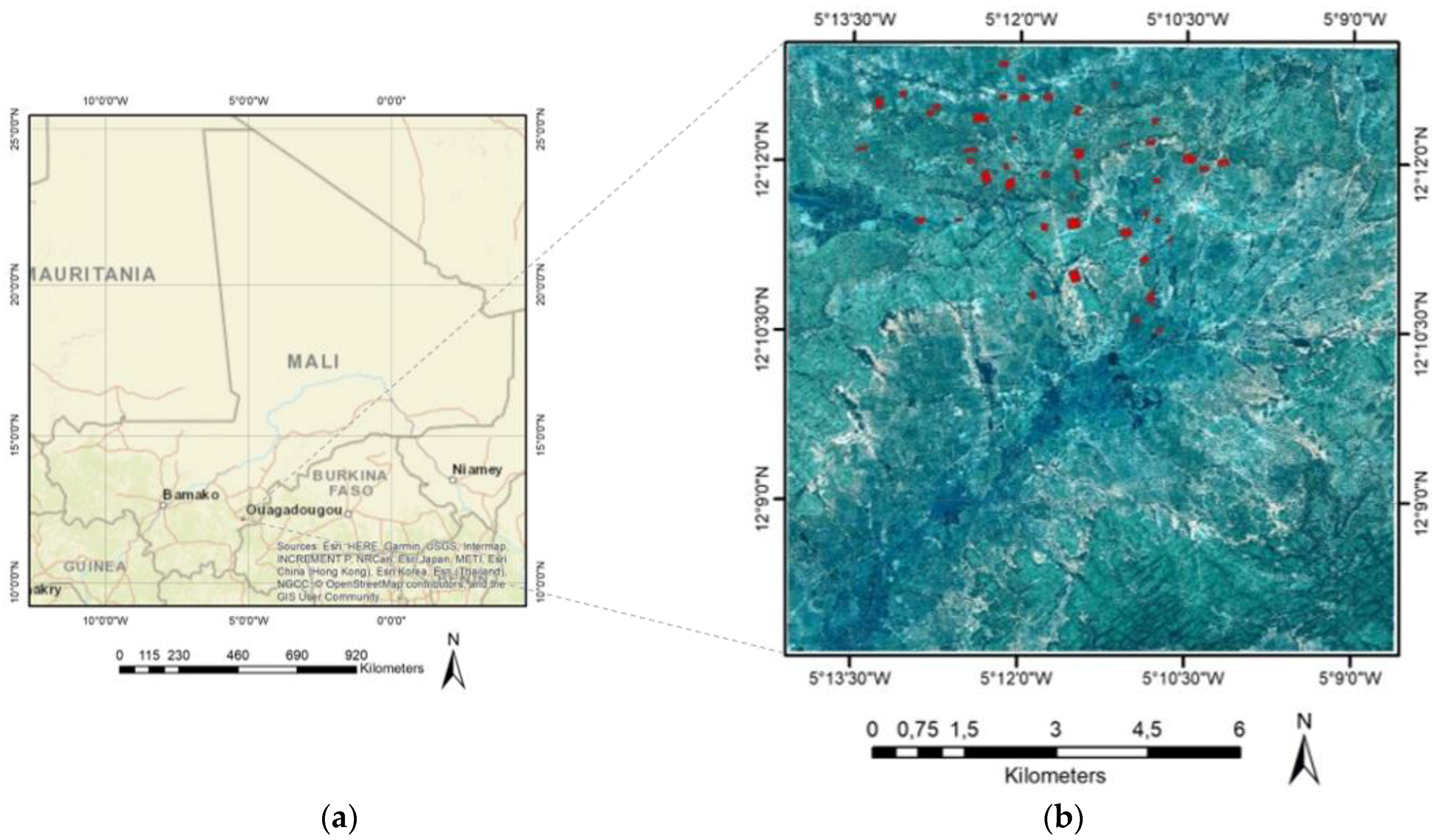
2.1. Study Area and Data

The study area covers a square of 10 × 10 km located near Koutiala, southern Mali, West Africa. This site is also an ICRISAT-led site contributing to the Joint Experiment for Crop Assessment and Monitoring (JECAM) [42]. For this area, a time series of seven multi-spectral Worldview-2 images was acquired for the cropping season of 2014. Acquisition dates of the images range from May to November covering both the beginning and the end of the crop growing season [42]. The exact acquisition dates are: 22 May, 30 May, 26 June, 29 July, 18 October, 1 November, and 14 November. The images have a pixel size of about 2 m and contain eight spectral bands in the visible, red-edge and near-infrared part of the electromagnetic spectrum. Figure 1 illustrates the study area and a zoomed in view of the area with agricultural fields. All the images were preprocessed using the STARS project workflow which uses the 6S radiative transfer model for atmospheric correction [43]. The images were atmospherically and radiometrically corrected, co-registered, and trees and clouds were masked. Crop labels for five main crops namely maize, millet, peanut, sorghum, and cotton, were collected in the field. A total of 45 fields were labeled in situ in the study area indicated in Figure 1b. This ground truth data was used to train base classifiers and to assess the accuracy of both base classifiers and ensembles.

2.2. Methods

Figure 2 presents a high-level view of the developed workflow. First, in the data preparation step (described more fully in Section 2.2.1), we extract a suite of spatial and spectral features from the available images and select the most relevant ones for image classification. Then, multiple classifiers are trained, tested, and applied to the images (Section 2.2.2). Finally, we test various approaches to create ensembles from the available classifiers and assess their classification accuracy using an independent test set (Section 2.2.3).

2.2.1. Data Preparation

A comprehensive set of spectral and spatial features is generated from the (multi-spectral) time series of Worldview-2 images. The spectral features include the vegetation indices listed in Table 1.
Spatial features are based on the Gray Level Co-occurrence Matrix (GLCM). Fifteen features proposed by [51] and three features from [52] are derived. This selection fits with their function availability in the Google Earth Engine (GEE) [53]. Formulas of these features are shown in Table A1 and Table A2.
Textural features are calculated as the average of their values in four directions (0, 45, 90, 135), applying a window of 3 × 3 pixels to the original spectral bands of each image. This configuration corresponds to the default setup in GEE and is deemed appropriate for our study since our goal is to create an efficient ensemble and not to optimize the configuration to extract spatial features.
The extraction of spectral and spatial features, computed for each pixel, results in 140 features for a single image and in 980 features for the complete time series (Table 2). Although GEE is a scalable and cloud-based platform, a timely execution of the classifiers is not possible without reducing the number of features used. Moreover, we know and empirically see (results not shown) that many features contain similar information and are highly correlated. Thus, a guided regularized random forest (GRRF) [54] is applied to identify the most relevant features. This feature selection step helps to make our classification problem both more tractable in GEE and more interpretable. GRRF requires the optimization of two regularization parameters. The most relevant features are obtained using the criteria of gain regularized higher than zero. This optimization is done for ten subsets of training data generated by randomly splitting 2129 training samples. Each subset is fed to the GRRF to select the most relevant spectral and spatial features after optimizing the two regularization parameters. The selected features are then used to train an RF classifier using all the training samples. The best set of spatial and spectral features is determined by ranking the resulting RF classifiers according to their OA for 1258 test samples.

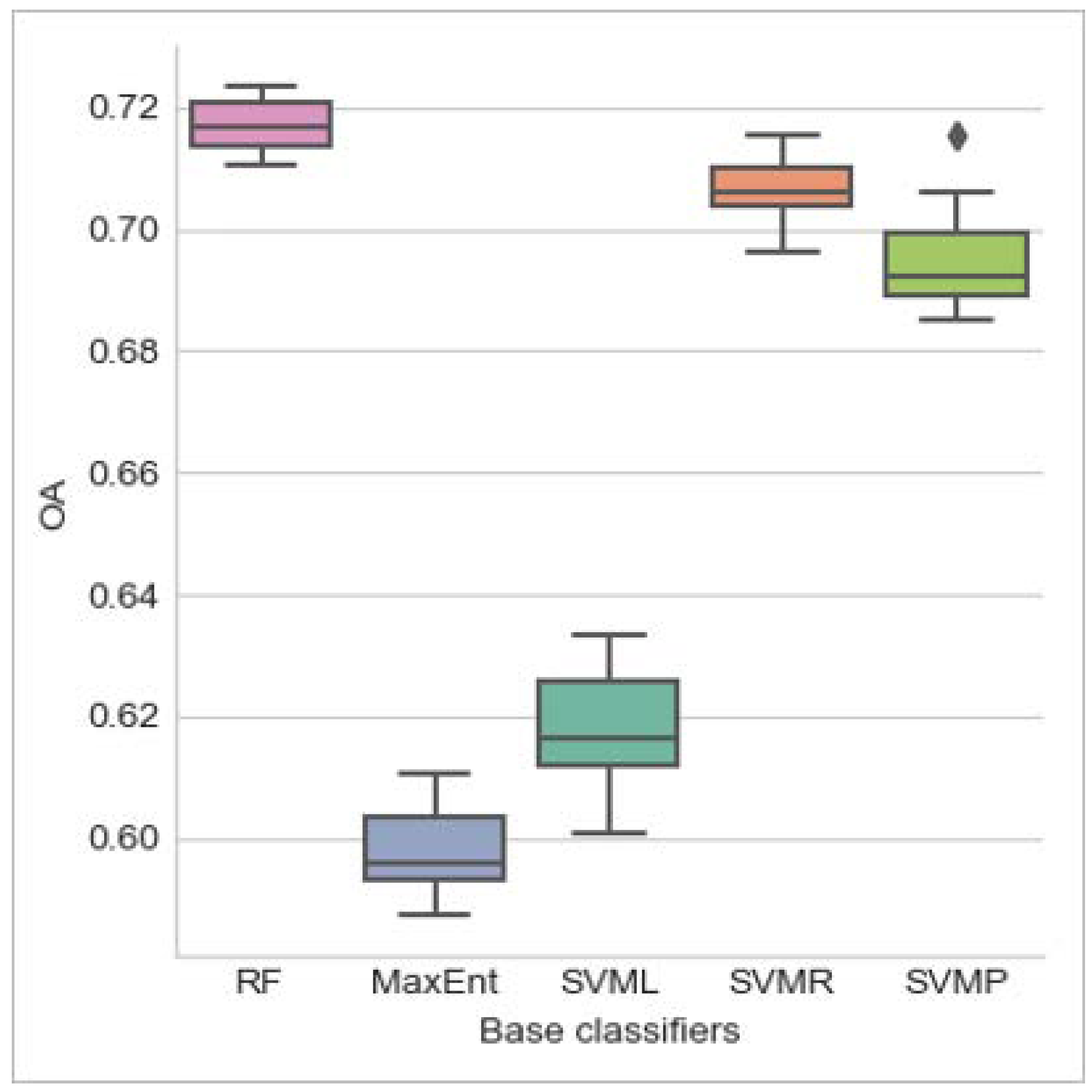
2.2.2. Base Classifiers

Several classifiers are used to create our ensembles, after performing an exploratory analysis with the available classifiers in GEE. Five classifiers are selected to create our ensembles based on their algorithmic approach and overall accuracy (OA): Random Forest (RF; [55]), Maximum Entropy Model (MaxEnt; [56]), Support Vector Machine (SVM; [57]) with linear, polynomial and Gaussian kernels. A combination with other types of classifier, e.g., a deep learning algorithm could easily be allowed when such becomes available in GEE (with inclusion of TensorFlow). This is expected to happen given the active research being performed in this field. The following paragraphs briefly describe our chosen classifiers and explain how they are used in this study.
RF is a well-known machine learning algorithm [58,59,60,61] created by combining a set of decision trees. A typical characteristic of RF is that each tree is created with a random selection of training instances and features. Once the trees are created, classification results are obtained by majority voting. RF has reached around 85% OA in crop type classification using a multi-spectral time series of RapidEye images [62], and higher than 80% for a time series of Landsat7 images in homogeneous regions [13]. RF has two user-defined parameters: the number of trees and the number of features available to build each decision tree. In our study, an RF with 300 trees is created and we set the number of features per split to the square root of the total number of features. These are standard settings [63].
MaxEnt computes an approximated probability distribution consistent with the constraints (facts) observed in the data (predictor values) and as uniform as possible [64]. This provides maximum entropy while avoiding assumptions on the unknown, hence the name of the classifier. MaxEnt was proposed to estimate geographic species distribution and potential habitat [56], to classify vegetation from remote sensing images [65], and groundwater potential mapping [66]. In our study, MaxEnt was applied with default parameter values in GEE as follows: weight for L1 regularization set to 0, weight for L2 regularization set to 0.00001, epsilon set to 0.00001, minimum number of iterations set to 0, and maximum number of iterations set to 100.
SVM is another well-known machine learning algorithm that has been widely applied for crop classification [11,67]. SVM has demonstrated its robustness to outliers and is an excellent classifier when the number of input features is high [12]. The original binary version of SVM aims to find the optimal plane that separates the available data into two classes by maximizing the distance (margins) between the so-called support vectors (i.e., the closest training samples to the optimal hyperplane). Multiple binary SVMs can be combined to tackle a multi-class problem. When the training data cannot be separated by a plane, it is mapped to a multidimensional feature space in which the samples are separated by a hyperplane. This leads to a non-linear classification algorithm that, thanks to the so-called kernel trick, only needs the definition of the dot products among the training data [68]. Linear, radial, and polynomial kernels are commonly used to define these dot products. The linear SVM only requires fixing the so-called C parameter, which represents the cost of misclassifying samples, whereas the radial and polynomial kernels require the optimization of an additional parameter, respectively called gamma and the polynomial degree. In this work, all SVM parameters were obtained by 5-fold cross validation [69], Linear kernel (SVML) was tuned in a range of initial values C = [1, 10, 50, 100, 200, 300, 400, 500, 600, 700, 800, 1000]. Gaussian kernel (SVMR) used an initial values range of C = [1, 10, 100, 200, 300] and gamma = [0.001, 0.1, 0.5, 1, 5, 10]. Also, parameters for SVM polynomial (SVMP) were tuned using C = [10, 100, 300], gamma = [0.1, 1, 10], degree = [2, 3, 4] and coef0 = [1, 10, 100].
All classifiers are trained and applied separately using a modified leave-one-out method in which the training set is stratified and randomly partitioned into k (10) equally sized subsamples. Each base classifier is trained with k − 1 subsamples, leaving one subsample out [40]. Using ten different seeds to generate the subsamples, these methods allow us to generate 100 subsets of training data that, in turn, allow 20 versions of each base classifier to be generated and a total of 100 classification models when combining the five classifiers as presented in Figure 3. This training method prevents overfitting of the base classifiers because 10% of the data is discarded each time. Overfitting prevention is desirable because the ensemble is not trainable. Metrics reported are OA and kappa coefficient. Producer accuracy (PA) per class is also computed and is used to contrast performance of individual classifiers versus ensemble classifiers.

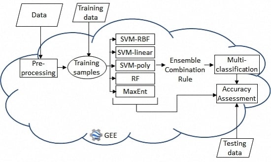
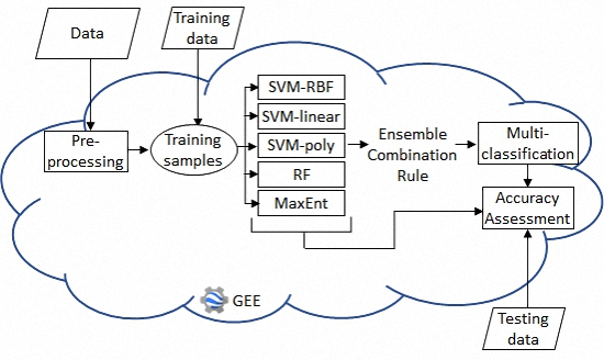
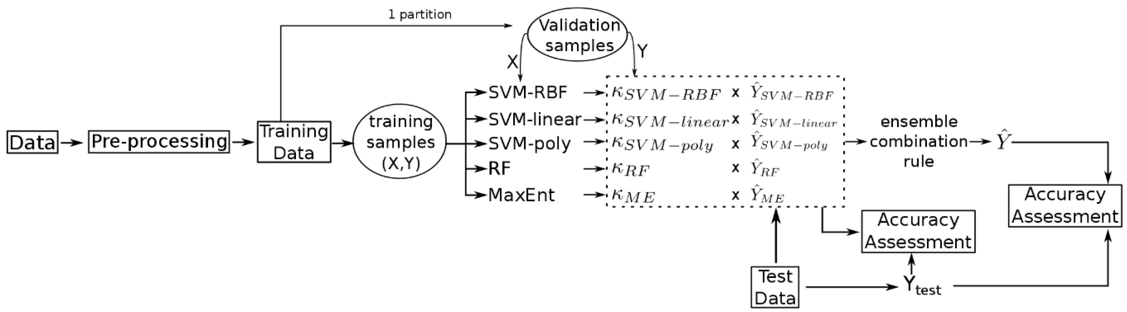
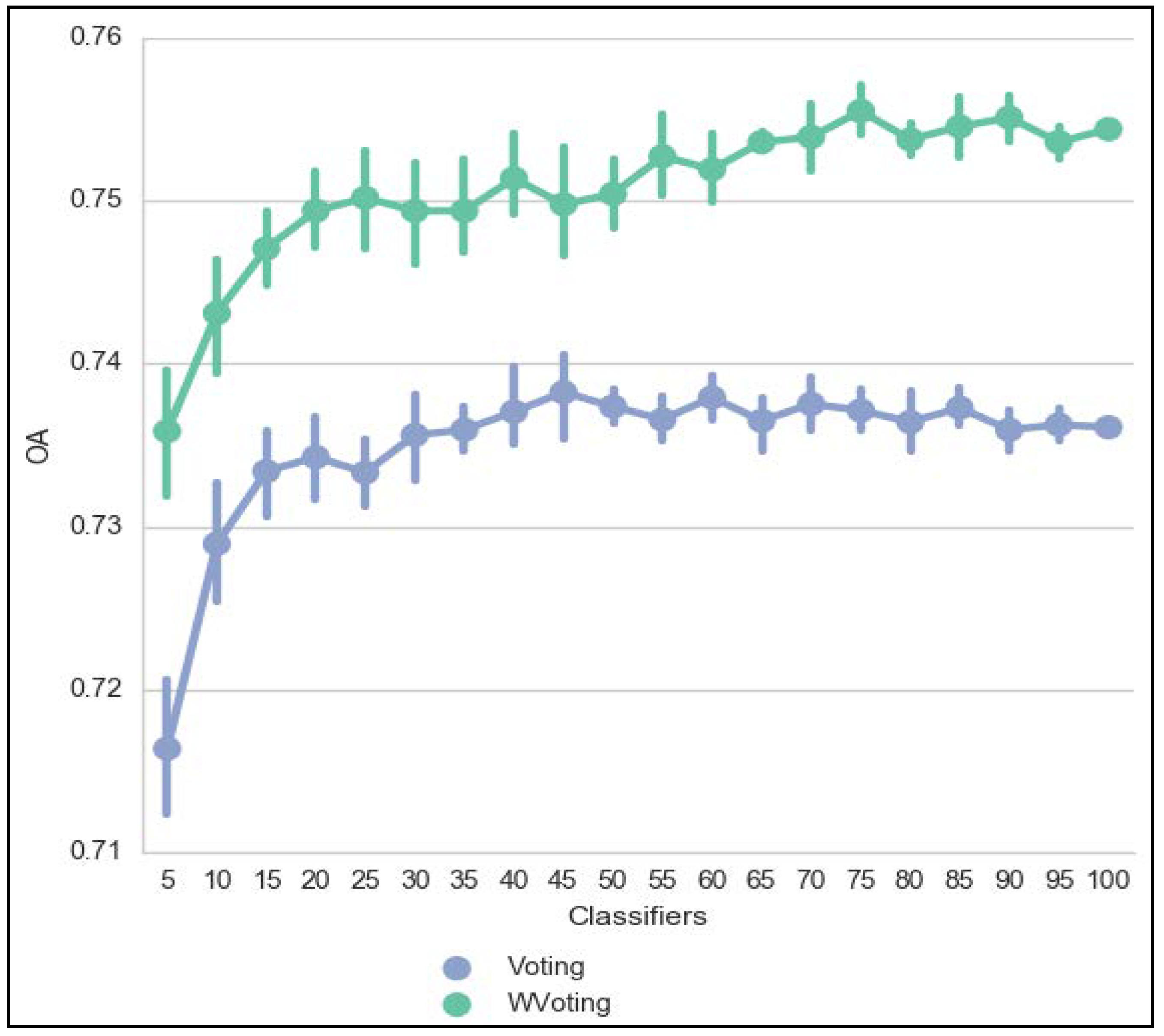
2.2.3. Ensemble Classifiers

Two combination rules, namely majority and weighted majority voting, are tested in this study to create ensemble classifiers. In the case of majority voting, the output of the ensemble is the most assigned class by classifiers, whereas in the weighted majority voting rule, a weight is assigned to each classifier to favor those classifiers with better performance in the voting decision. Both rules are easily implemented and produce results comparable to more complicated combination schemes [30,36,70]. Moreover, these rules do not require additional training data because they are not trainable [40] which means that the required parameters for the ensemble are available as the classifiers are generated and their accuracy assessed.
Majority voting works as follows. Let x denote one of the decision problem instances, let L be the number of base classifiers used, and let C be the number of possible classes. The decision (output) of classifier i on x is represented as a binary vector d x , i of the form (0, …, 0, 1, 0, …, 0), where d x , i , j = 1 if and only if the classifier labels that instance x with class C j . Further, we denote vector summation by ∑ and define the function idx@max as the index at which a maximum value is found in a vector. This function resolves ties as follow: if multiple maximal values are found, the index of the first occurrence is picked and returned. The majority voting rule of an ensemble classifier on decision problem x defines the class number D x as:
D x =   idx @ max i = 1 L d x , i ,
following [29].
Weighted majority voting is an extension of the above and uses weights w i per base classifier i.
D x = idx @ max i = 1 L w i d x , i ,
In this, we choose w i = log ( k 1 k ) , where k is the kappa coefficient of base classifier i over an independent sample set [29].
As mentioned in Section 2.2.2, our training procedure yields 20 instances of each base classifier. This allows creating two 100-classifier ensembles as well as a larger number of ensembles formed by 5, 10, 15, …, 95 classifiers. The latter ensembles serve to evaluate the impact of the size of the ensemble. To avoid biased results, we combine the base classifiers while keeping the proportion of each type of classifier. For example, the 10-classifier ensemble is created by combining two randomly chosen base classifiers of each type. This experiment means that we evaluate the classification accuracy of 191 ensembles. Classification accuracy is assessed by means of their OA, their kappa coefficient and the producer’s accuracy of each class. Besides, results of the most effective configuration of ensembles and the individual classifier with higher accuracy are compared to get insights into their performance. Examples of their output are analyzed by visual inspection.

3. Experiment Results and Discussion

3.1. Data Preparation

A feature selection method is applied before the classification to reduce the dimensionality of data without losing classification efficiency. In our study, we selected the GRRF method because it selects the features in a transparent and understandable way. The application of the GRRF to the expanded time series (i.e., the original bands plus spectral and spatial features), leads to the selection of 45 features as shown in Table 3; bands, spectral, and spatial features were selected. In general, spatial features were predominantly selected in almost all the images, whereas vegetation indices were selected in only five images. Vegetation indices have more influence when taken from images acquired when the crop has grown than when the field is bare.
A more detailed analysis of Table 3 shows that the selected multi-spectral bands and vegetation indices respectively represent 24.44% and 26.66% of the most relevant features. Textural features represent 48.88% of the most relevant features, which emphasizes the relevance of considering spatial context when analyzing very high spatial resolution images. As an example, Figure 4 and Figure 5 show the temporal evolution of a vegetation index and of one of the GLCM-based spatial features. In Figure 4, changes in TCARI are presented. Figure 4a shows a low vegetation signal since the crop is at an initial stage. In Figure 4b,c, a higher vegetation signal is shown, which relates to a more advanced growth stage. TCARI was selected for three different dates underlining the importance of changes in vegetation index for crop discrimination. Similarly, Figure 5 displays a textural feature (sum average of band 8) for a specific parcel, which points at variation in spatial patterns as the growing season goes by.

3.2. Base Classifiers and Ensembles

The accuracy of the 20 base classifiers created for each classification method is assessed using ground truth data. Table 4 lists the number of pixels per crop class used for the training and testing phase.
Figure 6 illustrates the mean performance of all base classifiers as a boxplot. The mean OA of each classifier method ranges between 59% and 72%. SVMR obtained higher accuracy than SVMP and SVML [26,71]. Lower accuracy of SVML means that linear decision boundaries are not suitable for classifying patterns in this data [72]. RF had slightly better performance than SVMR. This result is consistent with [58]. MaxEnt presented the lowest performance confirming the need for more research before it can be operationally used in multi-class classification contexts [73].
A comparison between the performance of base classifiers and ensembles was carried out. Thus, Table 5 summarizes minimum, mean, and maximum overall accuracy and kappa coefficient for both base classifiers and ensembles. We observe that ensemble classifiers in all cases outperform base classifiers with a rate of improvement ranging from 5.15% to 29.50%. On average, majority voting provides an accuracy that is 2.45% higher than that of the best base classifier (RF). Improvements are higher, at 4.65%, when a weighted voting rule is applied. This is because more effective base classifiers have more influence (weight) in the rule created to combine their outputs. Table 5 also reports associated statistics for kappa, but these values should be considered carefully [74].
The number of classifiers to build an ensemble was analyzed. In Figure 7, the mean and standard deviation of the OA is presented for each ensemble size. The weighted voting scheme outperforms the simple majority voting. The accuracy of the ensembles increases as the number of classifiers grows. However, maximum accuracy is reached when the number of classifiers is 75 for weighted voting and 45 for majority voting. This means that the majority voting approach tends to saturate with fewer classifiers than the weighted majority voting approach. The standard deviation shows a decreasing trend because as the size of the ensemble increases, results become more stable. These results are congruent with the theoretical basis of ensemble learning [29,39].
We contrast results of an ensemble sized 75 (hereafter called ensemble-75) with results obtained by an instance of RF because it had the best performance among base classifiers. Also, we compared the performance of ensemble-75 with the ensemble composed of 100 classifiers (hereafter called ensemble-100). OA for ensemble-75 is 0.7591, our chosen RF has an OA of 0.7170 and ensemble-100 has 0.7543. In Table 6, we present the confusion matrix obtained for the selected RF.
Table 7 shows the confusion matrix of the selected ensemble and in Table 8 results of applying 100 classifiers are presented.
Regarding the comparison between the performance of ensemble-75 and ensemble-100, we notice that ensemble-100 has a slightly lower OA and ensemble-75 produces better results in four of five crops. The improvement of ensemble-100 in Millet is only 0.82%, whereas there is no difference in Cotton. Sorghum, Maize, and Peanut display a lower performance with 0.43%, 2.39%, and 2.5% respectively. This means that the maximum accuracy is obtained when 75 classifiers are combined, and that addition of more classifiers does not improve the performance of ensembles.
Figure 8 presents example fields to illustrate the classification results produced by ensemble-75, ensemble-100, and the selected RF. We extracted only the fields where ground truth data was available. We observe that in both ensembles, millet is less confused with peanut and cotton than in the RF classification. Cotton is less confused with sorghum as well. Besides, confusion between maize and sorghum is lower in the ensembles than in RF. This is also true for millet. Misclassifications could obey to differences in management activities in those fields (i.e., weeding) because multiple visits by various team confirmed that a single crop was grown. Moreover, by visual analysis, it can be observed that a map produced by an ensemble seems less heterogeneous than the map produced by a base classifier (RF). Differences between maps produced by ensemble-75 and ensemble-100 are visually hardly noticeable.

4. Conclusions and Future Work

Reliable crop maps are fundamental to address current and future resource requirements. They support better agricultural management and consequently lead to enhanced food security. In a smallholder farming context, the production of reliable crop maps remains highly relevant because reported methods and techniques applied successfully to medium and lower spatial resolution images do not necessarily achieve the same success in heterogeneous environments. In this study, we introduced and tested a novel, and cloud-based ensemble method to map crops using a wide array of spectral and spatial features extracted from time series of very high spatial resolution images. The experiments carried out demonstrated the potential of ensemble classifiers to map crops grown by West African smallholders. The proposed ensemble obtained a higher overall accuracy (75.9%) than any individual classifier. This represents an improvement of 4.65% in comparison with the average overall accuracy values (71.7%) of the best base classifier tested in this study (random forest). The improvements over other tested classifiers like linear support vector machines and maximum entropy are larger, at 21.5% and 25.6% respectively. As theoretically expected, the weighted majority voting approach outperformed majority voting. A maximum performance was reached when the number of classifiers was 75. This indicates that at a certain point the addition of more classifiers does not lead to improvement of the classification results.
From a technical point of view, it is important to note that the generation of spectral and spatial features as well as the optimal use of ensemble learning, demand high computational capabilities. Today’s approaches to image processing (big data and cloud-based) allow this concern to be overcome and hold promise for practitioners (whether academic or industrial) in developing nations, as the historic setting has often confronted them with technical barriers that were hard to overcome. Data availability, computer hardware, software, or internet bandwidth have often been in the way of a more prominent uptake of remote sensing based solutions. These barriers are slowly eroding, and opportunities are arising as a consequence. In our case, GEE was helpful in providing computational capability for data preparation and allowed the systematic creation and training of up to 100 classifiers and their combinations. Further work to extend this study includes the classification of other smallholder areas in sub-Saharan African, and the addition of new images such as Sentinel-1 and -2 as time series.

Author Contributions

R.A., R.Z.-M., E.I.-V. and R.A.d.B. conceptualized the study and designed the experiments. R.A. performed the experiments, most of the analysis and prepared the first draft of the manuscript. R.Z.-M. reviewed, expanded and edited the manuscript. E.I.-V. performed the feature selection, prepared some illustrations and reviewed the manuscript. R.A.d.B. reviewed and edited the final draft of the manuscript.

Funding

This research was partially funded by Bill and Melinda Gates Foundation via the STARS Grant Agreement (1094229-2014).

Acknowledgments

We are grateful to the four reviewers for their constructive criticism on earlier drafts, which helped to improve the paper. We wish to express our gratitude to all the STARS partners and, in particular, to the ICRISAT-led team for organizing and collecting the required field data in Mali and to the STARS ITC team for pre-processing the WorldView-2 images. We express our gratitude also towards the GEE developer team for their support and timely answers to our questions.

Conflicts of Interest

The authors declare no conflict of interest.

Appendix A. Textural Features Formulas

Table A1 lists textural features from [51] with their corresponding formulas; in these, we have used the following notational conventions:
p ( i , j ) is the (i,j)th entry in a normalized gray tone matrix,
p x ( i ) = j = 1 N g P ( i , j ) is the ith entry in the marginal-probability matrix computed by summing the rows of p ( i , j )   , for fixed i,
p x ( j ) = j = 1 N g P ( i , j ) , is the jth entry in the marginal-probability matrix computed by summing the columns of p ( i , j )   , for fixed j,
N g , is the number of distinct gray levels in the quantized image,
p x + y ( k ) = i = 1 N g j = 1 N g p ( i , j ) i + j = k , and p x y ( k ) = i = 1 N g j = 1 N g p ( i , j ) | i j | = k
Table A1. Textural feature formulas from Gray Level Co-occurrence Matrix, as described in [51].
Name/FormulaName/Formula
Angular Second Moment
f 1 = i = 1 N g j = 1 N g { p ( i , j ) } 2
Contrast
f 2 = n = 0 N g 1 n 2 { i = 1 N g j = 1 N g p ( i , j ) | i j | = n }
Correlation
f 3 = i = 1 N g j = 1 N g ( i , j ) p ( i , j ) μ x μ y σ x σ y
Variance
f 4 = i = 1 N g j = 1 N g ( i μ ) 2 p ( i , j )
Inverse Difference Moment
f 5 = i = 1 N g j = 1 N g 1 1 + ( i j ) 2 p ( i , j )
Sum Average
f 6 = i = 2 2 N g i p x + y ( i )
Sum Variance
f 7 =   i = 2 2 N g     ( i f 8 ) 2 P x + y ( i )
Sum Entropy
f 8 = i = 2 2 N g p x + y ( i ) l o g { p x + y ( i ) }
Entropy
f 8 = i = 2 2 N g p x + y ( i ) l o g { p x + y ( i ) }
Difference Variance
f 10 = variance of p x y
Difference Entropy
f 11 = i = 0 N g 1 p x y ( i ) l o g { p x y ( i ) }
Information Measures of Correlation 1
f 12 = H X Y H X Y 1 m a x { H X , H Y }     where,
H X Y = i = 1 N g j = 1 N g p ( i , j ) l o g ( p ( i , j ) )
H X Y 1 = i = 1 N g j = 1 N g p ( i , j ) l o g { p x ( i ) p y ( j ) }
H X and H Y are entropies of p x and p y
Information Measures of Correlation 2
f 13 = ( 1 e [ 2.0 ( H X Y 2 H X Y ) ] ) 1 / 2 , where
H X Y 2 = i = 1 N g j = 1 N g p x ( i ) p y ( j ) log { p x ( i ) p y ( j ) }
Maximal Correlation Coefficient
f 14 = ( sec ond   largest   eigen   value   of   Q ) 1 2 where
Q ( i , j ) = k = 0 N g 1 p ( i , k ) p ( j , k ) p x ( i ) p y ( k )
Dissimilarity
f 15 = i = 1 N g j = 1 N g | i j | 2 p ( i , j )
Table A2 specifies names of the textural features proposed by [52], and their formulas, in which the following notation is used:
  s ( i , j , δ , T ) is the (i,j)th entry in a normalized gray level matrix, equivalent to p(i,j),
T represents the region and shape used to estimate the second order probabilities, and
δ = ( x , y ) is the displacement vector.
Table A2. Textural features included in the classification as described in [52].
DescriptionFormula
Inertia I ( δ , T ) = i = 0 L 1 j = 0 L 1 ( i j ) 2 s ( i , j , δ , T )
Cluster shade A ( δ , T ) = i = 0 L 1 j = 0 L 1 ( i + j μ i μ j ) 3 s ( i , j , δ , T )
Cluster prominence B ( δ , T ) = i = 0 L 1 j = 0 L 1 ( i + j μ i μ j ) 4 s ( i , j , δ , T )

References

  1. Lowder, S.K.; Skoet, J.; Singh, S. What do We Really Know about the Number and Distribution of Farms and Family Farms in the World? FAO: Rome, Italy, 2014. [Google Scholar]
  2. African Development Bank, Organisation for Economic Co-operation and Development, United Nations Development Programme. African Economic Outlook 2014: Global Value Chains and Africa’s Industrialisation; OECD Publishing: Paris, France, 2014. [Google Scholar]
  3. STARS-Project. About Us—STARS Project, 2016. Available online: http://www.stars-project.org/en/about-us/ (accessed on 1 June 2016).
  4. Haub, C.; Kaneda, T. World Population Data Sheet, 2013. Available online: http://auth.prb.org/Publications/Datasheets/2013/2013-world-population-data-sheet.aspx (accessed on 6 March 2017).
  5. Atzberger, C. Advances in Remote Sensing of Agriculture: Context Description, Existing Operational Monitoring Systems and Major Information Needs. Remote Sens. 2013, 5, 949–981. [Google Scholar] [CrossRef]
  6. Wu, B.; Meng, J.; Li, Q.; Yan, N.; Du, X.; Zhang, M. Remote sensing-based global crop monitoring: Experiences with China’s CropWatch system. Int. J. Digit. Earth 2014, 113–137. [Google Scholar] [CrossRef]
  7. Khan, M.R. Crops from Space: Improved Earth Observation Capacity to Map Crop Areas and to Quantify Production; University of Twente: Enschede, The Netherlands, 2011. [Google Scholar]
  8. Debats, S.R.; Luo, D.; Estes, L.D.; Fuchs, T.J.; Caylor, K.K. A generalized computer vision approach to mapping crop fields in heterogeneous agricultural landscapes. Remote Sens. Environ. 2016, 179, 210–221. [Google Scholar] [CrossRef]
  9. Waldner, F.; Canto, G.S.; Defourny, P. Automated annual cropland mapping using knowledge-based temporal features. ISPRS J. Photogramm. Remote Sens. 2015, 110, 1–13. [Google Scholar] [CrossRef]
  10. Foody, G.M.; Mathur, A. Toward intelligent training of supervised image classifications: Directing training data acquisition for SVM classification. Remote Sens. Environ. 2004, 93, 107–117. [Google Scholar] [CrossRef]
  11. Beyer, F.; Jarmer, T.; Siegmann, B.; Fischer, P. Improved crop classification using multitemporal RapidEye data. In Proceedings of the 2015 8th International Workshop on the Analysis of Multitemporal Remote Sensing Images (Multi-Temp), Annecy, France, 22–24 July 2015; pp. 1–4. [Google Scholar]
  12. Camps-Valls, G.; Gomez-Chova, L.; Calpe-Maravilla, J.; Martin-Guerrero, J.D.; Soria-Olivas, E.; Alonso-Chorda, L.; Moreno, J. Robust support vector method for hyperspectral data classification and knowledge discovery. IEEE Trans. Geosci. Remote Sens. 2004, 42, 1530–1542. [Google Scholar] [CrossRef]
  13. Tatsumi, K.; Yamashiki, Y.; Torres, M.A.C.; Taipe, C.L.R. Crop classification of upland fields using Random forest of time-series Landsat 7 ETM+ data. Comput. Electron. Agric. 2015, 115, 171–179. [Google Scholar] [CrossRef]
  14. Yang, C.; Everitt, J.H.; Murden, D. Evaluating high resolution SPOT 5 satellite imagery for crop identification. Comput. Electron. Agric. 2011, 75, 347–354. [Google Scholar] [CrossRef]
  15. Sweeney, S.; Ruseva, T.; Estes, L.; Evans, T. Mapping Cropland in Smallholder-Dominated Savannas: Integrating Remote Sensing Techniques and Probabilistic Modeling. Remote Sens. 2015, 7, 15295–15317. [Google Scholar] [CrossRef]
  16. Lu, D.; Weng, Q. A survey of image classification methods and techniques for improving classification performance. Int. J. Remote Sens. 2007, 28, 823–870. [Google Scholar] [CrossRef]
  17. Waldner, F.; Li, W.; Weiss, M.; Demarez, V.; Morin, D.; Marais-Sicre, C.; Hagolle, O.; Baret, F.; Defourny, P. Land Cover and Crop Type Classification along the Season Based on Biophysical Variables Retrieved from Multi-Sensor High-Resolution Time Series. Remote Sens. 2015, 7, 10400–10424. [Google Scholar] [CrossRef]
  18. Jackson, R.D.; Huete, A.R. Interpreting vegetation indices. Prev. Vet. Med. 1991, 11, 185–200. [Google Scholar] [CrossRef]
  19. Peña-Barragán, J.M.; Ngugi, M.K.; Plant, R.E.; Six, J. Object-based crop identification using multiple vegetation indices, textural features and crop phenology. Remote Sens. Environ. 2011, 115, 1301–1316. [Google Scholar] [CrossRef]
  20. Rao, P.V.N.; Sai, M.V.R.S.; Sreenivas, K.; Rao, M.V.K.; Rao, B.R.M.; Dwivedi, R.S.; Venkataratnam, L. Textural analysis of IRS-1D panchromatic data for land cover classification Textural analysis of IRS-1D panchromatic data for land cover classication. Int. J. Remote Sens. 2002, 2317, 3327–3345. [Google Scholar] [CrossRef]
  21. Shaban, M.A.; Dikshit, O. Improvement of classification in urban areas by the use of textural features: The case study of Lucknow city, Uttar Pradesh. Int. J. Remote Sens. 2001, 22, 565–593. [Google Scholar] [CrossRef]
  22. Chellasamy, M.; Zielinski, R.T.; Greve, M.H. A Multievidence Approach for Crop Discrimination Using Multitemporal WorldView-2 Imagery. IEEE J. Sel. Top. Appl. Earth Obs. Remote Sens. 2014, 7, 3491–3501. [Google Scholar] [CrossRef]
  23. Hu, Q.; Wu, W.; Song, Q.; Lu, M.; Chen, D.; Yu, Q.; Tang, H. How do temporal and spectral features matter in crop classification in Heilongjiang Province, China? J. Integr. Agric. 2017, 16, 324–336. [Google Scholar] [CrossRef]
  24. Misra, G.; Kumar, A.; Patel, N.R.; Zurita-Milla, R. Mapping a Specific Crop-A Temporal Approach for Sugarcane Ratoon. J. Indian Soc. Remote Sens. 2014, 42, 325–334. [Google Scholar] [CrossRef]
  25. Khobragade, N.A.; Raghuwanshi, M.M. Contextual Soft Classification Approaches for Crops Identification Using Multi-sensory Remote Sensing Data: Machine Learning Perspective for Satellite Images. In Artificial Intelligence Perspectives and Applications; Silhavy, R., Senkerik, R., Oplatkova, Z.K., Prokopova, Z., Silhavy, P., Eds.; Springer International Publishing: Cham, Switzerland, 2015; pp. 333–346. [Google Scholar]
  26. Oommen, T.; Misra, D.; Twarakavi, N.K.C.; Prakash, A.; Sahoo, B.; Bandopadhyay, S. An Objective Analysis of Support Vector Machine Based Classification for Remote Sensing. Math Geosci. 2008, 40, 409–424. [Google Scholar] [CrossRef]
  27. Gómez, C.; White, J.C.; Wulder, M.A. Optical remotely sensed time series data for land cover classification: A review. ISPRS J. Photogramm. Remote Sens. 2016, 116, 55–72. [Google Scholar] [CrossRef]
  28. Wozniak, M.; Graña, M.; Corchado, E. A survey of multiple classifier systems as hybrid systems. Inf. Fusion 2014, 16, 3–17. [Google Scholar] [CrossRef]
  29. Kuncheva, L.I. Combining Pattern Classifiers: Methods and Algorithms; John Wiley & Sons, Inc.: Hoboken, NJ, USA, 2004. [Google Scholar]
  30. Gopinath, B.; Shanthi, N. Development of an Automated Medical Diagnosis System for Classifying Thyroid Tumor Cells using Multiple Classifier Fusion. Technol. Cancer Res. Treat. 2014, 14, 653–662. [Google Scholar] [CrossRef] [PubMed]
  31. Li, H.; Shen, F.; Shen, C.; Yang, Y.; Gao, Y. Face Recognition Using Linear Representation Ensembles. Pattern Recognit. 2016, 59, 72–87. [Google Scholar] [CrossRef]
  32. Lumini, A.; Nanni, L.; Brahnam, S. Ensemble of texture descriptors and classifiers for face recognition. Appl. Comput. Inform. 2016, 13, 79–91. [Google Scholar] [CrossRef]
  33. Clinton, N.; Yu, L.; Gong, P. Geographic stacking: Decision fusion to increase global land cover map accuracy. ISPRS J. Photogramm. Remote Sens. 2015, 103, 57–65. [Google Scholar] [CrossRef]
  34. Lijun, D.; Chuang, L. Research on remote sensing image of land cover classification based on multiple classifier combination. Wuhan Univ. J. Nat. Sci. 2011, 16, 363–368. [Google Scholar]
  35. Li, D.; Yang, F.; Wang, X. Study on Ensemble Crop Information Extraction of Remote Sensing Images Based on SVM and BPNN. J. Indian Soc. Remote Sens. 2016, 45, 229–237. [Google Scholar] [CrossRef]
  36. Du, P.; Xia, J.; Zhang, W.; Tan, K.; Liu, Y.; Liu, S. Multiple classifier system for remote sensing image classification: A review. Sensors (Basel) 2012, 12, 4764–4792. [Google Scholar] [CrossRef] [PubMed]
  37. Gargiulo, F.; Mazzariello, C.; Sansone, C. Multiple Classifier Systems: Theory, Applications and Tools. In Handbook on Neural Information Processing; Bianchini, M., Maggini, M., Jain, L.C., Eds.; Springer: Berlin/Heidelberg, Germany, 2013; Volume 49, pp. 505–525. [Google Scholar]
  38. Corrales, D.C.; Figueroa, A.; Ledezma, A.; Corrales, J.C. An Empirical Multi-classifier for Coffee Rust Detection in Colombian Crops. In Proceedings of the Computational Science and Its Applications—ICCSA 2015: 15th International Conference, Banff, AB, Canada, 22–25 June 2015; Gervasi, O., Murgante, B., Misra, S., Gavrilova, L.M., Rocha, C.A.M.A., Torre, C., Taniar, D., Apduhan, O.B., Eds.; Springer International Publishing: Cham, Switzerland, 2015; pp. 60–74. [Google Scholar]
  39. Song, X.; Pavel, M. Performance Advantage of Combined Classifiers in Multi-category Cases: An Analysis. In Proceedings of the 11th International Conference, ICONIP 2004, Calcutta, India, 22–25 November 2004; pp. 750–757. [Google Scholar]
  40. Polikar, R. Ensemble based systems in decision making. Circuits Syst. Mag. IEEE 2006, 6, 21–45. [Google Scholar] [CrossRef]
  41. Duin, R.P.W. The Combining Classifier: To Train or Not to Train? In Proceedings of the 16th International Conference on Pattern Recognition, Quebec City, QC, Canada, 11–15 August 2002.
  42. Joint Experiment for Crop Assessment and Monitoring (JECAM). Mali JECAM Study Site, Mali-Koutiala—Site Description. Available online: http://www.jecam.org/?/site-description/mali (accessed on 18 April 2018).
  43. Stratoulias, D.; de By, R.A.; Zurita-Milla, R.; Retsios, V.; Bijker, W.; Hasan, M.A.; Vermote, E. A Workflow for Automated Satellite Image Processing: From Raw VHSR Data to Object-Based Spectral Information for Smallholder Agriculture. Remote Sens. 2017, 9, 1048. [Google Scholar] [CrossRef]
  44. Rouse, W.; Haas, R.H.; Deering, D.W. Monitoring vegetation systems in the great plains with ERTS. Proc. Earth Resour. Technol. Satell. Symp. NASA 1973, 1, 309–317. [Google Scholar]
  45. Louhaichi, M.; Borman, M.M.; Johnson, D.E. Spatially located platform and aerial photography for documentation of grazing impacts on wheat. Geocarto Int. 2001, 16, 65–70. [Google Scholar] [CrossRef]
  46. Huete, A.; Didan, K.; Miura, T.; Rodriguez, E.P.; Gao, X.; Ferreira, L.G. Overview of the radiometric and biophysical performance of the MODIS vegetation indices. Remote Sens. Environ. 2002, 83, 195–213. [Google Scholar] [CrossRef]
  47. Huete, A.R. A Soil-Adjusted Vegetation Index (SAVI). Remote Sens. Environ. 1988, 25, 295–309. [Google Scholar] [CrossRef]
  48. Qi, J.; Chehbouni, A.; Huete, A.R.; Kerr, Y.H.; Sorooshian, S. A modified soil adjusted vegetation index. Remote Sens. Environ. 1994, 48, 119–126. [Google Scholar] [CrossRef]
  49. Haboudane, D.; Miller, J.R.; Tremblay, N.; Zarco-Tejada, P.J.; Dextraze, L. Integrated narrow-band vegetation indices for prediction of crop chlorophyll content for application to precision agriculture. Remote Sens. Environ. 2002, 81, 416–426. [Google Scholar] [CrossRef]
  50. Gitelson, A.A.; Kaufman, Y.J.; Stark, R.; Rundquist, D. Novel algorithms for remote estimation of vegetation fraction. Remote Sens. Environ. 2002, 80, 76–87. [Google Scholar] [CrossRef]
  51. Haralick, R.; Shanmugan, K.; Dinstein, I. Textural features for image classification. IEEE Trans. Syst. Man Cybern. 1973, 3, 610–621. [Google Scholar] [CrossRef]
  52. Conners, R.W.; Trivedi, M.M.; Harlow, C.A. Segmentation of a high-resolution urban scene using texture operators. Comput. Vis. Graph. Image Process. 1984, 25, 273–310. [Google Scholar] [CrossRef]
  53. Gorelick, N.; Hancher, M.; Dixon, M.; Ilyushchenko, S.; Thau, D.; Moore, R. Google Earth Engine: Planetary-scale geospatial analysis for everyone. Remote Sens. Environ. 2017, 202, 18–27. [Google Scholar] [CrossRef]
  54. Izquierdo-Verdiguier, E.; Zurita-Milla, R.; de By, R.A. On the use of guided regularized random forests to identify crops in smallholder farm fields. In Proceedings of the 2017 9th International Workshop on the Analysis of Multitemporal Remote Sensing Images (MultiTemp), Brugge, Belgium, 27–29 June 2017; pp. 1–3. [Google Scholar]
  55. Breiman, L. Random forests. Mach. Learn. 2001, 45, 5–32. [Google Scholar] [CrossRef]
  56. Phillips, S.J.; Anderson, R.P.; Schapire, R.E. Maximum entropy modeling of species geographic distributions. Ecol. Model. 2006, 190, 231–259. [Google Scholar] [CrossRef]
  57. Cortes, C.; Vapnik, V. Support Vector Networks. Mach. Learn. 1995, 20, 273–297. [Google Scholar] [CrossRef]
  58. Duro, D.C.; Franklin, S.E.; Dubé, M.G. A comparison of pixel-based and object-based image analysis with selected machine learning algorithms for the classification of agricultural landscapes using SPOT-5 HRG imagery. Remote Sens. Environ. 2012, 118, 259–272. [Google Scholar] [CrossRef]
  59. Gao, T.; Zhu, J.; Zheng, X.; Shang, G.; Huang, L.; Wu, S. Mapping spatial distribution of larch plantations from multi-seasonal landsat-8 OLI imagery and multi-scale textures using random forests. Remote Sens. 2015, 7, 1702–1720. [Google Scholar] [CrossRef]
  60. Pal, M. Random forest classifier for remote sensing classification. Int. J. Remote Sens. 2005, 26, 217–222. [Google Scholar] [CrossRef]
  61. Rodriguez-Galiano, V.F.; Ghimire, B.; Rogan, J.; Chica-Olmo, M.; Rigol-Sanchez, J.P. An assessment of the effectiveness of a random forest classifier for land-cover classification. ISPRS J. Photogramm. Remote Sens. 2012, 67, 93–104. [Google Scholar] [CrossRef]
  62. Nitze, I.; Schulthess, U.; Asche, H. Comparison of Machine Learning Algorithms Random Forest, Artificial Neural Network and Support Vector Machine to Maximum Likelihood for Supervised Crop Type Classification. In Proceedings of the 4th international conference on Geographic Object-Based Image Analysis (GEOBIA) Conference, Rio de Janeiro, Brazil, 7–9 May 2012; pp. 35–40. [Google Scholar]
  63. Akar, O.; Güngör, O. Integrating multiple texture methods and NDVI to the Random Forest classification algorithm to detect tea and hazelnut plantation areas in northeast Turkey. Int. J. Remote Sens. 2015, 36, 442–464. [Google Scholar] [CrossRef]
  64. Berger, A.L.; della Pietra, S.A.; della Pietra, V.J. A Maximum Entropy Approach to Natural Language Process. Comput. Linguist. 1996, 22, 39–71. [Google Scholar]
  65. Evangelista, P.H.; Stohlgren, T.J.; Morisette, J.T.; Kumar, S. Mapping Invasive Tamarisk (Tamarix): A Comparison of Single-Scene and Time-Series Analyses of Remotely Sensed Data. Remote Sens. 2009, 1, 519–533. [Google Scholar] [CrossRef]
  66. Rahmati, O.; Pourghasemi, H.R.; Melesse, A.M. Application of GIS-based data driven random forest and maximum entropy models for groundwater potential mapping: A case study at Mehran Region, Iran. Catena 2016, 137, 360–372. [Google Scholar] [CrossRef]
  67. Mountrakis, G.; Im, J.; Ogole, C. Support vector machines in remote sensing: A review. ISPRS J. Photogramm. Remote Sens. 2011, 66, 247–259. [Google Scholar] [CrossRef]
  68. Izquierdo-Verdiguier, E.; Gómez-Chova, L.; Camps-Valls, G. Kernels for Remote Sensing Image Classification. In Wiley Encyclopedia of Electrical and Electronics Engineering; John Wiley & Sons, Inc.: Hoboken, NJ, USA, 2015; pp. 1–23. [Google Scholar]
  69. Kohavi, R. A study of cross-validation and bootstrap for accuracy estimation and model selection. Int. Jt. Conf. Artif. Intell. 1995, 1137–1143. [Google Scholar]
  70. Smits, P.C. Multiple classifier systems for supervised remote sensing image classification based on dynamic classifier selection. IEEE Trans. Geosci. Remote Sens. 2002, 40, 801–813. [Google Scholar] [CrossRef]
  71. Kavzoglu, T.; Colkesen, I. A kernel functions analysis for support vector machines for land cover classification. Int. J. Appl. Earth Obs. Geoinf. 2009, 11, 352–359. [Google Scholar] [CrossRef]
  72. Hao, P.; Wang, L.; Niu, Z. Comparison of Hybrid Classifiers for Crop Classification Using Normalized Difference Vegetation Index Time Series: A Case Study for Major Crops in North Xinjiang, China. PLoS ONE 2015, 10, e0137748. [Google Scholar] [CrossRef] [PubMed]
  73. Amici, V.; Marcantonio, M.; la Porta, N.; Rocchini, D. A multi-temporal approach in MaxEnt modelling: A new frontier for land use/land cover change detection. Ecol. Inform. J. 2017, 40, 40–49. [Google Scholar] [CrossRef]
  74. Gilmore, R.P., Jr.; Millones, M. Death to Kappa: Birth of quantity disagreement and allocation disagreement for accuracy assessment. Int. J. Remote Sens. 2011, 32, 4407–4429. [Google Scholar]
Figure 1. Study area. (a) Location of the study area in Mali; (b) The study’s field plots overlapping a Worldview-2 image of the study area on 18 October 2014 using natural color composite.
Remotesensing 10 00729 g001
Figure 2. Overview of the ensemble classifier system. X represents the features extracted during pre-processing, Y and Ytest represent ground truth of training and test data, Y ^ c l a s s is the prediction of a classifier and Y ^ the ensemble prediction. K c l a s s is the kappa obtained by a classifier.
Remotesensing 10 00729 g002
Figure 3. Leave-one-out strategy using ten seeds for generating 100 training datasets to train base classifiers (BC).
Remotesensing 10 00729 g003
Figure 4. Vegetation Index (TCARI) for a sample parcel. Dates are: (a) 26 June 2014; (b) 1 November 2014; and (c) 14 November 2014.
Remotesensing 10 00729 g004
Figure 5. Sum average of band 8 (b8_avg) for a sample parcel. Dates are: (a) 30 May 2014; (b) 1 November 2014.
Remotesensing 10 00729 g005
Figure 6. Boxplot of overall accuracy (OA) of base classifiers.
Remotesensing 10 00729 g006
Figure 7. Mean and standard deviation of the overall accuracy using majority voting and weighted majority voting.
Remotesensing 10 00729 g007
Figure 8. Comparison between field classifications produced by a 75-classifiers ensemble (E75), the 100-classifiers ensemble (E100), and a random forest classifier (RF). PA: Accuracy per class is listed below each crop. Mask corresponds to trees inside fields or clouds. VHR: overlapping area in a World-View2 image on 7 July 2014 using natural color composite.
Remotesensing 10 00729 g008
Table 1. Vegetation indices, formulas, and reference. WorldView-2 band names abbreviations are: R = Red, RE = Red edge, G = Green, B = Blue and NIR = Near IR-1.
Vegetation Index (VI)Formula
Normalized Difference Vegetation Index (NDVI) [44](NIRR)/(NIR + R)
Green Leaf Index (GLI) [45](2 × GRB)/(2 × G + R + B)
Enhanced Vegetation Index (EVI) [46]EVI = 2.5 × (NIRR)/(NIR +6 × R − 7.5 × B + 1)
Soil Adjusted Vegetation Index (SAVI) [47](1 + L) × (NIRR)/(NIR + R+ L), where L = 0.5
Modified Soil Adjusted Vegetation Index (MSAVI) [48] 0.5 × ( 2 × N I R + 1 ( 2 × N I R + 1 ) 2 8 × ( N I R R ) )
Transformed Chlorophyll Absorption in Reflectance Index (TCARI) [49]3 × ((RER) − 0.2 × (REG) × (RE/R))
Visible Atmospherically Resistance Index (VARI) [50](GR)/(G + RB)
Table 2. Type and number of features extracted from a single multi-spectral WorldView-2 image, and from the time series of seven images. Gray Level Co-occurrence Matrix (GLCM).
FeatureFeatures Per ImageTotal Per Image Series
Spectral bands749
Vegetation indices749
GLCM-based features applied to image bands126882
Total140980
Table 3. Guided regularized random forest (GRRF) selected features sorted by image date [b2: band 2, b3: band 3, b4: band 4, b5: band 5, b6: band 6, b7: band 7, b8: band 8, idm: inverse different moment, savg: sum average, dvar: difference variance, corr: correlation, diss: dissimilarity].
Image Date
22 May 201430 May 201426 June 201429 July 201418 October 20141 November 201414 November 2014
b3b3_savgb4_dissb3SAVIb3_dissb2
b7b5_savgb5_dvarb5_savgVARIb4_dvarb2_savg
b8b6_corrb8_entb6 b4_idmb3_dvar
b8_idmb7_idmGLIb6_corr b4_savgb8
b7_savgMSAVIb6_savg b6EVI
b8_savgTCARIb8_diss b6_savgTCARI
VARI b7_corr
b7_savg
b8_diss
b8_savg
EVI
GLI
TCARI
VARI
Table 4. Number of pixels per crop class for training base classifiers and assessing accuracy (testing).
ClassCrop Name# Pixels
TrainingTesting
1Maize395234
2Millet531309
3Peanut276168
4Sorghum472291
5Cotton455256
Total21291258
Table 5. Summary statistics for the overall accuracy and kappa coefficient of base classifiers and ensembles. Maximum Entropy Model (MaxEnt). Random Forest (RF). Support Vector Machine (SVM) with linear kernel (SVML). SVM with polynomial kernel (SVMP). SVM with Gaussian kernel (SVMR). Majority voting (Voting). Weighted majority voting (WVoting). In bold, the maximum OA (mean) and the maximum kappa (mean) for base classifiers and ensembles.
OAKappa
ClassifierMeanStdMinMaxMeanStdMinMax
Base ClassifierMaxEnt0.59750.00780.58740.61050.49130.00980.47850.5070
RF0.71720.00410.71070.72340.64120.00500.63330.6480
SVML0.61760.00950.60100.63350.51650.01190.49580.5361
SVMP0.69510.00920.68520.71540.61510.01140.60290.6401
SVMR0.70690.00480.69630.71540.62940.00580.61720.6398
EnsembleVoting0.73480.00600.70590.74640.66420.00750.62790.6788
WVoting0.75060.00600.72340.76070.68410.00760.64970.6969
Table 6. Confusion matrix applying a base RF classifier, PA: Producer accuracy per class.
MaizeMilletPeanutSorghumCottonPA
Maize14030544150.5983
Millet14239163370.7735
Peanut10171092480.6488
Sorghum18238224180.7698
Cotton13266211900.7422
Table 7. Confusion matrix applying an ensemble of 75 classifiers. PA: Producer accuracy per class.
MaizeMilletPeanutSorghumCottonPA
Maize1672333290.7137
Millet19243132860.7864
Peanut5191202130.7143
Sorghum21166230180.7904
Cotton17254151950.7617
Table 8. Confusion matrix applying an ensemble of 100 classifiers. PA: Producer accuracy per class.
MaizeMilletPeanutSorghumCottonPA
Maize1632533490.6966
Millet18245132760.7929
Peanut5211172230.6964
Sorghum22137229200.7869
Cotton18244151950.7617

