ASTER-Derived High-Resolution Ice Surface Temperature for the Arctic Coast


Unit of Arctic Sea-Ice Prediction, Korea Polar Research Institute, Incheon 21990, Korea
*
Author to whom correspondence should be addressed.
Remote Sens. 2018, 10(5), 662; https://doi.org/10.3390/rs10050662
Submission received: 28 February 2018
/
Revised: 19 April 2018
/
Accepted: 21 April 2018
/
Published: 24 April 2018
(This article belongs to the Section Ocean Remote Sensing)
Abstract
:Ice surface temperature (IST) controls the rate of sea ice growth and the heat exchange between the atmosphere and ocean. In this study, high-resolution IST using the Advanced Spaceborne Thermal Emission and Reflection radiometer (ASTER) thermal infrared region (TIR) images was retrieved to observe the thermal change of coastal sea ice. The regression coefficients of the multi-channel equation using ASTER brightness temperatures () and MODIS ISTs were derived. MODIS IST products (MOD29) were used as an in situ temperature substitute. The ASTER IST using five channels from band 10 () to band 14 () showed an RMSE of 0.746 K for the validation images on the Alaskan coast. The uncertainty of the two-channel ( and ) ASTER IST was 0.497 K, which was better than that of the five-channel. We thus concluded that the two-channel equation using ASTER and was an optimal model for the surface temperature retrieval of coastal sea ice. The two-channel ASTER IST showed similar accuracy at higher latitudes than in Alaska. Therefore, ASTER-derived IST with 90 m spatial resolution can be used to observe small-scale thermal variations on the sea ice surface along the Arctic coast.
1. Introduction
Arctic sea ice, which controls the absorption of solar radiation and the heat exchange between the atmosphere and ocean, has experienced dramatic changes accompanied by its interaction with the polar climate system [1,2,3]. Evolution study of sea ice-extent for Arctic sea ice for 35 years from 1978 to 2013 confirmed the ongoing loss of Arctic sea ice and found significant negative trends in all months, seasons, and in the annual mean [4]. The reduction of sea ice modifies the fluxes of sensible and latent heat from the surface to the atmosphere and affects cyclone development [5]. At the same time, the cyclone can exert a very large stress on the ice surface and, thus, change the distribution of sea ice dramatically. Storms in the Arctic Basin play a very important role in the thermal variations in the upper Arctic Ocean, since Arctic sea ice becomes less extensive and thinner it will be more vulnerable to intense storms [6,7]. The monitoring of coastal regions in the Arctic is of paramount importance in being able to understand these complex interactions. The morphology, stability, and duration of sea ice in the Arctic coastal region is changing, and these changes present challenges to humans and animals living on the coast. In addition, sea ice in the Arctic coast is very important from geological, biological, and industrial aspects [8,9]. In Barrow, Alaska, an integrated coastal sea ice observation system that includes satellite data, coastal radar, webcam, field data (e.g., snow depth and ice thickness) has been developed to provide useful information on sea ice conditions to the coastal community [10]. Despite the importance of coastal sea ice, there are fewer cases of integrated or continuous monitoring.
Satellite data can periodically monitor changes in coastal sea ice and polynya of polar regions. Passive microwave and optical satellite data provide information on the type, concentration, extent, and surface temperature of sea ice [11], which can compensate for insufficient field data. Among these, the ice surface temperature (IST) affects the sea ice volume growth rate by controlling the atmospheric-ocean heat exchange. Satellite-derived IST data has been used to analyze the activity and variability of coastal polynyas [12,13], which have a significant impact on greatly increasing the latent and sensible heat flux from the ocean [14]. The open water extent of the coastal polynya can be estimated by calculating the area of the satellite-derived IST pixels close to the water freezing temperature. The IST is obtained from the thermal bands of optical satellites such as the Moderate-Resolution Imaging Spectroradiometer (MODIS), the Advanced Very High Resolution Radiometer (AVHRR), and the Visible Infrared Imaging Radiometer Suite (VIIRS). In the clear sky of the Arctic, the AVHRR-derived IST accuracy (root mean square error, RMSE) was estimated at 0.3–2.1 K [15] and the MODIS-derived IST accuracy was reported at 1.3 K [16]. Key et al. showed that VIIRS IST could be estimated with an accuracy of 0.6 K when compared to aircraft data [17]. The spatial resolution of the major sensors (MODIS: 1 km, AVHRR: 1.09 km, and VIIRS: 750 m) providing the IST information is efficient for observing the entire Arctic Ocean, however, it is insufficient to monitor the thermal dynamics of coastal sea ice in detail.
The advanced spaceborne thermal emission and reflection radiometer (ASTER) with high spatial and spectral resolution in the thermal infrared region (TIR) (Table 1) has the ability to detect small thermal changes of coastal sea ice. The ASTER, however, has been mainly used for land observation, like other high-resolution multispectral sensors (e.g., Landsat); less cases have been applied for coastal sea ice. Furthermore, there is no ASTER algorithm for coastal sea ice temperature estimation. ASTER TIR data have been extensively used to estimate land surface temperature (LST) [18,19,20], and have also been used to retrieve sea surface temperature (SST) [21,22].
2. Data and Methodology
In order to develop the ASTER IST algorithm, a large amount of in situ temperature data with a wide temperature range collected at the ice surface were required. However, it is realistically difficult to obtain temperature data on the sea ice surface in the polar coast regularly (especially at various locations). The 16-day revisit time for ASTER is a limitation to discern high temporal resolution changes in IST, as opposed to VIIRS, MODIS, or AVHRR. In addition, cloud near shore can hamper the match-up between ASTER and field measurements. There may be a difference between in situ ice surface temperatures and Terra MODIS IST products (MOD 29, version 6), but we have used MOD 29 as a substitute for field data in view of realistic constraints. The MOD29 data with 1 km resolution are produced by the split window technique using the brightness temperature of band 31 and band 32 (Table 1). More information can be found in Hall et al. [16]. Under a clear sky condition during the cold period, the RMSE of MODIS IST was reported as 1.3 K [16]. As this was the error of the total northern hemisphere, we assessed the accuracy of the MODIS IST products on the Alaskan coast through a comparison with the near-surface air temperature from the tide stations (Prudhoe Bay, Nome, and Red Dog Dock) (Figure 1). More details are given in Section 3.1.
ASTER and MODIS on board the same Terra platform acquire data almost simultaneously. This feature provides the opportunity to complement each other in terms of temporal and spatial limitations [24]. ASTER consists of three visible and near infrared (VNIR) bands, six shortwave infrared (SWIR) bands (no longer available due to a sensor trouble after April 2008), and five TIR bands, each with a spatial resolution of 15 m, 30 m, and 90 m, respectively. In this study, we used 17 ASTER scenes for the development of the IST algorithm and seven ASTER scenes to evaluate the algorithm (Table 2). Figure 2 shows an example of an ASTER image near the Red Dog Dock for the development of the algorithm.
To develop an accurate ASTER IST algorithm, it was necessary to remove the cloud and sea water pixels in the image. To do so, first, ASTER VNIR and SWIR bands were converted to top of atmosphere (TOA) reflectance by the following equation [25]:
where is the at-sensor registered radiance for band ; is the mean solar exoatmospheric irradiance of each band ; is the earth-sun distance in astronomical units; and is the solar zenith angle. Due to the similar reflectance characteristics of clouds and sea ice at the visible wavelengths, it causes difficulties when masking the clouds from the image. Clouds generally have a higher reflectance than sea ice or snow at around 1.6 μm. This feature is useful for masking clouds in polar regions [26]. Since ASTER has an SWIR band 4 (1.6–1.7 μm), we used a TOA band ratio of < 0.17 to eliminate the cloud pixels. The band ratio using SWIR band 4 and VNIR band 3 did not identify the small size cloud and fog seen in the ASTER image. We, therefore, removed it through additional visual inspection. Sea water reflectance was significantly lower than snow or ice at the VNIR wavelength. The pixel values with a reflectance of less than 20% in band 3 were eliminated as seawater ( < 0.2).
The ASTER TIR bands were converted to the brightness temperature () by the following equation [19]:
where is the at-sensor brightness temperature for band ; is the at-sensor registered radiance for band ; and with and as the radiation constants; and is the effective wavelength. and can be read in Jimenez-Munoz and Sobrino [19].
A MODIS IST pixel (1 km) defined as sea ice through flag masking (land, ocean, and cloud) corresponded to about 121 pixels of ASTER (90 m). The 121 ASTER pixels were not uniform in a MODIS pixel as the condition of sea ice is not homogeneous. In particular, near-shore sea ice is decomposed or thin (Figure 2A). This means that the temperature of the sea ice can be influenced by the sea water below the sea ice (Figure 2B). Melt ponds on the sea ice also affect temperature. For the ASTER-MODIS match-up, the standard deviations (SD) of ASTER s corresponding to MODIS IST pixels were calculated to find MODIS pixels representing homogeneous sea ice. This was based on the assumption that a small variation of ASTER in a MODIS pixel may be due to homogeneous condition [22]. The homogeneous MODIS pixels were used as true temperature data for the development of the ASTER IST algorithm.
The surface temperature retrieval algorithm is generally developed by linking the brightness temperatures of the satellite sensor with in situ surface measurements. A linear split window technique first proposed by McMillin [27] corrected the atmospheric attenuation of upwelling radiation due to water vapor absorption using the difference in brightness temperature between the two infrared bands at 11–12 μm [28]. This method was commonly used for SST and IST retrievals [15,16,29,30]. A general linear multi-channel algorithm can be written as [23]:
where is the temperature of sea or ice surface; . and are scan angle-dependent coefficients; and are the brightness temperatures of each band of . The coefficients were determined through a least squares regression procedure, where surface temperatures were regressed against brightness temperatures. Brightness temperature differences between two bands may also be used.
3. Results
3.1. Comparison MOD29 IST to Near-Surface Air Temperature
In order to validate the accuracy of the MODIS IST product as a substitute for field measurement, MOD29 products and near-surface air temperatures were compared. The near-surface air temperatures from the Prudhoe Bay (sensor height, 4 m), Nome (sensor height, 4 m), and Red Dog Dock (sensor height, 9 m) tide stations operated by NOAA were used (Figure 1). There were 175 cases where the surface temperature data and the MODIS IST were matched within 30 min from 2005 to 2016 (March and April). The MODIS IST pixel nearest to the station was used for validation. The validation indicated that the MOD29 had a bias of −1.98 K and RMSE of 3.1 K (Figure 3). This difference is generally known to be due to long-wave radiative cooling under a cloud free-sky during the winter season [16,31,32]. According to the measurements of the Surface Heat Budget of the Arctic Ocean Experiment (SHEBA), the daily surface temperatures could be as much as 5 K lower than at the 10-m height [32]. In the Antarctic Remote Ice Sensing Experiment (ARISE), the difference between the ice surface skin temperature and air temperature at 21-m height ranged from 2 to 15 K [33]. Considering the atmospheric thermal inversions, when we subtracted the bias from each near-surface air temperature and recalculated, the adjusted RMSE of MOD 29 was 2.39 K in the Alaskan coast.
The MODIS IST accuracy for the Alaskan coast was not significantly different from those (RMSE of 1–3 K) estimated in previous studies for the polar region. Hall et al. [9] showed that during the cold period in the Arctic Ocean, the MODIS IST bias, which utilizes the MODIS cloud mask, was −2.1 K and with the bias removed, the RMSE was 3.0 K. Scambos et al. [33] observed an uncertainty of 1 K through comparing MODIS IST with ship-borne sea-ice skin temperature from the sea ice zone off East Antarctic. The difference of error between these studies was due to the variability of ice surface temperature depending on cloud, humidity, and wind conditions. For example, the difference between air temperature and surface temperature can be reduced as atmospheric mixing occurs near the surface as wind speed increases [9]. In our experiment, when the wind speed was more than 10 m/s (N = 30), the RMSE decreased to 1.38 K. With speed less than 10 m/s (N = 126), the RMSE increased to 2.52 K.
3.2. ASTER IST Algorithm
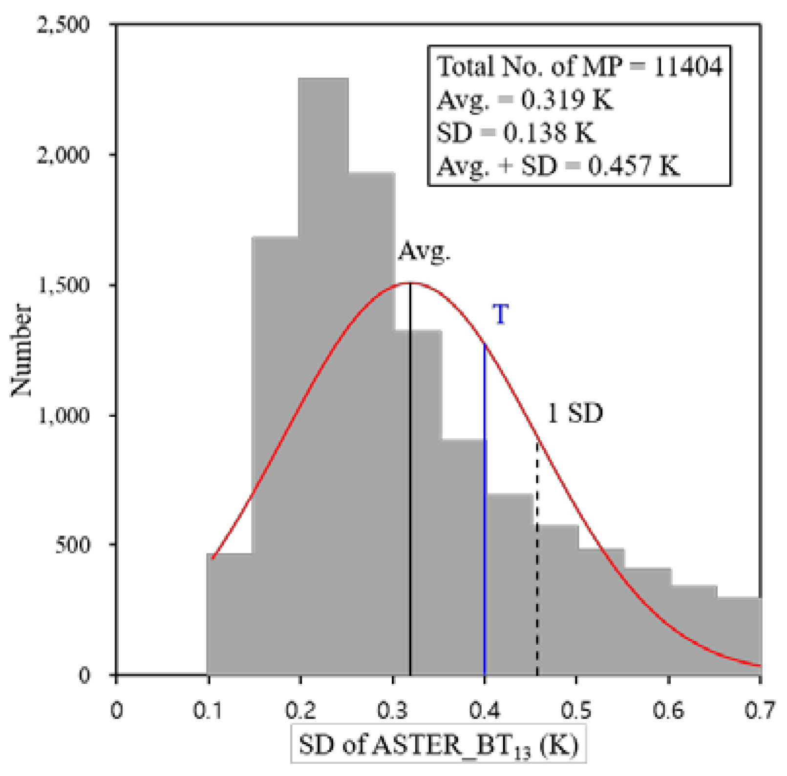
In order to develop an accurate ASTER IST algorithm, MODIS IST pixels representing homogeneous sea ice should be used as the true temperature data. MODIS IST pixels representing homogeneous sea ice were determined by following several steps. First, as a MODIS pixel (1 km) corresponds to about 121 ASTER (90 m) pixels, if the number of ASTER pixels was less than 121, the MODIS pixels were determined to be pixels influenced by sea water or cloud and were excluded from the analysis. In the next step, the SD of the ASTER pixels in a MODIS pixel were calculated. We judged the MODIS pixels with a SD of ASTER of greater than 0.7 K to have an inhomogeneous sea ice condition. A histogram of MODIS pixels (N = 11,404) with a SD of less than 0.7 K for 17 ASTER scenes used for algorithm development (Table 2) is shown in Figure 4 and roughly followed a Gaussian distribution. The average of the fitted Gaussian distribution was 0.319 K, the SD of that was 0.138 K, and the average plus the SD was 0.527 K. We assumed that MODIS IST pixels with a SD of ASTER of less than 0.4 K represented a relatively homogeneous sea ice condition. The 7938 MODIS pixels were used as the true temperature for ASTER IST algorithm development (Table 2). The MODIS IST pixels with a SD of greater than 0.4 K were generally sea ice with cracks or melt ponds.
To select the appropriate multi channels for use in the development of the split window algorithm for the ASTER IST retrieval, we compared the brightness temperatures of the five ASTER TIR bands with the 7938 MODIS IST pixels (Figure 5). The best correlation was found in ASTER , with a bias of 0.031 K and a RMSE of 0.515 K (Table 3). ASTER showed the second best correlation with a bias of −0.402 K and a RMSE of 0.678 K. This is because the wavelengths of the ASTER and are similar to the wavelengths of the MODIS band 31 and 32 used in the split window technique of the MODIS IST product (Table 1). Even before the atmospheric effect was removed, the total bias (>240 K) between the ASTER and the MODIS IST was small (0.031 K). However, when the range of brightness temperatures was divided, the results showed a bias of 0.17 K at below 260 K and −0.12 K at above 260 K. The bias at low temperatures was associated with long-wave radiative cooling and the bias at high temperatures appeared to be due to the atmospheric effect.
We derived the regression coefficient of Equation (4) using the MODIS IST and the ASTER two channels ( and ) (Table 4):
where is the ASTER IST; , , and . are regression coefficients; and and are the brightness temperatures at ASTER bands 13 and 14. In this equation, the satellite scan angle term was not considered. Since ASTER has a small scan angle with a narrow swath, the dependence on scan angle in a split window algorithm can be ignored [22]. The regression coefficients for 17 ASTER scenes used for algorithm development were derived for the following temperature ranges: > 240 K, 240 K < < 260 K, and > 260 K (Table 4). There was no significant difference in ASTER IST retrieval accuracy between the results of applying the all range ( > 240 K) coefficients and the divided range (240 K < < 260 K, > 260 K) coefficients (Table 5). Figure 6A shows the relationship between ASTER IST retrieved from Equation (4), which used the divided range coefficients, and MODIS IST. The bias was 0 K because it was adjusted statistically, and the uncertainty (RMSE) was 0.469 K. As the atmospheric effect and long-wave radiative cooling were corrected, the slope became closer to 1. The validation of the 2-channel ( and ) ASTER IST for seven validation images (Table 2) showed a 0.168 K bias and 0.497 K uncertainty (Figure 6B). This result shows that ASTER IST can provide accuracy in sea ice surface temperatures as much as the MODIS IST product.
Matsuoka et al. [22] showed that multiple regression equation using five TIR bands of ASTER was the most accurate for SST estimation. Using five TIR bands ( to ), the five-channel ASTER IST equation is expressed as follows:
where is the ASTER IST; , , , , , and are regression coefficients (Table 4); and to are the brightness temperatures at ASTER bands 10 to 14. At the five-channel ASTER IST for 17 ASTER scenes used for algorithm development, the bias and uncertainty were slightly less than the two-channel IST (Table 5). However, the bias and uncertainty of the five-channel IST for the seven validation images were considerably higher than that of the two-channel IST. Considering the above results, we concluded that the ASTER IST retrieval using two bands ( and ) and the divided range coefficients (240 K < < 260 K, > 260 K) was suitable for Alaskan coastal sea ice.
Figure 7B shows the ASTER IST image generated using the two-channel algorithm of Equation (4) and the divided range coefficients are presented in Table 4. The image displays the temperature variations of the thin sea ice near the coast in detail, which were difficult to identify in the MODIS IST image with 1 km resolution (Figure 7A). The ASTER IST image also clearly revealed the thermal differences (yellow and red colors in Figure 7B) between the ice crevices in the thick ice layers (blue colors in Figure 7B) far from the coast than MODIS IST.
4. Discussion
The satellite-derived ISTs were obtained in the clear skies where pixels affected by clouds were removed through cloud masking procedures. However, similar reflectance characteristics of clouds and sea ice at visible wavelengths made it difficult to remove small clouds and fog completely. In addition, the saturation was found in the VNIR bands of some ASTER Polar images, and the use of SWIR bands was impossible after April 2008. As a result, cloud masking using ASTER VNIR and SWIR bands has limitations. Improved cloud masking techniques for the polar environment are required to separate thin clouds and fog and their shadows from sea ice. A cloud masking algorithm, such as that using neural networks reported by Mclntire and Simpson [26], may be useful in polar regions. This will improve the accuracy of satellite-derived IST.
ASTER and MODIS sensors on board the same satellite platform acquire data at the same elevation and coincident nadirs. Simultaneous observations have the advantage of reducing the difference between the two sensors due to the time difference. There have been studies to directly compare temperatures derived from two sensors due to this feature. The validation of ASTER LST products against the MODIS LST products on ice and snow surface over Greenland were reported to have a 0.22 °C bias and 0.54 °C RMSE [34]. The result of the ASTER-derived SST validation using MODIS-derived SST for Sendai Bay, Japan showed that the bias was 0.10 °C and RMSE was 0.46 °C [15]. In this study, ASTER-derived ISTs had a mean 0.168 K higher than MODIS IST products and showed an RMSE of 0.497 K. The difference between ASTER and MODIS was highest in LST, intermediate in IST, and lowest in SST. This is related to the variability of surface conditions. LST estimates are generally known to be less accurate than SST estimates due to the large variability of surface conditions [35]. As a result, the larger the variability of the surface condition, the larger the temperature difference between the ASTER and MODIS.
A key question is whether the ASTER two-channel regression coefficients derived from Alaskan coasts can be used for higher-latitude coastal sea ice temperature retrieval. We tested the performance of the two-channel ASTER IST algorithm in some high-latitudes, including the Greenland coasts, the Laptev coastal sea, and the Canadian Archipelago. The cloud-free ASTER images were used and the MODIS IST range was 250–270 K. The validation of ASTER-retrieved IST showed a bias of 0.182 K and a RMSE of 0.488 K, which was similar to the validation result on the Alaskan coast (bias: 0.168 K and RMSE: 0.497 K).
5. Conclusions
A high-resolution retrieval IST algorithm from ASTER TIR images for Arctic coast sea ice was presented. Due to the difficulty of continuous field measurements on the sea ice surface, the MODIS IST image near the three Alaskan tide stations were used as true data. The bias between MODIS IST products and near-surface air temperatures was −1.98 K and the RMSE was 2.39 K, where the negative bias meant that the MODIS IST was lower than the near-surface air temperatures. Considering the long-wave radiative cooling effect under a cloud free-sky during the winter season, the MODIS IST bias and uncertainty may actually be smaller. In addition, since near-surface air temperature data are recorded at one point and a MODIS pixel recorded for the 1 km area, the near-surface air temperature data may often not be representative of a pixel [34].
The five-channel ASTER IST algorithm showed an RMSE of 0.746 K for the validation images. The uncertainty of the two-channel ASTER IST algorithm was 0.497 K, which was better than the five-channel algorithm. In fact, it is difficult to say that, in almost all cases, the RMSE of the two-channel algorithm is lower than five-channel algorithm. This is because we did not evaluate every Arctic coast. However, we have confirmed that at higher latitudes such as Greenland coasts, Laptev coastal sea, and Canadian Archipelago the two-channel algorithm was more accurate than five-channel algorithm and the two-channel ASTER IST coefficients could be used well. We, thus, concluded that the two-channel ASTER IST algorithm was an optimal model for surface temperature retrieval of coastal sea ice in Arctic in the 240–270 K range.
The ASTER ISTs first developed in this study are the highest resolution spatial information that can be acquired via current satellites. ASTER-derived high resolution IST can be used instead of the low-resolution MODIS IST product to observe small-scale thermal variations on sea ice surface in the Arctic coast, and may aid understanding in the interaction between ice, polynya, ocean, and atmosphere. In addition, it can be used as ancillary data for studies on growth, morphology, safety, and the dynamics of coastal sea ice that affect human activity.
Author Contributions
Young-Sun Son conceived and designed the study, performed the experiments, analyzed the results, and wrote the manuscript. Hyun-cheol Kim contributed to the research design, and provided analysis tools and constructive comments on the whole manuscript. Sung Jae Lee contributed to the experiments.
Acknowledgments
This study was supported by the Korea Polar Research Institute (KOPRI) grant PE18120 (research on analytical techniques for satellite observation of Arctic sea ice).
Conflicts of Interest
The authors declare no conflict of interest.
References
- Serreze, M.C.; Stroeve, J. Arctic sea ice trends, variability and implications for seasonal ice forecasting. Philos. Trans. R. Soc. A 2015, 373, 20140159. [Google Scholar] [CrossRef] [PubMed]
- Schweiger, A.J.; Lindsay, R.W.; Vavrus, S.; Francis, J.A. Relationships between Arctic sea ice and clouds during autumn. J. Clim. 2008, 21, 4799–4810. [Google Scholar] [CrossRef]
- Taylor, P.C.; Kato, S.; Xu, K.-M.; Cai, M. Covariance between Arctic sea ice and clouds within atmospheric state regimes at the satellite footprint level. J. Geophys. Res. Atmos. 2015, 120, 12656–12678. [Google Scholar] [CrossRef] [PubMed]
- Simmonds, I. Comparing and contrasting the behaviour of Arctic and Antarctic sea ice over the 35 year period 1979–2013. Ann. Glaciol. 2015, 56, 18–28. [Google Scholar] [CrossRef]
- Murray, R.J.; Simmonds, I. Responses of climate and cyclones to reductions in Arctic winter sea ice. J. Geophys. Res. Ocean. 1995, 100, 4791–4806. [Google Scholar] [CrossRef]
- Simmonds, I.; Burke, C.; Keay, K. Arctic Climate Change as Manifest in Cyclone Behavior. J. Clim. 2008, 21, 5777–5796. [Google Scholar] [CrossRef]
- Blunden, J.; Arndt, D.S. State of the climate in 2012. Bull. Am. Meteorol. Soc. 2013, 94, S1–S258. [Google Scholar] [CrossRef]
- Barnhart, K.R.; Overeem, I.; Anderson, R.S. The effect of changing sea ice on the physical vulnerability of Arctic coasts. Cryosphere 2014, 8, 1777–1799. [Google Scholar] [CrossRef]
- Meier, W.N.; Hovelsrud, G.K.; van Oort, B.E.; Key, J.R.; Kovacs, K.M.; Michel, C.; Haas, C.; Granskog, M.A.; Gerland, S.; Perovich, D.K.; et al. Arctic sea ice in transformation: A review of recent observed changes and impacts on biology and human activity. Rev. Geophys. 2014, 52, 185–217. [Google Scholar] [CrossRef]
- Druckenmiller, M.L.; Eicken, H.; Johnson, M.; Pringle, D.; Williams, C. Towards an integrated coastal sea-ice observatory: System components and a case study at Barrow, Alaska. Cold Reg. Sci. Technol. 2009, 56, 61–72. [Google Scholar] [CrossRef]
- Liu, Y.; Key, J.; Mahoney, R. Sea and freshwater ice concentration from VIIRS on suomi NPP and the future JPSS satellites. Remote Sens. 2016, 8, 523. [Google Scholar] [CrossRef]
- Ciappa, A.; Pietranera, L.; Budillon, G. Observations of the Terra Nova Bay (Antarctica) polynya by MODIS ice surface temperature imagery from 2005 to 2010. Remote Sens. Environ. 2012, 119, 158–172. [Google Scholar] [CrossRef]
- Aulicino, G.; Sansiviero, M.; Paul, S.; Cesarano, C.; Fusco, G.; Wadhams, P.; Budillon, G. A new approach for monitoring the Terra Nova Bay polynya through MODIS ice surface temperature imagery and its validation during 2010 and 2011 winter seasons. Remote Sens. 2018, 10, 366. [Google Scholar] [CrossRef]
- Hirano, D.; Fukamachi, Y.; Watanabe, E.; Ohshima, K.I.; Iwamoto, K.; Mahoney, A.R.; Eicken, H.; Simizu, D.; Tamura, T. A wind-driven, hybrid latent and sensible heat coastal polynya off Barrow, Alaska. J. Geophys. Res. Ocean. 2016, 121, 980–997. [Google Scholar] [CrossRef]
- Key, J.R.; Collins, J.B.; Fowler, C.; Stone, R.S. High latitude surface temperature estimates from thermal satellite data. Remote Sens. Environ. 1997, 61, 302–309. [Google Scholar] [CrossRef]
- Hall, D.; Key, J.; Casey, K.; Riggs, G.; Cavalieri, D. Sea ice surface temperature product from MODIS. IEEE Trans. Geosci. Remote Sens. 2004, 42, 1076–1087. [Google Scholar] [CrossRef]
- Key, J.; Mahoney, R.; Liu, Y.; Romanov, P.; Tschudi, M.; Appel, I.; Maslanik, J.; Baldwin, D.; Wang, X.; Meade, P. Snow and ice products from Suomi NPP VIIRS. J. Geophys. Res. Atmos. 2013, 118, 12816–12830. [Google Scholar] [CrossRef]
- Gillespie, A.; Rokugawa, S.; Matsunaga, J.S.; Cothern, S.; Kahle, A.B. Temperature and emissivity separation algorithm for Advanced Spaceborne Thermal Emission and Reflection Radiometer (ASTER) images. IEEE Trans. Geosci. Remote Sens. 1998, 36, 1113–1126. [Google Scholar] [CrossRef]
- Jimenez-Munoz, J.C.; Sobrino, J.A. Feasibility of retrieving land-surface temperature from ASTER TIR bands using two-channel algorithms: A case study of agricultural areas. IEEE Geosci. Remote Sens. Lett. 2007, 4, 60–64. [Google Scholar] [CrossRef]
- Wang, K.; Liang, S. Evaluation of ASTER and MODIS land surface temperature and emissivity products using long-term surface longwave radiation observations at SURFRAD sites. Remote Sens. Environ. 2009, 113, 1556–1565. [Google Scholar] [CrossRef]
- Tonooka, H.; Palluconi, F. Validation of ASTER/TIR standard atmospheric correction using water surfaces. IEEE Trans. Geosci. Remote Sens. 2005, 43, 2769–2777. [Google Scholar] [CrossRef]
- Matsuoka, Y.; Kawamura, H.; Sakaida, F.; Hosoda, K. Retrieval of high-resolution sea surface temperature data for Sendai Bay, Japan, using the advanced spaceborne thermal emission and reflection radiometer (ASTER). Remote Sens. Environ. 2011, 115, 205–213. [Google Scholar] [CrossRef]
- Key, J.; Haefliger, M. Arctic ice surface-temperature retrieval from AVHRR thermal channels. J. Geophys. Res. Atmos. 1992, 97, 5885–5893. [Google Scholar] [CrossRef]
- Liu, Y.; Noumi, Y.; Yamaguchi, Y. Discrepancy between ASTER- and MODIS- derived land surface temperatures: Terrain effects. Sensors 2009, 9, 1054–1066. [Google Scholar] [CrossRef] [PubMed]
- Markham, B.L.; Barker, J.L. Thematic mapper band pass solar exoatmospherical Irradiances. Int. J. Remote Sens. 1987, 8, 517–523. [Google Scholar] [CrossRef]
- McIntire, T.J.; Simpson, J.J. Arctic sea ice, cloud, water, and lead classification using neural networks and 1.6 µm data. IEEE Trans. Geosci. Remote Sens. 2002, 40, 1956–1972. [Google Scholar] [CrossRef]
- McMillin, L.M. Estimation of sea surface temperatures from two infrared window measurements with different absorption. J. Geophys. Res. 1975, 80, 5113–5117. [Google Scholar] [CrossRef]
- Barton, I.J.; Zavody, A.M.; O’Brien, D.M.; Cutten, D.R.; Saunders, R.W.; Llewellyn-Jones, D.T. Theoretical algorithms for satellite-derived sea surface temperatures. J. Geophys. Res. 1989, 94, 3365–3375. [Google Scholar] [CrossRef]
- Vincent, R.F.; Marsden, R.F.; Minnett, P.J.; Buckley, J.R. Arctic waters and marginal ice zones: 2. An investigation of arctic atmospheric infrared absorption for advanced very high resolution radiometer sea surface temperature estimates. J. Geophys. Res. 2008, 113. [Google Scholar] [CrossRef]
- Ditri, A.L.; Minnett, P.J.; Liu, Y.; Kilpatrick, K.; Kumar, A. The Accuracies of Himawari-8 and MTSAT-2 sea-surface temperatures in the tropical western Pacific Ocean. Remote Sens. 2018, 10, 212. [Google Scholar] [CrossRef]
- Jordan, R.E.; Andreas, E.L.; Makshtas, A.P. Heat budget of snow-covered sea ice at North Pole 4. J. Geophys. Res. 1999, 104, 7785–7806. [Google Scholar] [CrossRef]
- Persson, P.O.G.; Fairall, C.W.; Andreas, E.L.; Guest, P.S.; Perovich, D.K. Measurements near the atmospheric surface flux group tower at SHEBA: Near-surface conditions and surface energy budget. J. Geophys. Res. 2002, 107, 8045. [Google Scholar] [CrossRef]
- Scambos, T.A.; Haran, T.M.; Massom, R. Validation of AVHRR and MODIS ice surface temperature products using in situ radiometers. Ann. Glaciol. 2006, 44, 345–351. [Google Scholar] [CrossRef]
- Hall, D.K.; Box, J.E.; Casey, K.A.; Hook, S.J.; Shuman, C.A.; Steffen, K. Comparison of satellite-derived and in-situ observations of ice and snow surface temperatures over Greenland. Remote Sens. Environ. 2008, 112, 3739–3749. [Google Scholar] [CrossRef]
- Price, J.C. Estimating surface temperatures from satellite thermal infrared data-A simple formulation for the atmospheric effect. Remote Sens. Environ. 1983, 13, 353–361. [Google Scholar] [CrossRef]
Figure 1.
Footprints of advanced spaceborne thermal emission and reflection radiometer (ASTER) data used for IST algorithm development in the Alaskan coastal sea. The red box is the footprint of the ASTER example image near Red Dog Dock (see Figure 2).
Figure 1.
Footprints of advanced spaceborne thermal emission and reflection radiometer (ASTER) data used for IST algorithm development in the Alaskan coastal sea. The red box is the footprint of the ASTER example image near Red Dog Dock (see Figure 2).
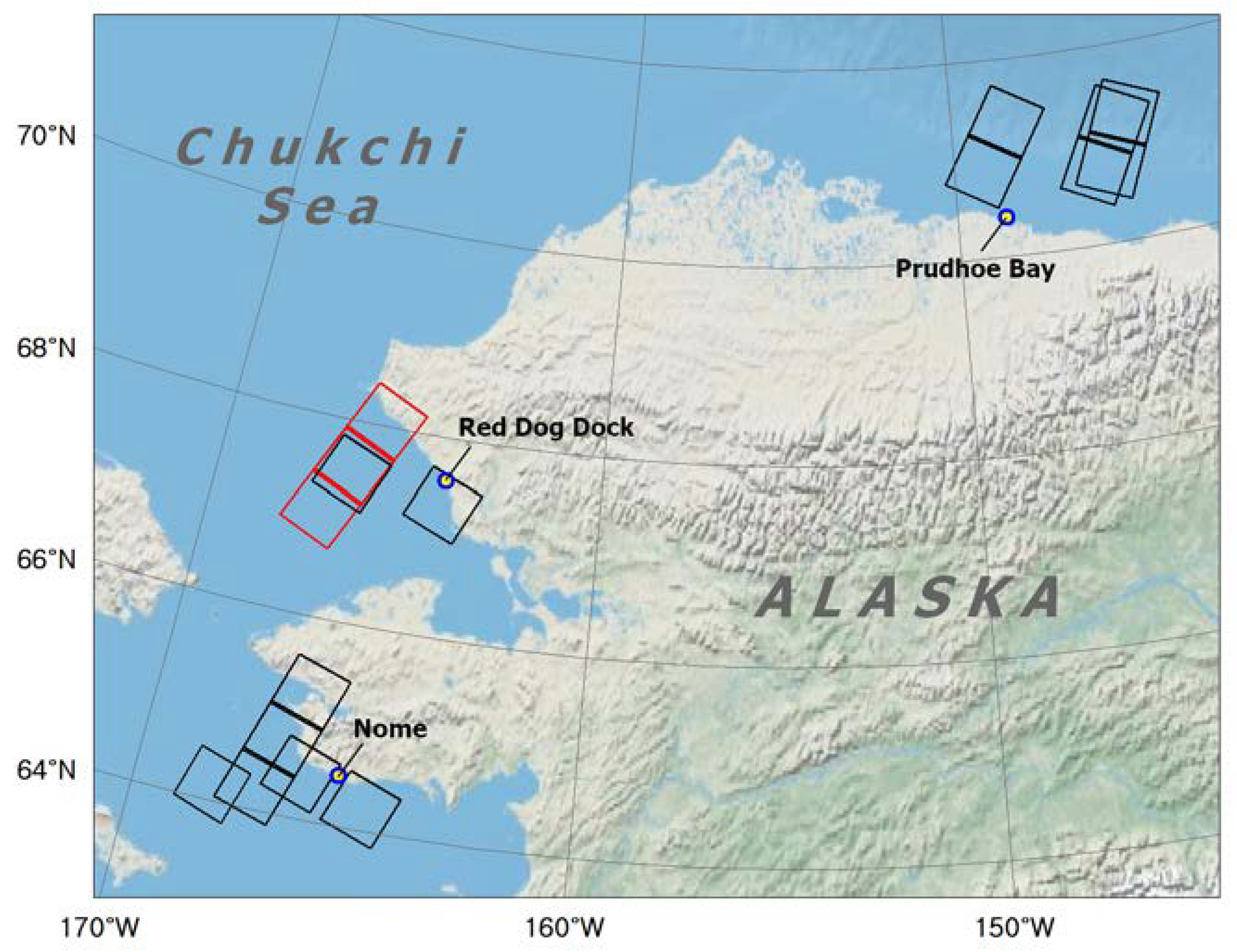
Figure 2.
ASTER RGB mosaic image acquired on 11 March 2003 near Red Dog Dock (left) including the subset image (A). The subset image shows various sea ice types near the shore line. The RGB image location is identical to the red box in Figure 1. (B) Brightness temperature image converted from ASTER TIR band 13. The temperature varies depending on the sea ice conditions. The closer to black, the lower the temperature. (C) MODIS IST image that is identical to the location of the ASTER subset image. Black pixels indicate the sea water mask. The darker the gray, the lower the temperature.
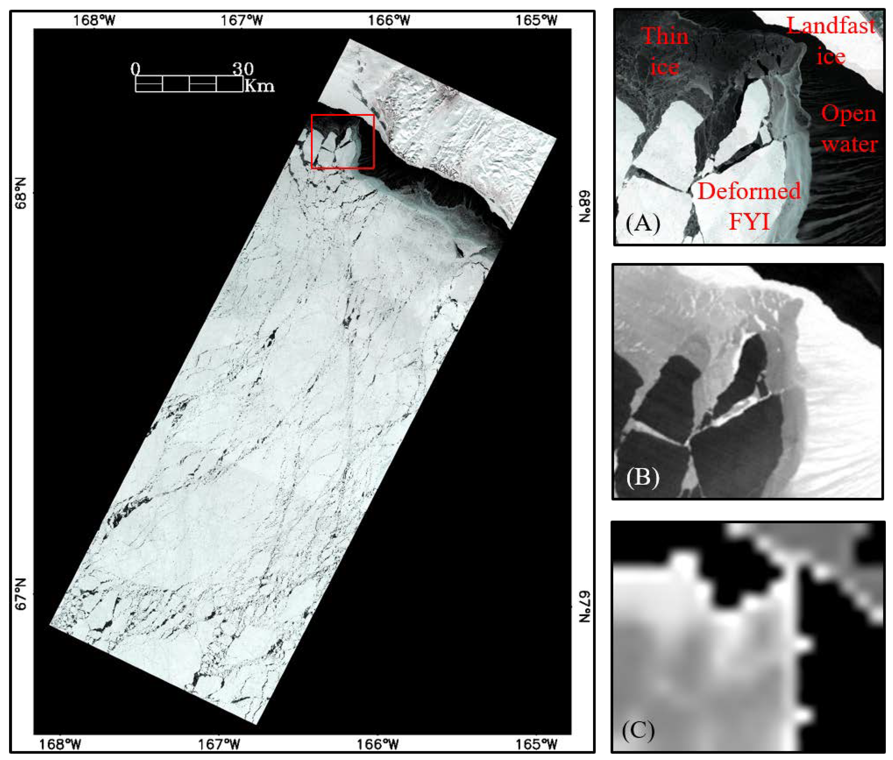
Figure 3.
Validation of MODIS IST using near-surface air temperature at the Alaskan tide stations (Prudhoe Bay, Nome, and Red Dog). There were matched within 30 min. The solid line is the 1:1 line. The dashed line is the best-fit line. The RMSE is the value with the bias removed.
Figure 3.
Validation of MODIS IST using near-surface air temperature at the Alaskan tide stations (Prudhoe Bay, Nome, and Red Dog). There were matched within 30 min. The solid line is the 1:1 line. The dashed line is the best-fit line. The RMSE is the value with the bias removed.
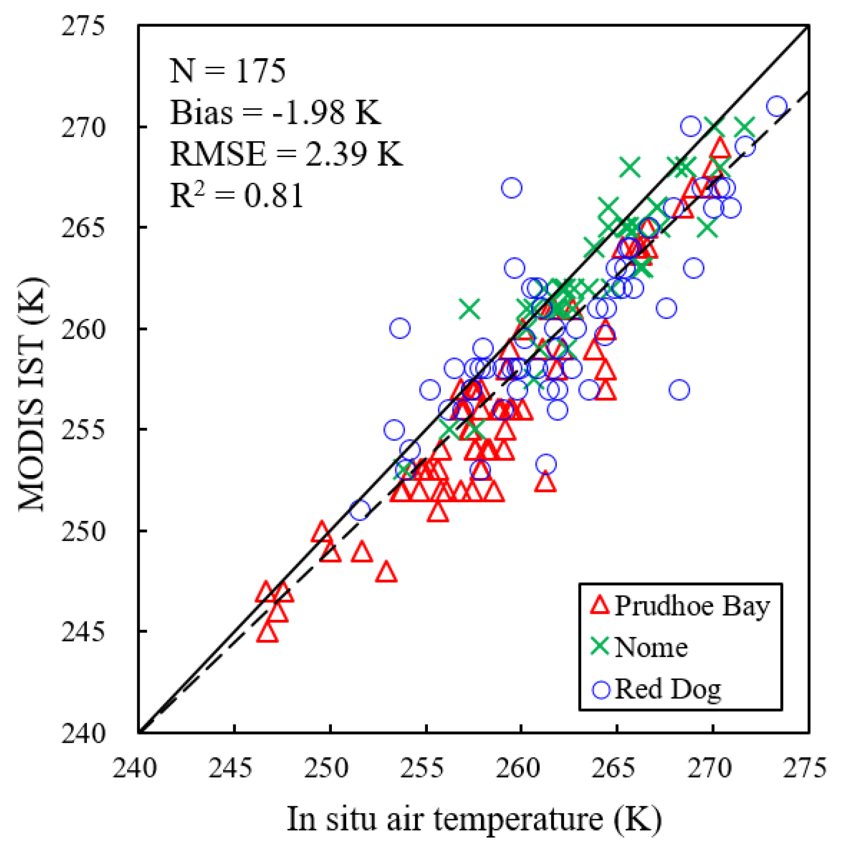
Figure 4.
Histogram of the SD of ASTER in a MODIS pixel for 17 ASTER scenes. The red line is the fitted Gaussian distribution, the solid black line is an average of the fitted Gaussian distribution, and the dashed black line is the average plus the SD. The blue line is the threshold for MODIS IST pixels representing homogeneous sea ice as true data.

Figure 5.
Scatter plots of MODIS IST versus ASTER brightness temperature for (A) band 10 through to (E) band 14 (n = 7938 × 121). The solid line is the 1:1 line. The dashed red line is the best-fit line.
Figure 5.
Scatter plots of MODIS IST versus ASTER brightness temperature for (A) band 10 through to (E) band 14 (n = 7938 × 121). The solid line is the 1:1 line. The dashed red line is the best-fit line.
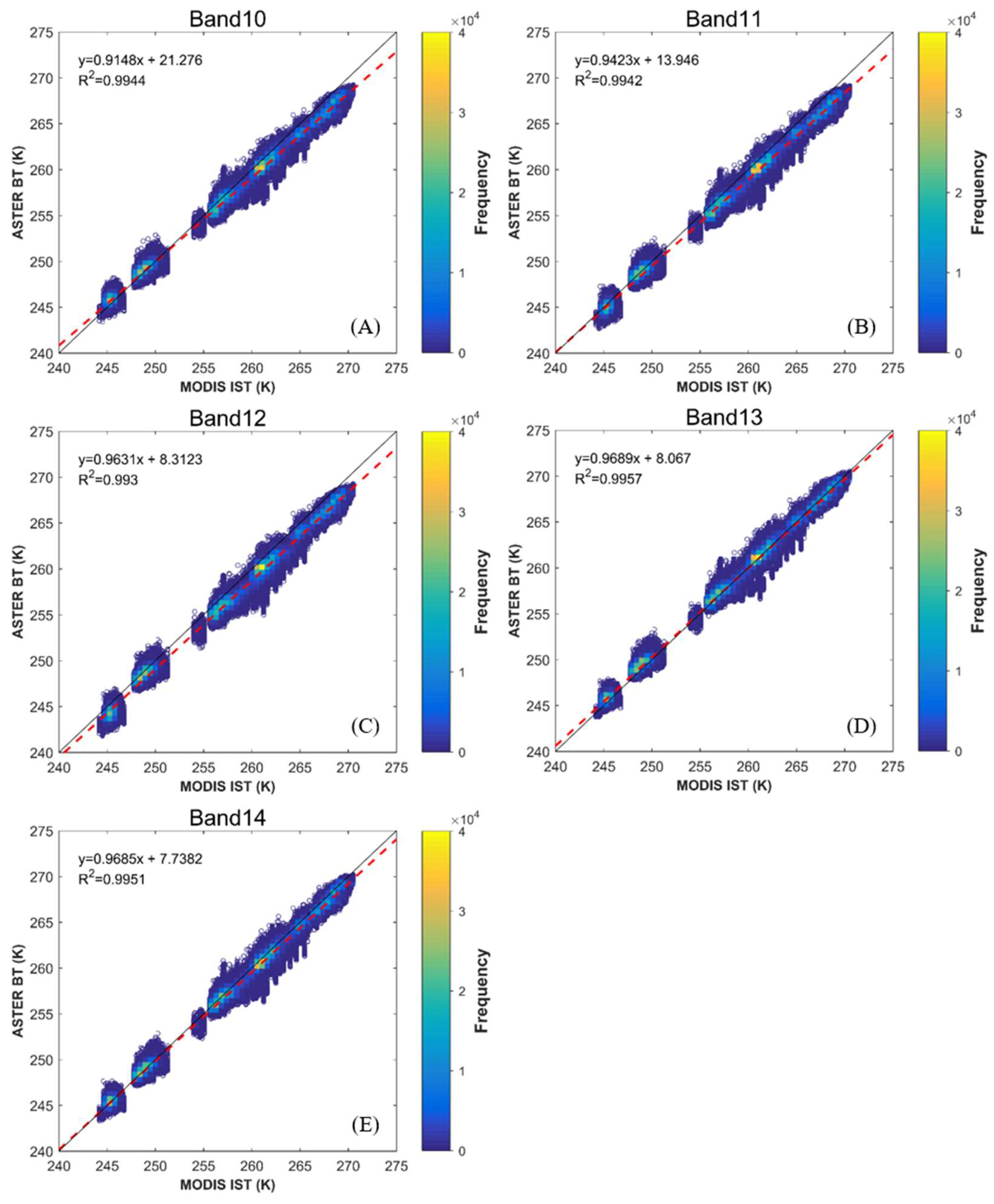
Figure 6.
Comparison between (A) MODIS IST versus ASTER IST using 17 ASTER scenes for algorithm development and (B) MODIS IST versus ASTER IST using seven ASTER scenes for algorithm validation. The solid line is the 1:1 line. The dashed red line is the best-fit line.
Figure 6.
Comparison between (A) MODIS IST versus ASTER IST using 17 ASTER scenes for algorithm development and (B) MODIS IST versus ASTER IST using seven ASTER scenes for algorithm validation. The solid line is the 1:1 line. The dashed red line is the best-fit line.
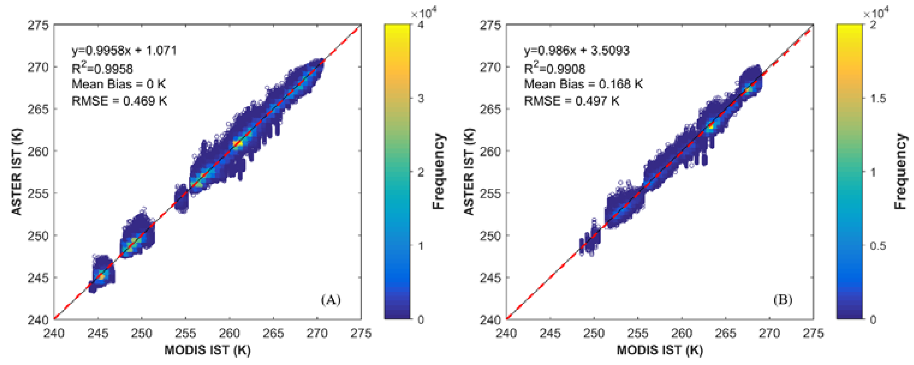
Figure 7.
(A) MODIS IST image and (B) ASTER IST image near Red Dog Dock. Thin ice or wetted ice types near the coast or in crevices had a higher temperature (yellow to red colors).
Figure 7.
(A) MODIS IST image and (B) ASTER IST image near Red Dog Dock. Thin ice or wetted ice types near the coast or in crevices had a higher temperature (yellow to red colors).


Table 1.
Comparison of thermal infrared region (TIR) band characteristics of sensors that can retrieve ice surface temperature (IST).
Table 1.
Comparison of thermal infrared region (TIR) band characteristics of sensors that can retrieve ice surface temperature (IST).
| Sensor | TIR Band No. | Spectral Range (μm) | Spatial Resolution |
|---|---|---|---|
| AVHRR | 4 | 10.30–11.30 | 1.09 km |
| 5 | 11.50–12.50 | ||
| MODIS | 31 | 10.78–11.28 | 1 km |
| 32 | 11.77–12.27 | ||
| VIIRS | M14 | 8.40–8.70 | 750 m |
| M15 | 10.263–11.263 | ||
| M16 | 11.538–12.488 | ||
| Landsat-8 | 10 | 10.30–11.30 | 100 m |
| 11 | 11.50–12.50 | ||
| ASTER | 10 | 8.125–8.475 | 90 m |
| 11 | 8.475–8.825 | ||
| 12 | 8.925–9.275 | ||
| 13 | 10.25–10.95 | ||
| 14 | 10.95–11.65 |
Table 2.
Information of ASTER scenes and MODIS IST for match-up.
| Type 1 | Region | ASTER Scene Date 2 | MODIS Pixel (Match-Up) 3 | MODIS IST Range (K) | Mean (SD) 4 (K) |
|---|---|---|---|---|---|
| D | Nome | 9 March 2001 | 78 (54) | 263.75–269.13 | 0.334 (0.13) |
| 26 April 2001 | 526 (526) | 267.8–270.52 | 0.168 (0.037) | ||
| 2 April 2004 | 475 (339) | 259.04–264.36 | 0.337 (0.131) | ||
| 14 April 2005 *** | 1144 (1069) | 260.02–270.06 | 0.239 (0.09) | ||
| Red Dog | 11 April 2002 | 667 (588) | 259.99–268.91 | 0.281 (0.11) | |
| 11 March 2003 *** | 1637 (1019) | 256.34–266.08 | 0.372 (0.147) | ||
| 20 April 2006 | 864 (541) | 252.98–259.99 | 0.366 (0.139) | ||
| 17 March 2007 | 864 (565) | 252.98–261.76 | 0.363 (0.134) | ||
| Prudhoe | 2 April 2001 ** | 1803 (1530) | 247.76–252.28 | 0.298 (0.112) | |
| 2 May 2002 ** | 1365 (870) | 260.22–264.24 | 0.341 (0.167) | ||
| 16 March 2008 | 1020 (837) | 244.05–246.96 | 0.329 (0.103) | ||
| Total | 17 | 11,404 (7938) | 244.05–270.52 | 0.319 (0.138) | |
| V | Nome | 17 March 2004 ** | 144 (77) | 257.08–261.04 | 0.402 (0.132) |
| 17 March 2007 ** | 877 (563) | 258.03–266.66 | 0.364 (0.162) | ||
| Red Dog | 26 April 2001 | 667 (603) | 266.69–268.91 | 0.27 (0.094) | |
| 24 March 2007 | 862 (596) | 247.56–261.76 | 0.358 (0.129) | ||
| Prudhoe | 3 May 2002 | 908 (614) | 264.23–265.46 | 0.338 (0.143) | |
| Total | 7 | 3458 (2453) | 247.56–268.91 | 0.339 (0.141) |
1 The types were divided into images for algorithm development (D) and for validation (V). 2, ** means a mosaic using two scenes, and *** means a mosaic using three scenes. 3 MODIS pixels had a SD of ASTER of less than 0.7 K and match-up pixels had a SD of ASTER of less than 0.4 K. 4 Mean of SD of ASTER in MODIS pixels with a SD of ASTER of less than 0.7 K.
Table 3.
Bias and RMSE between ASTER brightness temperature bands and MODIS IST.
| Range | ||||||
|---|---|---|---|---|---|---|
| Bias | >240 K | −0.705 | −0.955 | −1.197 | 0.031 | −0.402 |
| 240–260 K | 0.26 | −0.676 | −1.029 | 0.173 | −0.247 | |
| >260 K | −1.179 | −1.252 | −1.375 | −0.12 | −0.568 | |
| RMSE | >240 K | 1.06 | 1.167 | 1.361 | 0.515 | 0.678 |
| 240–260 K | 0.749 | 0.943 | 1.226 | 0.547 | 0.592 | |
| >260 K | 1.321 | 1.365 | 1.492 | 0.479 | 0.759 |
Table 4.
ASTER IST coefficients for Alaska coastal sea ice. Two-channel coefficients were used with Equation (4). Five-channel coefficients were used with Equation (5).
Table 4.
ASTER IST coefficients for Alaska coastal sea ice. Two-channel coefficients were used with Equation (4). Five-channel coefficients were used with Equation (5).
| Range | a | b | c | d | e | f | |
|---|---|---|---|---|---|---|---|
| 2 Ch | >240 K | −7.13193 | 1.02792 | −0.24093 | |||
| 240–260 K | −9.26874 | 1.03662 | −0.35169 | ||||
| >260 K | −5.95003 | 1.02318 | −0.11206 | ||||
| 5 Ch | >240 K | −9.733 | 0.149995 | 0.082399 | 0.028279 | 0.599756 | 0.178344 |
| 240–260 K | −12.9486 | 0.226197 | 0.073846 | −0.08225 | 0.552123 | 0.281406 | |
| >260 K | −8.60318 | 0.036583 | 0.134919 | 0.132995 | 0.697087 | 0.032862 |
Table 5.
Bias and RMSE for comparison of two-channel and five-channel algorithms for development and validation images.
Table 5.
Bias and RMSE for comparison of two-channel and five-channel algorithms for development and validation images.
| Type 1 | Coefficient | 2 Ch | 5 Ch | |
|---|---|---|---|---|
| D | All range | Bias | 0 | 0 |
| RMSE | 0.471 | 0.467 | ||
| Divided range | Bias | 0 | 0 | |
| RMSE | 0.469 | 0.462 | ||
| V | All range | Bias | 0.17 | 0.209 |
| RMSE | 0.497 | 0.507 | ||
| Divided range | Bias | 0.168 | 0.472 | |
| RMSE | 0.497 | 0.746 |
1 The types were divided into images for algorithm development (D) and for validation (V).
© 2018 by the authors. Licensee MDPI, Basel, Switzerland. This article is an open access article distributed under the terms and conditions of the Creative Commons Attribution (CC BY) license (http://creativecommons.org/licenses/by/4.0/).
Share and Cite
MDPI and ACS Style
Son, Y.-S.; Kim, H.-c.; Lee, S.J. ASTER-Derived High-Resolution Ice Surface Temperature for the Arctic Coast. Remote Sens. 2018, 10, 662. https://doi.org/10.3390/rs10050662
AMA Style
Son Y-S, Kim H-c, Lee SJ. ASTER-Derived High-Resolution Ice Surface Temperature for the Arctic Coast. Remote Sensing. 2018; 10(5):662. https://doi.org/10.3390/rs10050662
Chicago/Turabian StyleSon, Young-Sun, Hyun-cheol Kim, and Sung Jae Lee. 2018. "ASTER-Derived High-Resolution Ice Surface Temperature for the Arctic Coast" Remote Sensing 10, no. 5: 662. https://doi.org/10.3390/rs10050662
Note that from the first issue of 2016, this journal uses article numbers instead of page numbers. See further details here.