Automatic Discovery and Geotagging of Objects from Street View Imagery


ADAPT Centre, School of Computer Science and Statistics, Trinity College Dublin, Dublin 2, Ireland
*
Author to whom correspondence should be addressed.
Remote Sens. 2018, 10(5), 661; https://doi.org/10.3390/rs10050661
Submission received: 9 March 2018
/
Revised: 9 April 2018
/
Accepted: 18 April 2018
/
Published: 24 April 2018
(This article belongs to the Special Issue Multisensor Data Fusion in Remote Sensing)
Abstract
:Many applications, such as autonomous navigation, urban planning, and asset monitoring, rely on the availability of accurate information about objects and their geolocations. In this paper, we propose the automatic detection and computation of the coordinates of recurring stationary objects of interest using street view imagery. Our processing pipeline relies on two fully convolutional neural networks: the first segments objects in the images, while the second estimates their distance from the camera. To geolocate all the detected objects coherently we propose a novel custom Markov random field model to estimate the objects’ geolocation. The novelty of the resulting pipeline is the combined use of monocular depth estimation and triangulation to enable automatic mapping of complex scenes with the simultaneous presence of multiple, visually similar objects of interest. We validate experimentally the effectiveness of our approach on two object classes: traffic lights and telegraph poles. The experiments report high object recall rates and position precision of approximately 2 m, which is approaching the precision of single-frequency GPS receivers.
1. Introduction
The rapid development of computer vision and machine learning techniques in recent decades has excited the ever-growing interest in automatic analysis of huge image datasets accumulated by companies and individual users all worldwide. Image databases with Global Positioning System (GPS) information, such as Google Street View (GSV) and images posted on social networks like Twitter, are regularly updated, provide dense coverage of the majority of populated areas, and can be queried seamlessly using APIs. In particular, time-stamped geolocated panoramic images captured by cameras mounted on vehicles or carried by pedestrians are publicly accessible from GSV, Bing Streetside, Mapillary, OpenStreetCam, etc. This imaging modality is referred to as street view, street-level, or street-side imagery. Tens of billions of street view panoramas covering millions of kilometers of roads and depicting street scenes at regular intervals are available [1,2]. This incredible amount of image data allows one to address a multitude of mapping problems by exploring areas remotely, thus dramatically reducing the costs of in situ inventory, mapping, and monitoring campaigns.
Much research has been dedicated to leveraging street view imagery in combination with other data-sources such as remotely sensed imagery [3,4,5] or crowd-sourced information [6,7] to map particular types of objects or areas. Here we address the problem of automated discovery and geotagging of recurring objects using street view images as a sole source of input data. We consider any class of stationary objects sufficiently compact to have a single geotag that are typically located along the roads, such as street furniture (post boxes, various poles and street-lamps, traffic lights and signs, transport stops, benches, etc.), small facade elements (cameras, antennas, security alarm boxes, etc.), and other minor landmarks. Inventory and precise geolocation of such objects is a highly relevant task and, indeed, OpenStreetMap and Mapillary are currently encouraging their users to contribute such information to their databases manually. Nevertheless, the vast majority of these objects can be mapped automatically by efficiently exploring the street view imagery.
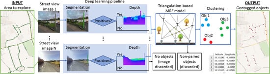
We propose a complete pipeline for the geotagging of recurring objects from street view imagery. The main components in the pipeline (see Figure 1) are two state-of-the-art fully convolutional neural networks (FCNN) for semantic segmentation and monocular depth estimation of street view imagery, and a novel geotagging model that estimates object locations by combining geographical camera location information from GPS and inertial measurement units (IMUs) with image analysis information. The information fusion is performed via a novel Markov random field (MRF) formulation that enables us to integrate depth information into geometric triangulation from object instances discovered in multiple street view images. Practically, the image processing scenario addressed in this work is tantamount to multi-sensor and multi-temporal information fusion since we discover and estimate locations of objects from images collected by optical cameras with different settings [8], of different imaging qualities [9], in different light and weather conditions, and on different dates.
In this work, we focus on geotagging recurring stationary objects that may be partially or completely occluded in some of the input images. We evaluate the performance of the proposed pipeline on two object classes: traffic lights and telegraph poles. Extensive experimental analysis confirms the accuracy of both object discovery and geotagging in comparison with a recent object mapping technique [10]. We also establish empirically that the accuracy of position estimation reported by our method approaches that achieved by single-frequency GPS receivers operating the Standard Positioning Service (SPS). Specifically, as reported in [11], the testing of GPS precision has demonstrated a m confidence interval for horizontal positioning achieved by SPS with a single-frequency receiver. One important contribution of this work is that our MRF-based geotagging procedure allows us to leverage monocular depth estimates to automatically resolve complex scenes containing multiple instances of identical objects, unlike previous works that rely on visual matching [10,12]. The proposed pipeline is modular which makes it possible to replace segmentation and depth modules with alternative techniques or pretrained solutions for particular object families. A demo video of our telegraph pole discovery and geotagging method can be viewed at https://youtu.be/X0tM_iSRJMw.
The paper is organized as follows: We first review some relevant state-of-the-art approaches in Section 2. Our complete geotagging pipeline is presented in Section 3 and then validated experimentally in Section 4. In Section 5, we discuss the inaccuracies associated with position estimation and in Section 6 conclude the study.
2. Related Work
In the last decade, a considerable effort has been directed towards the intelligent use of street view imagery in multiple areas such as mapping [4,6,13], image referencing [14], vegetation monitoring [15], navigation [3], and rendering and visualization [16,17]. Street view imagery has been combined with aerial imagery to achieve fine-grained road segmentation [3], land use classification [5], and tree detection/classification [4]. It is assumed that objects are discovered through both imaging modalities. Together with [12], these methods rely on a simplifying locally flat terrain model in order to estimate object locations from single street view images. LiDAR and 3D point cloud data have been used alongside street view imagery to perform land use classification [18], 3D segmentation [19], and change detection [20]. In [14,21], street view images are employed as references to geolocate query images by resorting to scene matching. The GSV imagery is employed in [16,17] in conjunction with social media, such as Twitter, to perform visualization and 3D rendering. Methods proposed in [22,23] target the inverse problem to the one addressed in this work: the street view camera position is inferred from access to geolocations of stationary objects. Much work has been done on monitoring and mapping from mobile LiDAR [24,25,26] and unmanned aerial vehicle (drones) [27,28]. These sensor modalities allow a more complete exploration of scenes and objects therein but are much less widely available than street view imagery.
Several methods have been developed to map particular types of objects from street-level imagery: manholes [12], telecom assets [10], road signs [29], and traffic lights [30,31]. These methods rely on position triangulation from individual camera views to geolocate the considered road furniture elements. All the approaches rely heavily on various geometrical and visual clues to perform matching whenever multiple objects are present in the same scene. As a consequence, whenever multiple identical objects are present simultaneously, these methods perform poorly. In particular, as pointed out in [10], visual matching performed via SIFT on street-level images with a strong view-point position change has limited performance in establishing reliable visual matches between small objects.
Image segmentation is one of the central tasks in object extraction. Many approaches have been proposed to address this problem: starting from elementary pattern analysis techniques, such as Hough transform and local gradients, through feature extraction-based tools that rely on cascades of weak classifiers [32], to more advanced machine learning methods such as random forests, support vector machines, and convolutional neural networks (CNNs) [33,34]. The latter have recently pushed the machine vision techniques to new heights by allowing automatic feature selection and unprecedented capacity to efficiently learn from considerably large volumes of data. FCNNs are a natural form of CNNs when addressing dense segmentation since they allow location information to be retained through the decision process by relying solely on convolutional layers [35]. Their output can be in the form of bounding boxes [36,37] or segmentation maps [35]. The latter are obtained via deconvolutions only or by resorting to conditional random fields [38].
Estimation of camera-to-object distances and, more generally, 3D scene analysis from RGB images can be addressed in several ways. The most explored are stereo-vision approaches [39] that estimate camera-to-object distances from multi-view stereo image disparity analysis or perform scene reconstruction via structure-from-motion methods [40]. These rely on various assumptions about camera positions and trajectory, and typically require a rich set of input RGB images and a certain form of knowledge about the analyzed scene. These methods rely heavily on feature extraction and matching. Monocular depth estimation is another way to address scene analysis and the relative positioning of objects therein. The central idea in this recent generation of techniques [41,42,43] is to recover depth information from monocular images based on the extensive scene interpretation capabilities of FCNNs by training them on RGB and depth or disparity images. These methods achieve consistent yet approximate results relying solely on the information available in the colour bands.
3. Object Discovery and Geotagging
Street view images are harvested by defining the area of interest and querying relevant APIs to download all the available imagery from camera positions located within. These are panoramic images supplied with the orientation information (bearing towards north). Images from multiple sources, providers, and/or databases can be combined, effectively increasing the volume of available data, as long as they are all provided with the camera’s position and orientation information.
Each image is processed independently allowing efficient parallelization of this most time-consuming step. All images reporting objects discovered by the FCNN segmentation module (see Section 3.1) are then processed by the monocular depth estimation module to produce estimates of camera-to-object distances (see Section 3.2) as presented in Figure 1. Image processing results are then fed into our MRF fusion module and finally clustered in order to obtain a coherent list of the detected object positions (see Section 3.3). The combination of fusion and clustering allows us to minimize the amount of duplicated objects that may appear due to sensor and segmentation noise.
Practically, we require the objects in the analyzed scenes to be sufficiently sparse to allow successful discrimination of distinct object instances by the segmentation pipeline. To this end, we enforce a mild assumption of object sparsity: objects of the same class are assumed to be located at least 1 m apart from each other. Whenever multiple objects are tightly clustered (i.e., with less than 1 m apart), they are likely to be discovered as a single object instance with a unique geotag.
3.1. Object Segmentation
One of the best-performing state-of-the-art semantic segmentation FCNN models [35] is adopted in our pipeline to perform object discovery. The subsampling part of this segmentation FCNN architecture is that of VGG-16 [34] with the fully connected layers converted to convolutional layers. These are followed by an upsampling (deconvolution) part that reverts from low-resolution segmentation to the original spatial resolution in several steps. The steps in this procedure allow for the combination of coarse segmentation maps with appearance information from shallower fine layers that have been generated by the subsampling part of FCNN. We employ the FCN-8s all-at-once model that reports the finest segmentation details by performing deconvolutions in the form of bilinear interpolations in three consecutive steps. The choice of pixel-level segmentation method as opposed to bounding box detectors [36,37] is due to the requirement to have pixel-level labels to merge individual monocular distances into a single object-to-camera estimate (see Section 3.2).
If we consider a single class of objects, we reshape all upsampling layers as well as the bottom convolution in the subsampling part to have two outputs—one for background and another for the objects of interest. In case of N classes of interest considered through a single FCNN segmentation module, the number of outputs in the upsampling part of the network should be set to .
We further add a second loss function (with the same weight) that penalizes only the false positives, thus effectively re-weighting the total loss to penalize false positives with a higher weight. This is due to our interpretation of the results where a small group of false positive pixels may result in a false positive object discovery, whereas missed pixels of a true object (false negatives) are less critical. Specifically, this second loss function is a modification of a standard Euclidean loss with the sum being calculated over false positives only, instead of summing all misclassified pixels. The final loss is a sum of softmax and the modified Euclidean, both with weights of .
3.2. Monocular Depth Estimation
Stereo-vision approaches are challenging when operating on street view imagery collected with an average acquisition step of 5–10 m. The main reason is that such sequences are typically characterized by substantial mismatch in scenes, which may be due to new objects on road sides, object scaling, moving vehicles, occlusions, panorama stitching artifacts, and, occasionally, distinct image acquisition dates. Furthermore, no a priori information is available on the geometry of the analyzed scenes. Thus, we chose to rely on approximate estimates reported by a recent FCNN depth estimation pipeline introduced in [42]. This architecture is composed of a fully convolutional version of ResNet-50 [33] followed by a cascade of residual up-projection blocks to obtain a dense depth map at the native image resolution. This pipeline is employed with no modifications and is fed only with the images where objects of interest are discovered by the segmentation module.
A unique depth estimate for each object is obtained by taking a -trimmed mean of the depths of its constituent pixels in a segmentation map. We apply trimming to gain robustness with respect to segmentation and depth estimation errors, in particular along the object borders.
3.3. Object Geotagging
Using the information extracted from images by the segmentation and monocular depth estimation modules, an estimate of the location of an object of interest can theoretically be obtained directly. This single view image strategy leads to inaccuracies and duplicates (see Section 3.3.1). Instead, in Section 3.3.2, we propose an alternative strategy based on intelligent information fusion from multiple images. Our approach is based on an MRF model with a custom grid defined by the available camera positions and detected objects (see Section 3.3.3).
3.3.1. Location from Single View
Consider a single street view image where objects of interest have been segmented. For each segmented region, a ray can be traced in 3D space from camera position towards the barycenter of the segmented region. A depth estimate for that region, obtained through averaging into a single object-level distance, allows the object’s location to be estimated. Specifically, from the segmentation map we extract the geo-orientation at which the object is located relative to the camera, shift the position by the estimated distance, and cast the coordinates into the target reference system (WGS-84).
There are two limitations associated with this strategy: Firstly, the depth estimates from the FCNN depth computation module have an approximative nature. Secondly, the list of all objects detected in the input images is largely redundant due to objects observed from multiple camera positions. Hence, each object spawns multiple detected object instances with substantially distinct locations estimated based on approximative depth estimates. An example of such estimates can be seen in Figure 2.
3.3.2. Location from Multiple Views
When an object is observed multiple times, the corresponding image segments need to be matched from different panoramas to group together observations of the same object-instances. Matching can be addressed in two ways: by relying on either general image features, such as SIFT, HOG, etc., or custom features extracted by the segmentation CNN. We have explored both ways, but neither provides satisfactory quality of matching due to a strong degree of similarity between the objects in the considered object-classes. Specifically, street-side objects tend to be identical in the same area, e.g., lines of poles along a road, traffic lights around the same road junction, manholes in the same area, etc. For this reason, the main source of dissimilarity detected through image matching is due to the background and occlusions in the object bounding boxes. The background composition, however, is subject to changes with the rotation of the viewing angle. Note also that the considered objects are in the proximity of roads, hence a small change in angle may result in strong dissimilarity of image background and thus upset object matching. The available imagery is often provided at too low a resolution to allow reliable visual assessment of small and medium objects, which is necessary to perform the matching reliably.
Similarly to [10], we have observed that visual matching is not sufficient to reliably identify individual object instances in scenes with multiple similar or identical objects of interest. In this work, we choose not to resort to preset object sizes or shapes that may assist in matching and depth estimation of particular object families. This choice allows us to preserve the generality of the designed methodology. Instead, we explore alternatives to achieve object-instance pairing.
To perform position estimation, we rely on a mixed approach based on triangulation. For illustration purposes, in Figure 2, we present an example of a simple stationary scene observed using three cameras or equivalently, using the same camera at three successive locations. Three objects of interest (traffic lights) are present in the scene. Object1 is detected in all images, Object2 is missed in images collected by Camera1 (segmentation false negative), and Object3 is occluded from Camera2. A false positive is picked up in the Camera1 image. Figure 2 demonstrates the complexity of accurately triangulating three objects in the space of 13 intersections. Spurious intersections do not correspond to real objects (yellow). A single object may correspond to multiple pairwise ray intersections (see Object1) due to camera position noise and inaccuracies in object segmentation. Note that the candidate intersections are located such that clustering or grouping them without intelligent interpretation leads to completely wrong sets of object geolocations.
3.3.3. MRF Formulation with Irregular Grid
To address the problem of automatic mapping in multi-object scenes, we propose an MRF-based optimization approach. This flexible technique allows us to incorporate the approximate knowledge about the camera-to-object distances into the decision process. Furthermore, it can be seen as a generalization to the previously proposed methods [10,12] as it allows the integration of geometry/visual-based matching as additional energy terms. The designed MRF model operates on an irregular grid that consists of all of the intersections of view rays generated by object instances detected at the object segmentation step. Specifically, we consider each detected object as a ray from camera position in the direction of the baricentre of the corresponding segment of pixels. MRF cliques include all intersections found on the two view rays generating an intersection. These cliques reflect the local interactions, and the neighbourhood sizes vary depending on the site. We employ custom MRF energy terms to incorporate all available information for object localization: monocular depth estimates and geometric rules governing the space of intersections.
MRF setup. We consider the space of all pairwise intersections of view-rays from camera locations (see Figure 2). Any location is generated by the intersection of two rays and from the camera view pair. The binary label is associated with x to indicate the presence (, referred to as positive intersection depicted as blue dots in Figure 2) or absence (, empty intersection, yellow in Figure 2) of the object of interest at the corresponding intersection (see side panel in Figure 2). The space of all intersections’ labels is then a binary MRF [44], which is formally defined as follows:
- To each site x we associate two Euclidean distances and from cameras: , where are the locations of two cameras from which intersection x is observed along the rays and , respectively. Any intersection x is considered in , only if . In Figure 2, the red intersection in the upper part of the scene is rejected as too distant from Camera3.
- The neighbourhood of node x is defined as the set of all other locations in on the rays and that generate it. We define the MRF such that the state of each intersection depends only on its neighbours on the rays. Note that the number of neighbours (i.e., neighbourhood size) for each node x in in our MRF varies depending on x.
- Any ray can have at most one positive intersection with rays from any particular camera, but several positive intersections with rays generated from different cameras are allowed, e.g., multiple intersections for Object1 in Figure 2.
MRF energy. The full MRF configuration is defined as the set of all pairs (location, label): . As established by the Hammersley–Clifford theorem [44] probabilities of the MRF states are governed by Gibbs distribution:
where is the vector of model parameters, is the energy function corresponding to the configuration , and is the normalising coefficient. For each site x with state z, the associated MRF energy is composed of the following terms:
- A unary energy term enforces consistency with the depth estimation. Specifically, the deep learning pipeline for depth estimation provides estimates and of distances between camera positions and the detected object at location x. We formulate the term as a penalty for mismatch between triangulated distances and depth estimates:
- A pairwise energy term is introduced to penalize (i) multiple objects of interest occluding each other and (ii) excessive spread, in case an object is characterized as several intersections. In other words, we tolerate several positive intersections on the same ray only when they are in close proximity. This may occur in a multi-view scenario due to segmentation inaccuracies and noise in camera geotags. For example, in Figure 2, Object1 is detected as a triangle of positive intersections (blue dots)—two on each of the three rays.Two distant positive intersections on the same ray correspond to a scenario when an object closer to the camera occludes the second, more distant object. Since we consider compact slim objects, we can assume that this type of occlusion is unlikely.This term depends on the current state z and those of its neighbours . It penalizes proportionally to the distance to any other positive intersections on rays and :
- A final energy term penalizes rays that have no positive intersections: false positives or objects discovered from a single camera position (see Figure 2). This can be written aswhere k indexes all other intersections along the two rays defining the current intersection.It is also possible to register rays with no positive intersections as detected objects by applying the depth estimates directly to calculate the geotags. The corresponding positions are of lower spatial accuracy but allow an increase in the recall of object detection. In this study, we discard such rays to increase object detection precision by improving robustness to segmentation false positives.
The full energy of configuration in is then defined as the sum of energy contributions over all sites in :
with parameter vector subject to , .
The optimal configuration is characterized by the global minimum of the energy . The terms and penalize too many objects to be found by increasing the total energy (for any positive intersection with both and ), whereas penalizes when too few objects are found ( for any ray with no positive intersections). The MRF formulation can also explicitly accommodate object location pattern assumptions through additional higher-order penalty terms.
MRF optimization. We perform energy minimization with an iterative conditional modes algorithm [44] starting from an empty configuration: . This (local) optimization is run according to a random node-revisiting schedule until a local minimum is reached and no further changes are accepted. Experimentally, we have observed stable performance of the optimizer over multiple reruns. In case of particularly complex scenes with tens of objects in close vicinity, more comprehensive exploration of the energy landscape may be required, which can be achieved via simulated annealing (see [44]). Optimization with non-stochastic techniques such as graph cuts poses difficulties due to a high-order energy term and an irregular MRF grid.
Clustering. The final object location is obtained using clustering to merge positive intersections concentrated in the same area that are likely to describe the same object. Indeed, this is required since we consider the space of all pairwise intersections, whereas some objects are observed from three or more camera positions and result in multiple detected object instances due to noise on input data (i.e., in GPS, IMUs, and image data). For example, in Figure 2, Object1 is identified as three distinct positive intersections tightly scattered around the object. In this work we employ hierarchical clustering with a maximum intra-cluster distance of 1 m which corresponds to our object sparsity assumption. Coordinates of positive intersections in the same cluster are averaged to obtain the final object’s geotag.
Operationally, clustering is also useful for parallelising the geotagging step by splitting the analyzed large area in several smaller connective parts, with an overlap of a −25 m buffer zone that belongs to areas on both sides of any border. This strategy allows us to retain all rays for triangulation, while clustering resolves the object redundancies when merging the parts into a single object map.
4. Experimental Results
We test our pipeline on GSV imagery for detection of two object types: traffic lights and telegraph poles. Both kinds of objects are compact enough to be attributed a single geotag and are predominantly visible from roads. Traffic lights are visible by design and telegraph poles are also typically erected in close vicinity of the road network. Both of the object classes cannot be reliably detected in nadir/oblique airborne/satellite imagery due to their compact sizes and minimal footprint. Hence, street view is the appropriate imaging modality to perform their discovery and geotagging.
In order to evaluate the accuracy of the estimated object coordinates, we deploy our detector in several areas covered by GSV imagery. To extract the latter, we first create a dense grid of points along road-centers with a 3 m step and then query the corresponding Google API to retrieve the closest available GSV panoramas in 4 parts, each with a 90 field of view at pixels resolution. Note that GSV imagery often demonstrates strong stitching and blurring artifacts, in particular, in the top and bottom parts of the images (see examples in Section 4.2).
For the segmentation FCNN we use a Caffe implementation and perform training on a single NVIDIA Titan Xp GPU using stochastic gradient descent with a fixed learning rate of and momentum , with batches of two images. This choice is in line with recommendations in [35] and has empirically demonstrated best performances. We augment the data by performing random horizontal flipping, rotations , and small enhancements in the input image’s brightness, sharpness, and colour. The former two are used to augment the training dataset and the latter are employed to simulate different imaging conditions and calibration camera settings, since Google does not disclose these for their imaging systems. The imbalance between classes-object and background—in the datasets is handled well by the FCNN, provided we maintain a fraction of object-containing images in the training set above at all times. The inference speed is at 10 fps. To further increase the robustness to false positives, we only consider segments containing at least 100 pixels. The monocular depth estimation module [42] is used in the authors’ implementation in MatConvNet with no modifications. The energy weights in Equation (5) are set to and . Both segmentation FCNN loss functions have the same weight.
4.1. Geolocation of Traffic Lights
Training. The image segmentation pipeline for traffic lights is trained on data from two publicly available datasets with pixel-level annotations: Mapillary Vistas [45] and Cityscapes [46]. We crop/resize the images to match the standard GSV image size of . This provides us with approximately 18.5 K training images containing large traffic lights (at least pixels each instance). We start with a PASCAL VOC-pretrained model and carry on training with a learning rate of for another 200 epochs.
Dataset. To evaluate the geotagging performance, we consider a 0.8 km stretch of Regent street in London, UK, covered by 87 GSV panoramas (collected in January–June 2017) (see Figure 3). This dense urban area has five clusters of traffic lights, totalling 50 individual objects. To avoid ambiguity in the count, we assume that traffic lights attached to a single pole are counted as a single object. Note that we do not have access to precise coordinates of traffic lights and The ground truth positions are collected based on a human interpretation of GSV images.
We consider objects to be recovered accurately if they are located within 2 m from the ground truth position. This choice is in line with the official reports on the accuracy of GPS measurements that establish a m confidence interval for horizontal error for single-frequency GPS receivers operating according to the SPS [11].
Object detection. The test pixel-level precision plateaus at and recall at . If over of an object’s pixels are labelled correctly, we consider such object instances to be recovered accurately. In the vicinity of a camera (within 25 m from the camera’s position), the instance-level precision is and the recall is in the test set. In this experiment, the introduction of the second FCNN loss function improved the instance-level precision by and decreased the recall by . In general, instance-level recall is a more important characteristic for the geotagging of objects, whereas a lower precision (false positives) is partially compensated at the later stage by the employed tagging procedure, which requires objects to be observed multiple times. In this study, we adopt a conservative strategy of ignoring objects located farther than 25 m from camera positions due to the pronounced performance drop in image processing reliability for distant objects: a substantial decrease in the recall rate in semantic segmentation and high variance in depth estimation. Note that farther objects may be discovered through semantic segmentation but are rejected by the geotagging procedure described in Section 3.3 through the maximal distance restriction.
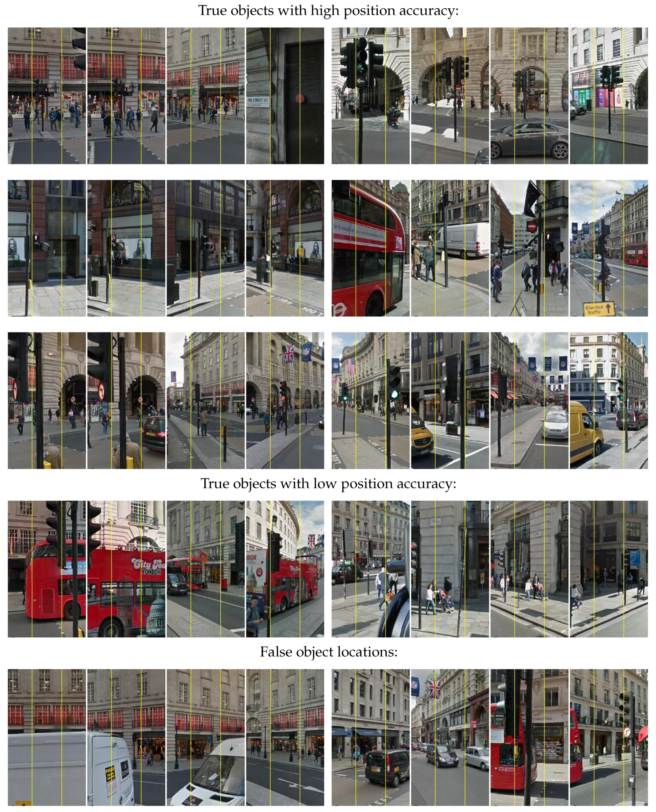
In Figure 4, we show examples of traffic light segmentation in busy urban scenes. The performance is overall very good with minor issues of occasional small false positives and of some traffic lights facing away from the camera (see images in central and right columns). Neither of the two poses particular problems for geotagging since the processing is done on a series of images, which allows us to observe most traffic lights both from front and rear and discard false positives due to their inconsistent and/or non-stationary nature. As far as the pixel-level performance is concerned a high precision rate is not necessary since we require pixel-level labels solely to access the relevant depth estimates obtained through the depth evaluation pipeline.
Geotagging. Segmentation reports 179 single-view traffic lights instances with 70 objects in 51 clusters after geotagging (to compare with 50 ground truth objects). The object discovery results are summarized in Table 1 (top row). The obtained object recovery precision and recall are both above and consistently outperform results of (maximum) reported for telecom assets recognition in [10]. Of the four false positives, two correspond to actual objects that are approximatively 3 m away from their ground truth locations. Six single-view instances were not matched: four segmentation were false positives, while two objects were only detected from one view.
Finally, in Figure 5, we demonstrate the detection accuracy qualitatively by viewing some of the estimated objects’ positions from multiple camera locations. To this end, we employ more recent imagery than that used for object detection: we select panoramas collected after July 2017. For each estimated traffic light, we randomly select four GSV camera positions in 20 m vicinity and present crops from panoramas oriented towards the estimated object’s position. In some of the views, traffic lights are occluded from view by walls and moving vehicles. The visual analysis confirms the high accuracy of geotagging with 44 out of 50 objects correctly detected within 2 m of their ground truth position. False object locations originate from either segmentation faults (road sign in the left multi-view panel, bottom row) or the erroneous selection of viewing rays intersections, which results in observation of traffic lights from some camera positions and no objects of interest from others (right panel, bottom row).
4.2. Geolocation of Telegraph Poles
We consider here a particular class of telegraph poles that are in use in the Republic of Ireland. The corresponding network is very large with over a million of poles spread throughout the country. All of these poles are made of wood and visually have a natural ‘wooden’ texture (no artificial colouring due to paint). Other more subtle distinctive visual features of telegraph poles include steps for climbing, particular types of insulation, and mounted objects. None of these are necessarily present (or visible) on any particular telegraph pole. Vegetation provides another complication for pole detection: these are often overgrown by ivy or closely surrounded by trees. Overall, the main challenge in detection of such poles is their strong visual similarity to all other tall poles, in particular, lampposts and electricity poles.
Training. Segmentation of the telegraph poles relies on a custom training dataset. Indeed, even though multiple existing datasets incorporate class ‘poles’, none provides sufficient distinction between different types of poles: lampposts, poles supporting traffic lights or road signs, bollards (sidewalk poles), and utility poles (electricity, telegraph). To train an FCNN classifier for this custom object type, we employ a multi-step training procedure:
- Image filtering. We start with a small dataset of 1 K manually chosen GSV images containing telegraph poles. We define a simple filtering procedure to automatically identify the location of poles in the images by a combination of elementary image processing techniques: Sobel vertical edge extraction, Radon maxima extraction, and colour thresholding. We also remove ‘sky’ pixels from the background as identified by the FCNN [35]. This allows us to extract rough bounding boxes around strong vertical features like poles.
- Cascade classifier. We then train a cascade classifier [32] on 1 K bounding boxes produced at the previous step. Experimentally, the recall achieved on poles is about with a precision of . We employ this classifier to put together a larger telegraph pole dataset that can be used to train segmentation FCNN. To this end, we use a training database of telegraph poles’ positions made available to us for this study. Specifically, we extract GSV images closest in locations to the poles in the database whenever GSV imagery is available within a 25 m radius. Due to the inherent position inaccuracy in both pole and GSV positions and frequent occlusions, we cannot expect to observe poles at the view angle calculated purely based on the available coordinates. Instead, we deploy the cascade classifier trained above to identify poles inside panoramas. Since many of the images depict geometry-rich scenes and since some telegraph poles may be occluded by objects or vegetation, in about of cases, we end up with non-telegraph poles as well as occasional strong vertical features, such as tree trunks, roof drain pipes, and antennas. Thus, we prepare 130 K panoramic images with bounding boxes.We next identify the outlines of poles inside the bounding boxes by relying on the image processing procedures proposed in the first step. This allows us to provide coarse boundaries of telegraph poles for the training of an FCNN. The resulting training dataset consists of an estimated of telegraph poles, about of other types of poles, and about of non-pole objects.
- FCNN training: all poles. We then train our FCNN to detect all tall poles—utilities and lampposts—by combining public datasets Mapillary Vistas [45] and Cityscapes [46] with the dataset prepared in the previous step. The inclusion of public datasets allows us to dramatically increase robustness with respect to background objects, which are largely underrepresented in the dataset prepared above with outlines of poles.The public datasets provide around 20 K images, so the merged dataset contains 150 K images: 130 K training and 20 K validation. This first step of training is run for 100 epochs at a learning rate of to achieve satisfactory discriminative power between poles and non-poles.
- FCNN fine-tuning: telegraph poles. The final second step of FCNN training is performed by fine-tuning the network on our custom pixel-level annotated set of 500 telegraph pole images. To further boost the discriminative power of the FCNN, we add 15 K GSV scenes collected in areas with no telegraph poles but in the presence of lampposts and electricity poles. The fine-tuning phase is run for another 200 epochs at a learning rate of .
To explore fully the performance and accuracy of the proposed pipeline, we present two case studies for the telegraph poles: small-scale Study A and large-scale Study B. The former investigates the capacity to detect and geolocate objects in a complex, geometry-rich, urban environment. The latter addresses the larger-scale performance of the proposed methodology in rural areas.
4.2.1. Study A: Small-Scale, Urban
Dataset. We perform experimental analysis in the Rathmines area of Dublin, Ireland (see Figure 6). The area under study has approximately 8 km of roads covered by 945 GSV panoramas. Seventy-seven telegraph poles are visible through the GSV imagery. The ground truth has been manually collected with a single-frequency GPS device: each pair of coordinates has been recorded three times on three different days and averaged to produce a single reference geotag for each object.
Object detection. Sample pole segmentation maps are presented in Figure 7. The final FCNN reports a pixel-level recall of and a precision . As above, we consider relevant only the objects within 25 m of the camera. This ensures accurate distinction from other tall poles since the decisive subtle differences are not visible at greater distances. The object-level test recall is and the precision is . The image segmentation module discovered 273 single-view instances.
Geotagging. The geotagging results are summarized in Table 1 (middle row). Out of the three false positives: two are wrong objects, and one is a telegraph pole 3 m away from its true location. To compare the accuracy of mapping with [10], we estimated the relative distance precision (calculated distance/ground truth object-to-camera distance × ). With this metric, we achieve a average and an standard deviation, which is an improvement upon the average reported in [10].
Additionally, we evaluate the absolute accuracy of positioning of objects: Table 2 reports the empirical statistics of object position estimation error (absolute value of the distance between the reference and triangulated positions): mean, median, variance, empirical confidence interval. Notably, the obtained interval of m is approaching the m confidence interval for single-frequency GPS receivers with SPS [11]. Practically, this implies that the accuracy of automatic mapping achieved by our method is equivalent to that of a human operator manually performing object mapping with a commercial-level GPS-enabled device.
In Table 2, we report the results of geotagging based on depth estimation from 89 monocular views, without resorting to triangulation. We observe a substantial improvement over the position estimation accuracy obtained with our triangulation procedure. In both cases—MRF triangulation and depth FCNN—the geotags rely entirely on the accuracy of the input camera coordinates provided with GSV imagery. Any outliers in camera geolocations result directly in object geotag errors.
4.2.2. Study B: Large-Scale, Rural
To validate the performance on a large-scale problem, we deployed the detector on a cluster of 120 km of public roads in County Mayo, Ireland, captured by GSV panoramas. This area has extensive networks of telegraph and electrical poles. Electricity poles detected by the geotagging pipeline are considered false positives even if there is no visual evidence to allow telegraph vs. electricity pole discrimination. Severe occlusions by vegetation are present in the area as well.
Dataset. We had access to the inventory of ground truth locations for 2696 telegraph poles in that area as recorded by the Irish telecom company Eir. The position accuracy of ground truth records is heterogeneous, as it has been recorded over a long period of time using different methods and by different operators. We therefore utilize this ground truth solely to validate the recall and precision of the pipeline but not to validate the accuracy of the coordinates computed with our pipeline. A detected pole is considered true positive if it is within 3 m of a recorded object. This choice of distance is due to limited quality of position records available in the area.
Geotagging. The validation results are summarized in Table 1 (bottom row). We observe similar performance as reported above. A slightly lower recall occurs because the ground truth records are collected manually and include many road-side poles completely occluded from view by vegetation. Higher precision is achieved due to the relative complexity of the urban environment compared to the mostly rural imagery depicting less challenging geometries processed in this experiment.
In this experiment, an average of 1.56 objects is typically observed per image reporting any detections. This occurs because telegraph poles are typically parts of longer pole-lines and several identical poles are often visible from the same camera position. This highlights the necessity for non-standard triangulation such as our MRF-based technique to enable object mapping. In the considered road cluster around of the pole-containing scenes cannot be mapped using methods similar to those proposed in [10,12,29] due to the presence of multiple visually identical telegraph poles, which renders visual matching-based triangulation inefficient.
5. Discussion
The empirical accuracy of the geotagging is characterized by a 2 m 95% confidence interval, which approaches to that obtained with SPS GPS on a single-frequency GPS receiver [11]. The three sources of the inaccuracy contributing to this value of the empirical confidence interval are (i) MRF triangulation errors, (ii) noisy object segmentation, and (iii) GPS inaccuracy of camera positions. The first can be improved by incorporating additional information about objects positions, e.g., detection from airborne/satellite imagery, matches from LiDAR/3D point cloud data, GIS information from existing maps, and a priori information about relative positioning of the objects of interest. A helpful simplifying assumption is a known preset width of objects that allows to refine the quality of depth estimates. Any such information can alleviate the object sparsity assumption adopted in this work. The proposed object position estimation approach is MRF-based and thus offers a convenient way of integrating any new information about the objects into the decision process by adding dedicated energy terms. The inaccuracy originating from image segmentation faults can be reduced by adopting the cutting-edge best performing detection pipelines developed for particular class of objects. Nevertheless, there is a limit to such improvements since objects may be aligned such that multiple object instances are merged in images or their positions are invisible to camera due to occlusions from other stationary or moving objects. The third source of inaccuracies may be addressed by the suppression of camera position noise or outliers.
In this work, we focus on the estimation of objects’ horizontal positions. The triangulation procedure does not allow one to automatically address the problem of vertical position estimation (elevation above the ground level). This may be performed by relying on the following simplifications: locally flat terrain model and preset vertical sizes of objects. Furthermore, these simplifying assumptions may also improve the quality of horizontal position estimation similarly to a fixed width assumption. Note that, in the proposed position estimation approach, we do not rely on a flat terrain assumption: as long as there are no optical distortions in the images, triangulation allows one to recover precise horizontal positions regardless of relative vertical elevation of the objects.
The empirical object discovery accuracies summarized in Table 1 report 2–4% of false positives and approximately of false negatives in telegraph pole detection (both studies). This conservative behaviour is promoted by the loss function of segmentation pipeline, which penalizes false positives stronger than false negatives. This effect is further increased by clustering, which reduces the number of redundant detections (false positives) due to multiple pairwise view-ray intersections for objects discovered in three or more images. This conservative detection bias can be inverted if required by the considered application by reducing the weight of the second loss term in segmentation.
One of the directions for future work would be the design of a unified FCNN architecture to perform segmentation and monocular depth estimation. In the absence of a priori depth data, such unified architecture can be trained as the second stage on the results of the object discovery procedure presented here. This may allow for partial or complete relaxation of the sparsity assumptions by providing improved quality input to the MRF-based geotagging pipeline.
6. Conclusions
We have proposed an automatic technique for detection and geotagging recurring stationary objects from street view imagery. Our approach is not restricted to any specific type of object as long as detected objects are compact enough to be described by a single geotag. The proposed solution relies on two existing deep learning pipelines: one fine-tuned for the considered segmentation scenario and the other employed for monocular depth estimation without modifications. A novel triangulation-based MRF has been formulated to estimate object geolocations that allows us to handle automatically any multi-object scenes. The triangulation helps to avoid duplicates and simultaneously reduce the number of false positives. This geotagging module is independent and can be combined with any other segmentation and/or depth estimation pipelines fine-tuned for specific object classes. The experimental analysis has demonstrated high object recall rates of 92–95% on complex scenes with two considered types of objects: traffic lights and telegraph poles, in urban and rural scenes. The position estimation accuracy is characterized by approximately 2 m empirical confidence interval. The Python implementation of the geotagging pipeline as well as the employed traffic lights dataset are available at github.com/vlkryl/streetview_objectmapping.
Author Contributions
Vladimir A. Krylov and Eamonn Kenny prepared the data and performed the experiments; Vladimir A. Krylov, Eamonn Kenny, and Rozenn Dahyot conceived the experiments; Vladimir A. Krylov and Rozenn Dahyot wrote the paper.
Acknowledgments
This research was supported by eir—the principal provider of fixed-line and mobile telecommunications services in Ireland—who are actively investing in research on machine learning and image processing for the purposes of network planning and maintenance. This research was also supported by the ADAPT Centre for Digital Content Technology, which is funded under the Science Foundation Ireland Research Centres Programme (Grant 13/RC/2106) and is co-funded under the European Regional Development Fund. We gratefully acknowledge the support of NVIDIA Corporation with the donation of the Titan Xp GPU used for this research.
Conflicts of Interest
The authors declare no conflict of interest.
References
- BBC News. Google’s Street View Cameras Get Quality Boost. 6 September 2017. Available online: http://www.bbc.com/news/technology-41082920 (accessed on 20 April 2018).
- Mapillary: Celebrating 200 Million Images. 5 October 2017. Available online: https://blog.mapillary.com/update/2017/10/05/200-million-images.html (accessed on 20 April 2018).
- Mattyus, G.; Wang, S.; Fidler, S.; Urtasun, R. HD maps: Fine-grained road segmentation by parsing ground and aerial images. In Proceedings of the 2016 IEEE Conference on Computer Vision and Pattern Recognition (CVPR), Las Vegas, NV, USA, 26 June–1 July 2016; pp. 3611–3619. [Google Scholar]
- Wegner, J.D.; Branson, S.; Hall, D.; Schindler, K.; Perona, P. Cataloging public objects using aerial and street-level images-urban trees. In Proceedings of the 2016 IEEE Conference on Computer Vision and Pattern Recognition, Las Vegas, NV, USA, 26 June–1 July 2016; pp. 6014–6023. [Google Scholar]
- Workman, S.; Zhai, M.; Crandall, D.J.; Jacobs, N. A unified model for near and remote sensing. In Proceedings of the 2017 IEEE Conference on Computer Vision and Pattern Recognition (CVPR), Honolulu, HI, USA, 21–26 July 2017; Volume 7. [Google Scholar]
- Hara, K.; Azenkot, S.; Campbell, M.; Bennett, C.L.; Le, V.; Pannella, S.; Moore, R.; Minckler, K.; Ng, R.H.; Froehlich, J.E. Improving public transit accessibility for blind riders by crowdsourcing bus stop landmark locations with Google Street View: An extended analysis. ACM Trans. Access. Comput. 2015, 6, 5. [Google Scholar] [CrossRef]
- Wang, X.; Zheng, X.; Zhang, Q.; Wang, T.; Shen, D. Crowdsourcing in ITS: The state of the work and the networking. IEEE Trans. Intell. Transp. Syst. 2016, 17, 1596–1605. [Google Scholar] [CrossRef]
- Wired. Google’s New Street View Cameras will Help Algorithms Index the Real World. 9 May 2017. Available online: https://www.wired.com/story/googles-new-street-view-cameras-will-help-algorithms-index-the-real-world/ (accessed on 20 April 2018).
- Seamless Google Street View Panoramas. 9 November 2017. Available online: https://research.googleblog.com/2017/11/seamless-google-street-view-panoramas.html (accessed on 20 April 2018).
- Hebbalaguppe, R.; Garg, G.; Hassan, E.; Ghosh, H.; Verma, A. Telecom Inventory management via object recognition and localisation on Google Street View Images. In Proceedings of the 2017 IEEE Winter Conference on Applications of Computer Vision (WACV), Santa Rosa, CA, USA, 24–31 March 2017; pp. 725–733. [Google Scholar]
- Federal Aviation Administration. Global Positioning System (GPS) Standard Positioning Service (SPS) Performance Analysis Report #100; Technical Report; Federal Aviation Administration: Washington, DC, USA, January 2018.
- Timofte, R.; Van Gool, L. Multi-view manhole detection, recognition, and 3D localisation. In Proceedings of the 2011 IEEE International Conference on Computer Vision Workshops (ICCV Workshops), Barcelona, Spain, 6–13 November 2011; pp. 188–195. [Google Scholar]
- Lefèvre, S.; Tuia, D.; Wegner, J.D.; Produit, T.; Nassaar, A.S. Toward Seamless Multiview Scene Analysis From Satellite to Street Level. Proc. IEEE 2017, 105, 1884–1899. [Google Scholar] [CrossRef]
- Hays, J.; Efros, A.A. IM2GPS: Estimating geographic information from a single image. In Proceedings of the IEEE Conference on Computer Vision and Pattern Recognition (CVPR), Anchorage, Alaska, 23–28 June 2008; pp. 1–8. [Google Scholar]
- Li, X.; Zhang, C.; Li, W.; Ricard, R.; Meng, Q.; Zhang, W. Assessing street-level urban greenery using Google Street View and a modified green view index. Urban For. Urban Green. 2015, 14, 675–685. [Google Scholar] [CrossRef]
- Bulbul, A.; Dahyot, R. Social media based 3D visual popularity. Comput. Graph. 2017, 63, 28–36. [Google Scholar] [CrossRef]
- Du, R.; Varshney, A. Social Street View: Blending Immersive Street Views with Geo-tagged Social Media. In Proceedings of the International Conference on Web3D Technology, Anaheim, CA, USA, 22–24 July 2016; pp. 77–85. [Google Scholar]
- Zhang, W.; Li, W.; Zhang, C.; Hanink, D.M.; Li, X.; Wang, W. Parcel-based urban land use classification in megacity using airborne LiDAR, high resolution orthoimagery, and Google Street View. Comput. Environ. Urban Syst. 2017, 64, 215–228. [Google Scholar] [CrossRef]
- Babahajiani, P.; Fan, L.; Kämäräinen, J.K.; Gabbouj, M. Urban 3D segmentation and modelling from street view images and LiDAR point clouds. Mach. Vis. Appl. 2017, 28, 679–694. [Google Scholar] [CrossRef]
- Qin, R.; Gruen, A. 3D change detection at street level using mobile laser scanning point clouds and terrestrial images. ISPRS J. Photogramm. Remote Sens. 2014, 90, 23–35. [Google Scholar] [CrossRef]
- Piasco, N.; Sidibé, D.; Demonceaux, C.; Gouet-Brunet, V. A survey on Visual-Based Localization: On the benefit of heterogeneous data. Pattern Recognit. 2018, 74, 90–109. [Google Scholar] [CrossRef]
- Ardeshir, S.; Zamir, A.R.; Torroella, A.; Shah, M. GIS-assisted object detection and geospatial localization. In Proceedings of the European Conference on Computer Vision, Zurich, Switzerland, 6–12 September 2014; pp. 602–617. [Google Scholar]
- Wang, S.; Fidler, S.; Urtasun, R. Holistic 3D scene understanding from a single geo-tagged image. In Proceedings of the IEEE Conference on Computer Vision and Pattern Recognition (CVPR), Boston, MA, USA, 7–12 June 2015; pp. 3964–3972. [Google Scholar]
- Zhen, Z.; Quackenbush, L.J.; Zhang, L. Trends in automatic individual tree crown detection and delineation—Evolution of lidar data. Remote Sens. 2016, 8, 333. [Google Scholar] [CrossRef]
- Ordóñez, C.; Cabo, C.; Sanz-Ablanedo, E. Automatic Detection and Classification of Pole-Like Objects for Urban Cartography Using Mobile Laser Scanning Data. Sensors 2017, 17, 1465. [Google Scholar] [CrossRef] [PubMed]
- Yu, Y.; Li, J.; Guan, H.; Wang, C.; Yu, J. Semiautomated extraction of street light poles from mobile LiDAR point-clouds. IEEE Trans. Geosci. Remote Sens. 2015, 53, 1374–1386. [Google Scholar] [CrossRef]
- Moranduzzo, T.; Melgani, F. Automatic car counting method for unmanned aerial vehicle images. IEEE Trans. Geosci. Remote Sens. 2014, 52, 1635–1647. [Google Scholar] [CrossRef]
- Feng, Q.; Liu, J.; Gong, J. UAV remote sensing for urban vegetation mapping using random forest and texture analysis. Remote Sens. 2015, 7, 1074–1094. [Google Scholar] [CrossRef]
- Soheilian, B.; Paparoditis, N.; Vallet, B. Detection and 3D reconstruction of traffic signs from multiple view color images. ISPRS J. Photogramm. Remote Sens. 2013, 77, 1–20. [Google Scholar] [CrossRef]
- Trehard, G.; Pollard, E.; Bradai, B.; Nashashibi, F. Tracking both pose and status of a traffic light via an interacting multiple model filter. In Proceedings of the International Conference on Information Fusion (FUSION), Salamanca, Spain, 7–10 July 2014; pp. 1–7. [Google Scholar]
- Jensen, M.B.; Philipsen, M.P.; Møgelmose, A.; Moeslund, T.B.; Trivedi, M.M. Vision for looking at traffic lights: Issues, survey, and perspectives. IEEE Trans. Intell. Transp. Syst. 2016, 17, 1800–1815. [Google Scholar] [CrossRef]
- Viola, P.; Jones, M. Rapid object detection using a boosted cascade of simple features. In Proceedings of the IEEE Computer Society Conference on Computer Vision and Pattern Recognition (CVPR), Kauai, HI, USA, 8–14 December 2001; Volume 1, pp. I-511–I-518. [Google Scholar]
- He, K.; Zhang, X.; Ren, S.; Sun, J. Deep residual learning for image recognition. In Proceedings of the IEEE Conference on Computer Vision and Pattern Recognition, Las Vegas, NV, USA, 26 June–1 July 2016; pp. 770–778. [Google Scholar]
- Simonyan, K.; Zisserman, A. Very deep convolutional networks for large-scale image recognition. In Proceedings of the International Conference on Learning Representations (ICLR), San Diego, CA, USA, 7–9 May 2015. [Google Scholar]
- Shelhamer, E.; Long, J.; Darrell, T. Fully convolutional networks for semantic segmentation. IEEE T-PAMI 2017, 39, 640–651. [Google Scholar] [CrossRef] [PubMed]
- Ren, S.; He, K.; Girshick, R.; Sun, J. Faster r-cnn: Towards real-time object detection with region proposal networks. IEEE T-PAMI 2017, 39, 1137–1149. [Google Scholar] [CrossRef] [PubMed]
- Liu, W.; Anguelov, D.; Erhan, D.; Szegedy, C.; Reed, S.; Fu, C.Y.; Berg, A.C. SSD: Single Shot MultiBox Detector. In Proceedings of the European Conference on Computer Vision (ECCV), Amsterdam, The Netherlands, 11–14 October 2016. [Google Scholar]
- Zheng, S.; Jayasumana, S.; Romera-Paredes, B.; Vineet, V.; Su, Z.; Du, D.; Huang, C.; Torr, P.H. Conditional random fields as recurrent neural networks. In Proceedings of the IEEE Conference on Computer Vision and Pattern Recognition (CVPR), Boston, MA, USA, 7–12 June 2015; pp. 1529–1537. [Google Scholar]
- Seitz, S.M.; Curless, B.; Diebel, J.; Scharstein, D.; Szeliski, R. A comparison and evaluation of multi-view stereo reconstruction algorithms. In Proceedings of the IEEE Conference on Computer Vision and Pattern Recognition (CVPR), Las Vegas, NV, USA, 26 June–1 July 2016; Volume 1, pp. 519–528. [Google Scholar]
- Tron, R.; Zhou, X.; Daniilidis, K. A survey on rotation optimization in structure from motion. In Proceedings of the IEEE Conference on Computer Vision and Pattern Recognition Workshops, Las Vegas, NV, USA, 26 June–1 July 2016; pp. 77–85. [Google Scholar]
- Godard, C.; Mac Aodha, O.; Brostow, G.J. Unsupervised Monocular Depth Estimation with Left-Right Consistency. In Proceedings of the IEEE Conference on Computer Vision and Pattern Recognition (CVPR), Honolulu, HI, USA, 21–26 July 2017. [Google Scholar]
- Laina, I.; Rupprecht, C.; Belagiannis, V.; Tombari, F.; Navab, N. Deeper depth prediction with fully convolutional residual networks. In Proceedings of the International Conference on 3D Vision, Stanford, CA, USA, 25–28 October 2016; pp. 239–248. [Google Scholar]
- Li, B.; Shen, C.; Dai, Y.; van den Hengel, A.; He, M. Depth and surface normal estimation from monocular images using regression on deep features and hierarchical CRFs. In Proceedings of the IEEE Conference on Computer Vision and Pattern Recognition (CVPR), Boston, MA, USA, 7–12 June 2015; pp. 1119–1127. [Google Scholar]
- Kato, Z.; Zerubia, J. Markov random fields in image segmentation. Found. Trends Signal Process. 2012, 5, 1–155. [Google Scholar] [CrossRef]
- Mapillary Vistas Dataset. Available online: https://www.mapillary.com/dataset/vistas (accessed on 20 April 2018).
- Cordts, M.; Omran, M.; Ramos, S.; Rehfeld, T.; Enzweiler, M.; Benenson, R.; Franke, U.; Roth, S.; Schiele, B. The cityscapes dataset for semantic urban scene understanding. In Proceedings of the IEEE Conference on Computer Vision and Pattern Recognition (CVPR), Las Vegas, NV, USA, 26 June–1 July 2016; pp. 3213–3223. [Google Scholar]
Figure 1.
Proposed geotagging pipeline: from an area of interest with street view images (green dots) to geotagged objects (red dots).
Figure 1.
Proposed geotagging pipeline: from an area of interest with street view images (green dots) to geotagged objects (red dots).
Figure 2.
Object positions are identified based on triangulation of view-rays from camera positions. Depth estimates are demonstrated by green dots. An example of an irregular MRF neighbourhood is demonstrated in the side panel.
Figure 2.
Object positions are identified based on triangulation of view-rays from camera positions. Depth estimates are demonstrated by green dots. An example of an irregular MRF neighbourhood is demonstrated in the side panel.

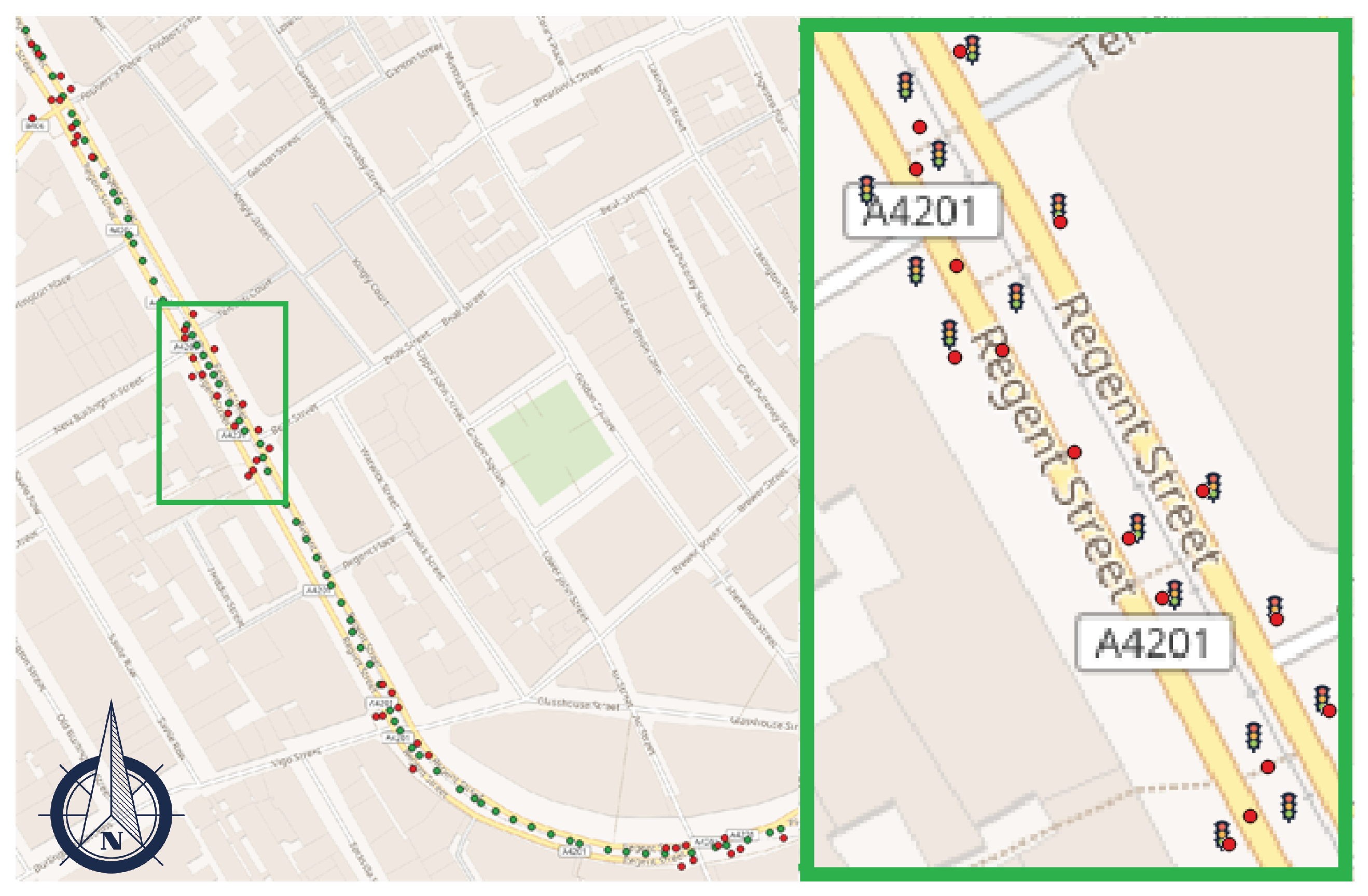
Figure 3.
Map of traffic lights automatically detected in Regent Street, London, UK. Green dots, red dots, and traffic light symbols (in zoom) are the GSV camera locations, geotagging results, and the actual locations of objects, respectively.
Figure 3.
Map of traffic lights automatically detected in Regent Street, London, UK. Green dots, red dots, and traffic light symbols (in zoom) are the GSV camera locations, geotagging results, and the actual locations of objects, respectively.

Figure 4.
Traffic light segmentation on Google Street View images. First row: correct segmentation. Second row: noisy or incomplete segmentation. Third row: false negative (left) and false positives.
Figure 4.
Traffic light segmentation on Google Street View images. First row: correct segmentation. Second row: noisy or incomplete segmentation. Third row: false negative (left) and false positives.

Figure 5.
Multiple views of detected traffic lights positions: each observed from four distinct GSV camera locations with view headings calculated based on the camera’s and estimated object’s coordinates. The field of view in each of four image comprising multi-view panel is , of which the central are between the yellow vertical lines.

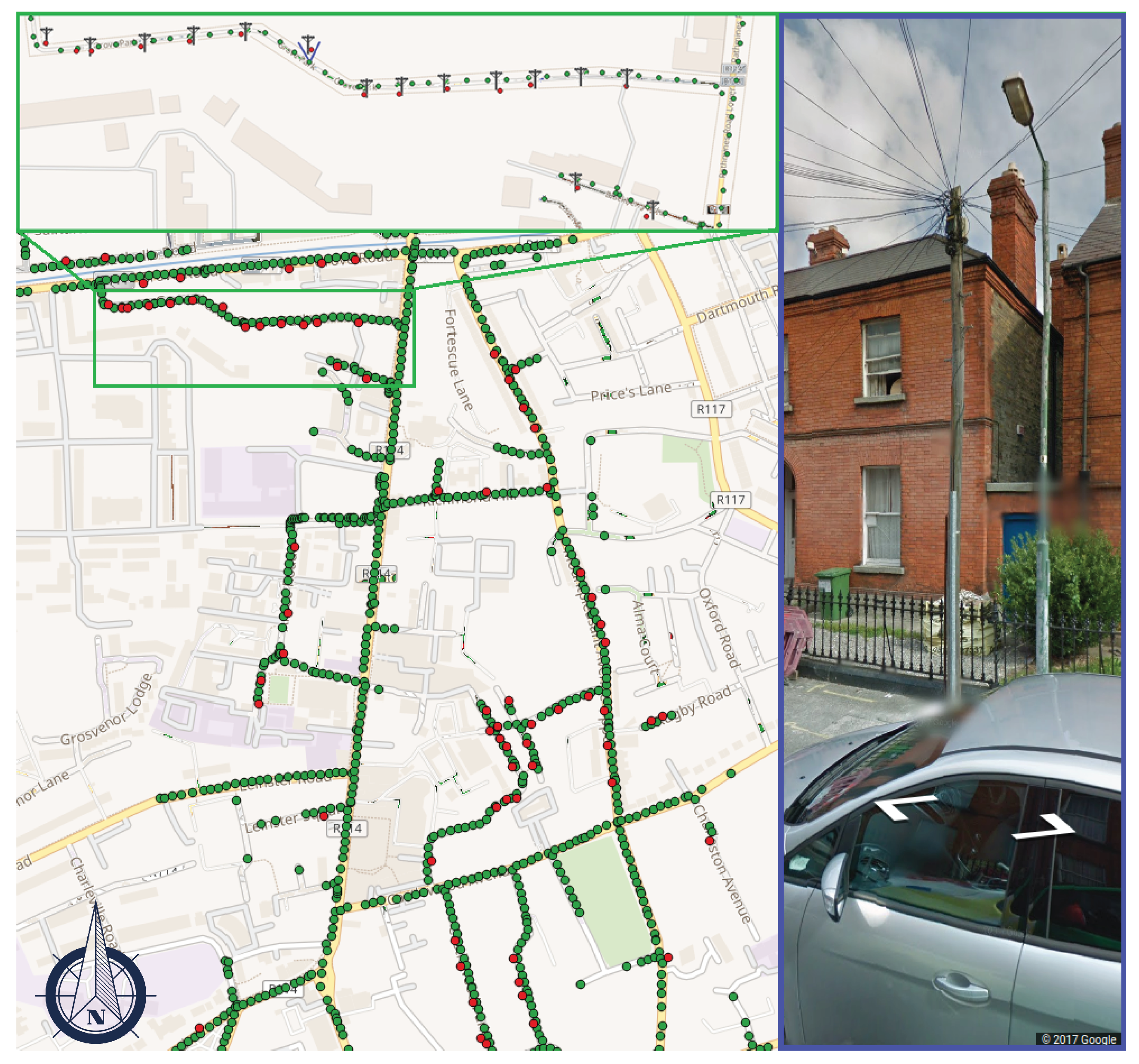
Figure 6.
Map of telegraph poles detected in Dublin, Ireland. Green dots, red dots, and pole symbols (in zoom) are the GSV camera locations, detected and actual locations of objects, respectively. The image in blue is a GSV image of one of the poles with image position and geo-orientation set up based on our geotag estimate.

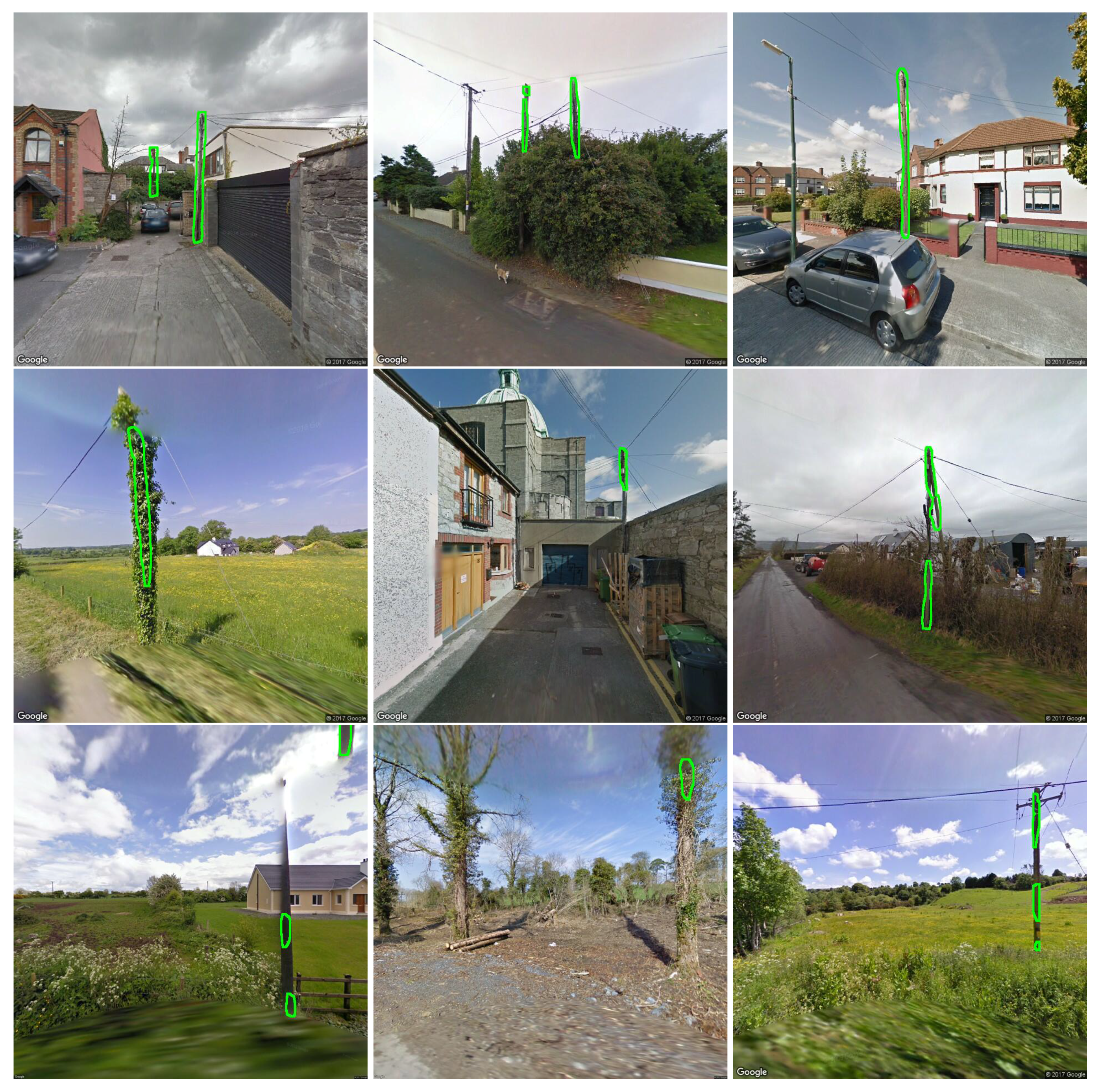
Figure 7.
Telegraph pole segmentation on Google Street View (GSV) images. First row: correct segmentation. Second row: partial detection. Third row: poor detection due to strong stitching (left) and false positives: ivy-covered tree and electricity pole.
Figure 7.
Telegraph pole segmentation on Google Street View (GSV) images. First row: correct segmentation. Second row: partial detection. Third row: poor detection due to strong stitching (left) and false positives: ivy-covered tree and electricity pole.


Table 1.
Instance-level object discovery results for traffic lights and telegraph poles in the test areas.
Table 1.
Instance-level object discovery results for traffic lights and telegraph poles in the test areas.
| Extent | #Actual | #Detected | True Positives | False Positives | False Negatives | Recall | Precision | ||
|---|---|---|---|---|---|---|---|---|---|
 | 0.8 km | 50 | 51 | 47 | 4 | 3 | 0.940 | 0.922 | |
 | Study A | 8 km | 77 | 75 | 72 | 3 | 5 | 0.935 | 0.960 |
 | Study B | 120 km | 2696 | 2565 | 2497 | 68 | 199 | 0.926 | 0.973 |
Table 2.
Accuracy of localization: distance statistics in meters from reference data collected on site with a GPS receiver.
Table 2.
Accuracy of localization: distance statistics in meters from reference data collected on site with a GPS receiver.
| Method | Mean | Median | Variance | 95% e.c.i. |
|---|---|---|---|---|
| MRF-triangulation | 0.98 | 1.04 | 0.65 | 2.07 |
| depth FCNN | 3.2 | 2.9 | 2.1 | 6.8 |
© 2018 by the authors. Licensee MDPI, Basel, Switzerland. This article is an open access article distributed under the terms and conditions of the Creative Commons Attribution (CC BY) license (http://creativecommons.org/licenses/by/4.0/).
Share and Cite
MDPI and ACS Style
Krylov, V.A.; Kenny, E.; Dahyot, R. Automatic Discovery and Geotagging of Objects from Street View Imagery. Remote Sens. 2018, 10, 661. https://doi.org/10.3390/rs10050661
AMA Style
Krylov VA, Kenny E, Dahyot R. Automatic Discovery and Geotagging of Objects from Street View Imagery. Remote Sensing. 2018; 10(5):661. https://doi.org/10.3390/rs10050661
Chicago/Turabian StyleKrylov, Vladimir A., Eamonn Kenny, and Rozenn Dahyot. 2018. "Automatic Discovery and Geotagging of Objects from Street View Imagery" Remote Sensing 10, no. 5: 661. https://doi.org/10.3390/rs10050661
Note that from the first issue of 2016, this journal uses article numbers instead of page numbers. See further details here.