Remote Sensing of Suspended Sediment Concentrations Based on the Waveform Decomposition of Airborne LiDAR Bathymetry


1
School of Geodesy and Geomatics, Wuhan University, 129 Luoyu Road, Wuhan 430079, China
2
Institute of Marine Science and Technology, Wuhan University, Wuhan 430079, China
3
Automation Department, School of Power and Mechanical Engineering, Wuhan University, Wuhan 430072, China
4
The Survey Bureau of Hydrology and Water Resources of Yangtze Estuary, Shanghai 200136, China
*
Author to whom correspondence should be addressed.
Remote Sens. 2018, 10(2), 247; https://doi.org/10.3390/rs10020247
Submission received: 6 January 2018
/
Revised: 1 February 2018
/
Accepted: 3 February 2018
/
Published: 6 February 2018
(This article belongs to the Section Ocean Remote Sensing)
Abstract
:Airborne LiDAR bathymetry (ALB) has been shown to have the ability to retrieve water turbidity using the waveform parameters (i.e., slopes and amplitudes) of volume backscatter returns. However, directly and accurately extracting the parameters of volume backscatter returns from raw green-pulse waveforms in shallow waters is difficult because of the short waveform. This study proposes a new accurate and efficient method for the remote sensing of suspended sediment concentrations (SSCs) in shallow waters based on the waveform decomposition of ALB. The proposed method approaches raw ALB green-pulse waveforms through a synthetic waveform model that comprises a Gaussian function (for fitting the air–water interface returns), triangle function (for fitting the volume backscatter returns), and Weibull function (for fitting the bottom returns). Moreover, the volume backscatter returns are separated from the raw green-pulse waveforms by the triangle function. The separated volume backscatter returns are used as bases to calculate the waveform parameters (i.e., slopes and amplitudes). These waveform parameters and the measured SSCs are used to build two power SSC models (i.e., SSC (C)-Slope (K) and SSC (C)-Amplitude (A) models) at the measured SSC stations. Thereafter, the combined model is formed by the two established C-K and C-A models to retrieve SSCs. SSCs in the modeling water area are retrieved using the combined model. A complete process for retrieving SSCs using the proposed method is provided. The proposed method was applied to retrieve SSCs from an actual ALB measurement performed using the Optech Coastal Zone Mapping and Imaging LiDAR in a shallow and turbid water area. A mean bias of 0.05 mg/L and standard deviation of 3.8 mg/L were obtained in the experimental area using the combined model.
1. Introduction
Suspended sediments play a major role in erosion/deposition processes, biomass primary production, and the transport of nutrients, micropollutants, and heavy metals [1]. Thus, reliable and spatially distributed observations of suspended sediment concentrations (SSCs) should be acquired to advance our understanding of the biogeomorphic dynamics of estuarine and lagoon systems and to develop effective and quantitative monitoring schemes [1]. In situ point measurements and optical remote sensing are common measurement techniques for SSCs. The in situ point measurements performed through gravimetric analysis directly produce accurate SSCs. The information obtained from filtered sediments is often considered the true concentration used for the calibration of other methods [2]. Despite the accuracy of this method, the cost and time related to the acquisition of these water samples are high and the necessary logistics are quite complex, thereby resulting in a sample distribution that is limited in time and space [3].
Optical remote sensing is often adopted to obtain spatial–temporal changes in SSC efficiently [1,4]. Optical remote sensing involves passive and active methods. Passive methods generally use spectrometers on satellites to measure the radiance entering the aperture of the sensor. SSCs can be retrieved through passive remote sensing provided that sufficient in situ ancillary information for appropriate calibration is available [1]. The literature validated the feasibility of applying radiometric data from satellites to estimate SSCs [1,3,5,6,7,8,9]. The estimation of SSCs through passive remote sensing is quite developed but generally concerns deep marine coastal waters; low–resolution sensors are often unsuitable for applications in estuaries and lagoons [1].
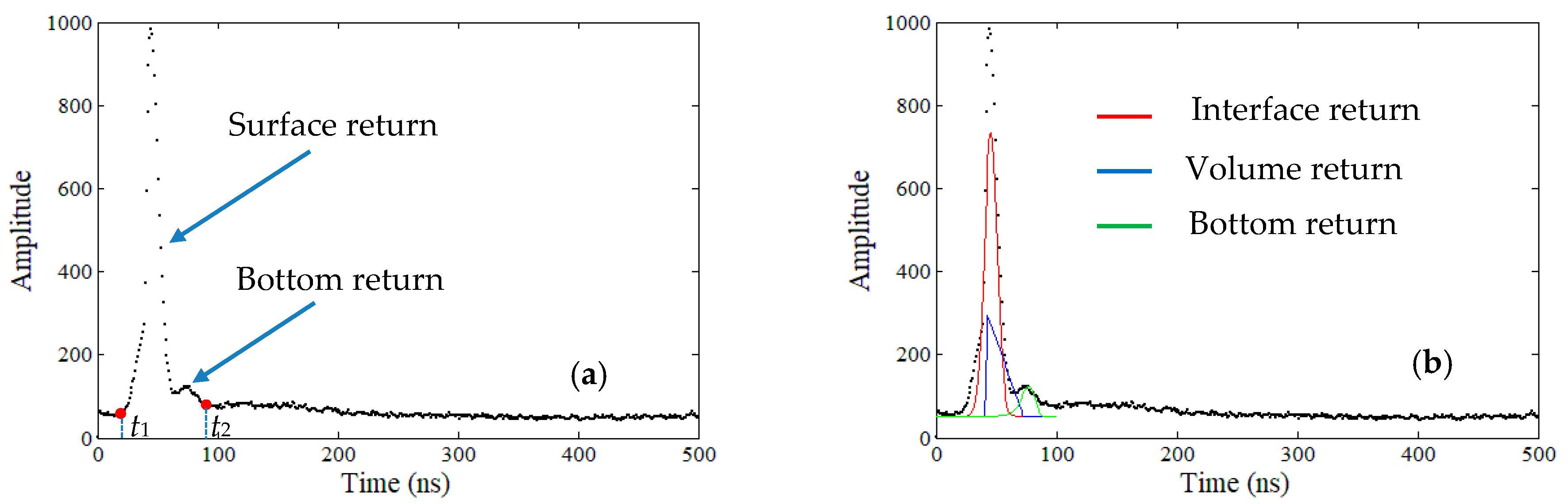
In contrast to passive optical remote sensing methods, active methods generally employ laser illumination (e.g., airborne LiDAR bathymetry (ALB)), avoiding the problems associated with reliance on the sun and low-resolution, and can operate at night and in shallow waters [10]. ALB is an accurate, cost-effective, and rapid technique for shallow water measurements [11,12,13] and can also be used for non-bathymetric purposes, such as the measurement of seawater turbidity [14]. Although water turbidity depends on SSCs and particle composition, many experiments have shown a good linear relationship between water turbidity and SSCs [12]. Thus, the turbidity estimated using ALB can be used as an indirect method to obtain SSCs. At present, ALB systems are tested to characterize the water turbidity of the upper water column by using green-pulse waveforms [4,11,15,16]. The loss of volume backscatter return depends on the turbidity of a body of water. Conversely, an analysis of the decay of the recorded waveform signal enables estimation of turbidity [16]. In general, such parameters as amplitude and slope of the column backscatter related to attenuation are estimated from pulse waveforms to retrieve water turbidity [11,15]. The relationship between water turbidity and the parameters estimated from raw waveforms has been investigated and has demonstrated the capability of ALB to detect, map, and monitor water turbidity [17,18,19]. An exponential function [16] and a linear function [4] are used to fit the return waveform of the water column part in order to estimate water turbidity. These methods are simple, effective, and can directly extract the parameter of volume backscatter return from the raw pulse waveforms by utilizing the fitting functions. In the existing methods, the SSC estimation is based on situations in which the range of volume backscatter return is significantly long, thereby enabling the extraction of the amplitude and slope of volume backscatter returns from the raw pulse waveforms. However, estimations will become inefficient in shallow waters because the range of volume backscatter return is short or completely missing [4]. In Figure 1a, the volume backscatter return in the raw pulse waveform is long and the traditional parameter extraction method can be utilized. Nevertheless, the traditional method is ineffective in the situation that the volume backscatter return is missing in the raw waveform in shallow waters (Figure 1b). Therefore, we developed a new method for estimating SSCs from the shallow water ALB data based on waveform decomposition.
Green surface return is a linear superposition of the energy reflected from the actual air–water interface and the energy backscattered from the particulate materials in the water volume just under the interface [11]. In our study, the volume backscatter return is extracted from the raw pulse waveform through waveform decomposition. According to the correlation between the volume backscatter return and measured SSC, SSC is retrieved by establishing an empirical SSC model, that is, the functions relating the slope and amplitude of volume backscatter return to measured SSCs. This paper is structured as follows. Section 2 provides the theoretical basis of the proposed method. Section 3 validates and analyzes the proposed method through experiments. Section 4 provides the corresponding discussions. Section 5 presents the conclusions and recommendations obtained from the experiments and discussions.
2. Method
2.1. Parameters of the Volume Backscatter Return
(a) Slope of the volume backscatter return
The LiDAR equation in the water column can be expressed as follows based on the description of Allocca et al. (2002) [15] and Collin et al. (2008) [20]:
where P(t) is the received power of the bathymetric LiDAR signal at time t; W is the constant combining loss; PT is the transmitted power; R is the bottom reflectance; Ksys is the system attenuation coefficient related to water clarity; and h is the in-water propagation distance.
The following equation that is linear in depth can be obtained by transforming Equation (1) using a natural log:
The system attenuation coefficient Ksys can be calculated as follows:
where t1 and t2 are the two adjacent times, and cwater is the propagation velocity of the green laser in water. The diffuse attenuation coefficient Kd is a predictor of water clarity [11]. The waveform-calculated system attenuation coefficient Ksys is related not only to Kd but also to ALB parameters, such as field of view (FOV) [11,21,22]. If the receiver FOV is sufficient, then Ksys approaches Kd [22,23,24]. In our study, we assumed that the FOV of the Coastal Zone Mapping and Imaging LiDAR (CZMIL) was large enough to collect all the returning energy to the receiver unit, and Ksys approached Kd.
The powers of laser returns (P) are detected by the detectors, usually photomultiplier tubes (PMTs) or avalanche photodiodes (APDs) [25,26]. Realistically, the expected dynamic range of the LiDAR returns is large and spans approximately several decades [25]. Therefore, a logarithmic amplifier [26] or a dynode bias circuit [27] is used to produce an effective logarithmic electrical response to compress the signal before it is delivered to the analog to digital converter (ADC). The outputs of detectors are digitized using high-speed ADCs at 1 GHz (1 ns/sample) to produce the waveforms (Amp) required for ranging measurements [25]. The raw waveform derived by the ADC is a semi-log plot with a logarithmic scale on the y-axis (amplitude) and a linear scale on the x-axis (time (ns)) (Figure 1). This process can be expressed as follows:
where Amp is the amplitude of the waveform, α is a scaling constant, and P is the power of laser returns.
Figure 1 shows that the volume backscatter slope K in the raw-pulse waveform can be defined as follows:
where A(t1) and A(t2) are the waveform amplitudes at times t1 and t2; and the corresponding powers are P(t1) and P(t2), respectively.
From Equations (3) and (5), we can derive the equation that K is directly proportional to Ksys.
Ksys is related to water turbidity, and the slope K is proportional to Ksys. If K can be obtained, then SSC can be retrieved by building an empirical model between K and SSC.
(b) Amplitude of the volume backscatter return
Guenther [26] described a general expression for the mean peak air–water interface return power as follows:
where θ is the beam scanning angle; N(θ, w) is the normalized Cox–Munk wave-slope distribution; w is the wind speeds; η is the total system optical efficiency; PT is the transmitted peak laser power; SR is the aperture area of the receiver telescope; H is the sensor height; and ρs(w) is the effective surface reflectivity per unit solid angle. The magnitude of the volume backscatter power can be written in the following form:
where nw is the index of refraction of water; σ is the volume-scattering function; Ksys is a system attenuation coefficient related to the water clarity and receiver field of view; t is time; and ρv(σ,Ksys,t) is the backscatter reflectivity per unit solid angle of the water column.
Equation (7) shows that surface waves have significant effects on the air–water interface return power Ps and that Ps is independent of water turbidity. Equation (8) shows that surface waves have no significant effect on the magnitude Pv of the volume backscatter power [26], and Pv is related to the system attenuation coefficient Ksys, which in turn is related to the diffuse attenuation coefficient Kd. Therefore, we can retrieve SSC through Pv. As is mentioned in Equation (4), Pv can be transferred into the waveform amplitude by inputting Pv into an ADC, thereby enabling the retrieval of SSC by building a model between the amplitude of volume backscatter return and the measured SSC. However, the received surface return is the linear supposition of the air–water interface return and volume backscatter return. The amplitude of volume backscatter return can only be obtained by separating the volume backscatter return from the raw-pulse waveform.
2.2. Waveform Decomposition
Figure 2 shows that a typical bathymetric LiDAR waveform comprises the surface return, volume backscatter return, bottom return, and background noise level [11]. The surface return is a linear superposition of the energy reflected from the actual air–water interface and the energy backscattered from particulate materials in the water volume just under the interface. Previous studies are based on the assumption that the range of volume backscatter return in deep waters is significantly long (Figure 1a) and the parameters of volume backscatter return can be extracted accurately from the raw green-pulse waveform. The longer the volume backscatter return is, the more accurately the waveform parameters can be estimated from the raw pulse waveform influenced by noises from the environment and ALB instruments. Kim [4] pointed out that a significantly long range of the slant distance (more than 18.7 m) makes possible the good estimation of average attenuation. Assuming that the ADC sampling rate is 1 ns/sample, 1 ns corresponds to about 0.15 m in slant distance. Conversely, a slant distance of 18.7 m corresponds to 125 samples of volume backscatter return in the raw waveform. However, if the volume backscattering range is short or missing, the estimated Ksys would be quite inaccurate using the traditional waveform analysis method (Figure 1b) [4].
If the volume backscatter returns can be separated accurately from the superposed surface returns and its waveform range (b–c in Figure 2) can be enlarged relative to that in the raw waveform (t1–t2 in Figure 2), then the parameters of volume backscatter returns can be estimated from the green-pulse waveform for retrieving SSCs (Figure 1b and Figure 2). Waveform decomposition is widely used in ALB depth estimation [28,29,30]. The advantage of this method is that it can extract the air–water interface return and volume backscatter return from the superposed surface return in the raw green waveform based on the waveform characteristics of various components of the return.
Ceccaldi [31] tested the combinations of several functions to efficiently distinguish the waveform contributions. Of all the functions considered, Gaussian, triangle, and Weibull functions have been verified to yield a high performance in fitting the air–water interface, the volume backscatter and the bottom returns, respectively [31]. Abady et al. [32] replaced the triangle function with a quadrilateral function to fit volume backscatter returns and assessed the method by using waveforms simulated by a Water LiDAR (Wa-LID) waveform simulator. Wa-LID was developed to simulate the reflection of LiDAR waveforms from water across visible wavelengths [33]. Although the accuracy of quadrilateral function is slightly better than that of the triangle function [32], the number of parameters used in the former (six parameters) is more than that used in the latter (four parameters) and thus increase the complexity of waveform decomposition. Schwarz et al. [34] proposed an exponential decomposition method that uses a model composed of segments of exponential functions to fit waveforms and considers the influence of system waveforms. This method can undo the blurring of a differential backscatter cross section caused by a laser sensor and result in a stable estimation of the water surface [34]. The quadrilateral function and the exponential decomposition need to be verified further by a lot of ALB data and water turbidity information. To conduct a simple and efficient decomposition, the method in reference [31] is adopted in this study.
As is shown in Figure 2, the air–water interface return, IR, can be expressed by a Gaussian function as follows:
where t is the time; As is the amplitude of the air–water interface return; μs is the time position of the surface (ns); and σs is the standard deviation. The volume backscatter return VB can be depicted by the triangle function as follows:
where Ac is the amplitude of volume backscatter return and (a, b, c) denote the time positions of the triangle vertices. The bottom return BR can be expressed by a Weibull function as follows:
where Ab is the amplitude of the bottom return, λb is the time position of the bottom return, and kb is the shape parameter.
The green waveform model GM comprising the air–water interface return, volume backscatter return, bottom return, and background noise level e can be depicted as follows:
Using the received raw green-pulse waveforms, the parameters (i.e., As, μs, σs, Ac, a, b, c, Ab, λb, kb) in the combination function (Equation (12)) can be estimated using a non-linear least–squares (NLS) approach using the Levenberg–Marquardt optimization algorithm. The Levenberg–Marquardt algorithm is an iterative procedure, and its primary application is in the least-squares curve fitting problem [35]. Given a set of m empirical datum pairs (xi, yi) of independent and dependent variables, we calculated the parameters β of the model curve f(x, β) so that the sum of the squares of the deviations S(β) was minimized as follows:
After obtaining VB(t, Ac, a, b, c), the amplitude A of volume backscatter return can be calculated as follows:
The slope K of volume backscatter return can be calculated on the basis of the assumption of homogeneous water turbidity in the vertical direction as follows:
2.3. Empirical Suspended Sediment Concentration (SSC) Models
After obtaining K and A of the volume backscatter return, SSC (C) can be estimated by building empirical models, namely, a C-K model between C and K and/or a C-A model between C and A.
(a) C-K model
The slopes of volume backscatter returns are related to Kd and can be used to retrieve SSC. We can build the following C-K relationship model based on the calculated slopes at SSC sampling stations:
(b) C-A model
The amplitudes A of volume backscatter returns are related to Kd and can be used to retrieve SSC. Similarly, we can build the C-A relationship model as follows:
Through the C-K and the C-A models, SSCs at a pulse spot can be estimated by using K and A, respectively, of the corresponding volume backscatter return.
(c) Combined SSC model
Through the C-K and C-A models, we can obtain the two solutions of C at a position. To obtain a single and robust C at a position, a combined model which is the linear combination of the C-K and C-A models is given as follows:
where k is an weighting coefficient that ranges from 0 to 1. The SSC error matrix V of all pulse spots in the representative water is as follows:
where
where n is the total pulse numbers in the representative water and Cmeasured is the measured SSC of the SSC sampling station. The value of the weight k can be solved using the least square method as follows:
2.4. Remote Sensing of SSCs Based on the Waveform Decomposition of Airborne LiDAR Bathymetry (ALB)
Figure 3 shows the process for remote sensing of SSCs in a measurement area using the preceding methods. Six steps comprise the retrieval process.
Step 1: Waveforms of green pulses are extracted from the raw binary data files.
Step 2: The volume backscatter returns are separated from the green waveforms through the waveform decomposition described in Section 2.2.
Step 3: The slopes Ks and amplitudes As of volume backscatter returns are calculated using the separated volume backscatter returns.
Step 4: The C-K and C-A models are built using Ks, As and the measured Cs at all SSC sampling stations.
Step 5: The final retrieval SSC model is formed by combining the established C-K and C-A models.
Step 6: SSC of each pulse spot is estimated by inputting K and A of the corresponding volume backscatter return into the combined SSC model.
3. Experiment and Analysis
3.1. Data Acquisition
A comprehensive survey was conducted in December 2014 in a shallow coastal water area with high turbidity and varying depths of 2–6 m (near Lianyungang, Jiangsu Province, China) to evaluate the reliability and accuracy of the proposed method. The eight strips of ALB data were collected using the CZMIL. Table 1 lists the primary technical parameters of CZMIL. Suspended sediment sampling was conducted in the same water area. Four suspended sediment-sampling stations were arranged around the survey area (Figure 4). During the ALB measurement, seawater samples were collected using horizontal water samplers in situ and analyzed in the laboratory. Each water sample was filtered, dried, and weighed. Suspended-sediment sampling was performed only in the surface, middle, and bottom layers at each sampling station. The mean value of SSCs measured at different layers was used as a representative SSC for each sampling station because of slight SSC changes. The assumption of homogeneous water turbidity in the vertical direction was adopted during SSC measurements. Figure 4 shows the locations and scopes of the different measurements. Table 2 lists the representative SSCs of the four sampling stations.
3.2. Building the SSC Models
(1) Waveform Decomposition
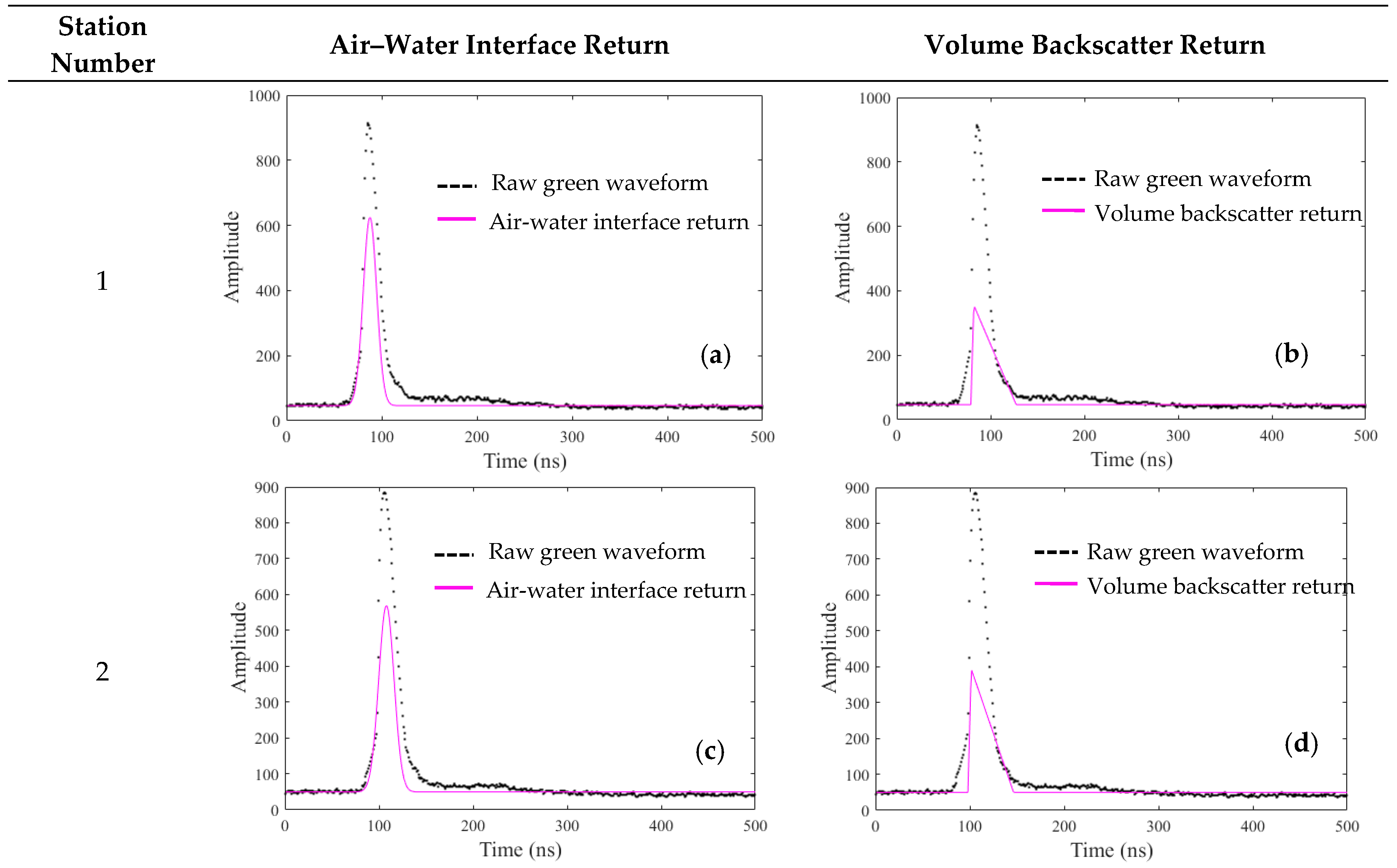
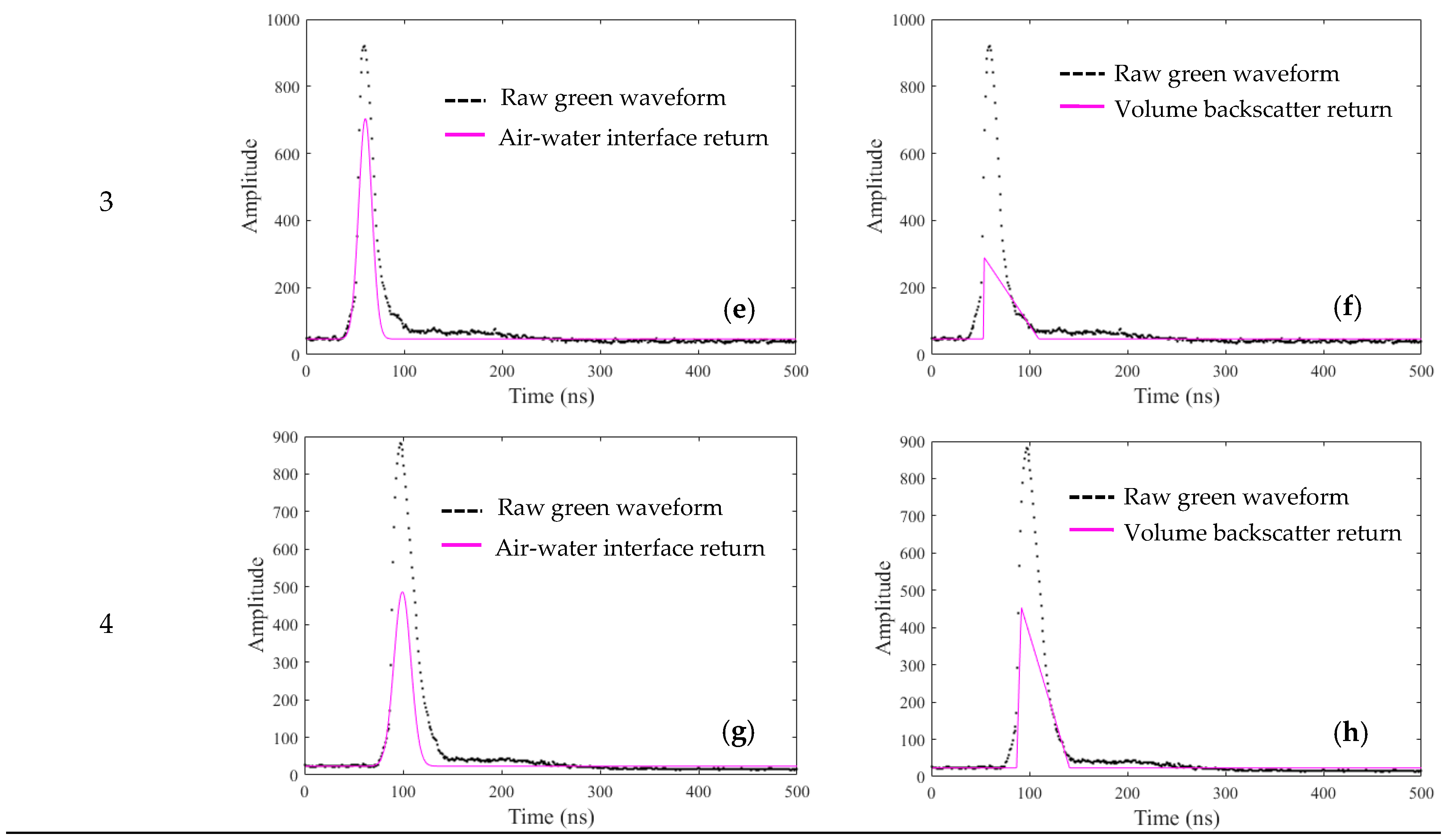
The 100 m × 100 m water area around each sampling station was selected as a representative sampling domain. In the four representative locations, 6011 pulse waveforms derived from the deep channel of CZMIL were extracted from the raw binary waveform files. Figure 5 shows several raw waveforms in each representative water area. The air–water interface return and volume backscatter return are superposed as the green surface return. Accordingly, distinguishing the volume backscatter return from the raw pulse waveform is difficult because of the short waveform range. The bottom return probably cannot be obtained in the raw waveforms because its amplitude is less than the background noise in the high water turbidity. To obtain the accurate slopes and amplitudes of volume backscatter returns, the waveform decomposition method depicted in Section 2.2 was adopted. The volume backscatter returns are separated from the superposed surface returns by establishing the green waveform model (see Equation (12)) using the raw waveforms. The green waveform model enables formation of the waveforms of the air–water interface returns (see Figure 5a,c,e,g) and corresponding volume backscatter returns (see Figure 5b,d,f,h). To ensure the accuracy of the separated volume backscatter waveform, the established green waveform model is assessed by comparing the sum of the two separated waveforms and raw waveform. Table 3 lists the statistical parameters of the model residuals in the four representative waters. The standard deviations in the four representative waters are below 20.5. Pearson’s correlation coefficient R2 between the raw waveform and the sum of the air–water interface return and the volume backscatter return is 0.995. The high R2 and low residuals (see Figure 5 and Table 3) show that the combination of Gaussian and triangle functions fit the green surface return well and that the volume backscatter return can be extracted accurately from the green surface return. The accuracy of the waveform decomposition can be assessed further based on the consistencies of Ks (or As) of the separated volume backscatter returns in a representative area. At a representative area, the biases of K and A of each pulse shot can be calculated by referring to the means of Ks and As of all pulse shots in the area. Table 4 lists the corresponding statistical parameters of the two types of biases. The standard deviations of Ks and As in the four representative waters are below 0.43 and 18.8, respectively. These results show that consistent Ks (or As) in a representative area can be derived from the separated volume backscatter returns and further verifies the feasibility of the proposed waveform decomposition method for extracting the volume backscatter return from the green surface return.
(2) Built SSC Models Using the Parameters of Volume Backscatter Return
Given the spatial distribution of the four SSC sampling stations, the slopes and amplitudes of volume backscatter returns and SSCs at stations 1, 3, and 4 are used to build the C-K, C-A and combined models.
(a) Empirical C-K model
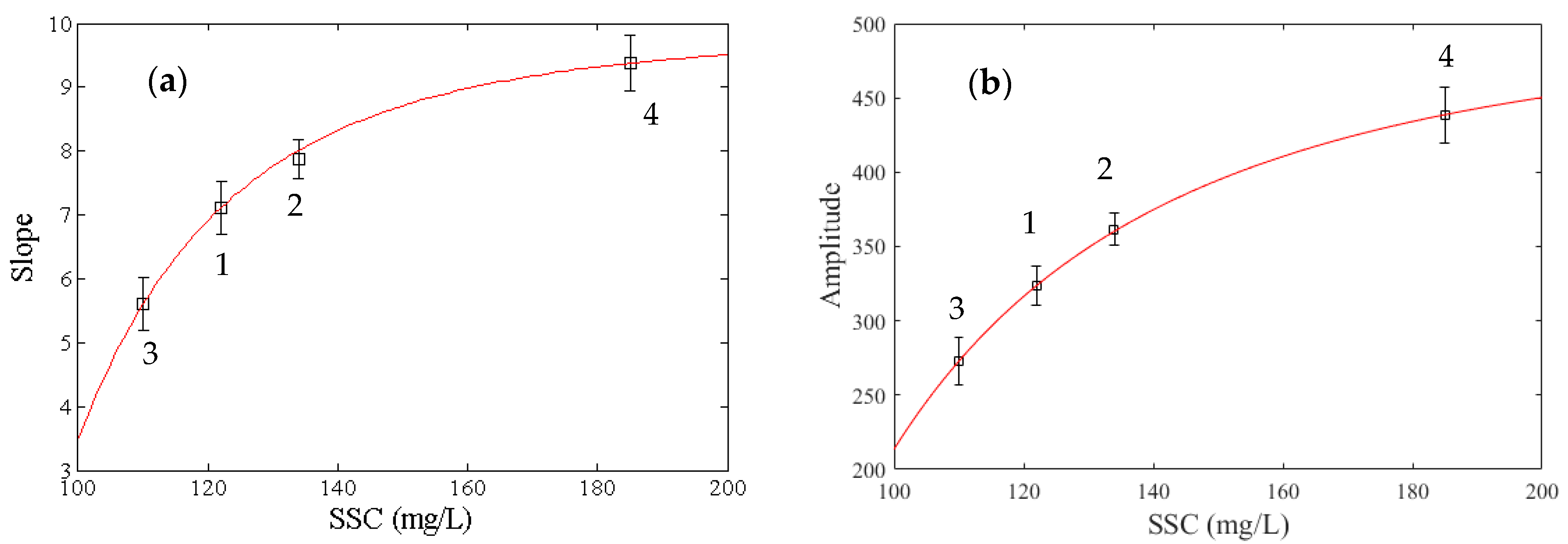
Figure 6a shows that the relationship between the slopes of volume backscatter returns and measured SSCs in the four representative waters is monotonically increasing. On the basis of this variation, the following power function is used to estimate SSC variations:
where C denotes SSC, K is the slope of volume backscatter return, and a1, b1, and c1 are the model coefficients. The model coefficients are estimated using the NLS method. Table 5 lists the results. The Pearson’s correlation coefficient R2 of the C-K model is 0.86. Figure 6a shows the regression curve formed by the C-K model. The high R2 and Figure 6a show that the C-K model fits the measured SSCs well.
(b) Empirical C-A model
Figure 6b shows that the relationship between the amplitudes of volume backscatter returns and measured SSCs in the four representative waters is also monotonically increasing. Similarly, a power function is given to estimate SSCs:
where A is the amplitude of volume backscatter return; and a2, b2, and c2 are the model coefficients. The coefficients are estimated using the NLS method (see Table 5). The Pearson’s correlation coefficient R2 of the C-A model is 0.89. Figure 6b shows the regression curve of the C-A model. The high R2 and Figure 6b show that the power function fits the measured SSCs well.
(c) Empirical combined SSC model
To build a robust estimation model, the combined SSC model depicted as Equation (18) is built by combining the estimated C-K and C-A models. The weight value k is solved using the process depicted in Equations (19)–(22) and determined as 0.15:
(3) Accuracy Analysis
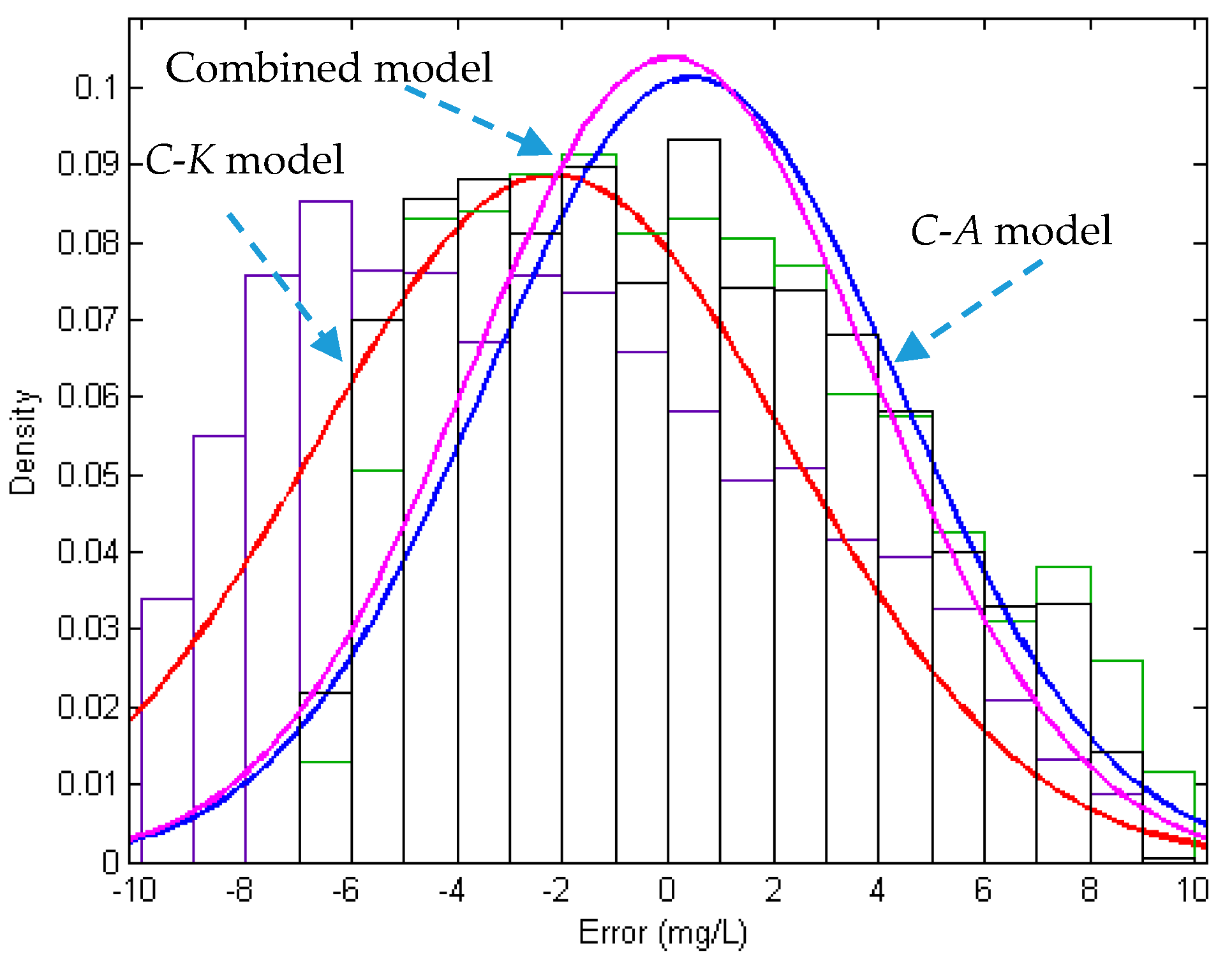
In our experiment, the data at stations 1, 3, and 4 were used to build the SSC models. The Pearson’s correlation coefficient R2 (Table 5) is used to reflect the goodness of fit. R2 can also indicate the internal accuracies of the established SSC models at stations 1, 3, and 4. The SSCs at each pulse spot of the representative water area of station 2 are estimated with the established C-K, C-A, and combined model, respectively. SSC measured in situ at station 2 can be used as an external reference to assess the accuracies of the three models. Figure 7 and Table 6 show the probability density distribution (PDF) and statistical parameters of SSC bias. The standard deviation of the SSC bias achieved by the combined model is less than those achieved by the C-K and C-A models. In addition, the means of the SSC biases achieved by the combined and C-A models are approximately zero and significantly less than those by the C-K model. The mean of the C-K model biases is −2.2 mg/L, which shows a systematic error in the C-K model. This statistical result indicates that the combined model has better performance in retrieving SSC than the single C-K or C-A models.
3.3. Remote Sensing of SSCs
SSCs at each pulse spot of the measured water area are estimated using the three SSC models.
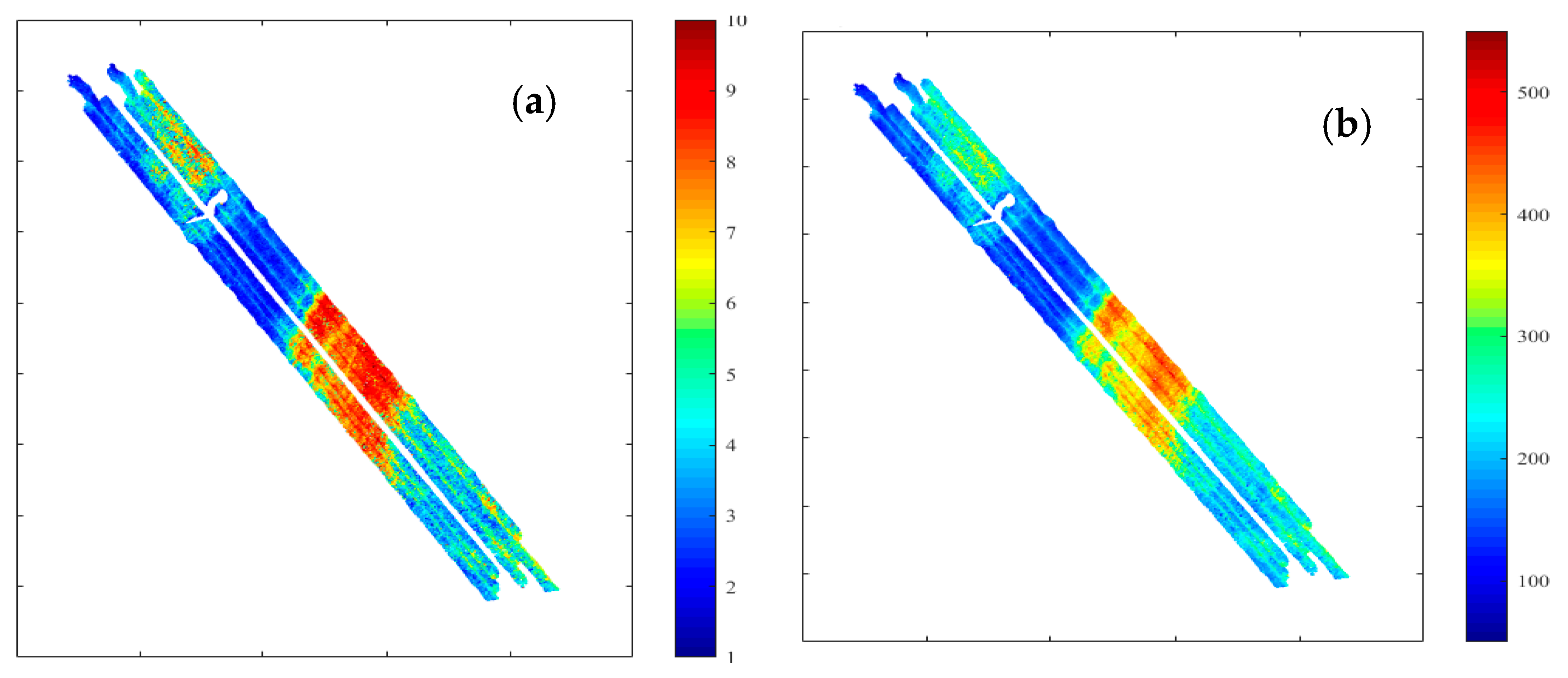
(1) A total of 76,776 green pulse waveforms from seven strips acquired using the deep channel of CZMIL are extracted from the raw binary waveform data files. The waveform decomposition method is applied to separate the volume backscatter returns from such pulse waveforms. The slopes and amplitudes of the separated volume backscatter returns are calculated (see Figure 8a,b, respectively). The slopes in the experimental water area range from 1.5 to 9.6 and the amplitudes range from 65 to 466. Figure 8 shows regional transitional variations of Ks and As resulting from the SSC changes. This example shows the feasibility of establishing a retrieval model with Ks and As of the volume backscatter returns.
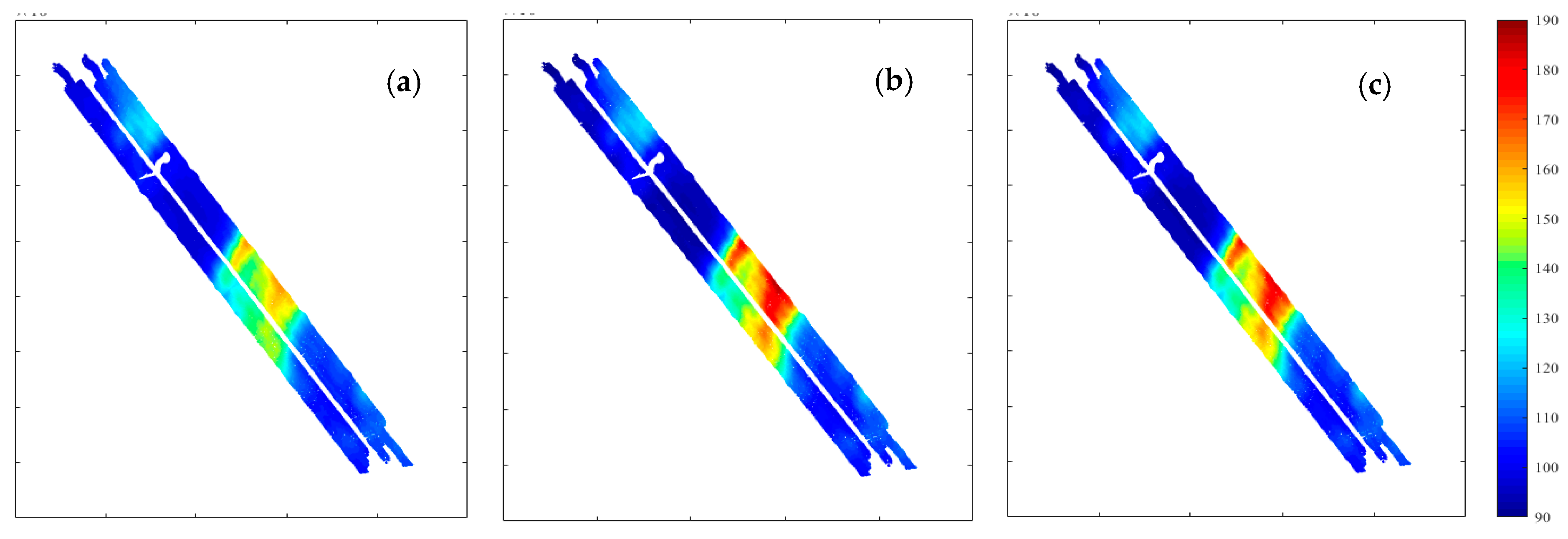
(2) SSCs of each pulse spot in the experimental water area are estimated using the established C-K, C-A, and combined SSC models by inputting the corresponding K and A. A moving average method is used to filter noises induced by the errors of calculated waveform parameters. Figure 9 shows the distributions of SSCs estimated using the different SSC models. SSCs estimated using the C-K model vary from 96 mg/L to 162 mg/L, those using the C-A model vary from 89 mg/L to 186 mg/L, and those using the combined SSC model vary from 90 mg/L to 182 mg/L. The distributions of SSCs estimated using the different SSC models have high consistency. Given that the combined model has higher accuracy than the C-K and C-A models, the SSC retrieved by the combined model is used as the final result.
4. Discussion
The proposed approach provides a good method for the remote sensing of SSCs in shallow waters based on waveform decomposition of ALB. The accuracy of the estimated SSCs in the study area is related to the slope and amplitude of volume backscatter return separated by the waveform decomposition and the constructed SSC models.
(a) Advantage of the proposed method
Traditional methods directly extract the slope and amplitude from the water column parts of raw green-pulse waveforms to retrieve water turbidity in deep water. However, accurately obtaining these parameters in shallow water is difficult when the range of volume backscatter return in the green-pulse waveform is short or missing. The waveform decomposition is a good tool to separate the volume return from the raw green waveform. The proposed method overcomes the shortcoming of traditional methods and can extract the volume backscatter return from the raw pulse waveform to accurately retrieve SSC in shallow waters. The range of the separated volume backscatter return (Figure 5b,d,f,h) is enlarged relative to that in the raw green waveform. The stretching is beneficial for accurately calculating the slopes and amplitudes of volume backscatter returns, as well as retrieving SSC. To conveniently obtain these waveform parameters, 18 m of water depth is defined as a limitation based on current knowledge and previous studies [4]. When the ALB depth is below 18 m, the waveform decomposition should be adopted in the extraction of the waveform parameters and SSC retrieval. Otherwise, the traditional method is adopted.
(b) Performance of the waveform decomposition
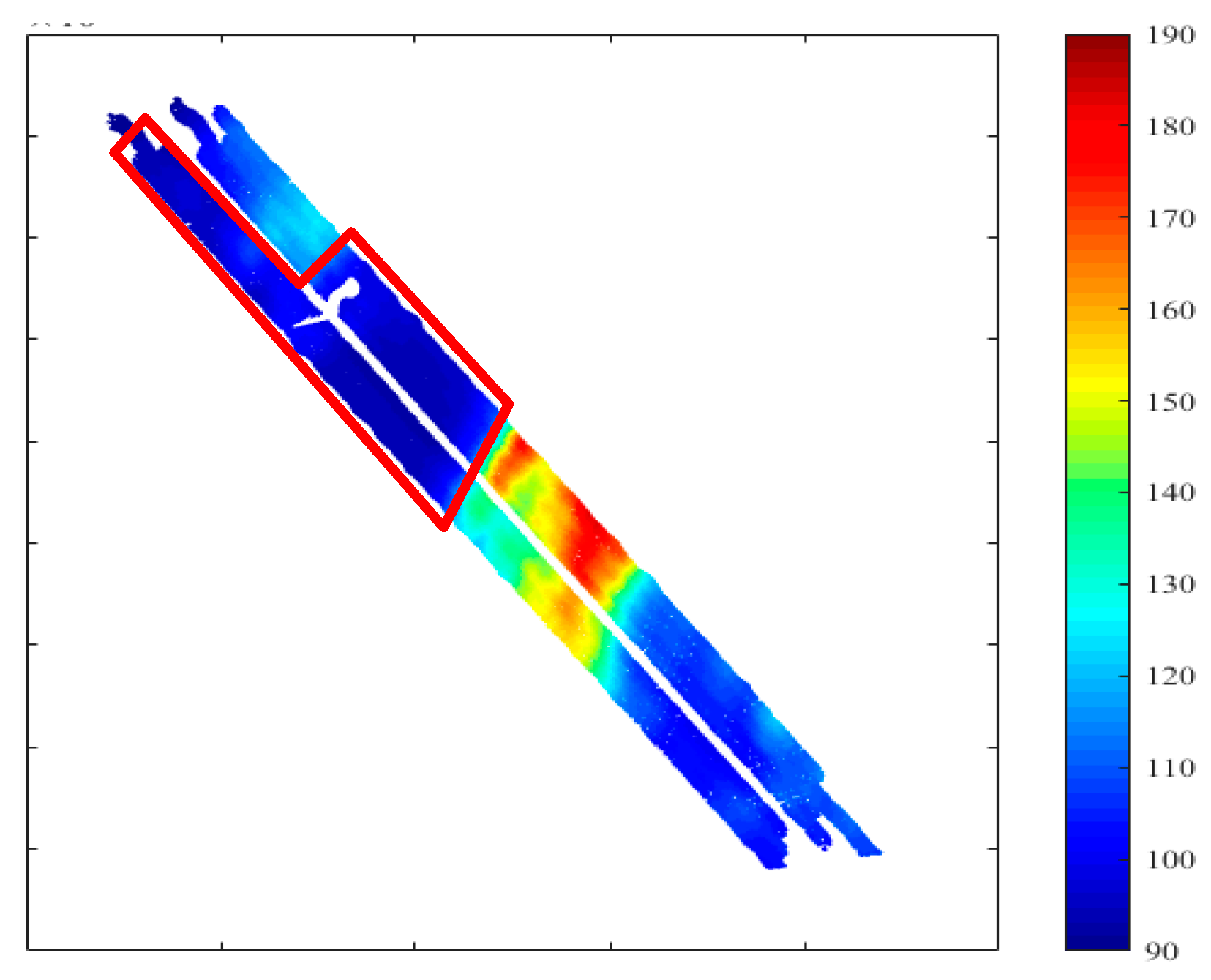
In Section 3.2, the accuracy of waveform decomposition was assessed in four SSC sampling stations in terms of residuals, R2, and consistency of the parameters calculated from separated volume backscatter returns. The bottom returns are missing in all of the sampling stations because of high water turbidity, but this will not always be the case if the water is shallower and/or less turbid. So the waveform decomposition should also be assessed using the waveforms with distinct bottom returns. In Figure 10, the bottom returns can be found in an area with low-turbid water. In such an area, the retrieved SSCs are less than 90 mg/L and far less than the SSCs in other areas. This result is consistent with the actual situation and verifies the efficiency of the waveform decomposition and the SSC retrieval models. A total of 1333 pulse waveforms with distinct bottom returns are detected in this water area. The waveform-decomposition methods described in Section 2.2 are assessed by these pulse waveforms. One typical raw waveform with distinct bottom returns is shown in Figure 11a, and the corresponding waveform-decomposition results are illustrated in Figure 11b. Only waveforms between the leading edge of the surface return and the tailing edge of the bottom return are assessed because other parts of the waveforms are useless signals induced by noises of the environment and the ALB instrument (Figure 11a). The maximum, minimum, mean, and standard deviation of the residuals are 67.5, −26.3, 3.9 and 17.5, respectively. R2 between the raw waveform and the sum of the three returns is 0.99. The high R2 and low residuals indicate that waveform decomposition can also be applied to waveforms with distinct bottom returns.
(c) Initial values of waveform decomposition
Our experiment validated the effectiveness of the proposed waveform-decomposition method in the experimental water area with shallow water depth and high turbidity. The water depth determines the time range of volume backscatter return and amplitude of the bottom return, while the water turbidity determines the amplitudes of the volume backscatter and bottom returns. Although the key parameters of volume backscatter return (i.e., Ac, a, b, c) and bottom return (i.e., Ab, λb, kb) can be estimated through the NLS approach using the Levenberg–Marquardt optimization algorithm, initial values of these parameters given by the prior water depth and turbidity of the measured water area will accelerate the convergence rate of the non-linear least-square fitting. The prior water depth can be calculated using water surface height and water bottom height determined by ALB. Prior turbidity can be obtained by interpolating SSC using field measurements.
(d) Retrieving SSC models
This study constructed three empirical SSC models (i.e., the C-K, C-A, and combined models) using the slopes and amplitudes of the separated volume backscatter returns. The models were built using the dataset collected by CZMIL in shallow and turbid waters. In other waters or data collected using other ALB systems, the three models should be rebuilt to enable the SSC retrieval model, established by the measured waveform parameters, to fit well with the actual SSCs in the water body of interest.
The C-K, C-A, and combined models reflect the SSC in the measurement water. In the above experiment, the C-A model is better than the C-K model and makes a larger contribution to the combined model. Meanwhile, the combined model is best among the three. Because the combined model is built using the slopes and amplitudes of volume returns and the measured SSCs, the combined model can weaken the shortcomings of the C-K and C-A models and is robust.
(e) Application
The proposed method addressed the issue of accurately retrieving SSC in shallow waters. The method also can be applied in deep waters. In situ point measurements of SSC should be performed to calibrate the waveform parameters derived from the raw pulse waveforms. To ensure the accuracy of the proposed method, the density and representativeness of the SSC sampling stations should be considered when collecting these field data.
5. Conclusions and Suggestions
This study proposed a novel method for remote sensing of SSC based on waveform decomposition of ALB. The proposed method overcomes the shortcoming of traditional methods and can extract the volume backscatter return from the raw pulse waveform to accurately retrieve SSC in shallow waters. Experiments verified the proposed methods. The experimental results show that the volume backscatter returns can be efficiently separated from the raw pulse waveforms using the waveform decomposition method. The SDs of the slopes and amplitudes of the separated volume backscatter returns in the four representative waters of the SSC sampling stations were below 0.43 and 18.8, respectively. Three retrieving SSC models (i.e., the C-K, C-A and combined models) were built using the waveform parameters and measured SSCs. SDs of 4.5, 3.9, and 3.8 mg/L were obtained using the C-K, C-A, and combined models, respectively, thereby showing that the combined model was best among the three models. SSC in the measurement water was obtained using the combined model.
The proposed method is also suitable for retrieving SSC in deep water. Our experiment was conducted in shallow and turbid waters with four SSC sampling stations for the calibration. Further tests should be performed in similar waters with more SSC sampling stations.
Acknowledgments
This research is supported by the National Natural Science Foundation of China (Coded by 41376109, 41176068, and 41576107) and the National Science and Technology Major Project (Coded by 2016YFB0501703). The data used in this study were provided by the Survey Bureau of Hydrology and Water Resources of the Yangtze Estuary. The authors are grateful for their support.
Author Contributions
Jianhu Zhao, Hongmei Zhang, and Xinglei Zhao developed and designed the experiments; Fengnian Zhou and Xinglei Zhao performed the experiments; Jianhu Zhao, Hongmei Zhang, and Xinglei Zhao analyzed the data; Jianhu Zhao, Hongmei Zhang, and Xinglei Zhao wrote the paper.
Conflicts of Interest
The authors declare no conflict of interest.
References
- Volpe, V.; Silvestri, S.; Marani, M. Remote sensing retrieval of suspended sediment concentration in shallow waters. Remote Sens. Environ. 2011, 115, 44–54. [Google Scholar] [CrossRef]
- Guillén, J.; Palanques, A.; Puig, P. Field calibration of optical sensors for measuring suspended sediment concentration in the western Mediterranean. Sci. Mar. 2000, 64, 427–435. [Google Scholar] [CrossRef] [Green Version]
- Montanher, O.C.; Novo, E.M.; Barbosa, C.C. Empirical models for estimating the suspended sediment concentration in Amazonian white water rivers using Landsat 5/TM. Int. J. Appl. Earth Obs. Geoinf. 2014, 29, 67–77. [Google Scholar] [CrossRef]
- Kim, M.; Feygels, V.; Kopilevich, Y.; Park, J.Y. Estimation of inherent optical properties from CZMIL lidar. In Proceedings of the SPIE Asia-Pacific Remote Sensing, Beijing, China, 13–16 October 2014; Volume 9262, p. 92620W. [Google Scholar]
- Curran, P.J.; Novo, E.M. The relationship between suspended sediment concentration and remotely sensed spectral radiance: A review. J. Coast. Res. 1998, 4, 351–368. [Google Scholar]
- Warrick, J.A.; Mertes, L.A.K.; Siegel, D.A.; Mackenzie, C. Estimating suspended sediment concentrations in turbid coastal waters of the Santa Barbara Channel with SeaWiFS. Int. J. Remote Sens. 2004, 25, 1995–2002. [Google Scholar] [CrossRef]
- Binding, C.E.; Bowers, D.G.; Mitchelson-Jacob, E.G. Estimating suspended sediment concentrations from ocean colour measurements in moderately turbid waters; the impact of variable particle scattering properties. Remote Sens. Environ. 2005, 94, 373–383. [Google Scholar] [CrossRef]
- Wang, J.J.; Lu, X.X. Estimation of suspended sediment concentrations using Terra MODIS: An example from the Lower Yangtze River, China. Sci. Total Environ. 2010, 408, 1131–1138. [Google Scholar] [CrossRef] [PubMed]
- Giardino, C.; Bresciani, M.; Valentini, E.; Gasperini, L.; Bolpagni, R.; Brando, V.E. Airborne hyperspectral data to assess suspended particulate matter and aquatic vegetation in a shallow and turbid lake. Remote Sens. Environ. 2015, 157, 48–57. [Google Scholar] [CrossRef]
- Gao, J. Bathymetric mapping by means of remote sensing: Methods, accuracy and limitations. Prog. Phys. Geogr. 2009, 33, 103–116. [Google Scholar] [CrossRef]
- Guenther, G.C.; Cunningham, A.G.; Laroque, P.E.; Reid, D.J. Meeting the accuracy challenge in airborne Lidar bathymetry. In Proceedings of the 20th EARSeL Symposium: Workshop on Lidar Remote Sensing of Land and Sea, Dresden, Germany, 16–17 June 2000. [Google Scholar]
- Zhao, J.; Zhao, X.; Zhang, H.; Zhou, F. Shallow Water Measurements Using a Single Green Laser Corrected by Building a Near Water Surface Penetration Model. Remote Sens. 2017, 9, 426. [Google Scholar] [CrossRef]
- Zhao, J.; Zhao, X.; Zhang, H.; Zhou, F. Improved Model for Depth Bias Correction in Airborne LiDAR Bathymetry Systems. Remote Sens. 2017, 9, 710. [Google Scholar] [CrossRef]
- Wong, H.; Antoniou, A. Characterization and decomposition of waveforms for LARSEN 500 airborne system. IEEE Trans. Geosci. Remote Sens. 1991, 29, 912–921. [Google Scholar] [CrossRef]
- Allocca, D.; London, M.; Curran, T.; Concannon, B.; Contarino, V.M.; Prentice, J.; Kane, T.J. Ocean water clarity measurement using shipboard lidar systems. Proc. SPIE 2002, 4488, 106–114. [Google Scholar]
- Richter, K.; Maas, H.G.; Westfeld, P.; Weiß, R. An Approach to Determining Turbidity and Correcting for Signal Attenuation in Airborne Lidar Bathymetry. PFG–J. Photogramm. Remote Sens. Geoinf. Sci. 2017, 85, 31–40. [Google Scholar] [CrossRef]
- Saylam, K.; Brown, R.A.; Hupp, J.R. Assessment of depth and turbidity with airborne Lidar bathymetry and multiband satellite imagery in shallow water bodies of the Alaskan North Slope. Int. J. Appl. Earth Obs. Geoinf. 2017, 58, 191–200. [Google Scholar] [CrossRef]
- Billard, B.; Abbot, R.H.; Penny, M.F. Airborne estimation of sea turbidity parameters from the WRELADS laser airborne depth sounder. Appl. Opt. 1986, 25, 2080–2088. [Google Scholar] [CrossRef] [PubMed]
- Philips, D.M.; Abbot, R.H.; Penny, M.F. Remote sensing of sea water turbidity with an airborne laser system. J. Phys. D Appl. Phys. 1984, 17, 1749. [Google Scholar] [CrossRef]
- Collin, A.; Archambault, P.; Long, B. Mapping the shallow water seabed habitat with the SHOALS. IEEE Trans. Geosci. Remote Sens. 2008, 46, 2947–2955. [Google Scholar] [CrossRef]
- Feygels, V.I.; Wright, C.W.; Kopilevich, Y.I.; Surkov, A.I. Narrow-field-of-view bathymetrical lidar: Theory and field test. In Ocean Remote Sensing and Imaging II, Proceedings of the Optical Science and Technology, SPIE'S 48th Annual Meeting, San Diego, CA, USA, 3–8 August 2003; SPIE: Bellingham, WA, USA, 2003; Volume 5155, pp. 1–12. [Google Scholar]
- Feygels, V.I.; Kopilevich, Y.I.; Surkov, A.I. Airborne lidar system with variable-field-of-view receiver for water optical properties measurement. In Ocean Remote Sensing and Imaging II, Proceedings of the Optical Science and Technology, SPIE'S 48th Annual Meeting, San Diego, CA, USA, 3–8 August 2003; SPIE: Bellingham, WA, USA, 2003; Volume 5155, pp. 12–22. [Google Scholar]
- Guenther, G.C. Digital Elevation Model Technologies and Applications: The DEM User’s Manual; ASPRS Publications: Annapolis, MD, USA, 2007; pp. 253–320. [Google Scholar]
- Steinvall, O.K.; Koppari, K.R.; Karlsson, U.C. Experimental evaluation of an airborne depth-sounding lidar. In Lidar for Remote Sensing, Proceedings of the Environmental Sensing ’92, Berlin, Germany, 15–19 June 1992; SPIE: Bellingham, WA, USA, 1992; Volume 1714, pp. 108–127. [Google Scholar]
- Fuchs, E.; Tuell, G. Conceptual design of the CZMIL data acquisition system (DAS): Integrating a new bathymetric lidar with a commercial spectrometer and metric camera for coastal mapping applications. In Proceedings of the SPIE Defense, Security, and Sensing, Orlando, FL, USA, 5–9 April 2010; Society of Photo-Optical Instrumentation Engineers (SPIE): Bellingham, WA, USA, 2010. [Google Scholar]
- Guenther, G.C. Airborne Laser Hydrography: System Design and Performance Factors. Available online: http://shoals.sam.usace.army.mil/downloads/Publications/AirborneLidarHydrography.pdf (accessed on 25 February 2017).
- Tuell, G.; Barbor, K.; Wozencraft, J. Overview of the coastal zone mapping and imaging LiDAR (CZMIL): A new multi-sensor airborne mapping system for the US Army Corps of Engineers. In Algorithms Technol. Multispectral, Hyperspectral, Ultraspectral Imagery XVI, Proceedings of the SPIE Defense, Security, and Sensing, Orlando, FL, USA, 5–9 April 2010; SPIE: Bellingham, WA, USA, 2010; Volume 7695, p. 76950R. [Google Scholar]
- Hofton, M.A.; Minster, J.B.; Blair, J.B. Decomposition of laser altimeter waveforms. IEEE Trans. Geosci. Remote Sens. 2000, 38, 1989–1996. [Google Scholar] [CrossRef]
- Wagner, W.; Ullrich, A.; Ducic, V.; Melzer, T.; Studnicka, N. Gaussian decomposition and calibration of a novel small-footprint full-waveform digitising airborne laser scanner. ISPRS J. Photogramm. Remote Sens. 2006, 60, 100–112. [Google Scholar] [CrossRef]
- Wang, C.; Li, Q.; Liu, Y.; Wu, G.; Liu, P.; Ding, X. A comparison of waveform processing algorithms for single-wavelength LiDAR bathymetry. ISPRS J. Photogramm. Remote Sens. 2015, 101, 22–35. [Google Scholar] [CrossRef]
- Abdallah, H.; Bailly, J.S.; Baghdadi, N.N.; Saint-Geours, N.; Fabre, F. Potential of space-borne LiDAR sensors for global bathymetry in coastal and inland waters. IEEE J. Sel. Top. Appl. Earth Obs. Remote Sens. 2013, 6, 202–216. [Google Scholar] [CrossRef]
- Abady, L.; Bailly, J.S.; Baghdadi, N. Assessment of quadrilateral fitting of the water column contribution in lidar waveforms on bathymetry estimates. IEEE Geosci. Remote Sens. Lett. 2014, 11, 813–817. [Google Scholar] [CrossRef]
- Abdallah, H.; Baghdadi, N.; Bailly, J.S. Wa-LiD: A new LiDAR simulator for waters. IEEE Geosci. Remote Sens. Lett. 2012, 9, 744–748. [Google Scholar] [CrossRef] [Green Version]
- Schwarz, R.; Pfeifer, N.; Pfennigbauer, M.; Ullrich, A. Exponential Decomposition with Implicit Deconvolution of Lidar Backscatter from the Water Column. PFG–J. Photogramm. Remote Sens. Geoinf. Sci. 2017, 85, 159–167. [Google Scholar] [CrossRef]
- Marquardt, D.W. An algorithm for least-squares estimation of nonlinear parameters. J. Soc. Ind. Appl. Math. 1963, 11, 431–441. [Google Scholar] [CrossRef]
Figure 1.
(a) Raw green-pulse waveform measured with the Coastal Zone Mapping and Imaging LiDAR (CZMIL) in waters with 10 m depth. The volume backscatter return is long because of deep water. The bottom return is missing because of the high turbidity and deep water; (b) raw green-pulse waveform measured with CZMIL in shallow waters with 3 m depth. The bottom return is close to the surface return, and the volume backscatter return is missing because of shallow water.
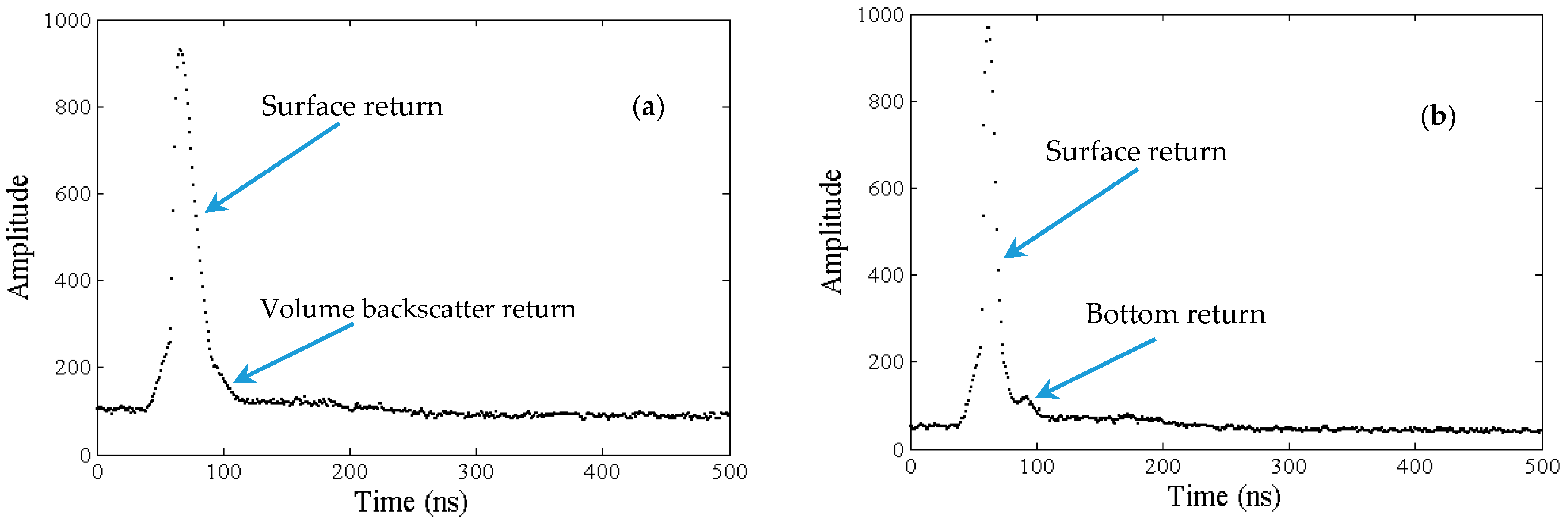
Figure 2.
Typical bathymetric LiDAR waveform composed of the air–water interface return, volume backscatter return, bottom return, and background noise. K and Ac denote the slope and amplitude of volume backscatter return, respectively, and e is the background noise level.
Figure 2.
Typical bathymetric LiDAR waveform composed of the air–water interface return, volume backscatter return, bottom return, and background noise. K and Ac denote the slope and amplitude of volume backscatter return, respectively, and e is the background noise level.
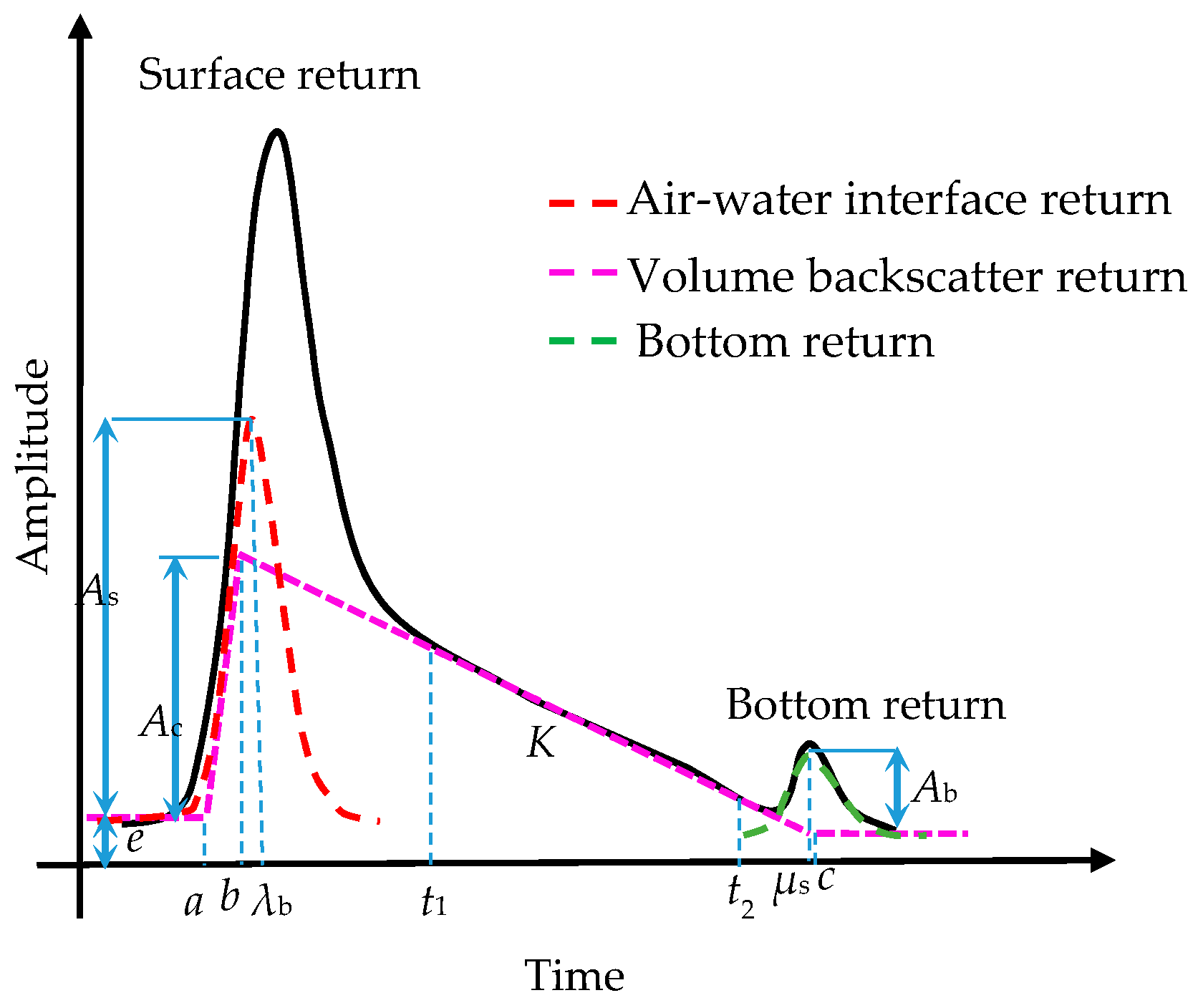
Figure 3.
Remote-sensing process of suspended sediment concentrations (SSCs) by the proposed method.
Figure 3.
Remote-sensing process of suspended sediment concentrations (SSCs) by the proposed method.
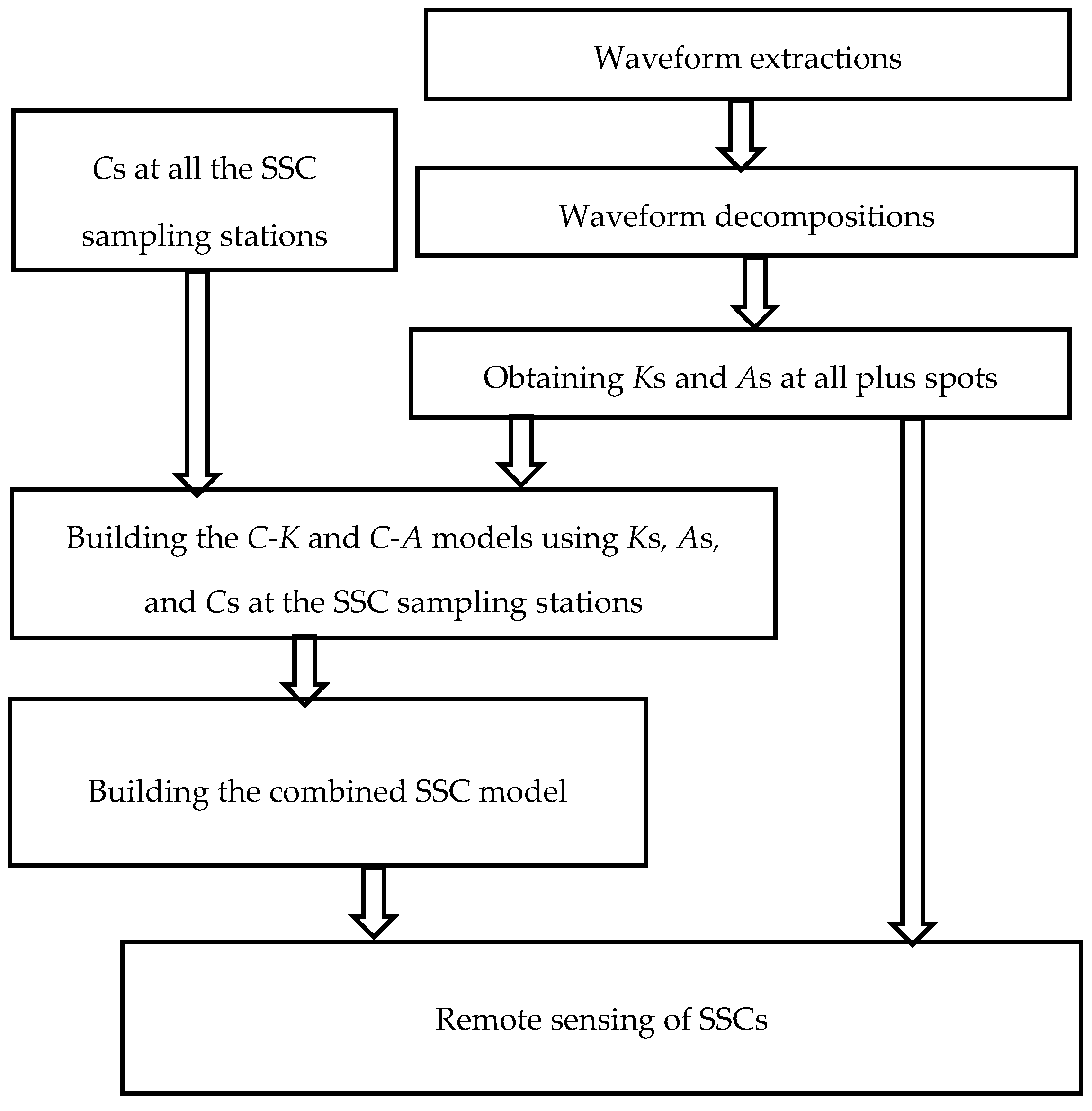
Figure 4.
Locations and scope of the different measurements. The yellow, red, and blue colors denote the land, scope of the airborne LiDAR bathymetry (ALB) measurement, and depth contours in the water area measured, respectively. 1–4 show the locations of the SSC sampling stations.
Figure 4.
Locations and scope of the different measurements. The yellow, red, and blue colors denote the land, scope of the airborne LiDAR bathymetry (ALB) measurement, and depth contours in the water area measured, respectively. 1–4 show the locations of the SSC sampling stations.
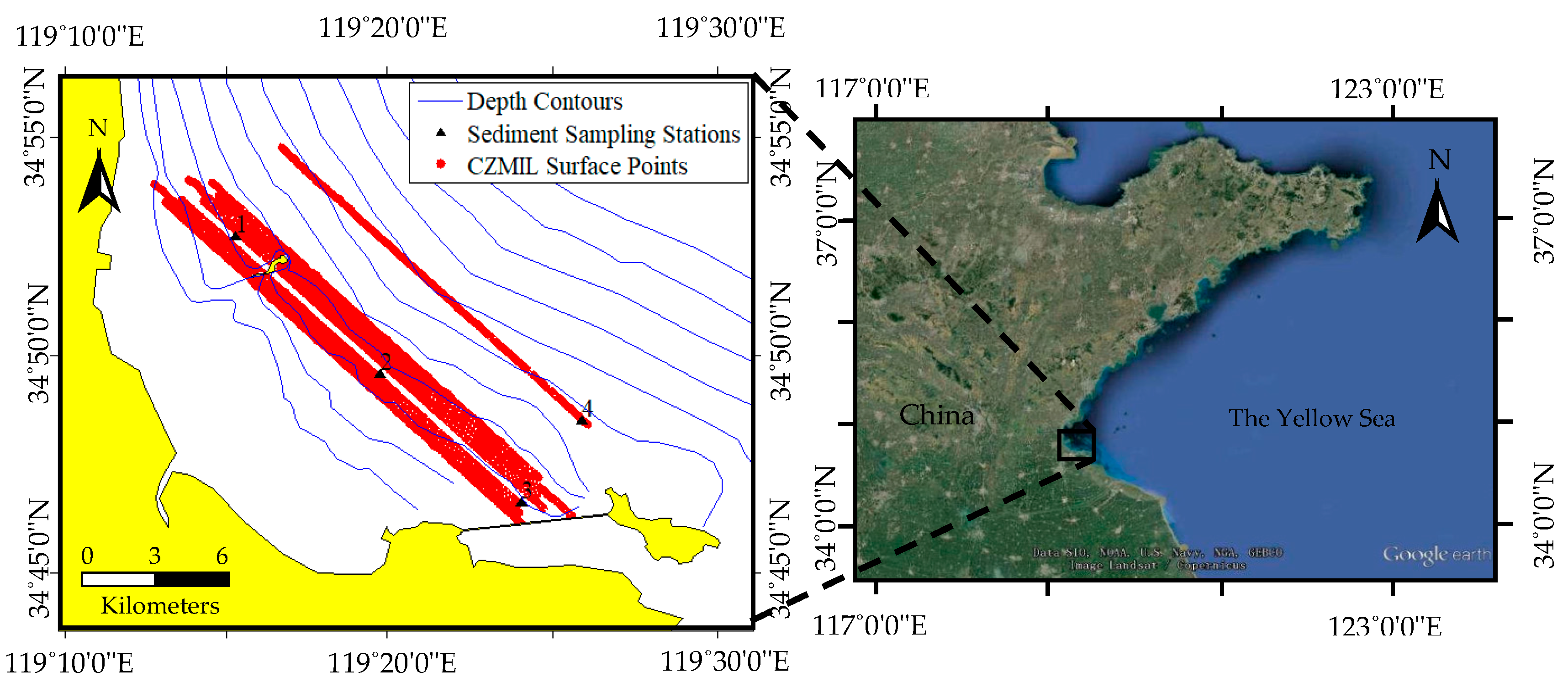
Figure 5.
Waveform decomposition in the four representative waters of the SSC sampling stations. (a,c,e,g) are the air–water interface returns separated by the waveform decomposition in the four representative waters. (b,d,f,h) are the corresponding volume backscatter returns separated by waveform decomposition in the four representative waters.


Figure 6.
(a) Relationship between the slopes and the measured SSCs in the four representative waters of the SSC sampling stations; (b) the relationship between the amplitudes and the measured SSCs in the four representative waters. 1–4 denote the SSC sampling stations. The center point and half-width of the error bar denote the mean and SD of the slope (amplitude), respectively. The red curves in (a,b) denote the regression lines of the C-K and C-A models.

Figure 7.
Probability density distribution of the SSC bias retrieved using the different models in the representative waters of sampling station 2.
Figure 7.
Probability density distribution of the SSC bias retrieved using the different models in the representative waters of sampling station 2.

Figure 8.
Slopes and amplitudes obtained using the proposed methods in the experimental water area. (a) Slopes of the separated volume backscatter returns; (b) corresponding amplitudes.
Figure 8.
Slopes and amplitudes obtained using the proposed methods in the experimental water area. (a) Slopes of the separated volume backscatter returns; (b) corresponding amplitudes.

Figure 9.
Distribution of SSCs estimated using the established C-K, C-A, and combined models in the experimental area. (a) Distribution of SSC estimated using the C-K model; (b) that using the C-A model; and (c) that using the combined SSC model.
Figure 9.
Distribution of SSCs estimated using the established C-K, C-A, and combined models in the experimental area. (a) Distribution of SSC estimated using the C-K model; (b) that using the C-A model; and (c) that using the combined SSC model.

Figure 10.
The red polygon denotes the water area with distinct bottom returns and the colorbar indicates the SSCs (mg/L) retrieved by the combined SSC model.
Figure 10.
The red polygon denotes the water area with distinct bottom returns and the colorbar indicates the SSCs (mg/L) retrieved by the combined SSC model.

Figure 11.
Waveform decomposition using a waveform with a distinct bottom return. (a) Raw waveform with a distinct bottom return. t1 and t2 denote the leading edge and tailing edge of the waveform, respectively; (b) extracted interface, volume and bottom returns determined through the waveform decomposition. The red curve denotes the air/water interface return, the blue curve denotes the volume backscatter return, and the green curve denotes the bottom return.

Table 1.
Technological parameters of the CZMIL system.
| Performance Index | Parameter |
|---|---|
| Operating altitude | 400 m (nominal) |
| Pulse repetition frequency | 10 kHz |
| Circular scan rate | 27 Hz |
| Laser wavelength | IR: 1064 nm; green: 532 nm |
| Maximum depth single pulse | Kd·Dmax = 3.75−4.0 daytime (bottom reflectivity >15%) |
| Minimum depth | <0.15 m |
| Depth accuracy | (0.32 + (0.013 depth)²)½ m, 2σ |
| Sounding scope | 0–30 m |
| Horizontal accuracy | (3.5 + 0.05 depth) m, 2σ |
| Scan angle | 20° (fixed off-nadir, circular pattern) |
| Swath width | 294 m (nominal) |
Table 2.
Representative SSCs of the different sampling stations.
| Station Number | SSC (mg/L) |
|---|---|
| 1 | 122 |
| 2 | 134 |
| 3 | 110 |
| 4 | 185 |
Table 3.
Statistical parameters of the model residuals of the green surface return in the four representative waters. SD means standard deviation. Unit: digitizer units.
Table 3.
Statistical parameters of the model residuals of the green surface return in the four representative waters. SD means standard deviation. Unit: digitizer units.
| Station Number | Pulse Numbers | Max. | Min. | Mean | SD |
|---|---|---|---|---|---|
| 1 | 1387 | 36 | −38 | –0.6 | 20.5 |
| 2 | 1044 | 25 | −32 | 0.6 | 17.2 |
| 3 | 1885 | 34 | −31 | −0.4 | 16.7 |
| 4 | 1695 | 29 | −36 | −0.2 | 16.8 |
Table 4.
Statistical parameters of the slopes and amplitudes estimated by waveform decomposition in the four representative waters. SD means standard deviation (1 sigma).
Table 4.
Statistical parameters of the slopes and amplitudes estimated by waveform decomposition in the four representative waters. SD means standard deviation (1 sigma).
| Station Number | Slope | Amplitude | ||||||
|---|---|---|---|---|---|---|---|---|
| Max. | Min. | Mean | SD | Max. | Min. | Mean | SD | |
| 1 | 7.99 | 6.26 | 7.11 | 0.42 | 350 | 300 | 324 | 13.4 |
| 2 | 8.43 | 7.31 | 7.87 | 0.30 | 382 | 342 | 361 | 10.7 |
| 3 | 6.45 | 4.64 | 5.60 | 0.42 | 300 | 232 | 273 | 16.1 |
| 4 | 9.44 | 8.49 | 9.38 | 0.43 | 480 | 397 | 439 | 18.8 |
Table 5.
Regression coefficients of the C-K and C-A models.
| C-K Model | C-A Model | ||||||
|---|---|---|---|---|---|---|---|
| a1 | b1 | c1 | R2 | a2 | b2 | c2 | R2 |
| −2.136 × 10⁹ | −4.263 | 9.839 | 0.86 | −1.556 × 10⁷ | −2.362 | 507.4 | 0.89 |
Table 6.
Statistical parameters of SSCs established using the different models in the representative waters of sampling station 2. SD means standard deviation.
Table 6.
Statistical parameters of SSCs established using the different models in the representative waters of sampling station 2. SD means standard deviation.
| Max. (mg/L) | Min. (mg/L) | Mean (mg/L) | SD (mg/L) | |
|---|---|---|---|---|
| C-K model | 8.5 | −9.8 | −2.20 | 4.5 |
| C-A model | 9.5 | −6.3 | 0.44 | 3.9 |
| Combined model | 9.0 | −6.6 | 0.05 | 3.8 |
© 2018 by the authors. Licensee MDPI, Basel, Switzerland. This article is an open access article distributed under the terms and conditions of the Creative Commons Attribution (CC BY) license (http://creativecommons.org/licenses/by/4.0/).
Share and Cite
MDPI and ACS Style
Zhao, X.; Zhao, J.; Zhang, H.; Zhou, F. Remote Sensing of Suspended Sediment Concentrations Based on the Waveform Decomposition of Airborne LiDAR Bathymetry. Remote Sens. 2018, 10, 247. https://doi.org/10.3390/rs10020247
AMA Style
Zhao X, Zhao J, Zhang H, Zhou F. Remote Sensing of Suspended Sediment Concentrations Based on the Waveform Decomposition of Airborne LiDAR Bathymetry. Remote Sensing. 2018; 10(2):247. https://doi.org/10.3390/rs10020247
Chicago/Turabian StyleZhao, Xinglei, Jianhu Zhao, Hongmei Zhang, and Fengnian Zhou. 2018. "Remote Sensing of Suspended Sediment Concentrations Based on the Waveform Decomposition of Airborne LiDAR Bathymetry" Remote Sensing 10, no. 2: 247. https://doi.org/10.3390/rs10020247
Note that from the first issue of 2016, this journal uses article numbers instead of page numbers. See further details here.