Article

Sensitivity and Limitation in Damage Detection for Individual Buildings Using InSAR Coherence—A Case Study in 2016 Kumamoto Earthquakes

1
Department of Electrical Engineering and Information Systems, The University of Tokyo, 7-3-1 Hongo, Bunkyo-ku, Tokyo 113-8656, Japan
2
Earth Observation Research Center, Japan Aerospace Exploration Agency, 2-1-1 Sengen, Tsukuba, Ibaraki 305-8505, Japan
3
Satellite Applications and Operations Center, Japan Aerospace Exploration Agency, 2-1-1 Sengen, Tsukuba, Ibaraki 305-8505, Japan
*
Author to whom correspondence should be addressed.
Remote Sens. 2018, 10(2), 245; https://doi.org/10.3390/rs10020245
Submission received: 4 December 2017 / Revised: 15 January 2018 / Accepted: 4 February 2018 / Published: 6 February 2018

Abstract

:
In this paper, evaluation results are presented for multi-temporal interferometric coherence analysis using a Synthetic Aperture Radar (SAR) for damage assessment in an urban area. The latest space-borne SARs potentially have a high enough spatial resolution to assess individual buildings. However, interferometric coherence analysis has not been evaluated for its limitation in sensitivity and size of damaged buildings. In particular, the correlation between the coherence analysis and the damage level referred to by architectural assessments has been an open question. In this paper, analytical results using ALOS-2 PALSAR-2 datasets are presented from the 2016 Kumamoto earthquakes in Japan. For reference, building damage was assessed throughout the central urban area and specifically at a catastrophically damaged district. The results show that the buildings should be larger than a window size of the coherence for damage detection, and the damage level should be larger than Level-2 of 5, classified with the European Macroseismic Scale 1998 (EMS-98).

Graphical Abstract

1. Introduction

Interferometric analyses using a synthetic aperture radar (Interferometric SAR, InSAR) have been widely used for detecting crustal deformation, ground subsidence, and landslides [1]. Not only the phase component of the interferogram, but also interferometric coherence, is used for disaster monitoring [2]. The SAR intensity images have been widely used for disaster monitoring in the same way as optical images [3,4]. On the other hand, interferometric coherence analysis requires frequent observations before and after the disaster, which was difficult to achieve in the early 2000s. When there are two pre-disaster datasets and one post-disaster image, the change in the interferometric coherence between the pre-disaster pairs and the co-disaster pairs can be calculated. The reduction of interferometric coherence in urban areas suggests the existence of damaged buildings. Compared to the intensity correlation, which has also been used for damage detection, the interferometric coherence-based change detection method has the advantage that it does not require a complete collapse of buildings. The change of SAR backscatter is derived by multiple reasons, including the change of the scattering mechanism. In urban areas, it is assumed to be caused by collapsed buildings because the buildings in urban areas rarely change their backscattering coefficient in multi-temporal observations. On the other hand, the SAR interferometric coherence decreases in urban areas mainly because the scattering points of the buildings are randomly deformed by the disaster. In other words, the change of interferometric coherence suggests rather moderate surface damage to the building. In short, the interferometric coherence change is potentially able to detect less damaged buildings compared to the intensity change.
Comparison between intensity and coherence change detection methods has been reported in various researches. For example, the 2003 Bam Iran earthquake showed the superiority of the coherence-based method in sensitivity, though both the ground truth data and the satellite data did not have a high enough spatial resolution [5,6,7]. One possible reason for insufficient ground truth data is that estimating the damage level of every building was of a low priority compared with rescuing and recovering operations. At the same time, the SAR analytical results did not have a high enough ground resolution to evaluate individual buildings. The SAR satellites which were launched in the early 2000s, e.g., ERS series, ENVISAT, and ALOS, had spatial resolutions larger than 10 m. The recent Sentinel-1 series applies the wide-swath TOPSAR mode in worldwide observations, resulting in an approximately 5 m × 20 m resolution. In these cases, a single building is equivalent to a few pixels in the SAR image and cannot be distinguished from the other buildings in the urban area. Thus, preceding studies could distinguish the damaged area within a scale of a city block, larger than thousands of square meters. In addition, some SAR satellites could not observe the affected area soon after the disaster occurred because of their limitation in observation schedules.
Polarimetric analysis (PolSAR) has been proposed to detect the change of scattering mechanism derived by the disaster [8]. PolSAR analysis was examined in, for example, 2011 off the pacific coast of the Tohoku Earthquake [9,10,11,12]. Current problems for this method are that there are less acquisitions for full polarimetric mode and less spatial resolution caused by the operational limit of the platforms.
Resent space-borne SARs, for example, TerraSAR-X, COSMO-SkyMed, RADARSAT-2, and ALOS-2, have resolutions smaller than 3 m in their Stripmap modes with flexible observation schedules. These satellites can potentially evaluate and detect the damage of an individual building soon after the disaster [13,14]. One problem with the high-frequency radars, such as X- and C-band SAR satellites, is their faster temporal decorrelation when compared to L-band SARs, resulting in a limited opportunity for multi-temporal interferometric coherence analysis. To avoid the effect of the temporal decorrelation, a larger filter and/or measuring a limited number of high coherency points are required. In urban areas, there is a limited effect of temporal decorrelation as buildings are stable and thus, X-/C-SARs can be applied for interferometric coherence analysis. There are also various reasons that reduce interferometric coherence such as liquefactions, landslides, and human activities including constructions [15]. Avoiding these causes for damage assessments in actual cases is required. In this article, we only evaluate the pixels that correspond to the building in Section 4. Some preceding researches reported the results for the comparison between SAR and optical observations among damaged buildings [3,4,8]. According to these researches, high-resolution SAR data can be used for evaluating the individual buildings if the interferometric pair has a high enough coherence.
On the other hand, L-band SAR has a slow temporal decorrelation, resulting in the requirement of a lower filter size [16]. In the case of previous L-band SARs, JERS-1, and ALOS, multi-temporal analyses could distinguish the damaged city blocks in the same manner as the higher-frequency SARs [17,18,19]. The latest L-band SAR satellite ALOS-2 has been observing the Earth since 2014 [20]. The Japan Aerospace Exploration Agency (JAXA) operates ALOS-2 to observe various disasters. Analytical results in the 2015 Nepal Gorkha Earthquake using ALOS-2 with the 10-m resolution mode suggested that a single building can be detected by interferometric analysis [21,22]. However, the 10-m resolution was too rough compared with the scale of the building. Thus, further analysis using higher resolution data has been demanded.
In short, there is an open issue that the coherence analysis has not been connected to the survey data using an architectural assessment scheme [23], e.g., European Macroseismic Scale 1998 (EMS-98) [24]. Especially for L-band SAR data, high-resolution interferometric coherence analyses have not been evaluated for their sensitivity in damage assessments. It has been an open question about how accurately ALOS-2 can evaluate damaged buildings with its 3-m resolution mode. For example, spatially distributed collapsed buildings caused by the 2016 Kumamoto earthquake were estimated by a temporal coherence decrease of the PALSAR-2 interferometric analysis over the earthquake, which has 58% accuracy against the spatial density of completely collapsed buildings inventoried by an in-situ survey [25]. This result, for example, suggests that the sensitivity of the temporal coherence decrease should be clarified in terms of the damage level and/or building size. If we could find the sensitivity and the limitation of the interferometric coherence analysis, we could perform a damage assessment for every building and facility [26].
In this paper, the change of the interferometric coherence in the ALOS-2 PALSAR-2 3-m resolution data is used to evaluate the potential of the L-band SAR for disaster monitoring and damage detection. The analytical results for the 2016 Kumamoto, Japan earthquakes [27,28] were compared with two independent observations. The first observation throughout a central urban area of Kumamoto considering a larger scale includes the aerial photography for counting the damaged buildings which are covered with plastic sheets. The second one, for a smaller scale, is the inventory survey based on EMS-98 in Mashikimachi town, a neighboring city of Kumamoto city which was severely damaged by the earthquakes.

2. Methodology

2.1. Multi-Temporal Interferometric Coherence

Interferometric coherence is the correlation of the complex signals between the two observations, namely “master” and “slave”. The interferometric coherence γ is calculated as:
γ = M S ¯ M M ¯ S S ¯
where M and S are the sample of master and slave single look complex images, respectively, and the bar above them denotes the complex conjugate. The brackets represent the ensemble average. If the ground surface has changed by the disaster, resulting in the phase randomness of the interferometric phase, its ensemble average in the specific window will be small. An insufficient window size will overestimate the coherence value, while the larger window size will reduce the ground resolution. The window size of the ensemble average in Equation (1) is 5 × 5 pixels in this article.
If we have at least one interferometric pair before the disaster occurs, we can compare the coherence value between pre- and co-event interferograms. If the co-event interferometric coherence is lower than the pre-event one, though considering temporal decorrelation, it can be regarded that scatterers on the surface have been largely damaged and/or moved. This is called multi-temporal interferometric coherence change detection. There are two major definitions of the coherence decrease between the pre-event coherence γpre and the co-event coherence γco. One is the simple difference or un-normalized coherence decrease (CD) un and the other is the normalized coherence decrease norm, as shown in Equations (2) and (3).
d γ u n = γ p r e γ c o
d γ n o r m = γ p r e γ c o γ p r e + γ c o
Equation (2) requires relatively large γpre and cannot be applied for low coherency areas, such as vegetated ground. On the other hand, Equation (3) does not require large γpre, while the temporal decorrelation will suffer in accuracy. In this article, we applied (2) because the buildings have large γpre. We excluded the vegetated area that may have low γpre for the evaluation and only evaluated buildings in our experiments in order to avoid false alarms.
In the damage detection scheme in this paper, a building will be regarded as damaged when un exceeds the specific threshold. The threshold is generally defined manually to reduce the effect of temporal and baseline decorrelations.

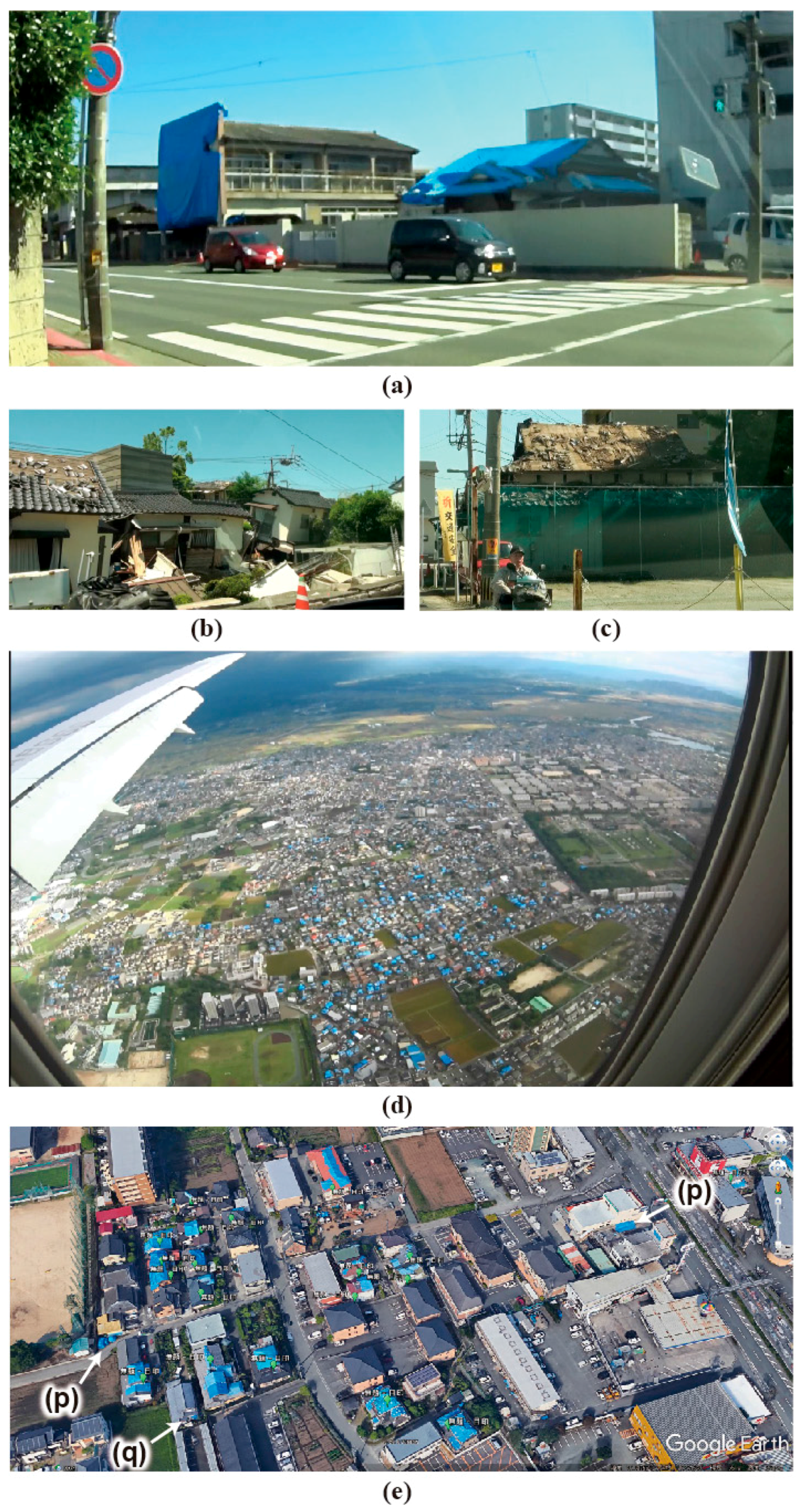
2.2. Aerial Photography Survey

We performed visual identification of damaged buildings using Google Earth around the central urban area of Kumamoto from 11 to 13 May 2016, as shown in Figure 1. This domain approximately ranges from 32˚45′ to 32˚50′N, and from 130˚40′ to 130˚50′E, inside the administrative district of Kumamoto city (A in Figure 1).
Numerous damaged buildings are covered with plastic sheets in blue, as shown in Figure 2. A plastic-sheet covering has the following roles:
  • To fix unstable parts to keep residents’ safe when walking around the building.
  • For thermal insulation to stop any air drafts from the damaged roof.
  • To avoid further damage by leaks caused by rain.
Therefore, buildings covered with plastic sheets imply that they sustained medium damage and still have a possibility of being repaired for continuous use. On the other hand, catastrophically damaged buildings (Figure 2b) and relatively old (~60 years) and damaged buildings (Figure 2c) are abandoned without any treatment, which implies demolition. Many of them are too dangerous to approach and are therefore controlled under prohibition of entry.
The blue sheets were easily identified from an airplane at a low altitude (<1000 m/3300 ft. a.s.l.) on the final approach course to Kumamoto airport (Figure 2d). Google Earth shows the same scenario with three-dimensional (3D) ground object models (Figure 2e) in a range within a rectangle of [32˚45′–32˚45′N, 130˚40′–130˚50′E], which is frequently seen in the central area of Kumamoto (Figure 1). These 3D models have been generated from a series of angled aerial photographs after the earthquake, which enables realistic high-resolution views from multiple angles. The basic technique uses areal imagery acquisition with a 45-degree off-nadir angle in multiple directions (e.g., [29]).
We recorded locations of the buildings with roofs covered with the plastic sheets in Google Earth (Figure 2e). We extracted all the buildings covered (completely or partially) with blue, white, or green sheets. Multiple sheets for one building are counted at one time. Plastic sheets covering other objects (i.e., external equipment, greenhouse, car, tombstone, and the ground) are excluded (e.g., (p) in Figure 2e). Covering of lined walls is excluded (e.g., (q) in Figure 2a,e), because they are difficult to identify homogeneously from the sky as they could sometimes be hidden by neighboring buildings. Buildings under construction are avoided because they are potentially covered with some materials. Exposed roofs originally painted in blue are excluded. Through these identifications with Google Earth 3D models, unclear situations are confirmed by Google Earth’s Street View function which shows a 360-degree post-earthquake view of the street.
Spatial distribution of whole buildings in Kumamoto can be analyzed by means of a series of geospatial datasets distributed by the Geospatial Information Authority (GSI) of Japan. Vector-format feature data of building outlines in Kumamoto were freely downloaded from a website of the GSI of Japan [30]. This dataset originated from stereo-photogrammetric aerial photographs to generate the national topographic map of Japan (Scale: 1/25,000). Building outlines are shown as individual polygons, from which latitudes and longitudes of the building centroids were obtained.
Spatial distribution of geological conditions can be analyzed by means of the Seamless Digital Geological Map of Japan (1:200,000) [31] generated by the Geological Survey of Japan in the National Institute of Advanced Industrial Science and Technology and, geomorphological conditions can be analyzed by means of the geomorphic classification map for flood control, published by the GSI at a scale of 1/25,000. PDF-format maps surveyed between 1997 and 1999 in Kumamoto were freely downloaded from another website of the GSI [32]. These were georeferenced by indicated grids of latitude and longitude in a geographic information system. The geographic location of the main faults which caused the earthquake was also obtained from the GSI’s website.

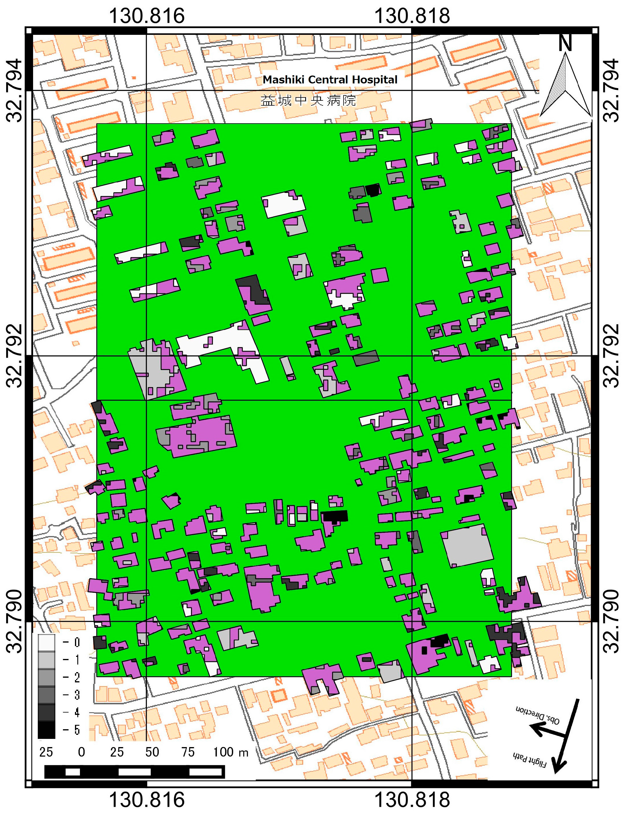
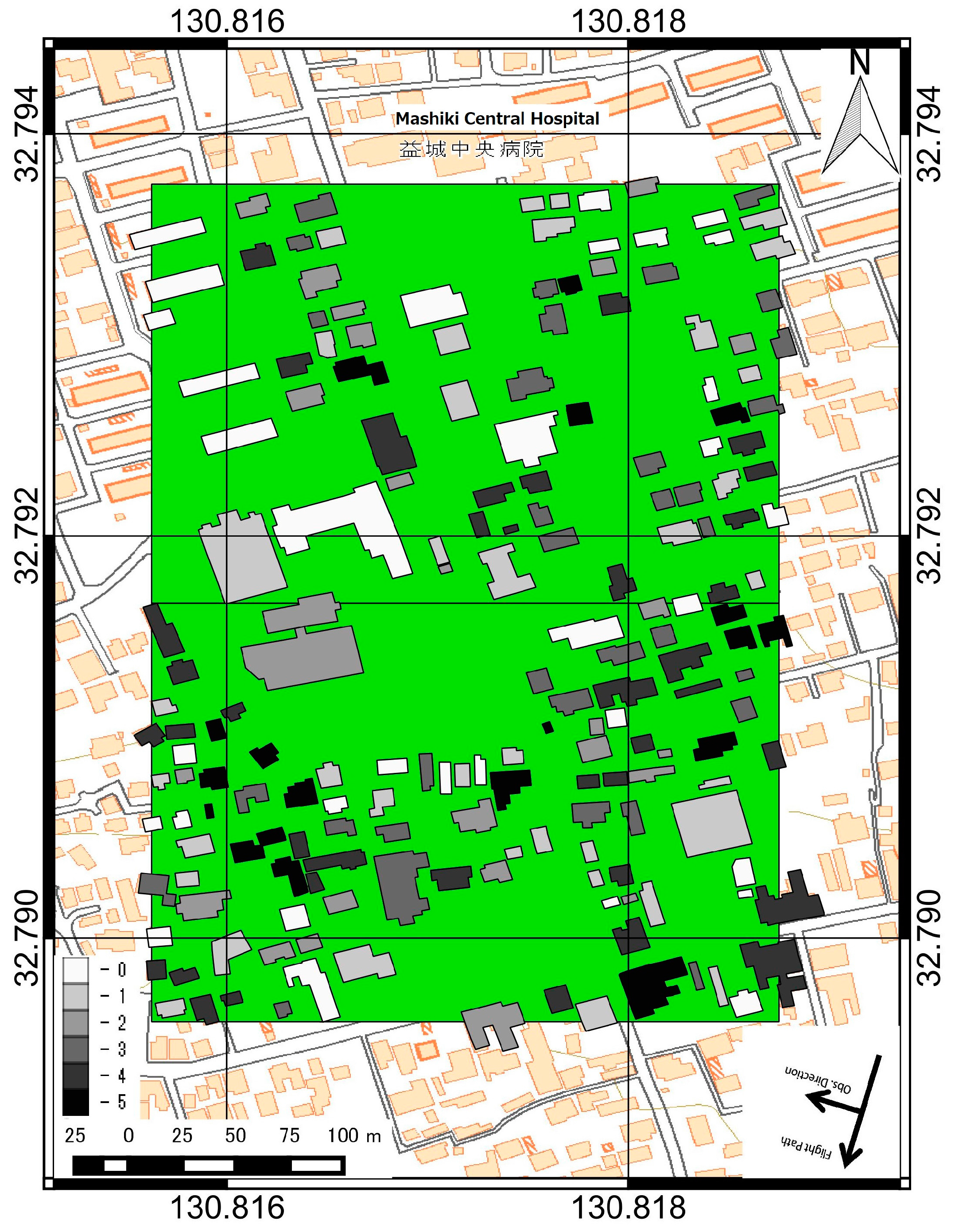
2.3. Inventory Survey Results in Sampled Region of Mashikimachi Town

The National Research Institute for Earth Science and Disaster Resilience (NIED) performed an inventory survey of 185 buildings in the 250 m × 500 m area of Mashikimachi town (B in Figure 1) [33]. They classified the damaged buildings by the structural types and damage patterns based on [34,35] that are compatible with the damage grade in EMS-98 [24]. The size of the buildings and their damage level (DL) are shown in Table 1. The distribution and the size of the buildings include a high enough number of samples. The actual distribution of the buildings is shown in Figure 3.
For example, DL 2 represents moderate damage (slight structural damage, moderate non-structural damage) of the buildings, while DL 5 represents a total collapse of the building, as can be seen in the EMS-98-based evaluation. That is, the buildings have significant damage on their surface when the DL is larger than 2.
We compare the coherence change detection results and the inventory survey with the following parameters in order to find the relationship between coherence decrease (CD) and DL:
  • Threshold of the coherence decrease (CD) un.
  • The smallest size of the building to judge.
  • Ratio of the CD region per building CDregion   size Overall   size .
“CD region size” represents the size of the area or the building for which the CD value is larger than the threshold. “Overall size” represents the size of the building. For example, if 50 m2 out of 200 m2 of the building shows a CD value that is larger than the threshold, the ratio of the CD region becomes 50/200 = 0.4. To obtain the best parameter to acquire the highest accuracy, we performed a full search among these three parameters and calculated the user’s and producer’s accuracy including Cohen’s Kappa coefficient.

3. 2016 Kumamoto, Japan Earthquakes and ALOS-2 Observations

Here, we briefly describe the 2016 Kumamoto, Japan Earthquakes. On 14 and 16 April 2016, three large earthquakes hit Kumamoto Prefecture, Japan, with moment magnitudes (Mw) of 6.2, 6.0, and 7.0, respectively [27]. Buildings in Kumamoto city and the neighboring Mashikimachi town incurred severe damage [25]. The main deformation occurred 40 km along the Futagawa and Hinagu faults from south-west to north-east [28].
As a duty of the disaster response mission, JAXA operated ALOS-2 to observe the affected area. ALOS-2 successfully observed almost all the affected area with 3-m resolution mode acquisitions. In this paper, we use the observation datasets from the Path 23 observed on 7 March and 18 April 2016 and 30 November 2015 for the interferometric coherence analysis. The temporal and perpendicular baselines are 98 days and 107 m for the 30 November 2015–7 March 2016 pair and 42 days and 126 m for the 7 March–18 April 2016 pair. Observations from other tracks were not used in this paper because there were no better pairs. Thus, the orientation of the building is not discussed in this paper.
A local and nonlinear co-registration [36] was performed for InSAR analysis in addition to traditional cross-correlation-based 2D polynomial co-registration in this paper. This process was done to overcome the decreased coherence. There are nonlinear pixel offsets in SAR images derived from tectonic movement caused by the earthquake. On the other hand, no multilooking and filtering were performed because the aim of this paper is not to evaluate the ground deformation, but to analyze the interferometric coherence.

4. Experimental Results

4.1. Aerial Photography Survey in a Larger Scale

In the study area around the Kumamoto urban district, a heterogeneous spatial distribution of coherence decrease (CD) is shown in Figure 4a. Higher CD values are mainly located closer to the main faults (i.e., southeastern corner of this figure), whereas some places denote a slightly high concentration of the higher CD.
In this rectangle, 165,177 buildings had been originally located, as shown in Figure 4b. Compared with the geomorphological classification map, major distributions of 40.2% buildings on terraces, 14.8% on alluvial fans, 15.0% on flood plains, and 8.0% on natural levees are found, whereas the rest of the geomorphic classification has less than 5% buildings (Table 2; Figure 4b and Figure 5a). In this area, 15,668 buildings (9.5%) covered with plastic sheets are identified, which are located with geospatial heterogeneity (Figure 4b). In the above-mentioned geomorphic conditions with major building distributions, 12.5% on terraces, 6.3% on natural levees, 5.2% on alluvial fans, and 5.1% on flood plains are covered with plastic sheets, whereas 7.9% of the buildings are sheet-covered in other classifications (Table 2; Figure 5b). The spatial distribution of CD that is shown in Figure 4a is summarized in Figure 5c, classified into the geomorphological groups. All the groups show a similar proportion of CD intensity with higher proportions for lower CD values (Figure 5c).
In terms of geological condition, major distributions of the original buildings are found at 35.1% on Late Pleistocene to Holocene marine and non-marine sediments, at 29.7% on the Late Pleistocene lower terrace, at 19.1% on the Late Pleistocene middle terrace, and at 13.7% on Late Pleistocene non-alkaline pyroclastic flow volcanic rocks, whereas the rest of the geomorphic classification has less than 3.0% buildings (Figure 5d). For these classified groups, 7.1%, 11.3%, 15.6%, and 15.8% of buildings are covered with plastic sheets, respectively (Figure 5e). The CD value distribution classified into the geological group does not denote a significant difference between the groups, which is also true for the geomorphological classification (Figure 5f).
Furthermore, the buildings are classified by the distance from the main faults. For the buildings located in “Terrace” and “Late Pleistocene to Holocene marine and non-marine sediments”, which form the majority of geomorphological classification and geological classification, respectively, the ratio of sheet-covered buildings and the mean CD value in each 100-m bin are profiled in Figure 6. A significant negative correlation is found at the CD value in “Terrace”, i.e., lower CD values for places located far away from the faults (Figure 6a). The sheet-covered ratio does not have a similar correlation, but has lower values at the places closest to the faults (<300 m) and higher values for the middle-range distance (300–600 m). In “Late Pleistocene to Holocene marine and non-marine sediments”, similar trends of the sheet-covered ratio and CD value are found, but are relatively more moderated compared to that for “Terrace”. As a result, we found that these optical and SAR observations reflect spatial distributions of buildings in different damage levels, respectively. The sensitivities of them are assessed in the following results.

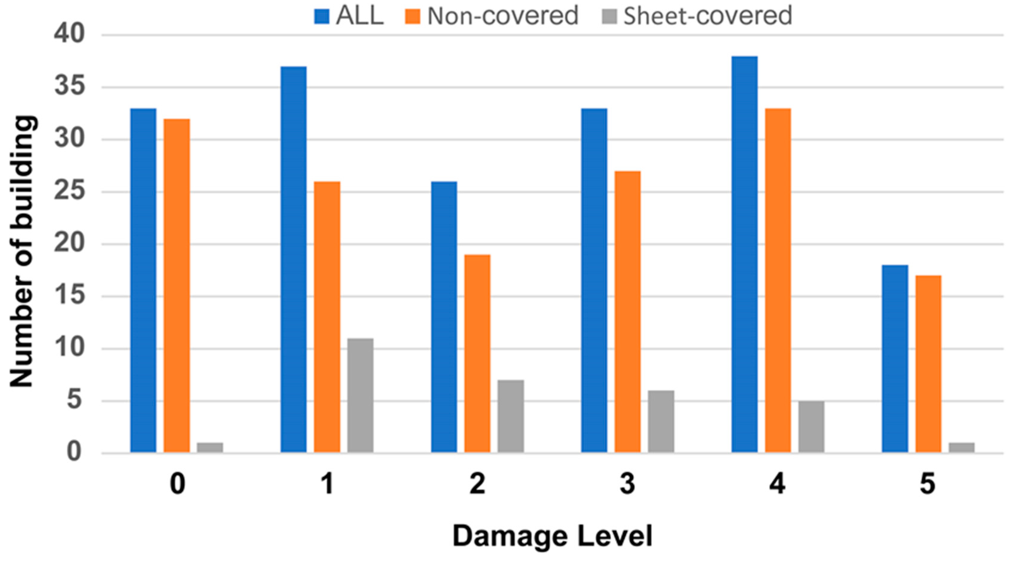
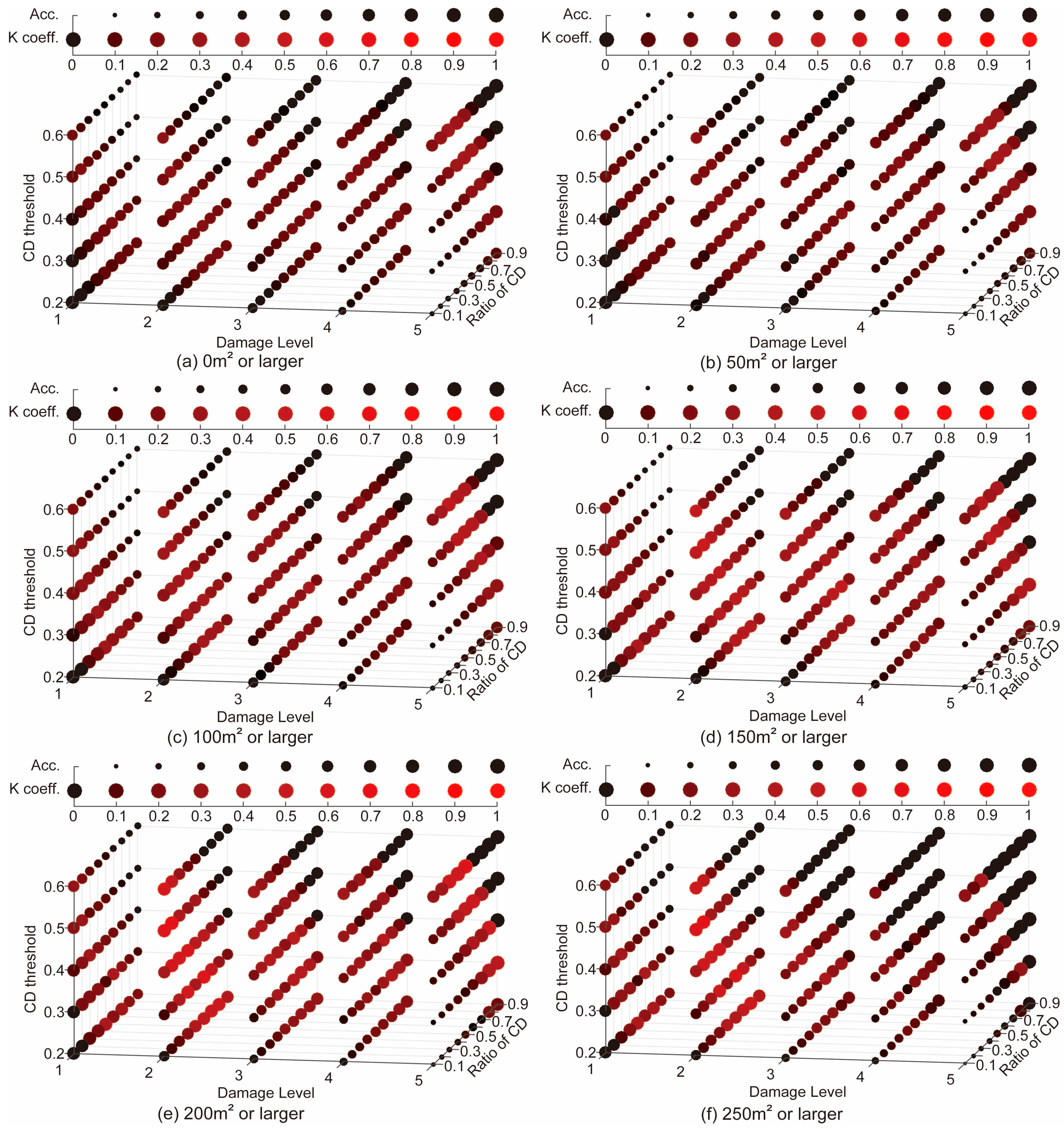
4.2. Inventory Survey in a Smaller Scale

We performed a full search among the three parameters shown in Section 2.3. The window size of the ensemble average for the coherence estimation is set to 5 × 5 pixels. We set the minimum size of the buildings for the evaluation from 0 m2 (all buildings) to 250 m2 (250 m2 or larger) at intervals of 50 m2. We set the threshold of un from 0.2 to 0.6 at 0.1 intervals and the ratio of the CD region per building from 0.1 to 0.9 at 0.1 intervals. Figure 7 presents the overall accuracy and the Cohen’s Kappa coefficient of the full search results. From Figure 7, the larger diameter of the circle represents a higher accuracy, while the brighter red circle represents a higher K coefficient, as shown in the upper column of the figures. If there is a large red circle, the CD threshold and Ratio of CD are set suitably to find the damaged buildings. As shown in Figure 7a–d, there are no reliable points. That is, it is not able to evaluate the damage level of the buildings smaller than 150 m2. On the other hand, Figure 7e has a relatively large red circle in the column of DL 2 and 5. In other words, if we set an appropriate threshold, we can detect the buildings that have DL 2 or higher and, with another threshold, we can detect DL 5 ones. Figure 7f has a large red circle in the column of DL 2, but no large circle in DL 5. In short, there is some correlation between interferometric coherence and DL 2–5 buildings whose size is larger than 200 m2. At the same time, there is no reliable threshold to detect DL 1, 3, or 4 in any building size. In summary, the buildings must satisfy two requirements to be categorized as “damaged”, as follows:
  • The size of the building is 200 m2 or larger.
  • The damage level of the building is DL 2 or higher.
If a building satisfies these requirements, the threshold and the ratio of the CD region per building show a correlation, as illustrated in Table 3.
Table 3 presents the overall accuracy and Cohen’s Kappa Coefficient for buildings larger than 200 m2 with DL 2 or higher. If we set the coherence threshold at 0.2, and set the ratio of the CD region per building from 0.5 to 0.8, the detection results show a high reliability. In other words, if 50–80% of the building is covered by a 0.2 or larger CD region, there is a high probability that the building’s DL is greater than 2. If we increase the coherence threshold to 0.3, for example, the ratio will be from 0.3 to 0.7 and a ratio of 0.6 marks the highest accuracy (82% and a Cohen’s Kappa coefficient of 0.63). The overall maximum score is marked when the coherence threshold is 0.5 and the ratio is 0.2, and in this situation, the accuracy and the Cohen’s Kappa coefficient were 0.84 and 0.68, respectively. The coverage of the region for which the coherence was decreased by more than 0.3 is shown in Figure 8 with the purple pixels. On the other hand, we could not find any reasonable score when we set the DL to 3 or 4. That is, there was no reasonable threshold which can distinguish between DL 3 or higher from 2 or lower, nor DL 4 or higher from 3 or lower. In the case of DL 5, we obtained some reliable results, as shown in Table 4. The maximum accuracy and Cohen’s Kappa coefficient were marked at the coherence threshold of 0.6 and the ratio of 0.5 and their scores were 0.95 and 0.64, respectively. Note that only four of 38 buildings have DL 5 and thus the result is not so reliable due to the low number of samples. If we set the coherence threshold to 0.3, the ratio of 0.9 marks the highest accuracy (89% and a Cohen’s Kappa coefficient of 0.44).
As a result, we found the following three facts:
  • If a building is too small, smaller than 200 m2 in this case, it is not possible to assess the DL with coherence analysis.
  • There were two thresholds. One is to detect DL 2 (moderate damaged) or higher (DL 3–5) buildings and, the other one is to detect DL 5 (totally collapsed) buildings. However, there was no appropriate threshold that can distinguish DL 3–5 or DL 4–5 from the others.
  • The threshold of the coherence has a proportional relationship with the ratio between CD region and the size of the building. Most damaged buildings present a little decrease of the coherence in the large part of the building, or a large decrease of the coherence in the small part of the building.
The physical mechanisms of these results are discussed in the following section.
Figure 9 presents the number of sheet-covered buildings in the same region. Eleven out of 37 DL 1 buildings and seven out of 26 DL 2 buildings were covered by sheets, while only 12 out of 89 DL 3–5 buildings were covered. This result indicates that sheet-covered buildings correspond to slightly or moderately damaged buildings in architectural assessments. This is the reason why there is no correlation between sheet-covered and high CD buildings in Section 4.1. SAR interferometric analysis can detect moderate or higher damaged buildings, while optical analysis can detect lower damages.

5. Discussion

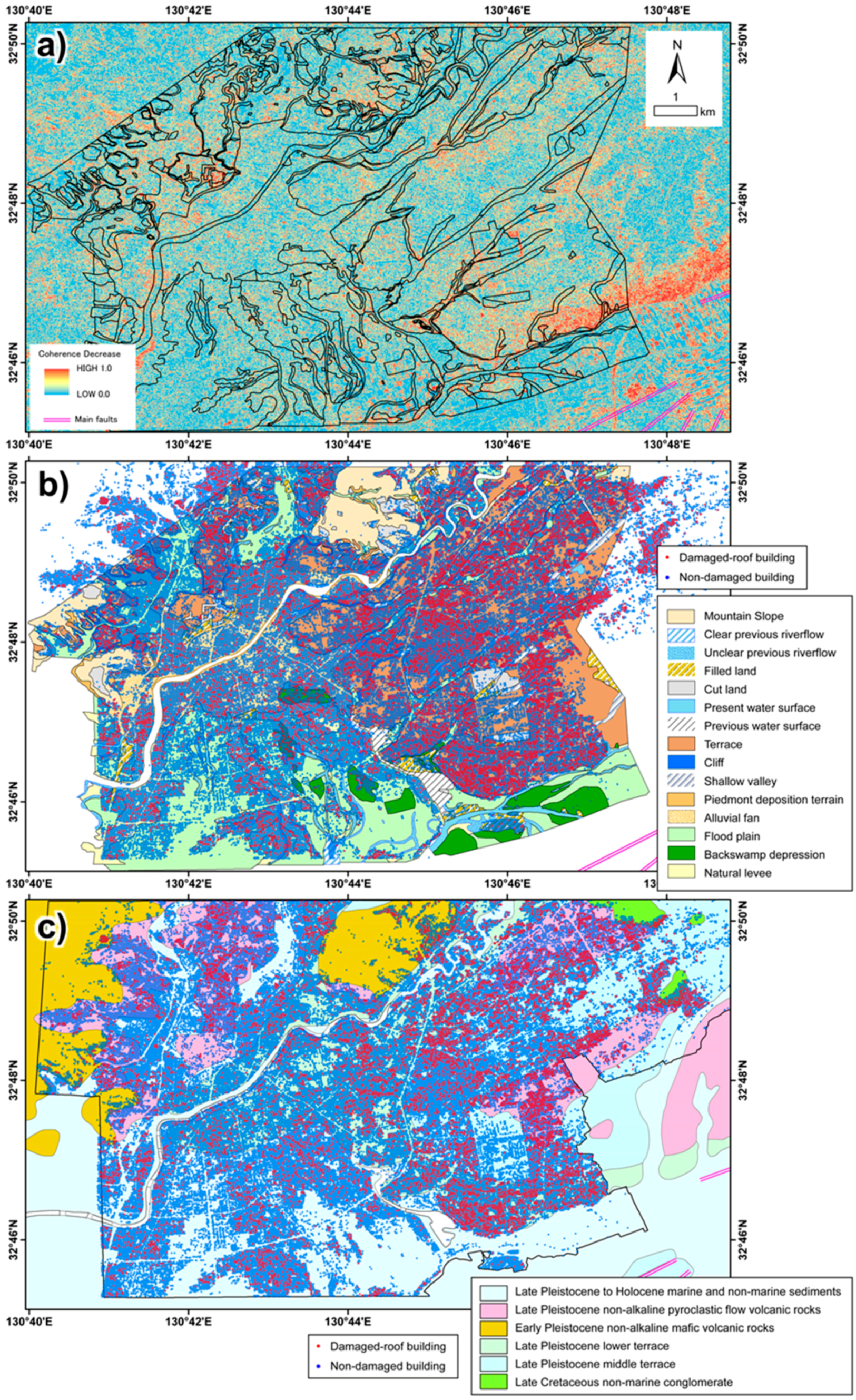
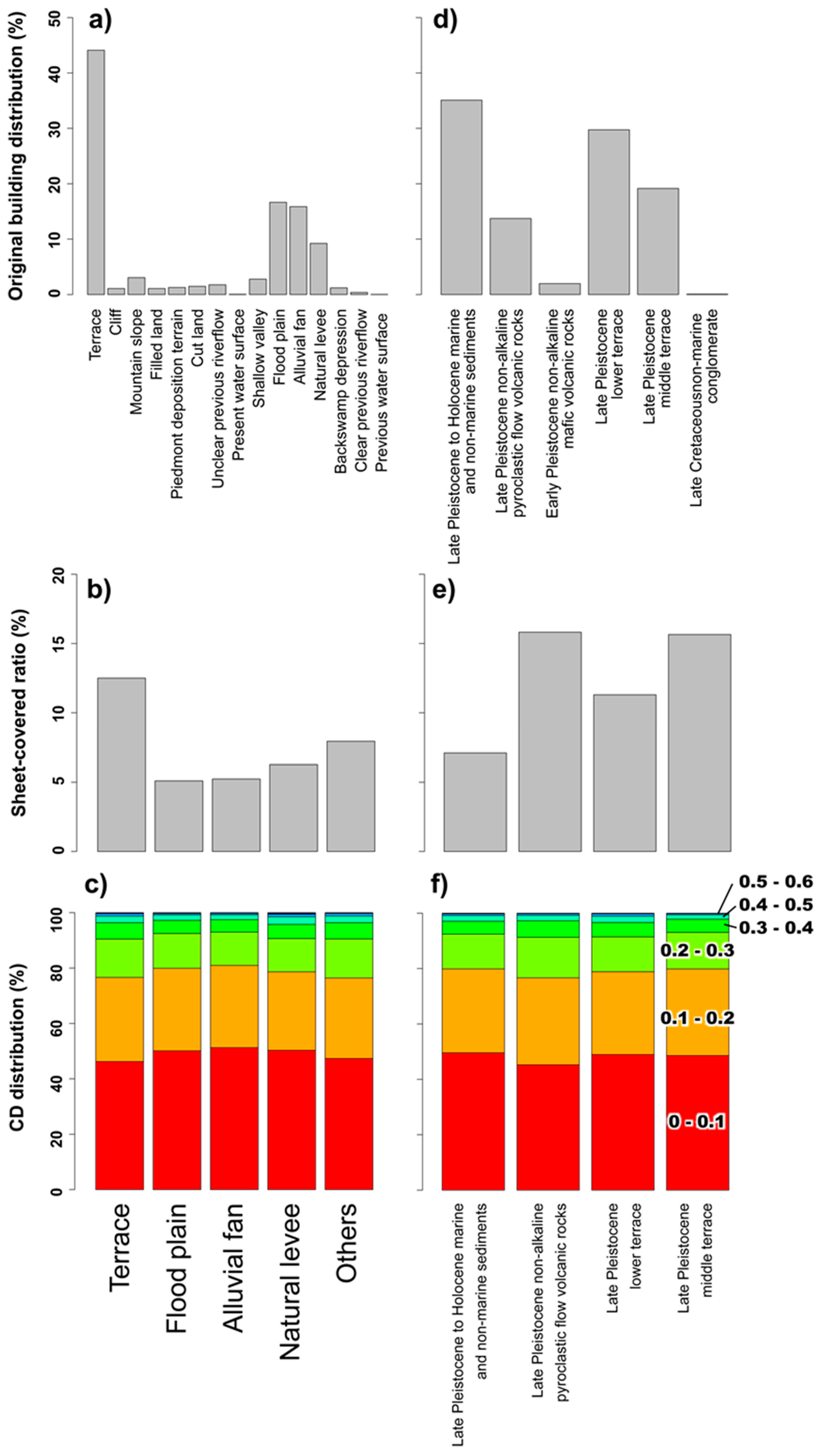
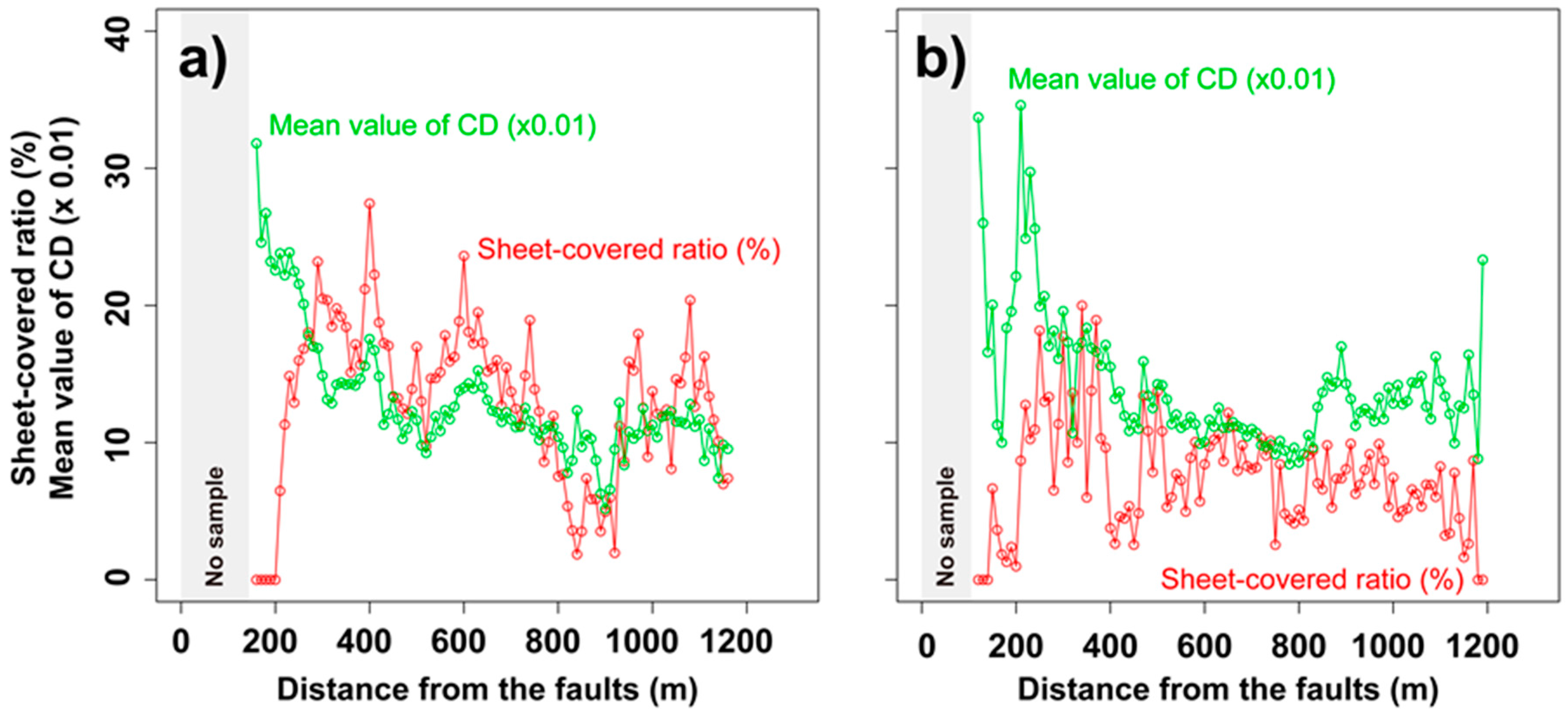
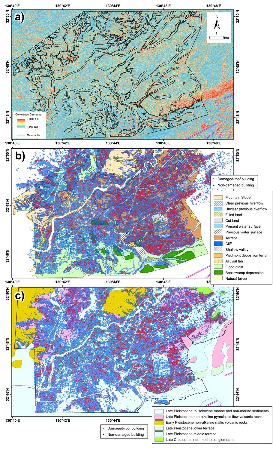
5.1. Distribution of Damaged Buildings

Individual DLs are assessed for buildings around the urban district of Kumamoto, extracting plastic sheets on the roof. The sheet-covered buildings are mostly located at geomorphologically-classified “Terrace” (Figure 4b) and geologically-classified “Late Pleistocene non-alkaline pyroclastic flow volcanic rocks”, as well as “Late Pleistocene lower terrace” (Figure 4e), followed by other groups. These classifications likely have harder and solider bedrocks for building construction than the others such as “Flood plain”, “Alluvial fan”, and “Natural levee”. Therefore, it can be considered that harder and solider bedrocks amplified the earthquake-induced shaking to the ground surface, when compared to other buildings located at the same distance from the faults. In terms of the distance from the faults, the closest places have a lower proportion of sheet-covered buildings (Figure 6a), which can be explained by the fact that severely-damaged buildings would not have been covered with sheets but abandoned. These considerations suggest that covering a building with a plastic sheet is a proxy for medium level damaged buildings, which is primarily related to geomorphological condition followed by the distance from the faults.
In contrast, CD is not influenced by geomorphological and geological classifications (Figure 5c,f), but significantly correlated with the distance from the main faults (Figure 6). It suggests that the CD distribution is briefly related to the ground deformation in addition to the spatial distribution of higher level damaged buildings. Geologically homogeneous conditions (“Late Pleistocene non-alkaline pyroclastic flow volcanic rocks”) (Figure 6b) have a more moderate correlation than geomorphologically homogeneous conditions (“Terrace”) (Figure 6a) in terms of the CD-and-distance correlation. This suggests a possibility that artificial and hydrological surface modification after bedrock exposure have considerable effects on the building damage level.

5.2. Ambiguity of Coherence Threshold

The CD in the non-damaged buildings is mainly caused by temporal decorrelation. Its treatment using the spatial coherence distribution was proposed, for example in [2,37,38]. However, according to the experimental results, the CD obtained from pre-and post-earthquake PALSAR-2 data denotes a statistically significant difference for damaged buildings. However, the mean values of the CD between the damaged buildings and the whole buildings (damaged + non-damaged) exhibit less difference; therefore, further improvement is required if this method is to be used for the actual application of damage detection of individual buildings.
From the experimental results of the inventory survey, the threshold itself is not a significant issue compared to the insufficient size of the building.

5.3. Minimum Size of the Buildingc

From the experimental results, it is not possible to distinguish DL 3 or 4 from the other levels. In addition, it is not possible to assess the DL with coherence analysis for buildings smaller than 200 m2. These results can be explained by the physical mechanism of the DL and the coherence analysis.
First, the CD is caused by the increase of the random displacement of the dominant scatterer. In DL 2 and higher cases, the buildings present significant damage on their surface. This is the reason why the coherence analysis can detect DL 2 or higher. On the other hand, an SAR cannot observe inside of the building and thus, the coherence analysis cannot evaluate the structural damage. If the building is totally collapsed, that is regarded as DL 5, the coherence decreases significantly, and it becomes able to be distinguished from the other DLs.
Next, the coherence value is calculated from averaging the specific number of pixels. In other words, the coherence value cannot be derived from a single pixel but inside the window surrounding the target pixel. There is a tradeoff in that a small window size will overestimate the coherence value, while a large window will reduce the spatial resolution. In this paper, we applied a 5 × 5 window following [39,40] and the ground resolution of the ALOS-2 was approximately 3 m. In summary, the coherence value is derived from the approximately 15 × 15 m window. Thus, the lowest size of the building that can be evaluated depends on the size of the window. Because a smaller window overestimates the coherence value, SAR resolution must be improved to evaluate smaller buildings.

5.4. Origin of Low Coherency

Coherence value decreases not only with the building’s damage, but also for various other reasons.
  • Temporal decorrelation
We ignored the temporal decorrelation in this paper because the pre-disaster pair has a longer temporal baseline (30 November 2015–7 March 2016) than the co-disaster pair (7 March 2016–18 April 2016). The 98-day temporal baseline of the pre-disaster pair is longer than the scheduled ALOS-2 observation cycle and thus, its interferometric coherence shows significant temporal decorrelation in vegetated areas. However, according to [16], interferometric coherence is high enough for a more than two-year temporal baseline. As we are interested in urban areas, we regard that the temporal decorrelation in urban areas is smaller than in vegetated areas and decided to ignore this component by modifying the threshold. Note that outside of the city, rice pads may have been filled by water in the co-disaster pair while they were dry in the winter. We regard that these agricultural and other environmental reasons do not affect the coherence in the urban area.
  • Baseline decorrelation
A long baseline between two observations causes a baseline decorrelation. However, ALOS-2 is controlled to achieve a small baseline. As a result, the pre-disaster pair and co-disaster pair had 107 m and 125 m perpendicular baselines, respectively. These baselines are short enough to ignore the baseline decorrelation.
  • Ionospheric and tropospheric decorrelations
In general, an L-band space-borne SAR interferogram contains ionospheric and tropospheric delay components which derive an additional decrease of the interferometric coherence. Analytical results show that these effects are negligible for the dataset used in this paper.
  • Decorrelation in phase discontinuities
In the Kumamoto earthquakes, multiple lineaments were found along and across the main faults [41]. These lineaments represent small faults, liquefactions, and landslides. The direction and amount of ground deformation differ from one side of the lineament to the other side, resulting in discontinuous phases in the interferometric phase in the InSAR analysis. In summary, the phase pattern is relatively inhomogeneous along the phase discontinuous region. Some low coherence regions suggest the existence of these lineaments. However, the distribution of the lineaments does not affect the distribution/density of the damaged buildings, but the main fault does in this case (see Section 5.1). A dense fringe pattern also derives low interferometric coherence [42]. The threshold of CD must consider this point. The area where the survey was performed in Section 4.2 was far enough from the lineaments and has a similar fringe density. Therefore, we ignored this effect in this paper. Further analysis is required to find the method to derive the best CD threshold in a general case.

6. Conclusions

In this paper, the sensitivity and the limitation of the SAR interferometric coherence for the damage detection of individual buildings are evaluated. The larger scale observations in the Kumamoto central district denote that severe damage is more dominant in places located closer to the quake-induced main faults, less affected by geomorphological and geological conditions. Medium damage is significantly affected by geomorphologically and geologically strong features rather than the distance from the faults. The experimental results at a smaller scale at severely-damaged sites show two aspects. First, there is a correlation between the buildings which can be distinguished as severely or medium damaged, and the buildings which interferometric coherence decreased by more than 0.3 in this case. Second, if the buildings are large (>200 m2), there is a strong correlation between the buildings for which interferometric coherence decreased by more than 0.3 and, buildings whose damage levels (DLs) were Level 2 or heavier when the damage level was classified by EMS-98. This case study suggests that interferometric coherence can be used for detecting the moderately damaged (DL 2 or heavier) buildings in addition to the severely damaged (DL 5) ones. However, the derived parameters are specified for 2016 Kumamoto Earthquakes. It is currently difficult to define the threshold values in a general case. Further researches are required.

Acknowledgments

This research is partially supported by the Council for Science, Technology, and Innovation (CSTI), “Cross-ministerial Strategic Innovation Promotion Program” (SIP), “Enhancement of societal resiliency against natural disasters” (Funding agency: JST). We thank Takuma Saeki (NIED) for providing the inventory survey data in Mashikimachi town. We also thank the Working Group for SAR Analysis, the Coordinating Committee for Earthquake Prediction Japan for their early response in the earthquakes. The Geospatial Information Authority under the Ministry of Land, Infrastructure, Transport and Tourism of Japan provided digitized building data and geomorphological maps for flood prevention. Google Inc. provided the three-dimensional view of pre-quake ground object models on Google Earth.

Author Contributions

R.N. and H.N. conceived, designed, and performed the experiments; R.N. performed the interferometric coherence analysis and compared it with an inventory survey; H.N. evaluated the InSAR results with an aerial photography survey; N.T. and T.T. managed this research.

Conflicts of Interest

The authors declare no conflict of interest.

References

  1. Plank, S. Rapid damage assessment by means of multi-temporal SAR—A comprehensive review and outlook to Sentinel-1. Remote Sens. 2014, 6, 4870–4906. [Google Scholar] [CrossRef] [Green Version]
  2. Milillo, P.; Riel, B.; Minchew, B.; Yun, S.H.; Simons, M.; Lundgren, P. On the synergistic use of SAR constellations’ data exploitation for earth science and natural hazard response. IEEE J. Sel. Top. Appl. Earth Observ. Remote Sens. 2016, 9, 1095–1100. [Google Scholar] [CrossRef]
  3. Stramondo, S.; Bignami, C.; Chini, M.; Pierdicca, N.; Tertulliani, A. Satellite radar and optical remote sensing for earthquake damage detection: Results from different case studies. Int. J. Remote Sens. 2006, 27, 4433–4447. [Google Scholar] [CrossRef]
  4. Brunner, D.; Lemoine, G.; Bruzzone, L. Earthquake damage assessment of buildings using VHR optical and SAR imagery. IEEE Trans. Geosci. Remote Sens. 2010, 48, 2403–2420. [Google Scholar] [CrossRef]
  5. Matsuoka, M.; Yamazaki, F. Building damage mapping of the 2003 Bam, Iran, earthquake using ENVISAT/ASAR intensity imagery. Earthq. Spectra 2005, 21, S285–S294. [Google Scholar] [CrossRef]
  6. Fielding, E.J. Surface ruptures and building damage of the 2003 Bam, Iran, earthquake mapped by satellite synthetic aperture radar interferometric correlation. J. Geophys. Res. 2005, 110. [Google Scholar] [CrossRef] [Green Version]
  7. Arciniegas, G.A.; Bijker, W.; Kerle, N.; Tolpekin, V.A. Coherence- and amplitude-based analysis of seismogenic damage in bam, Iran, using ENVISAT ASAR data. IEEE Trans. Geosci. Remote Sens. 2007, 45, 1571–1581. [Google Scholar] [CrossRef]
  8. Yamaguchi, Y. Disaster monitoring by fully polarimetric SAR data acquired with ALOS-PALSAR. Proc. IEEE 2012, 100, 2851–2860. [Google Scholar] [CrossRef]
  9. Sato, M.; Chen, S.W.; Satake, M. Polarimetric SAR analysis of tsunami damage following the March 11, 2011 East Japan Earthquake. Proc. IEEE 2012, 100, 2861–2875. [Google Scholar] [CrossRef]
  10. Watanabe, M.; Motohka, T.; Miyagi, Y.; Yonezawa, C.; Shimada, M. Analysis of urban areas affected by the 2011 off the pacific coast of Tohoku Earthquake and Tsunami with L-band SAR full-polarimetric mode. IEEE Geosci. Remote Sens. Lett. 2012, 9, 472–476. [Google Scholar] [CrossRef]
  11. Chen, S.W.; Sato, M. Tsunami damage investigation of built-up areas using multitemporal spaceborne full polarimetric SAR images. IEEE Trans. Geosci. Remote Sens. 2013, 51, 1985–1997. [Google Scholar] [CrossRef]
  12. Chen, S.W.; Wang, X.S.; Sato, M. Urban damage level mapping based on scattering mechanism investigation using fully polarimetric SAR data for the 3.11 East Japan earthquake. IEEE Trans. Geosci. Remote Sens. 2016, 54, 6919–6929. [Google Scholar] [CrossRef]
  13. Nakmuenwai, P.; Yamazaki, F.; Liu, W. Multi-temporal correlation method for damage assessment of buildings from high-resolution SAR images of the 2013 typhoon Haiyan. J. Disaster Res. 2016, 11, 577–592. [Google Scholar] [CrossRef]
  14. Bouaraba, A.; Younsi, A.; Belhadj-Aissa, A.; Acheroy, M.; Milisavljevic, N.; Closson, D. Robust techniques for coherent change detection using COSMO-SkyMed SAR images. Prog. Electromagn. Res. M 2012, 22, 219–232. [Google Scholar] [CrossRef]
  15. Chini, M.; Albano, M.; Saroli, M.; Pulvirenti, L.; Moro, M.; Bignami, C.; Falcucci, E.; Gori, S.; Modoni, G.; Pierdicca, N.; et al. Coseismic liquefaction phenomenon analysis by COSMO-SkyMed: 2012 Emilia (Italy) earthquake. Int. J. Appl. Earth Observ. Geoinf. 2015, 39, 65–78. [Google Scholar] [CrossRef]
  16. Wei, M.; Sandwell, D.T. Decorrelation of L-band and C-band interferometry over vegetated areas in California. IEEE Trans. Geosci. Remote Sens. 2010, 48, 2942–2952. [Google Scholar]
  17. Yonezawa, C.; Takeuchi, S. Decorrelation of SAR data by urban damages caused by the 1995 Hyogokennanbu earthquake. Int. J. Remote Sens. 2011, 22, 1585–1600. [Google Scholar] [CrossRef]
  18. Matsuoka, M.; Nojima, N. Building damage estimation by integration of seismic intensity information and satellite L-band SAR imagery. Remote Sens. 2010, 2, 2111–2126. [Google Scholar] [CrossRef]
  19. Gokon, H.; Koshimura, S.; Meguro, K. Verification of a method for estimating building damage in extensive tsunami affected areas using L-band SAR data. J. Disaster Res. 2017, 12, 251–258. [Google Scholar] [CrossRef]
  20. Arikawa, Y.; Saruwatari, H.; Hatooka, Y.; Suzuki, S. PALSAR-2 launch and early orbit operation result. In Proceedings of the 2014 IEEE International Geoscience and Remote Sensing Symposium (IGARSS), Quebec City, QC, Canada, 13–18 July 2014; pp. 3406–3409. [Google Scholar]
  21. Bai, Y.; Adriano, B.; Mas, E.; Gokon, H.; Koshimura, S. Object-based building damage assessment methodology using only post event ALOS-2/PALSAR-2 dual polarimetric SAR intensity images. J. Disaster Res. 2017, 12, 259–271. [Google Scholar] [CrossRef]
  22. Watanabe, M.; Thapa, R.B.; Ohsumi, T.; Fujiwara, H.; Yonezawa, C.; Tomii, N.; Suzuki, S. Detection of damaged urban areas using interferometric SAR coherence change with PALSAR-2. Earth Planets Space 2016, 68. [Google Scholar] [CrossRef]
  23. Dell Acqua, F.; Gamba, P. Remote sensing and earthquake damage assessment: Experiences, limits, and perspectives. Proc. IEEE 2012, 100, 2876–2890. [Google Scholar] [CrossRef]
  24. Grunthal, G. (Ed.) European Macroseismic Scale 1998; Centre Europeen de Geodynamique et de Seismologie: Luxembourg, 1998. [Google Scholar]
  25. Liu, W.; Yamazaki, F. Extraction of collapsed buildings in the 2016 Kumamoto earthquake using multitemporal PALSAR-2 data. J. Disaster Res. 2017, 12, 241–250. [Google Scholar] [CrossRef]
  26. Natsuaki, R.; Anahara, T.; Kotoura, T.; Iwatsuka, Y.; Tomii, N.; Katayama, H.; Nishihata, T. Synthetic aperture radar interferometry for disaster monitoring of harbor facilities. J. Disaster Res. 2017, 12, 526–535. [Google Scholar] [CrossRef]
  27. Yoshida, K.; Hasegawa, A.; Saito, T.; Asano, Y.; Tanaka, S.; Sawazaki, K.; Urata, Y.; Fukuyama, E. Stress rotations due to the M 6.5 foreshock and M 7.3 main shock in the 2016 Kumamoto, SW Japan, earthquake sequence. Geophys. Res. Lett. 2016, 43, 10097–10104. [Google Scholar] [CrossRef]
  28. Uchide, T.; Horikawa, H.; Nakai, M.; Matsushita, R.; Shigematsu, N.; Ando, R.; Imanishi, K. The 2016 Kumamoto–Oita earthquake sequence: Aftershock seismicity gap and dynamic triggering in volcanic areas. Earth Planets Space 2016, 68. [Google Scholar] [CrossRef]
  29. Google, New 3D Imagery for Google Earth. Available online: https://www.youtube.com/watch?v=N6Douyfa7l8 (accessed on 17 April 2017).
  30. Geospatial Information Authority (GSI) of Japan, Vector-Format Feature Data. Available online: http://www.gsi.go.jp/kiban/ (accessed on 17 April 2017). (In Japanese)
  31. Geological Survey of Japan, AIST (Ed.) Seamless digital geological map of Japan 1: 200000. 8 December 2017 version. Geological Survey of Japan, National Institute of Advanced Industrial Science and Technology. 2017. Available online: https://gbank.gsj.jp/seamless/index_en.html (accessed on 13 January 2017).
  32. Geospatial Information Authority (GSI) of Japan, Geomorphic Classification Map for Flood Control. Available online: http://www.gsi.go.jp/bousaichiri/fc list a.html (accessed on 17 April 2017). (In Japanese).
  33. Saeki, T. Building damage survey of 2016 Kumamoto earthquake. In Proceedings of the Sixth Workshop of Japan-New Zealand-Taiwan Seismic Hazard Assessment 2016, Beppu, Japan, 31 October–4 November 2016. [Google Scholar]
  34. Okada, S.; Takai, N. Classifications of structural types and damage patterns of buildings for earthquake field investigation. J. Struct. Constr. Eng.-AIJ 1999, 524, 65–72. (In Japanese) [Google Scholar] [CrossRef]
  35. Takai, N.; Okada, S. Classifications of damage patterns of reinforced concrete buildings for earthquake field investigation. J. Struct. Constr. Eng.-AIJ 2001, 549, 67–74. (In Japanese) [Google Scholar] [CrossRef]
  36. Natsuaki, R.; Hirose, A. InSAR local co-registration method assisted by shape-from-shading. IEEE J. Sel. Top. Appl. Earth Observ. Remote Sens. 2013, 6, 953–959. [Google Scholar] [CrossRef]
  37. Yun, S.; Fielding, E.; Webb, F.; Simons, M. Damage Proxy Map from InSAR Coherence. U.S. Patent Application Serial Number: 13/528,610, 22 June 2012. [Google Scholar]
  38. Yun, S.H.; Hudnut, K.; Owen, S.; Webb, F.; Simons, M.; Sacco, P.; Gurrola, E.; Manipon, G.; Liang, C.; Fielding, E.; et al. Rapid Damage Mapping for the 2015 Mw 7.8 Gorkha Earthquake Using Synthetic Aperture Radar Data from COSMO–SkyMed and ALOS-2 Satellites. Seismol. Res. Lett. 2015, 86, 1549–1556. [Google Scholar] [CrossRef]
  39. Touzi, R.; Lopes, A.; Bruniquel, J.; Vachon, P.W. Coherence estimation for SAR imagery. IEEE Trans. Geosci. Remote Sens. 1999, 37, 135–149. [Google Scholar] [CrossRef]
  40. Lopez-Martinez, C.; Pottier, E. Coherence estimation in synthetic aperture radar data based on speckle noise modeling. Appl. Opt. 2007, 46, 544–558. [Google Scholar] [CrossRef] [PubMed]
  41. Fujiwara, S.; Yarai, H.; Kobayashi, T.; Morishita, Y.; Nakano, T.; Miyahara, B.; Nakai, H.; Miura, Y.; Ueshiba, H.; Kakiage, Y.; et al. Small-displacement linear surface ruptures of the 2016 Kumamoto earthquake sequence detected by ALOS-2 SAR interferometry. Earth Planets Space 2016, 68. [Google Scholar] [CrossRef]
  42. Zebker, H.A.; Chen, K. Accurate estimation of correlation in InSAR observations. IEEE Geosci. Remote Sens. Lett. 2005, 2, 124–127. [Google Scholar] [CrossRef]
Figure 1. Study areas in the central Kumamoto, Japan city. An aerial photography survey is carried out in (A) a Kumamoto central area and an inventory survey is carried out in (B) Mashikimachi near the main faults for this earthquake.
Remotesensing 10 00245 g001
Figure 2. Situations of post-earthquake Kumamoto city. (a) Damaged buildings are covered with plastic sheets, whereas (b) catastrophic and (c) older buildings are neglected. (d) Roofs covered with plastic sheets are identifiable from an airplane and (e) in Google Earth 3D models. (p) Other external materials and (q) lined walls are also covered with the sheet.
Remotesensing 10 00245 g002
Figure 3. Distribution of the damaged buildings in a sampled region of Mashikimachi town.
Remotesensing 10 00245 g003
Figure 4. Spatial distributions of (a) coherence decrease, buildings covered/non-covered with plastic sheets overlaid (b) on the geomorphological classification map and (c) on the geological map. The locations of these panels are the equivalent of (A) in Figure 1.
Remotesensing 10 00245 g004
Figure 5. (a) Original distributions of entire buildings, (b) sheet-covered ratios, and (c) numerical ratios of coherence decrease (CD) for whole buildings in each geomorphological classification shown in Figure 4c. Those classified into each geological classification (Figure 4b) are shown in (df), respectively. Several classification groups with few buildings are omitted in (b,c,e,f).
Remotesensing 10 00245 g005
Figure 6. Variations of sheet-covered ratio and mean value of CD corresponding to the distance from the main faults are summarized for (a) the geomorphological majority of “Terrace” and (b) the geological majority of “Late Pleistocene to Holocene marine and non-marine sediments”.
Remotesensing 10 00245 g006
Figure 7. Full search results for the overall accuracy and Cohen’s Kappa coefficient among multiple DLs (right to left), CD threshold (up to down), and ratio of CD (forward to backward). (af) Building threshold of 0 m2–250 m2 with 50 m2 intervals. The larger dot indicates the higher accuracy and the brighter red dot shows the higher K coefficient.
Remotesensing 10 00245 g007
Figure 8. Damage detection results for a coherence threshold of 0.3 in the sampled region of Mashikimachi town. Overlapped on Figure 3. Purple colored regions represent the pixels for which the CD values are larger than 0.3.
Remotesensing 10 00245 g008
Figure 9. Numbers of all, sheet-covered, and non-covered buildings in each damage level in the buildings inventoried in Mashikimachi.
Remotesensing 10 00245 g009
Table 1. Size and damage level (DL) of the buildings.
 DL012345Total
Size[m2] 
0–4921311210
50–9910144812250
100–149107111511660
150–19926276427
200–2490310228
≥25096526230
Total333726333818
Table 2. Summary of entire buildings and damaged-roof buildings.
Geomorphic TypeWhole BuildingDamaged Roof Building
Count(%)Count(%)
Mountain Slope46212.84379.5
Terrace66,38440.2864513.0
Cliff16901.01468.6
Shallow valley41822.557213.7
Piedmont deposition terrain18691.11508.0
Alluvial fan24,38914.813435.4
Floo plain24,79615.013125.3
Backswamp & depression17791.1965.4
Natural levee13,2238.08886.7
Clear previous riverflow5130.3193.7
Unclear previous riverflow23481.41466.2
Filled land16141.0483.0
Cut land22971.41285.6
Out of map15,4729.4173811.2
Sum165,177 15,668
Table 3. Overall accuracy and Cohen’s Kappa coefficient for coherence analysis with buildings over 200 m2 and with DL 2 or greater. Bold numbers with gray background represent the cells which accuracy and K-coefficient are over 0.7 and 0.4 respectively.
Overall Acc.Ratio of CD Region per Building
0.10.20.30.40.50.60.70.80.9
Coherence threshold0.20.530.550.580.630.710.740.760.760.68
0.30.550.630.710.790.680.820.740.630.58
0.40.680.790.790.790.710.710.630.550.47
0.50.820.840.680.630.660.550.500.470.47
0.60.790.740.630.550.530.470.470.470.47
K. Coeff.Ratio of CD Region per Building
0.10.20.30.40.50.60.70.80.9
Coherence threshold0.20.000.060.120.230.400.460.520.530.38
0.30.060.230.400.570.360.630.480.280.19
0.40.340.570.570.580.430.440.290.140.00
0.50.630.680.380.280.340.140.050.000.00
0.60.580.490.290.140.100.000.000.000.00
Table 4. Overall accuracy and Cohen’s Kappa coefficient for coherence analysis with buildings over 200 m2 and with DL 5 or greater. Bold numbers with gray background represent the cells which accuracy and K-coefficient are over 0.7 and 0.4 respectively.
Overall Acc.Ratio of CD Region per Building
0.10.20.30.40.50.60.70.80.9
Coherence threshold0.20.110.130.160.210.290.320.340.660.74
0.30.130.210.290.370.420.550.740.840.89
0.40.260.370.470.580.710.820.840.920.89
0.50.450.580.680.840.870.920.920.890.89
0.60.680.790.890.920.950.890.890.890.89
K Coeff.Ratio of CD Region per Building
0.10.20.30.40.50.60.70.80.9
Coherence threshold0.20.000.010.010.030.050.000.010.180.16
0.30.010.030.050.080.040.110.260.420.44
0.40.040.080.130.120.230.370.310.530.00
0.50.120.190.200.420.480.530.370.000.00
0.60.280.330.540.530.640.000.000.000.00

