An Observational Perspective of Sea Surface Salinity in the Southwestern Indian Ocean and Its Role in the South Asia Summer Monsoon


Faculty of Geo-Information Science and Earth Observation (ITC), University of Twente, Hengelosestraat 99, 7514 AE Enschede, The Netherlands
*
Author to whom correspondence should be addressed.
Remote Sens. 2018, 10(12), 1930; https://doi.org/10.3390/rs10121930
Submission received: 31 October 2018
/
Revised: 17 November 2018
/
Accepted: 27 November 2018
/
Published: 1 December 2018
(This article belongs to the Special Issue Sea Surface Salinity Remote Sensing)
Abstract
:The seasonal variability of sea surface salinity anomalies (SSSAs) in the Indian Ocean is investigated for its role in the South Asian Summer Monsoon. We have observed an elongated spatial-feature of the positive SSSAs in the southwestern Indian Ocean before the onset of the South Asian Summer Monsoon (SASM) by using both the Aquarius satellite and the Argo float datasets. The maximum variable areas of SSSAs in the Indian Ocean are along (60E–80E) and symmetrical to the equator, divided into the southern and northern parts. Further, we have found that the annual variability of SSSAs changes earlier than that of sea surface temperature anomalies (SSTAs) in the corresponding areas, due to the change of wind stress and freshwater flux. The change of barrier layer thickness (BLT) anomalies is in phase with that of SSSAs in the southwestern Indian Ocean, which helps to sustain the warming water by prohibiting upwelling. Due to the time delay of SSSAs change between the northern and southern parts, SSSAs, therefore, take part in the seasonal process of the SASM via promoting the SSTAs gradient for the cross-equator currents.
1. Introduction
The South Asian Summer Monsoon (SASM) forms a vital source of water for one-sixth of the world’s population. The onset and the intensity of the SASM control the occurrence of drought and flood events in South Asia, impacting on agricultural yields, water resources, infrastructure and humans. According to the monsoon’s dynamic theory, the northward shift of the intertropical convergence zone (ITCZ) marks the onset of the SASM whereby the dynamic aspects of the ocean play critical roles in modulating the strength of the monsoon [1]. It has been found that Sea Surface Temperature (SST) Anomalies (SSTAs) over the Indian Ocean are good indicators of the differential heating between ocean and land and are correlated with both the onset and the intensity of the SASM [2,3,4].
As water density is controlled by both temperature and salinity, evidence suggests that Sea Surface Salinity (SSS) could be an indicator of abrupt changes in ocean dynamic and air-sea interaction [5]. Salinity affects many aspects of ocean stability [6,7], dynamic ocean variability [8,9,10,11,12] and complicates air-sea interactions [13,14,15,16,17]. In previous studies [6,18], the variability of SSS is attributed to a series of complex mechanisms, mainly including the freshwater flux, horizontal advection, vertical entrainment as well as some turbulence of mixing and diffusion but the latter in the mixed layer has little influence on the seasonal variability of salinity [19,20,21].
Sea Surface Salinity Anomalies (SSSAs) have noticeable changes during SASM. For example, during the SASM season, the extent of SSSAs in the Indian mini warm pool region [22] is minimized and the freshwater belt is formed along the west coast of India [23]. SSS along the equatorial Indian Ocean can also reflect the imprints of Indian winter and summer monsoons via freshwater input and wind-induced mixing [24]. In 2004, minimum SSS was found before the onset of the monsoon [6]. Many scientific studies have shown that the inter-annual variability of SSSAs is connected to the local vortex of the monsoon onset [6,22,25,26] through the Arabian Sea mini warm pool.
Although the annual variance in SSS has been analysed in many studies [27,28,29], the annual variance in SSSAs is yet to be analysed. Neema et al. [22] revealed that the SSSAs in the Arabica Sea signal the onset of SASM by using only one-year simulated data, in this paper, we attempt to study the relationship between SSSA and SASM by providing observational and statistical evidence.
2. Data and Methods
SSS dataset. The SSS datasets comprised satellite products as well as in situ data. Satellite SSS products were obtained from the Version 5 Aquarius Combined Active-Passive (CAP) archive [30] for the period (09/2011–06/2015) on a grid of 0.5° × 0.5° (https://aquarius.umaine.edu/cgi/data_v5.htm). In situ measurements of SSS were obtained from the IPRC Array for Real-Time Geotropic Oceanography (Argo) product archive for the period (01/2005–12/2014) (http://apdrc.soest.hawaii.edu/projects/Argo).
Using in situ data obtained from Argo to study the Indian Ocean hold credibility because of the high density of data in the central Arabian Sea and central Bay of Bengal [31]. The Aquarius data, though limited in the period of coverage, are used for their higher spatial resolution to correct for discrepancies resulting from spatial interpolation of Argo data [32,33]. Both SSS data are mapped on a 1° × 1° grid on a monthly timescale.
Ancillary Datasets. The freshwater flux [Evaporation minus Precipitation (E-P)] is calculated using the monthly evaporation dataset obtained from the objectively analysed air-sea fluxes project (OAFLUX) [34] and monthly precipitation datasets from the Climate Prediction Centre (CPC) Merged Analysis of Precipitation (CMAP). Monthly MLD is also derived from Argo product provided by French Research Institute for Exploration of the Sea (Ifremer: http://www.ifremer.fr), with the MLD defined as the depth where the density has 0.03 kg/m3 difference from that of the surface [35].
Monthly SST dataset is used from NOAA Optimum Interpolation (OI) version 2 [36]. The atmospheric circulation is obtained from the monthly wind of ERA-Interim reanalysis data produced by the European Centre for Medium-Range Weather Forecasts (ECMWF) at standard pressure levels (1000 hPa − 100 hPa). Monthly barrier layer thickness (BLT) is calculated from Argo products provided by Ifremer, by the equation , where is the isothermal depth defined as the depth at which the surface temperature cools by 0.2 C and is the mixed layer depth [37,38].
All data used in this study are re-gridded into a 1° × 1° grid resolution from 2005 to 2014, except for wind stress which is from 2008 to 2014. The anomalies are calculated by the differences between the monthly data and climatological mean and the tendency of SSSAs and SSTAs are estimated by adopting the finite-difference method.
3. Observed Seasonal Variability in Sea Surface Salinity Anomalies
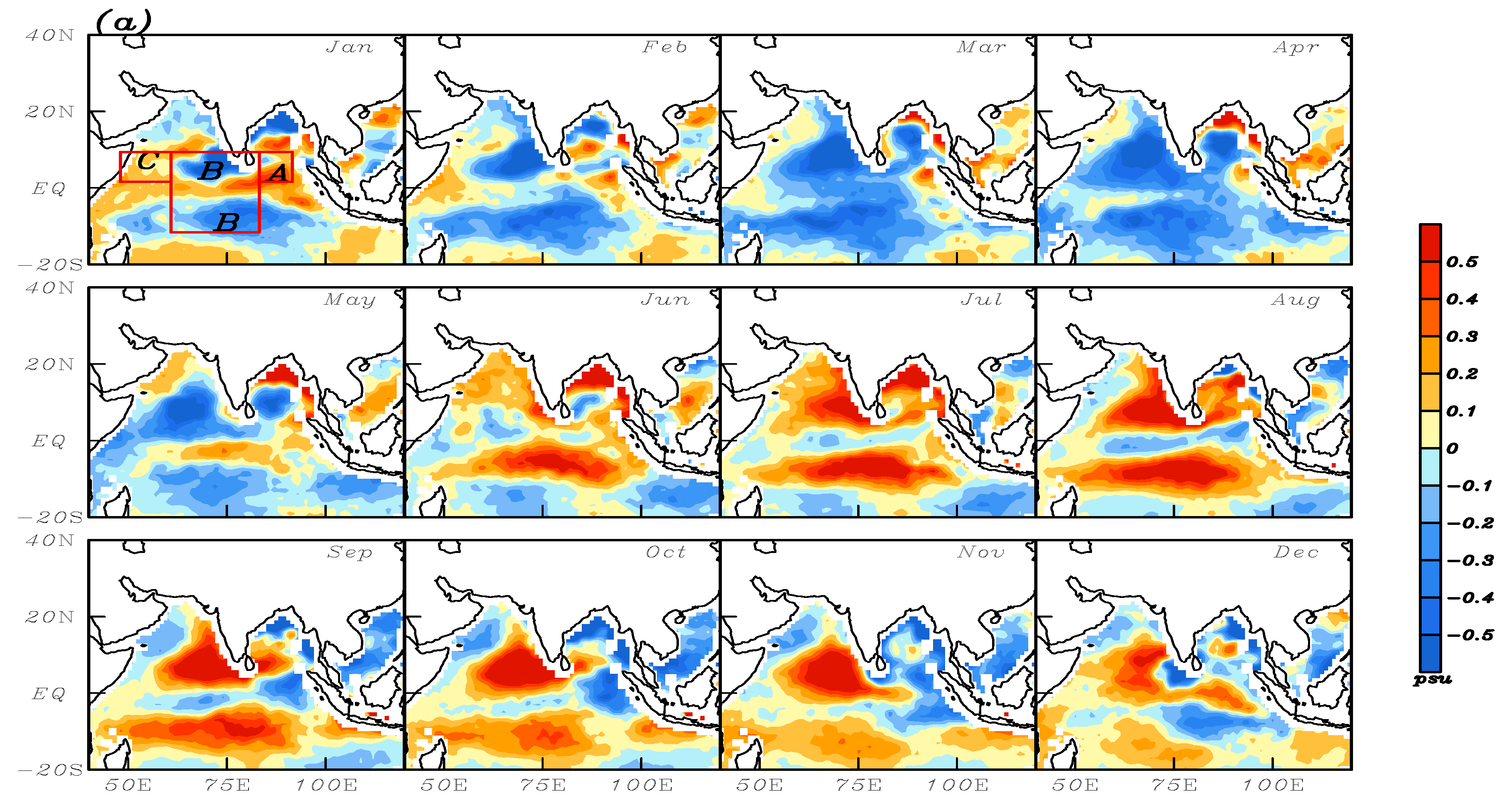
The SSS difference between the Arabian Sea and the Bay of Bengal, which is significant in climatological SSS distribution [28], was not found in monthly SSSAs. However, changes are apparent in several SSSAs maxima and minima centres shown by the Aquarius data (Figure 1a). For instance, in January, a positive SSSA centre appears in the eastern part (AEIO), a negative SSSA centre in the central part (BCIO) and a positive SSSA centre in the western part (CWIO), depicted in Figure 1a, respectively. From boreal winter to spring, the BCIO continuously intensifies and expands its area, whereas both the AEIO and CWIO diminish and disappear. In April, negative SSSAs distribute over almost the whole Indian Ocean. A notable change can be seen in May, with positive SSSAs slightly to the south of the equator, which may represent the suddenly intensifying AEIO. This positive SSSA, emerging as an elongated spatial feature (ESF), divides BCIO into two separated regions. Later, the positive SSSA ESF dominates almost the whole equatorial Indian Ocean and connects up with the intensifying CWIO in the northern Indian Ocean. Subsequently, the BCIO disappears during the boreal summer monsoon period with the positive SSSAs controlling the whole Indian Ocean, except for the equator and the western coast of the Arabian Sea. In the autumn, the positive SSSAs begin to dissipate gradually and the boreal winter mode is restored in December. This annual cycle of SSSAs also emerges when employing long-term SSS data obtained from Argo data for the period 2005–2014 (Figure 1b). Sparse subsampling of Argo data can reproduce the main features of the annual cycle defined by the satellite SSS from Aquarius.
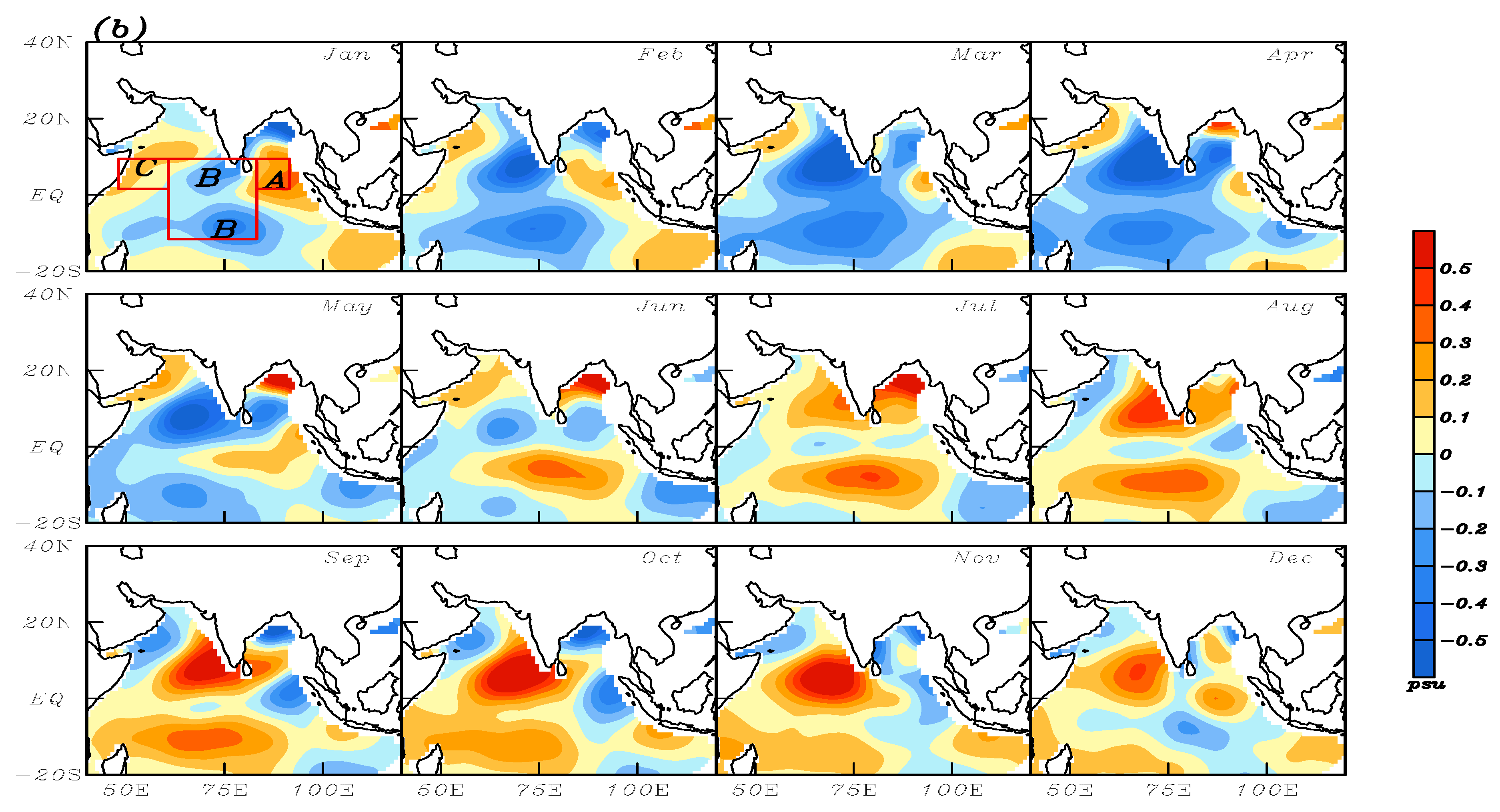
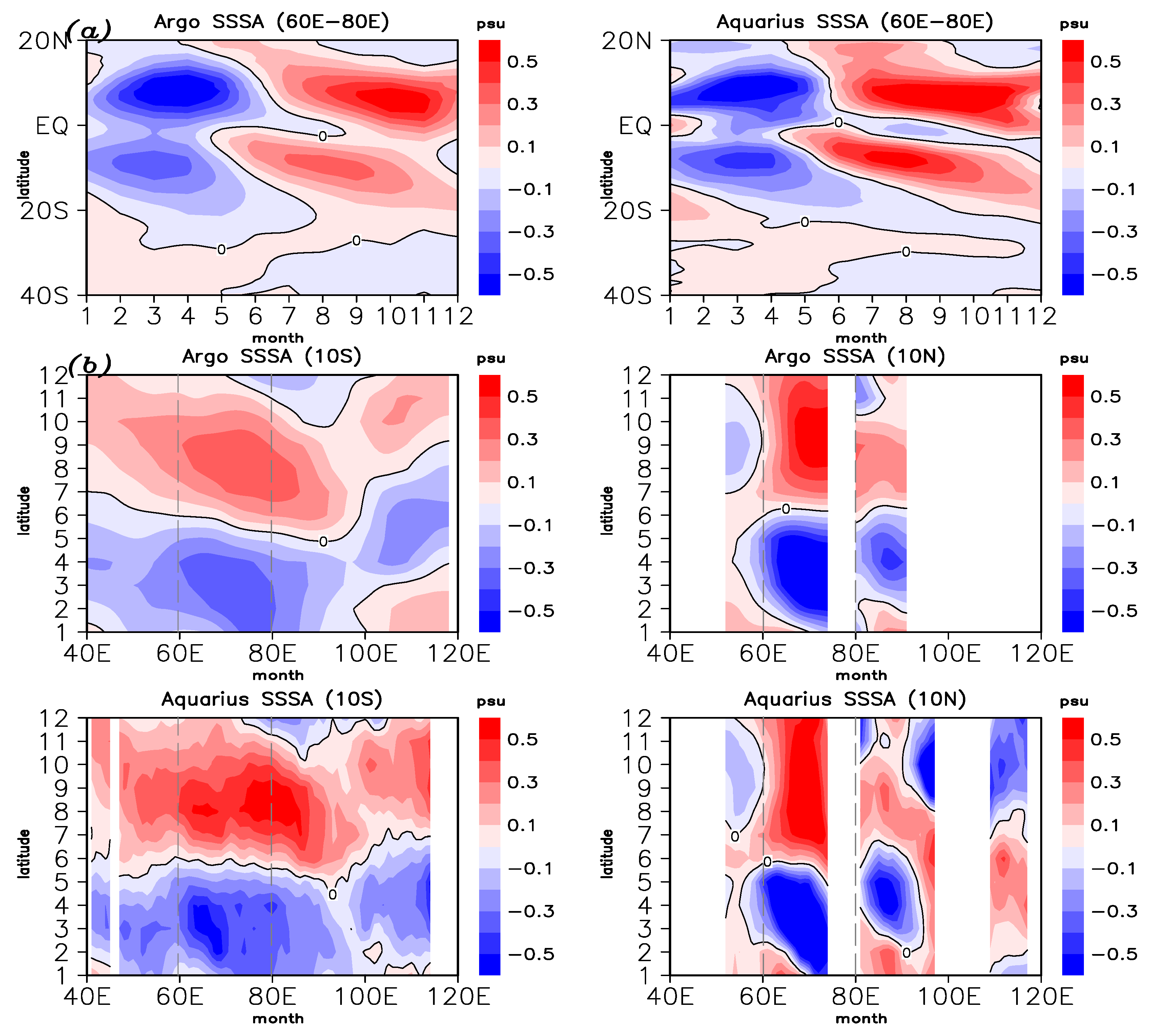
Figure 2a shows the latitude-time plots of SSSAs averaged over E–E, clearly depicting the positive SSSAs in May. The equator acts as a natural boundary, separating the changes in the SSSAs in the northern and southern Indian Ocean. There is an apparent time lag in these changes occurring across the southern to the northern Indian Ocean, which is consistent with the seasonal variability of the Indian Ocean induced by solar insolation. In this work, the SSSAs ESF area is defined as being the area of (S–S) and its corresponding SSSAs in the northern hemisphere (N–N) is also studied. Moreover, since the thermocline is shallower in the southwestern Indian Ocean and deeper in the eastern Indian Ocean and the easterlies are along the equator, the downwelling Rossby wave acts to suppress the continuous upwelling in the western Indian Ocean [39,40]. The symmetrical variability of SSSAs mode (Figure 2a) probably attributes to this downwelling Rossby wave [27,29,41]. However, there are no significant westward SSSAs motions along 10S and 10N in the hovmöller diagrams (Figure 2b). The maxima (minima) centres of SSSAs mainly locate in the SSSAs ESF areas. Consequently, the seasonal variability of SSSAs may be influenced by local atmospheric circulations and will be analysed in Section 5. But before doing so, we will examine next the relationship between SSSAs and SSTAs.
4. The Relationship between SSSAs and SSTAs before the Onset of SASM
The SSSA ESF area corresponds roughly with the Seychelles Dome (SD) which is a remarkable oceanic thermal dome along (E–E, 5°S–10°S) [42,43]. Due to its unique location, which is under the control of both the monsoon wind and south-easterly trade wind, SD has a semi-annual cycle associated with upwelling in the boreal spring [42,43]. Above the SD, sea surface temperature anomalies (SSTAs) are sensitive to variability in the upwelling and this is especially so in its seasonal variation [44].
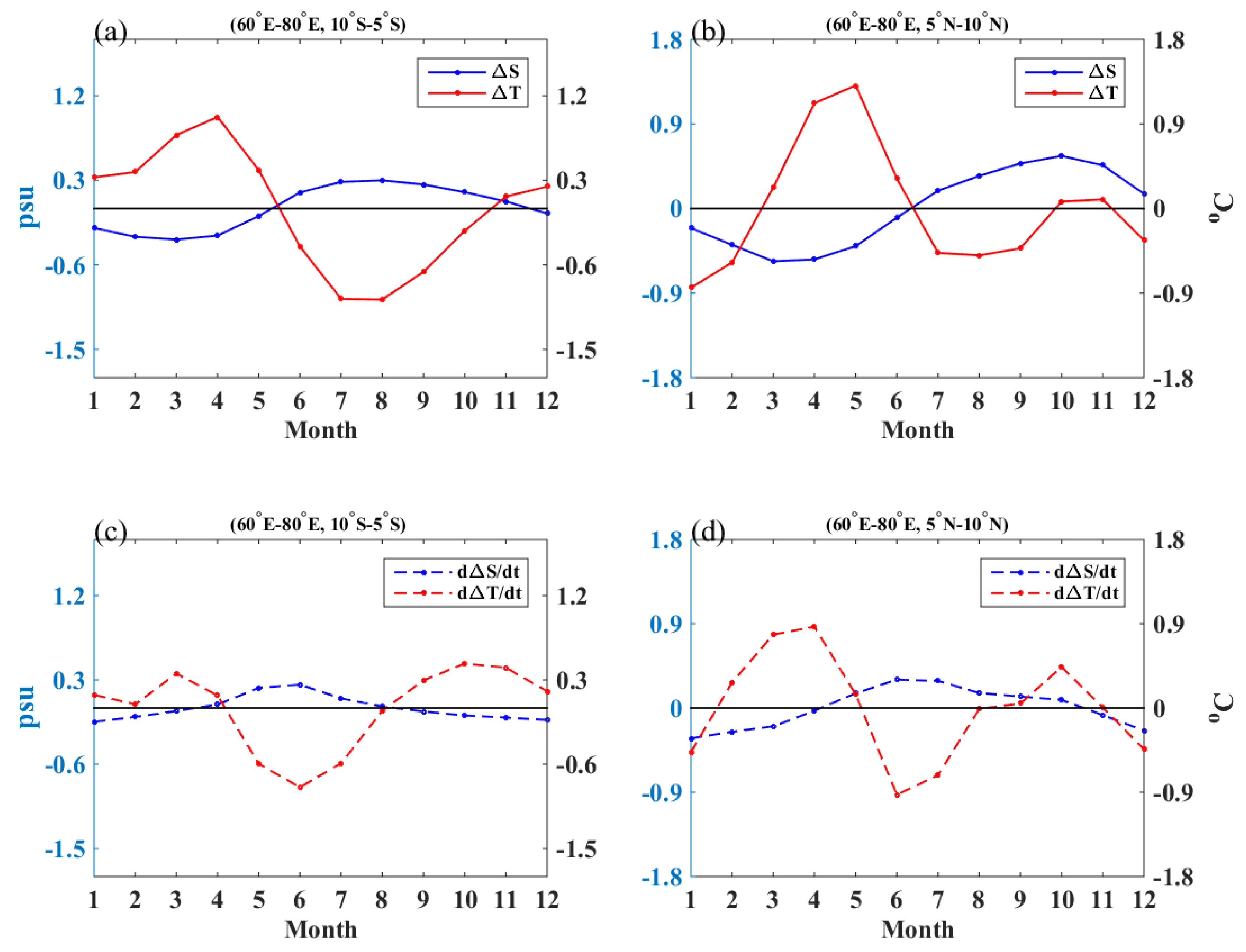
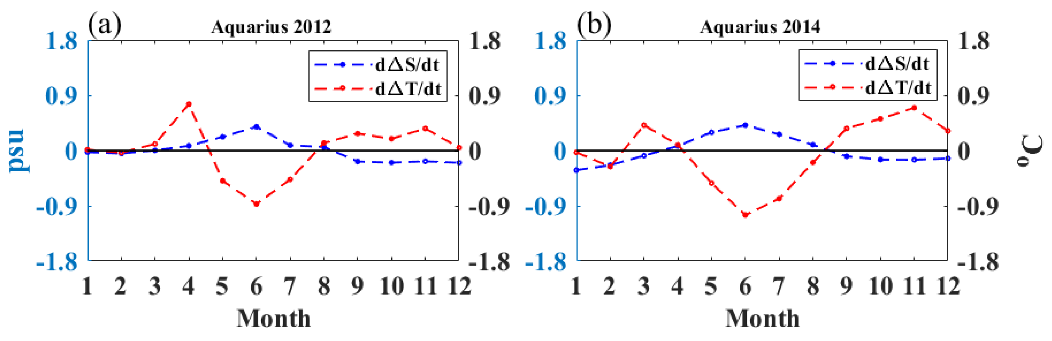
The seasonal variability of SSSAs is different from that of SSTAs, presenting not only in the trend of changing [when SSSAs increase, corresponding SSTAs decrease (Figure 3)] but also in the time of changing. Specifically, in the southern Indian Ocean, the tendency of SSSAs increases in the middle of March and that of SSTAs decreases in the early April. In the northern Indian Ocean, the tendency of SSSAs increases in the early April and that of SSTAs decreases in the early May. In other words, SSSAs have one and a half cycle/yr while SSTAs have one cycle/yr. Thus, SSSAs change faster than SSTAs. To give more convincing evidence of the quick change of SSSAs, we also calculated the seasonal variation in SSSAs and SSTAs for individual years with the Aquarius SSS dataset (Figure 4). Remarkably, the change of SSSAs tendency precedes that of SSTAs even in the individual years, except for 2013 (figure not shown), when the MJO (Madden Julian Oscillation) is very active during the onset of the SASM [45], resulting in heavy precipitation inhibiting SSSAs increase.
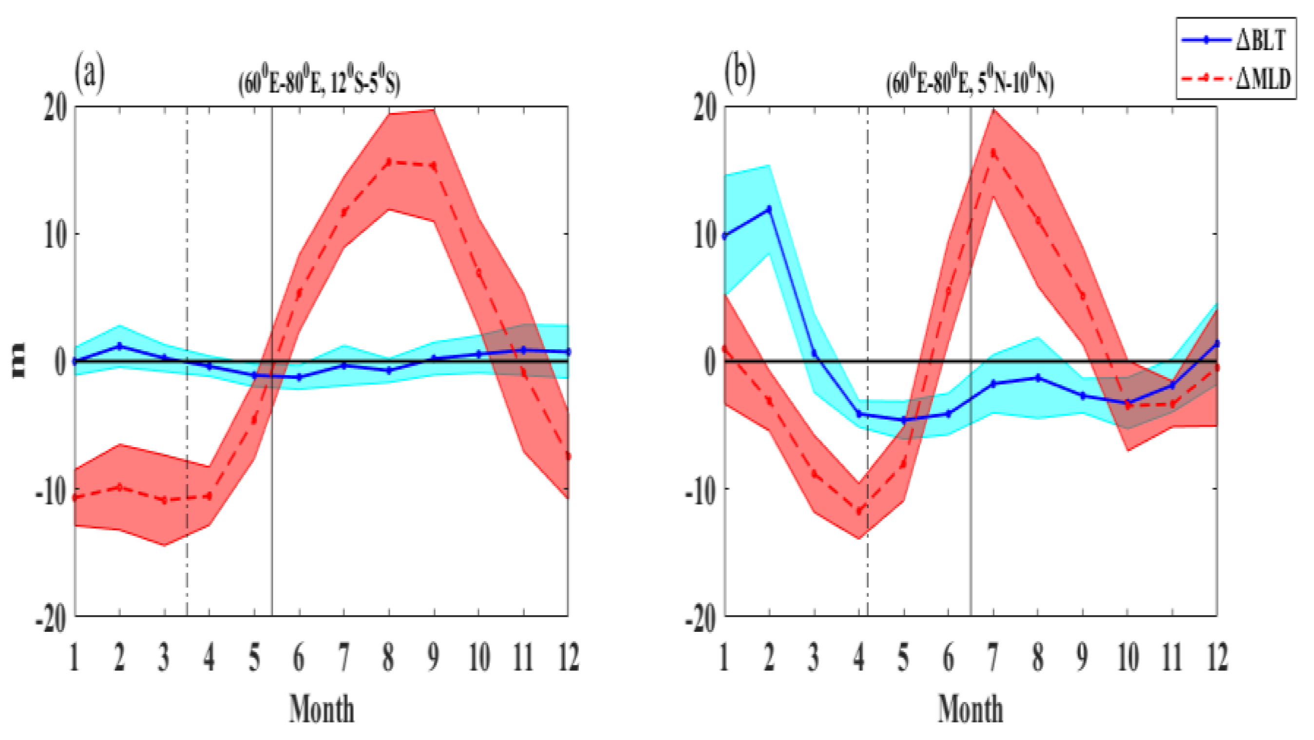
The earlier changed SSSAs may affect the oceanic stratification and, in turn, trigger a response in atmospheric circulation. To investigate this process, we show the seasonal variabilities of MLD and BLT anomalies in Figure 5. The top layer is the MLD which is defined as the depth that has a density change of 0.03 kg/m3 from the surface. In the SD area, the MLD anomalies change in the middle of May and are associated with the change of SSSAs and SSTAs (Figure 3a). BLT is the difference between an isothermal layer and the isopycnal MLD, insulating the surface from the deeper layers. Thereby, BLT has influences on the SST by controlling the vertical mixing [46,47]. In the SD area (Figure 5a), the change of BLT anomalies is more sensitive to the tendency of SSSAs rather than the seasonal variability of SSSAs (Figure 3c). When the tendency of SSSAs increase to positive in early March, the BLD anomalies begin to decrease below zero and vice versa. According to the calculation of BLT (in Section 2) and given the slightly decreasing MLD anomalies (Figure 5a), in the southern Indian Ocean, decreasing BLT anomalies are attributed to upwelling. Then, upwelling eats away at the BLT leading to more cold and salty water entrained into the mixed layer. When MLD anomalies increase in April, SSTAs begin to be affected by this upwelling process (the tendency of the SSTAs decrease below zero as shown in Figure 3c). In the northern Indian Ocean, things respond a little differently (Figure 5b). Although BLT and MLD also change in March, the tendency of SSSAs changes in April. We assume that this is because of the strong salty surface water in the Arabian Sea, so it needs more time for upwelling to affect the SSSAs. With the increasing SSSAs, the significantly decreasing BLT brings more subsurface water into the mixed layer, which in turn, promotes the decrease of SSTAs. As such, SSSAs has the potential ability to affect SSTAs through shoaling the BLT.
5. The External Forcing for the SSSAs Change
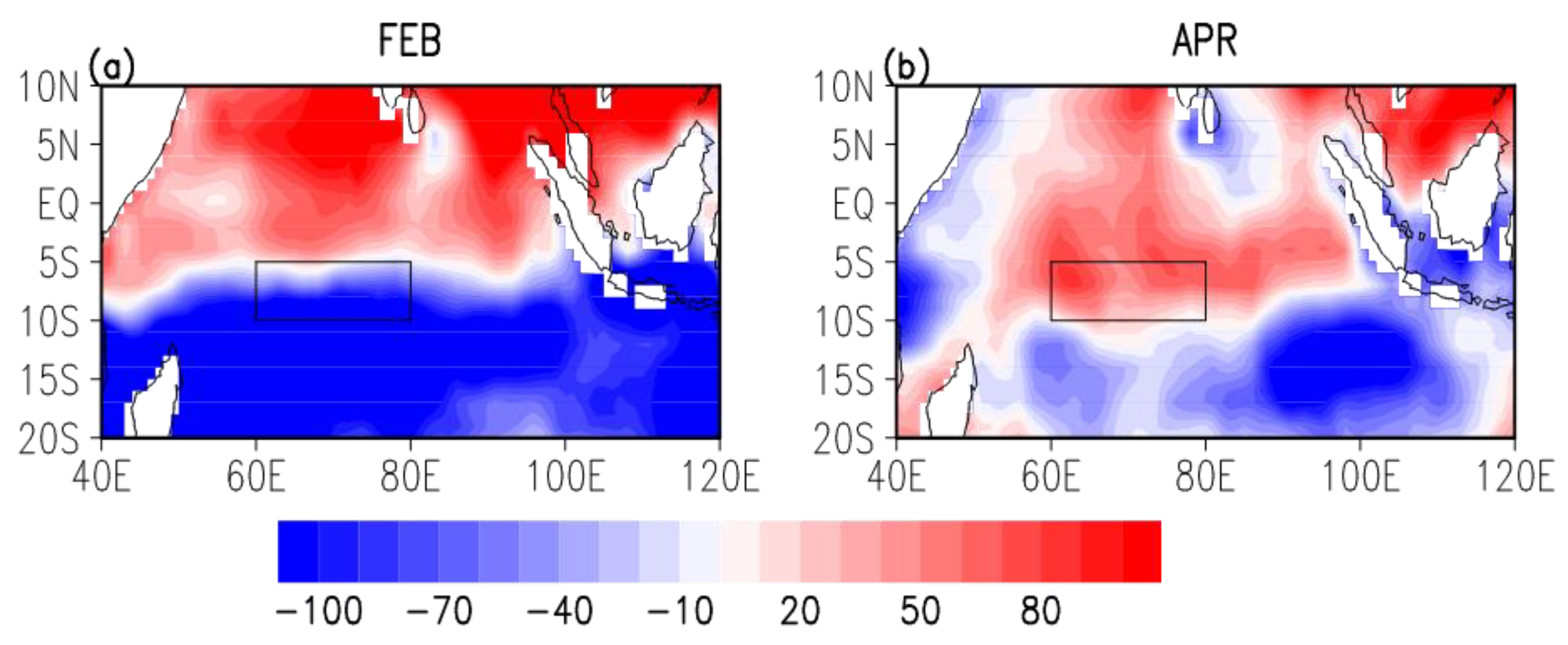
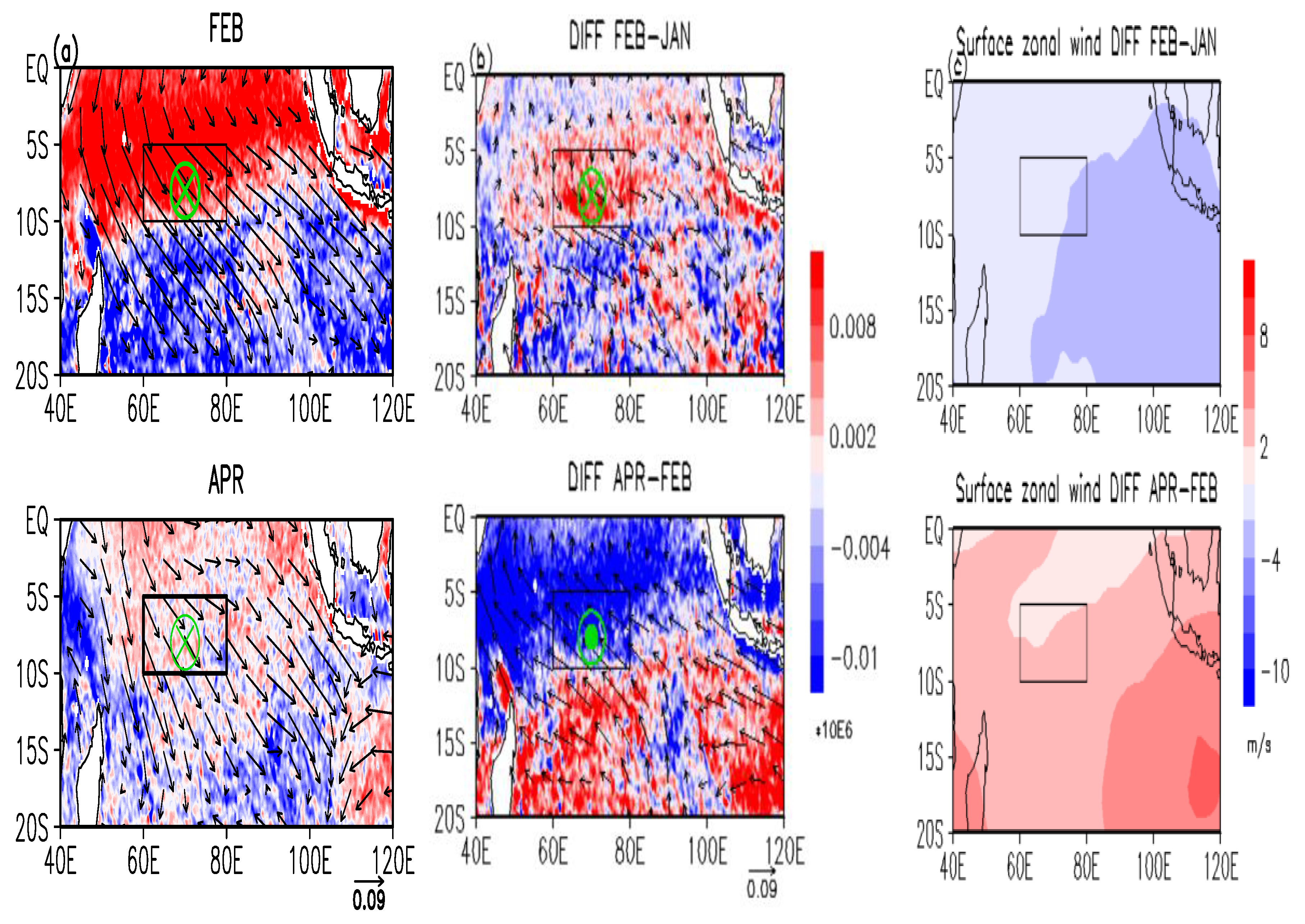
We analysed next the atmospheric circulation anomalies before and after the SSSAs change to better understand the variability of SSSAs. On the one hand, freshwater flux is stressed to play a crucial role in the seasonal variability of SSS in the Indian Ocean [12,19]. Figure 6 shows the distributions of freshwater flux anomalies in February and April respectively. Before the SSSAs change (February), there is more precipitation over the SSSA ESF area, while less freshwater goes into the SSSA ESF area after the SSSAs change (April); instead, strong evaporation anomalies make this area much saltier. On the other hand, the upwelling effect on the variability of SSSAs can be found in the entrainment circulations before and after the increasing SSSAs (Figure 7). The wintertime north-westerly wind anomalies intensify in the southern Indian Ocean before SSSAs change and weaken after SSSAs (Figure 7a). In the southern Hemisphere, negative curl corresponds to cyclonic curl and relative upwelling. Thereby, before the SSSAs change, the positive wind stress curl anomalies over the SSSAs ESF area, represent Ekman downwelling. After the SSSAs change, the negative wind stress curl anomalies induce Ekman upwelling in the SSSAs ESF area (Figure 7b). Furtherly, due to the negative wind stress curl anomalies in the north of 10S and the positive ones in the south of 10S before the increasing SSSAs (Figure 7b), corresponding to anticyclone in the north and cyclone in the south, the easterlies is strengthened (Figure 7c), which in turn, provides a favourable environment for upwelling in the eastern Indian Ocean. The mode of wind stress curl change after the SSSAs increasing, with positive anomalies in the north and negative in the south, leading to anomaly westerlies (Figure 7c). In March, the SSSAs increase just as the atmospheric circulation pattern begins to change into the SASM pattern and the thermocline in the SD starts to shoal as a result of weakened downwelling [44].
Therefore, freshwater flux and entrainment circulation anomalies contribute to the increasing SSSAs in the southwestern Indian Ocean.
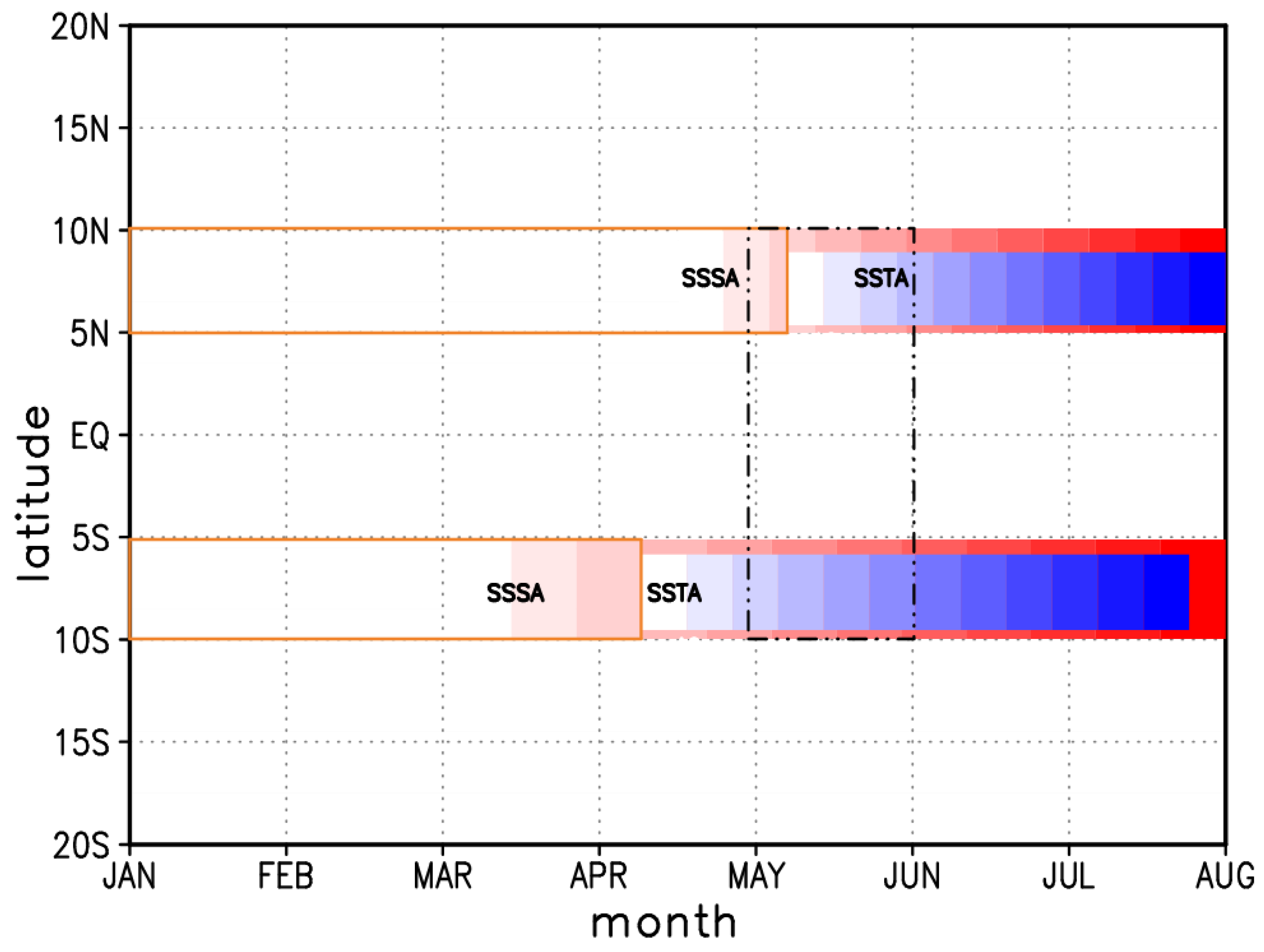
In summary (Figure 8), in the SD (S–S) from January to the early April, SSTAs stay in an increasing state (orange rectangle), while SSSAs start to increase in the middle of March (red filled rectangle), which is due to the less freshwater and Ekman upwelling caused by the wind stress. Thus increasing SSSAs, accompanied by the decreasing BLT anomalies, help to create a favourable environment for the SSTAs to decrease in the coming month via strengthening the upwelling. In other words, SSSAs, as one component in the ocean, are more sensitive in responding to the atmospheric influence than SSTAs. This phenomenon can also be found in the symmetrical area of the northern Hemisphere (N–N). One should mention here that there exist time-lags between the southern and northern Hemisphere, which leads to significant SST gradient in May (black rectangle). Thus, this heat contrast promotes the ITCZ to move northward and contributes to the change of vertical circulation.
6. Conclusions
In this study, we analysed the annual variability in sea surface salinity anomalies (SSSAs) by employing Aquarius satellite datasets from 2012 to 2014 and Argo datasets from 2005 to 2014, as well as the corresponding freshwater fluxes, sea surface temperature anomalies (SSTAs) and also ocean dynamic and atmospheric circulations.
We found that a positive SSSAs as an elongated spatial feature (ESF) along the equator in May with its area roughly coinciding with the Seychelles Dome (SD). The seasonal variability of SSSAs in the SD change from negative to positive and, in contrast, SSTAs change from positive to negative. Although their changes happen in spring, SSSAs change earlier than that of SSTAs, associated with the thinner barrier layer thickness (BLT) anomalies in the corresponding area, which in turn, help to provide favourable circumstance for the decreasing SSTAs. The change of SSSAs is closely related to the atmospheric circulation anomalies, mainly attributed to the freshwater flux anomalies and entrainment anomalies. Moreover, there exists a time delay of SSSAs change between the northern and the southern Indian Ocean, resulting in cross-equatorial current by forming the meridional SSTAs gradient. Therefore, SSSAs contribute to the onset of SASM by affecting the SSTAs.
Author Contributions
Conceptualization, Z.S. and X.Y.; Methodology, X.Y.; Software, X.Y.; Formal analysis, X.Y.; Writing—Original Draft Preparation, X.Y.; Writing—Review & Editing, Z.S., M.S.S. and X.Y.
Funding
This research received no external funding.
Acknowledgments
We thank three anonymous reviewers for their valuable comments. The authors also would like to thank the following data providers: The gridded ocean parameter datasets are available at the Asian-Pacific Data-Research Centre (http://apdrc.soest.hawaii.edu/data/data.php), NASA Jet Propulsion Laboratory (https://podaac.jpl.nasa.gov/announcements), Woods Hole Oceanographic Institution (http://oaflux.whoi.edu/evap.html), Climate Prediction Centre (http://www.esrl.noaa.gov/psd/data/gridded/data.cmap.html), National Oceanic and Atmospheric Administration (https://www.esrl.noaa.gov/psd/data/gridded/data.noaa.oisst.v2.html), the Centre de Recherche et d’Exploitation Satellitaire (http://cersat.ifremer.fr/data/products/latest-products) and Centre National D’études Spatiales (https://igsac-cnes.cls.fr/html/products.html). In addition, the reanalysis datasets are from the European Centre for Medium-Range Weather Forecasts (http://www.ecmwf.int/en/research/climate-reanalysis/era-interim).
Conflicts of Interest
The authors declare no conflict of interest. The founding sponsors had no role in the design of the study; in the collection, analyses, or interpretation of data; in the writing of the manuscript and in the decision to publish the results.
References
- Webster, P.; Fasullo, J. Monsoon: Dynamical theory. Encycl. Atmos. Sci. 2003, 3, 1370–1391. [Google Scholar]
- Jang, Y.; Straus, D.M. Tropical stationary wave response to ENSO: Diabatic heating influence on the Indian summer monsoon. J. Atmos. Sci. 2013, 70, 193–222. [Google Scholar] [CrossRef]
- Minoura, D.; Kawamura, R.; Matsuura, T. A mechanism of the onset of the South Asian summer monsoon. J. Meteorol. Soc. Jpn. 2003, 81, 563–580. [Google Scholar] [CrossRef]
- Shenoi, S.; Shankar, D.; Shetye, S. On the sea surface temperature high in the Lakshadweep Sea before the onset of the southwest monsoon. J. Geophys. Res. 1999, 104, 15703–15712. [Google Scholar] [CrossRef] [Green Version]
- Hénin, C.; Du Penhoat, Y.; Ioualalen, M. Observations of sea surface salinity in the western Pacific fresh pool: Large-scale changes in 1992–1995. J. Geophys. Res. Ocean. 1998, 103, 7523–7536. [Google Scholar] [CrossRef]
- Nyadjro, E.S.; Subrahmanyam, B.; Murty, V.; Shriver, J.F. The role of salinity on the dynamics of the Arabian Sea mini warm pool. J. Geophys. Res. Ocean. 2012, 117. [Google Scholar] [CrossRef] [Green Version]
- Schiller, A.; Mikolajewicz, U.; Voss, R. The stability of the North Atlantic thermohaline circulation in a coupled ocean-atmosphere general circulation model. Oceanogr. Lit. Rev. 1998, 1, 41–42. [Google Scholar] [CrossRef]
- Du, Y.; Zhang, Y. Satellite and Argo observed surface salinity variations in the tropical Indian Ocean and their association with the Indian Ocean Dipole mode. J. Clim. 2015, 28, 695–713. [Google Scholar] [CrossRef]
- Stammer, D. Global characteristics of ocean variability estimated from regional TOPEX/POSEIDON altimeter measurements. J. Phys. Oceanogr. 1997, 27, 1743–1769. [Google Scholar] [CrossRef]
- Sun, S.; Lan, J.; Fang, Y.; Gao, X. A triggering mechanism for the Indian Ocean Dipoles independent of ENSO. J. Clim. 2015, 28, 5063–5076. [Google Scholar] [CrossRef]
- Thompson, B.; Gnanaseelan, C.; Salvekar, P. Variability in the Indian Ocean circulation and salinity and its impact on SST anomalies during dipole events. J Mar. Res. 2006, 64, 853–880. [Google Scholar] [CrossRef]
- Vinayachandran, P.N.; Nanjundiah, R.S. Indian Ocean sea surface salinity variations in a coupled model. Clim. Dyn. 2009, 33, 245–263. [Google Scholar] [CrossRef]
- Grunseich, G.; Subrahmanyam, B.; Wang, B. The Madden-Julian oscillation detected in Aquarius salinity observations. Geophys. Res. Lett. 2013, 40, 5461–5466. [Google Scholar] [CrossRef] [Green Version]
- Guan, B.; Lee, T.; Halkides, D.J.; Waliser, D.E. Aquarius surface salinity and the Madden-Julian Oscillation: The role of salinity in surface layer density and potential energy. Geophys. Res. Lett. 2014, 41, 2858–2869. [Google Scholar] [CrossRef] [Green Version]
- Horii, T.; Ueki, I.; Ando, K.; Hasegawa, T.; Mizuno, K.; Seiki, A. Impact of intraseasonal salinity variations on sea surface temperature in the eastern equatorial Indian Ocean. J. Oceanogr. 2015, 72, 313–326. [Google Scholar] [CrossRef]
- Simon, B.; Rahman, S.; Joshi, P. Conditions leading to the onset of the Indian monsoon: A satellite perspective. Meteorol. Atmos. Phys. 2006, 93, 201–210. [Google Scholar] [CrossRef]
- Williams, P.D.; Guilyardi, E.; Madec, G.; Gualdi, S.; Scoccimarro, E. The role of mean ocean salinity in climate. Dyn. Atmos.Ocean. 2010, 49, 108–123. [Google Scholar] [CrossRef]
- Rao, R.R. Seasonal variability of sea surface salinity and salt budget of the mixed layer of the north Indian Ocean. J. Geophys. Res. 2003, 108, 3009. [Google Scholar] [CrossRef]
- Zhang, Y.; Du, Y. Seasonal variability of salinity budget and water exchange in the northern Indian Ocean from HYCOM assimilation. Chin. J. Oceanol. Limn. 2012, 30, 1082–1092. [Google Scholar] [CrossRef]
- Dong, S.; Garzoli, S.L.; Baringer, M. An assessment of the seasonal mixed layer salinity budget in the Southern Ocean. J. Geophys. Res. Ocean. 2009, 114. [Google Scholar] [CrossRef] [Green Version]
- Da-Allada, C.; Alory, G.; Du Penhoat, Y.; Kestenare, E.; Durand, F.; Hounkonnou, N. Seasonal mixed-layer salinity balance in the tropical Atlantic Ocean: Mean state and seasonal cycle. J. Geophys. Res. Ocean. 2013, 118, 332–345. [Google Scholar] [CrossRef] [Green Version]
- Neema, C.; Hareeshkumar, P.; Babu, C. Characteristics of Arabian Sea mini warm pool and Indian summer monsoon. Clim. Dyn. 2012, 38, 2073–2087. [Google Scholar] [CrossRef]
- Deshpande, R.; Muraleedharan, P.; Singh, R.L.; Kumar, B.; Rao, M.S.; Dave, M.; Sivakumar, K.; Gupta, S. Spatio-temporal distributions of δ 18 O, δD and salinity in the Arabian Sea: Identifying processes and controls. Mar. Chem. 2013, 157, 144–161. [Google Scholar] [CrossRef]
- Saraswat, R.; Nigam, R.; Mackensen, A.; Weldeab, S. Linkage between seasonal insolation gradient in the tropical northern hemisphere and the sea surface salinity of the equatorial Indian Ocean during the last glacial period. Acta Geol. Sin. 2012, 86, 1265–1275. [Google Scholar]
- Sijikumar, S.; Rajeev, K. Role of the Arabian Sea warm pool on the precipitation characteristics during the monsoon onset period. J. Clim. 2012, 25, 1890–1899. [Google Scholar] [CrossRef]
- Maes, C.; O’Kane, T.J. Seasonal variations of the upper ocean salinity stratification in the Tropics. J. Geophys. Res. Ocean. 2014, 119, 1706–1722. [Google Scholar] [CrossRef] [Green Version]
- Donguy, J.-R.; Meyers, G. Seasonal variations of sea-surface salinity and temperature in the tropical Indian Ocean. Deep Sea Res. Oceanogr. Res. Pap. 1996, 43, 117–138. [Google Scholar] [CrossRef]
- Rao, R.; Sivakumar, R. Seasonal variability of sea surface salinity and salt budget of the mixed layer of the north Indian Ocean. J. Geophys. Res. Ocean. 2003, 108, 3009. [Google Scholar] [CrossRef]
- Zhang, Y.H.; Du, Y. Seasonal variability of salinity budget and water exchange in the northern Indian Ocean from HYCOM assimilation. Chin. J. Oceanol. Limn. 2012, 30, 1082–1092. [Google Scholar] [CrossRef]
- Kao, H.; Lagerloef, G.; Lee, T.; Melnichenko, O.; Hacker, P. Aquarius Salinity Validation Analysis; Data Version 5.0. 2017. Available online: http://podaac-ftp.jpl.nasa.gov/allData/aquarius/docs/v5;AQ-014-PS-0016_AquariusSalinityDataValidationAnalysis_DatasetVersion5.0.pdf (accessed on 21 August 2018).
- Bhaskar, T.V.; Jayaram, C. Evaluation of Aquarius sea surface salinity with Argo sea surface salinity in the Tropical Indian Ocean. Geosci. Remote Sens. Lett. IEEE 2015, 12, 1292–1296. [Google Scholar] [CrossRef]
- Ebuchi, N.; Abe, H. Evaluation of sea surface salinity observed by Aquarius. In Proceedings of the 2014 IEEE International Geoscience and Remote Sensing Symposium (IGARSS 2014), Quebec City, QC, Canada, 13–18 July 2014; pp. 4427–4430. [Google Scholar]
- Qu, T.; Song, Y.T.; Maes, C. Sea surface salinity and barrier layer variability in the equatorial Pacific as seen from Aquarius and Argo. J. Geophys. Res. Ocean. 2014, 119, 15–29. [Google Scholar] [CrossRef] [Green Version]
- Yu, L.; Jin, X.; Weller, R. Multidecade Global Flux Datasets from the Objectively Analyzed Air-sea Fluxes (OAFlux) Project: Latent and Sensible Heat Fluxes, Ocean Evaporation, and Related Surface Meteorological Variables; OAFlux Project Technical Report, OA-2008-01; Woods Hole Oceanographic Institution: Woods Hole, MA, USA, 2008; 64p. [Google Scholar]
- De Boyer Montégut, C.; Madec, G.; Fischer, A.S.; Lazar, A.; Iudicone, D. Mixed layer depth over the global ocean: An examination of profile data and a profile-based climatology. J. Geophys. Res. Ocean. 2004, 109. [Google Scholar] [CrossRef] [Green Version]
- Reynolds, R.W.; Rayner, N.A.; Smith, T.M.; Stokes, D.C.; Wang, W. An improved in situ and satellite SST analysis for climate. J. Clim. 2002, 15, 1609–1625. [Google Scholar] [CrossRef]
- De Boyer Montégut, C.; Mignot, J.; Lazar, A.; Cravatte, S. Control of salinity on the mixed layer depth in the world ocean: 1. General description. J. Geophys. Res. Ocean. 2007, 112. [Google Scholar] [CrossRef] [Green Version]
- Mignot, J.; de Boyer Montégut, C.; Lazar, A.; Cravatte, S. Control of salinity on the mixed layer depth in the world ocean: 2. Tropical areas. J. Geophys. Res. Ocean. 2007, 112. [Google Scholar] [CrossRef] [Green Version]
- Shinoda, T.; Hendon, H.H.; Alexander, M.A. Surface and subsurface dipole variability in the Indian Ocean and its relation with ENSO. Deep Sea Res. Oceanogr. Res. Pap. 2004, 51, 619–635. [Google Scholar] [CrossRef]
- Potemra, J.T. Contribution of equatorial Pacific winds to southern tropical Indian Ocean Rossby waves. J. Geophys. Res. Ocean. 2001, 106, 2407–2422. [Google Scholar] [CrossRef] [Green Version]
- Yuhong, Z.; Yan, D.; Shaojun, Z.; Yali, Y.; Xuhua, C. Impact of Indian Ocean Dipole on the salinity budget in the equatorial Indian Ocean. J. Geophys. Res. Ocean. 2013, 118, 4911–4923. [Google Scholar] [CrossRef] [Green Version]
- Izumo, T.; Montégut, C.B.; Luo, J.-J.; Behera, S.K.; Masson, S.; Yamagata, T. The role of the western Arabian Sea upwelling in Indian monsoon rainfall variability. J. Clim. 2008, 21, 5603–5623. [Google Scholar] [CrossRef]
- Yokoi, T.; Tozuka, T.; Yamagata, T. Seasonal variation of the Seychelles Dome. J. Clim. 2008, 21, 3740–3754. [Google Scholar] [CrossRef]
- Yokoi, T.; Tozuka, T.; Yamagata, T. Seasonal and interannual variations of the SST above the Seychelles Dome. J. Clim. 2012, 25, 800–814. [Google Scholar] [CrossRef]
- Pai, D.; Bhan, S. Monsoon 2013: A report (IMD Met. Monograph no: ESSO/IMD/SYNOPTIC MET/01-2014/15); India Meteorological Department, National Climate Center: Pune, India, 2014. [Google Scholar]
- Maes, C.; Picaut, J.; Belamari, S. Importance of the salinity barrier layer for the buildup of El Niño. J. Clim. 2005, 18, 104–118. [Google Scholar] [CrossRef]
- Masson, S.; Luo, J.J.; Madec, G.; Vialard, J.; Durand, F.; Gualdi, S.; Guilyardi, E.; Behera, S.; Delécluse, P.; Navarra, A. Impact of barrier layer on winter-spring variability of the southeastern Arabian Sea. Geophys. Res. Lett. 2005, 32, 193–222. [Google Scholar] [CrossRef]
Figure 1.
Seasonal variability of sea surface salinity in the Indian Ocean. The annual cycle of sea surface salinity anomalies by (a) Aquarius dataset during 2012–2014 and (b) Argo dataset during 2005–2014. A, B and C (see January) denotes the eastern part (AEIO), the central part (BCIO) and the western part (CWIO) of the Indian Ocean respectively.


Figure 2.
Time-latitude diagrams (a) of SSSAs between E and E and hovmöller diagrams (b) of SSSAs along the area of 10S and 10N in Argo and Aquarius (Unit: psu, the dashed lines enclose the SSSAs ESF areas).
Figure 2.
Time-latitude diagrams (a) of SSSAs between E and E and hovmöller diagrams (b) of SSSAs along the area of 10S and 10N in Argo and Aquarius (Unit: psu, the dashed lines enclose the SSSAs ESF areas).

Figure 3.
Seasonal variability and tendency for both SSSA (obtained from Argo, in blue) and SSTA (obtained from NOAA; in red) in the areas [(a,c); E–E, S–S] and [(b,d); E–E, N–N] for 2005 to 2014. Unit: psu; C.
Figure 3.
Seasonal variability and tendency for both SSSA (obtained from Argo, in blue) and SSTA (obtained from NOAA; in red) in the areas [(a,c); E–E, S–S] and [(b,d); E–E, N–N] for 2005 to 2014. Unit: psu; C.

Figure 4.
Same as Figure 2 but for SSS data obtained from Aquarius.
Figure 4.
Same as Figure 2 but for SSS data obtained from Aquarius.

Figure 5.
Seasonal variability for both BLT (in blue) and MLD anomalies (in red) in the areas [(a); E–E, S–S] and [(b); E–E, N–N] for 2005 to 2014 (The shaded areas are the standard deviation, the solid black line represents the time that SSSAs change and dotted black line represents the time that the tendency of SSSAs change). Unit: m.

Figure 6.
Freshwater flux anomalies. (a) Monthly mean freshwater flux in February (a) and April (b) from 2005 to 2014. (Unit: cm/yr). The box (in black line) denotes the SSSAs ESF area (E–E, S–S).
Figure 6.
Freshwater flux anomalies. (a) Monthly mean freshwater flux in February (a) and April (b) from 2005 to 2014. (Unit: cm/yr). The box (in black line) denotes the SSSAs ESF area (E–E, S–S).

Figure 7.
Wind stress and wind stress curl anomalies. (a) Monthly mean wind stress (vector) and wind stress curl anomalies (shaded) in February and April from 2008 to 2014. (b) Differences in wind stress and wind stress curl anomalies as February minus January and April minus February, respectively. (Unit: N/m2; N/m3). (c) Differences in the surface zonal wind (10m) obtained from ERA-interim difference as February minus January and for April minus February, respectively (Unit: m/s). [The boxes in black line are the SSSAs ESF area in the southern Indian Ocean (E–E, S–S); the green plus mark represents downwelling and the green closed circle represents upwelling].

Figure 8.
Diagram of the potential mechanism between SSSA and the onset of SASM along E–E (Gradually increasing red rectangles represent the increasing SSSA and the blue ones represent the decreasing SSTA; In addition, the orange hollow rectangles represent the increasing SSTA and the black dot-dashed rectangle indicates the period with large SSTA gradient).

© 2018 by the authors. Licensee MDPI, Basel, Switzerland. This article is an open access article distributed under the terms and conditions of the Creative Commons Attribution (CC BY) license (http://creativecommons.org/licenses/by/4.0/).
Share and Cite
MDPI and ACS Style
Yuan, X.; Salama, M.S.; Su, Z. An Observational Perspective of Sea Surface Salinity in the Southwestern Indian Ocean and Its Role in the South Asia Summer Monsoon. Remote Sens. 2018, 10, 1930. https://doi.org/10.3390/rs10121930
AMA Style
Yuan X, Salama MS, Su Z. An Observational Perspective of Sea Surface Salinity in the Southwestern Indian Ocean and Its Role in the South Asia Summer Monsoon. Remote Sensing. 2018; 10(12):1930. https://doi.org/10.3390/rs10121930
Chicago/Turabian StyleYuan, Xu, Mhd. Suhyb Salama, and Zhongbo Su. 2018. "An Observational Perspective of Sea Surface Salinity in the Southwestern Indian Ocean and Its Role in the South Asia Summer Monsoon" Remote Sensing 10, no. 12: 1930. https://doi.org/10.3390/rs10121930
Note that from the first issue of 2016, this journal uses article numbers instead of page numbers. See further details here.