Capabilities of Chinese Gaofen-3 Synthetic Aperture Radar in Selected Topics for Coastal and Ocean Observations


1
Key Laboratory of Digital Earth Science, Institute of Remote Sensing and Digital Earth, Chinese Academy of Sciences, Beijing 100094, China
2
Laboratory for Regional Oceanography and Numerical Modeling, Qingdao National Laboratory for Marine Science and Technology, Qingdao 266235, China
3
Hainan Key Laboratory of Earth Observation, Sanya 572029, China
4
University of Chinese Academy of Sciences, Beijing 101408, China
*
Author to whom correspondence should be addressed.
Remote Sens. 2018, 10(12), 1929; https://doi.org/10.3390/rs10121929
Submission received: 1 October 2018
/
Revised: 9 November 2018
/
Accepted: 28 November 2018
/
Published: 30 November 2018
(This article belongs to the Special Issue Sea Surface Roughness Observed by High Resolution Radar)
Abstract
:Gaofen-3 (GF-3), the first Chinese spaceborne synthetic aperture radar (SAR) in C-band for civil applications, was launched on August 2016. Some studies have examined the use of GF-3 SAR data for ocean and coastal observations, but these studies generally focus on one particular application. As GF-3 has been in operation over two years, it is essential to evaluate its performance in ocean observation, a primary goal of the GF-3 launch. In this paper, we offer an overview demonstrating the capabilities of GF-3 SAR in ocean and coastal observations by presenting several representative cases, i.e., the monitoring of intertidal flats, offshore tidal turbulent wakes and oceanic internal waves, to highlight the GF-3’s full polarimetry, high spatial resolution and wide-swath imaging advantages. Moreover, we also present a detailed analysis of the use of GF-3 quad-polarization data for sea surface wind retrievals and wave mode data for sea surface wave retrievals. The case studies and statistical analysis suggest that GF-3 has good ocean and coastal monitoring capabilities, though further improvements are possible, particularly in radiometric calibration and stable image quality.
1. Introduction
A major reason that synthetic aperture radar (SAR) is favored for many applications in ocean observations is its high spatial resolution as an imaging radar. Simply put, SAR images allow us to observe the fine structures of many interesting oceanic and atmospheric phenomena and processes. Furthermore, as an active radar, SAR has the capability to work independent of sunlight and the ability to penetrate cloud cover and, to some extent, rain. Despite the short 106-day lifetime of the first civil ocean SAR onboard the SEASAT mission, it showed great potential for spaceborne SAR ocean observations [1]. The successful launch by the European Space Agency (ESA) of ERS-1 in 1991 and ERS-2 in 1995, both of which had onboard SAR sensors, enabled the operational acquisition of data for a long period of twenty years. In the 1990s, together with the ERS-1 and 2 SARs, another C-band SAR, Radarsat-1 (launched in 1995) and an L-band SAR, JERS-1 provided a large and diverse body for earth observations and significantly advanced our knowledge of the ocean, coastal zones, and polar regions.
The ocean is vast, with high spatial variability, therefore, it is preferable for spaceborne SAR to capture images with a large swath in addition to good spatial resolution. During the last century, the Radarsat-1 and Advanced SAR (ASAR) have acquired images with a swath width over a few hundred kilometers. Wide-swath or ScanSAR images generally have a spatial resolution of tens of meters and, more importantly, can map a large area of the open sea and coast, which makes them particularly suitable for studying meso-scale oceanic and atmospheric processes, e.g., by mapping the distribution of internal ocean waves [2], observing atmospheric solitons [3], estimating the wind speed of tropical cyclones [4], and measuring sea surface velocity [5].
The year 2007 marks an important advance in the development of spaceborne SAR; two X-band spaceborne SAR, the TerraSAR-X (TSX) and Cosmo-SkyMed and the C-band SAR, Radarsat-2 (R2), were launched. Compared with previous spaceborne SAR missions, the new generation of SAR sensors has several advantages. One advantage is that the new generation can acquire images with a high spatial resolution of up to 1 m in spotlight mode [6,7,8]. This offers a unique opportunity to detect targets in the ocean and coast, e.g., for ship detection [9,10,11]. The other advantage is that these SAR sensors have polarimetric capabilities of acquiring data in different polarization combinations of VV, HH, VH and HV. These SAR polarimetric data are widely exploited for oil spill detection or classification [12,13,14], analysis of objects scattering or their classification in coastal intertidal flats [15,16,17], and sea ice detection and classification [18,19,20]. In addition to the general advantages of the aforementioned high spatial resolution and polarimetry, advanced SARs have constellation configuration design. The Cosmo-SkyMed, TSX/TanDEM-X (TDX) and Sentinel-1A/1B missions, as well as the forthcoming Radarsat Constellation Mission (RCM), all operate in constellations, which significantly reduces the temporal intervals of SAR data acquisition and therefore enhances the capture of dynamic sea surface information [21,22,23]. In particular, TSX can cooperate with its twin, TDX, to achieve along-track interferometry and to retrieve sea surface currents in high spatial resolution from space [24].
During the development of spaceborne SAR, the wave mode of the ESA’s SAR missions has played an interesting role in ocean observations. These missions acquired “imagettes” (small size images, approximately 5–10 by 5–10 km) continuously over the global oceans and they are dedicated to ocean wave measurements, as the name indicates. The wave mode began during the ERS/SAR mission [25,26,27,28] and became operationally available for public users with the delivery of standard Level-1b (single-look-complex data) and Level-2 (swell spectrum) products. Along with the ASAR wave mode data, available from October 2002 to April 2012, statistical analysis of global ocean waves using these data provides additional insight into, e.g., ocean swell propagation and crossing in global oceans [29]. The current Sentinel-1A/1B SAR missions are continuing to acquire wave mode data with a larger image size of 20 km by 20 km and alternative incidence angles of 23° and 36° [30]. Since the Sentinel-1 wave mode image size is comparable to standard stripmap images, and these images are acquired globally and consecutively, we can expect wider applications in ocean observations based on these data. Besides the wave mode data of Sentinel-1A/1B acquired in global ocean, the Interferometry Wide (IW) swath (250 km) and Extra-Wide (EW) swath (400 km) modes data are acquired intensively in European water for ocean monitoring, as well as in polar regions for sea ice monitoring. Both the image modes employ the TOPSAR (Terrain Observation with Progressive Scans SAR, [31]) technique to avoid scalloping [32] and generate homogenous SAR images in large coverage. This technique can lead to better sea surface wind retrievals and the Sentinel-1A/1B sea surface wind products (one of the OCN products) become operationally available.
In August 2016, the Chinese first civil spaceborne SAR, named Gaofen-3 (a phonetic rendition of the Chinese word for “high spatial resolution”), joined the list of spaceborne SAR missions in orbit. Several studies have used GF-3 for ocean monitoring, mainly focusing on sea surface wind and wave retrievals. In [33], 56 data pairs of GF-3 collocations with buoy measurements were used to preliminarily assess the quality of sea surface wind retrieval; the results indicated a root-mean-square-error (RMSE) of 2.46 m/s. Ren et al. [34] conducted a more detailed analysis of sea surface wind retrieval from GF-3 Quad-Polarization Stripmap (QPS) data, not only in the VV but also HH and HV polarizations. An empirical algorithm was proposed in [35] to derive significant wave height (SWH) from GF-3 wave mode data. In total, 12 coefficients of the empirical algorithm were tuned using the collocations of the GF-3 wave mode data with the WaveWatch III mode results. However, it seems that only cut-off information derived from the GF-3 data [36] may also yield a reasonable SWH compared with the rather complicated empirical algorithm in [35].
After over two years of operation, GF-3 has acquired a large amount of global data; therefore, an overall assessment of its data quality and potential applications is essential. In this paper, we provide an overview of GF-3’s capabilities in ocean and coastal observations, focusing on presenting representative cases over a few “super” test sites where similar studies have been conducted using other spaceborne SAR data, to evaluate the full polarimetry, high spatial resolution and wide-swath imaging capabilities of GF-3. We also address the quantitative retrieval of sea surface wind and wave information from GF-3 data. Although some studies on wind and wave retrieval from GF-3 data have been reported, as previously mentioned, it is important to conduct an intensive investigation on how accurately we can derive sea surface wind and wave parameters from GF-3 data.
This paper is organized as follows. Section 1 presents a brief introduction of GF-3. Section 2 provides some representative examples of the use of GF-3 for ocean and coastal observations. In Section 3, we focus on evaluating data for sea surface wind and wave retrievals. Finally, conclusions and an outlook are given in Section 4.
2. Brief Introduction of GF-3
GF-3, which was launched by the “Long March 4C” rocket on 10 August 2016, operates in C-band (5.3 GHz) at an altitude of 755 km in a polar sun-synchronous orbit. The repeat cycle of the orbits is 29 days. Currently, four ground stations in China are receiving the GF-3 SAR data, the Miyun station (in the Beijing suburb), Kashi station (in Xinjiang, western China), Sanya station (in Hainan, southern China) and Mudanjiang station (in the northeastern China), as well as an overseas station in Kiruna, Sweden.
GF-3 has flexible imaging modes. The five general modes are spotlight, stripmap, ScanSAR and wave. GF-3 also has several subclasses for the various general imaging modes. For example, the stripmap mode has standard stripmap, quad-polarization stripmap and fine stripmap modes. In addition, GF-3 can acquire data operationally in full polarization of VV (Vertical-Vertical), HH (Horizontal-Horizontal), VH and HV (Horizontal-Vertical) with various swath widths (up to 50 km) and spatial resolutions (up to 8 m). Table 1 lists the details of the available imaging modes of GF-3 and their technical specifications.
The standard GF-3 products include Level-1a single-look-complex data, Level-1b intensity data and so-called Level-2 projected and georeferenced intensity data. The data are stored in TIFF format for each polarization channel, and the ancillary information (i.e., the metadata) is stored in XML files, similar to the standard products of other present spaceborne SAR missions. Along with the rational polynomial coefficients (RPC) file, one can derive geolocation information for individual pixels of each GF-3 SAR image.
3. Uses of GF-3 for Coastal and Open Ocean Observations
In this section, representative cases including coastal observations of an intertidal flat and offshore wind farm turbulent wakes and open ocean observations of internal waves, are presented to demonstrate GF-3’s polarimetry, high spatial resolution and wide-swath imaging capabilities. Some of these cases are similar to previous studies using other spaceborne SAR data, such as TSX, Radarsat-2 and ENVISAT/ASAR.
3.1. Determination of the Scattering Characteristics of an Intertidal Flat in the Subei Shoal with GF-3 Full Polarimetric Data
To demonstrate the polarimetric capabilities of GF-3, we use an example from the Subei Shoal, which has unique radiation characteristics. Surface objects in the region include a complex mixture of mud flats, tidal current channels, aquaculture rafts and offshore wind farm turbines. Along with tidal variations, the radar backscatter characteristics of the objects in this area show high spatial and temporal variations in spaceborne SAR images, particularly in different polarization channels, as they have different scattering mechanisms. Therefore, the Subei Shoal is an appropriate site to test the polarimetric capability of SAR.
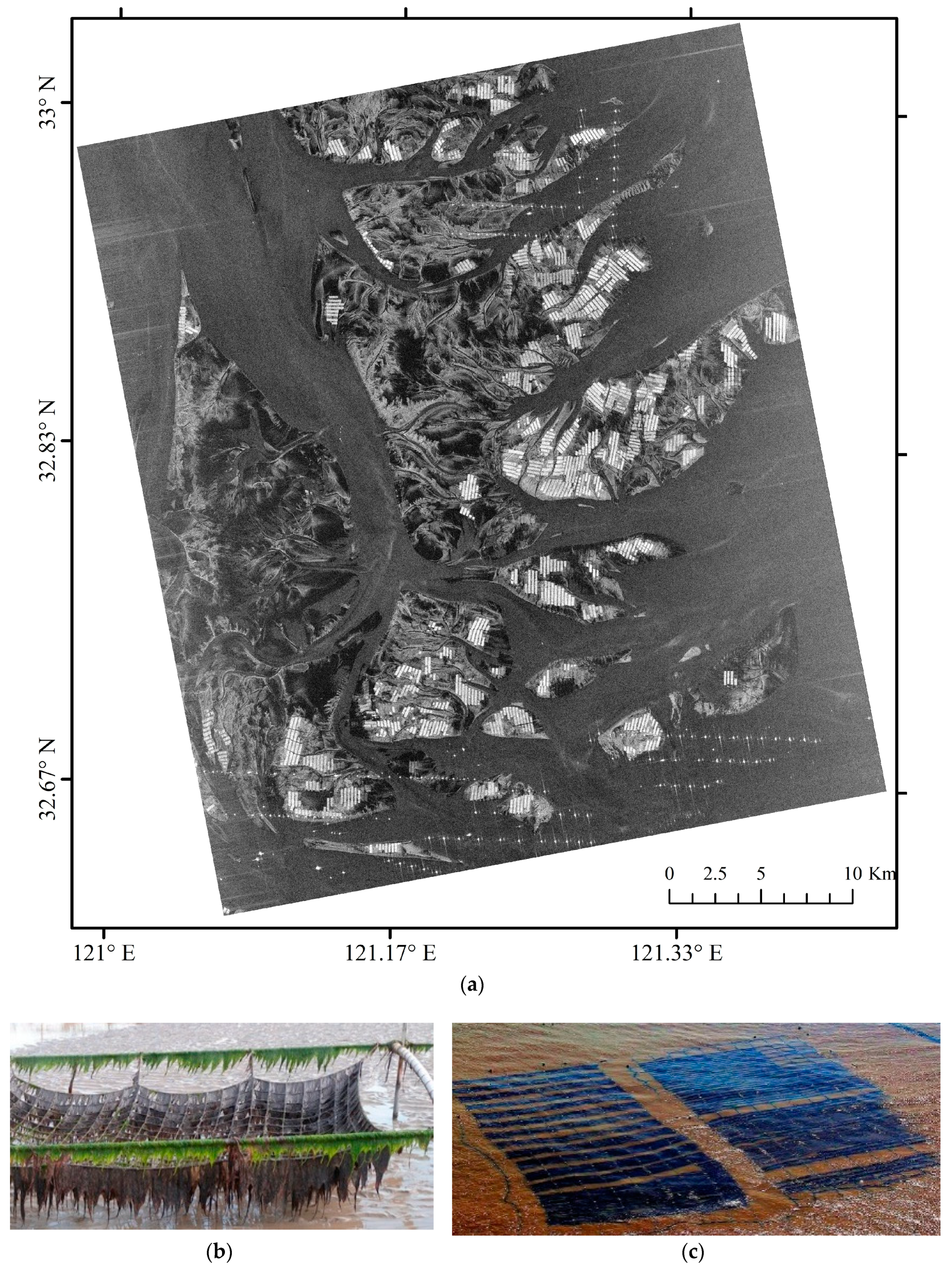
Figure 1a shows the radiometrically calibrated HV polarization from GF-3 Quad-Polarization Stripmap (QPS) data acquired on 5 October 2017. In the HV-polarized GF-3 SAR image, the distinct bright and ordered strip features are rafts composed of bamboo, ropes and nets for Porphyra aquaculture. Figure 1b is a photo of a single raft, while the photo in Figure 1c shows an array of numbers of rafts seen from sky. The unique structures of these rafts can induce strong volume scattering and therefore they are presented as bright patterns in the HV-polarized SAR image. The radar backscatter features of mud flats in the HV-polarized image are complicated, showing both bright and dark patterns. Thanks to high spatial resolution of the image, we can see the veering black lines, which are water channels in the mud flats.
In a previous study [16], by exploiting dual-polarization TSX data (HH and VV polarizations) and quad-polarization R2 data (VV, HH, VH and HV polarizations), we conducted a detailed analysis of the polarimetric characteristics of different objects in this area. Here, we apply the same method, i.e., the four-component scattering power decomposition [37] to GF-3 quad-polarization data to show various scattering characteristics of objects in the intertidal flat area. Figure 1d is false-color composite image from the GF-3 QPS data, using the four-component decomposition method where the red, blue and green channels represent the double bounce, surface and volume scattering, respectively. A brief description of the four-component scattering power decomposition method follows.
Equation (1) derives the Pauli vector of the polarimetric SAR data, and the coherency matrix is given in Equation (2):
where , , are the scattering matrix elements, and it is assumed that satisfies the reciprocity condition. The symbol 〈〉 denotes the ensemble average in an imaging window, and the superscript denotes the complex conjugation. The coherency rotation after a rotation by angle is obtained using Equation (3), as follows:
The rotated coherency matrix is further decomposed into four scattering components corresponding to the surface, double bounce, volume, and helix scattering mechanisms, as follows:
where , , and are the contributing coefficients, and , , , and are the decomposition powers for the surface, double bounce, volume and helix scattering mechanisms, respectively. To determine the dominant scattering mechanism from the decomposition results, each scattering component is normalized using Equation (6).
The decomposition result suggests that the polarimetric characteristics of the objects in this area are complex. The aquaculture rafts show highly variable polarimetric characteristics in different areas. Near the sea, they generally appear green in the false-color composite image, which indicates that volume scattering is dominant. This result is likely induced by the dense Porphyra attached to the rafts (see Figure 1b), as October–November is the high season for Porphyra aquaculture in the area [38]. Away from the sea, the water level decreases, and some rafts are exposed to the air; therefore, the dihedral angle between the bamboo grid of the rafts and the sea surface can induce double bounce scattering. Thus, they appear red and yellow (indicating a mixture of double bounce and volume scattering) in the false-color image. Some rafts even appear magenta, which suggests a mixture of double bounce and surface scattering. This phenomenon probably indicates few Porphyra attached on the rafts, so no volume scattering is induced.
An interesting feature is the yellow area in the left-hand part of the false color composition map, which indicates a mixture of double bounce and volume scattering in the mud flat, whereas the corresponding HV-polarized signal is very weak, as well as in other polarization channels. We do not have a plausible explanation for this feature. We conducted an in situ experiment in our previous study using TSX and R2 and found that visual inspection is very helpful for interpretation of polarimetric decomposition results in this area. However, in this case, we have only the SAR data and therefore, our analysis is mainly based on previous experience. The Subei Shoal is a unique area where both natural and man-made objects can show variable polarimetric characteristics due to changes in the tidal level and human activities. Further experiments to analyze the GF-3 polarimetric capabilities should focus on acquiring time-series data, as well as with essential field work to better understand the different polarimetric characteristic of various objects.
3.2. Observations of Offshore Wind Turbine Tidal Current Wakes
Numerous offshore wind farms have been constructed worldwide. The offshore wind turbine wake phenomenon is an important factor that needs to be considered for wind farm construction and operation. These wakes are generated because the turbine height, which often exceeds 90 m above the sea surface and the turbine’s rotation induces spirals downstream in the air. When the helix vortices “touch” the sea surface and modulate Bragg waves, the sea surface roughness is consequently changed; therefore, when these areas are imaged by SAR, they often appear dark [40]. Spaceborne SAR, due to its high spatial resolution as an image radar, demonstrates unique advantages in monitoring offshore wind turbine wakes in terms of determining wake length, deficit velocity and wake meandering [41,42].
Interestingly, the wakes in offshore wind farms observed by SAR are not always induced by the rotating turbine turbulence in the air. In a previous study [43], a TSX image acquired over the East China Sea offshore wind farm (near Shanghai) shows a distinct wake pattern downstream from each wind turbine. Based on multiple satellite observations and a numerical simulation, it was concluded that these patterns were generated by turbulence induced by interactions between the offshore wind farm foundation and a strong tidal current in Hangzhou Bay. Compared with the offshore wind turbine wakes generated by turbulence in the air, these wakes have a small spatial scale of approximately 500–1000 m in length, which varies with tidal current intensity and turbine foundation size. Therefore, these relatively small wakes are usually observed in SAR images with a high spatial resolution, e.g., in the TSX stripmap image with a spatial resolution of 3 m.
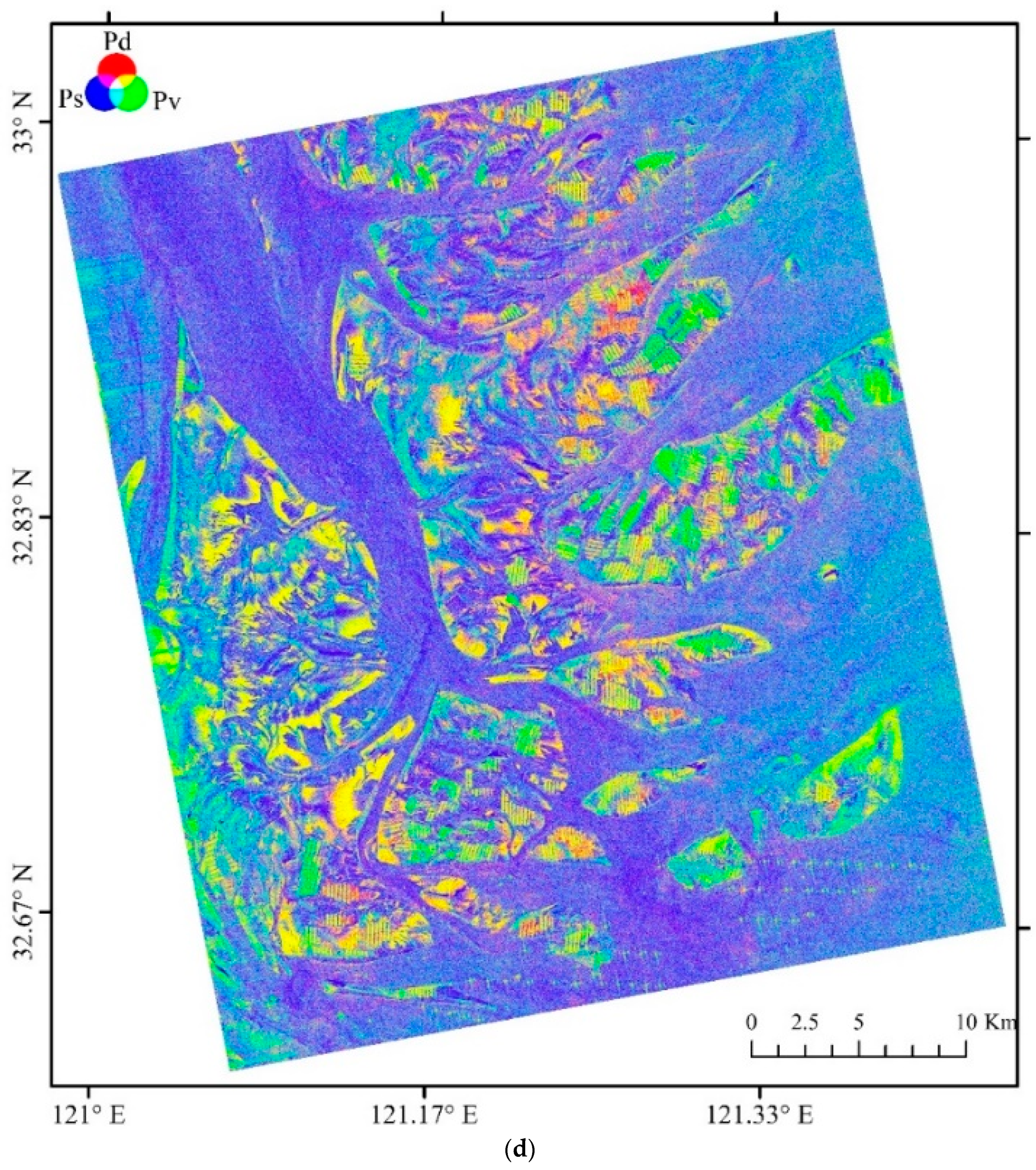
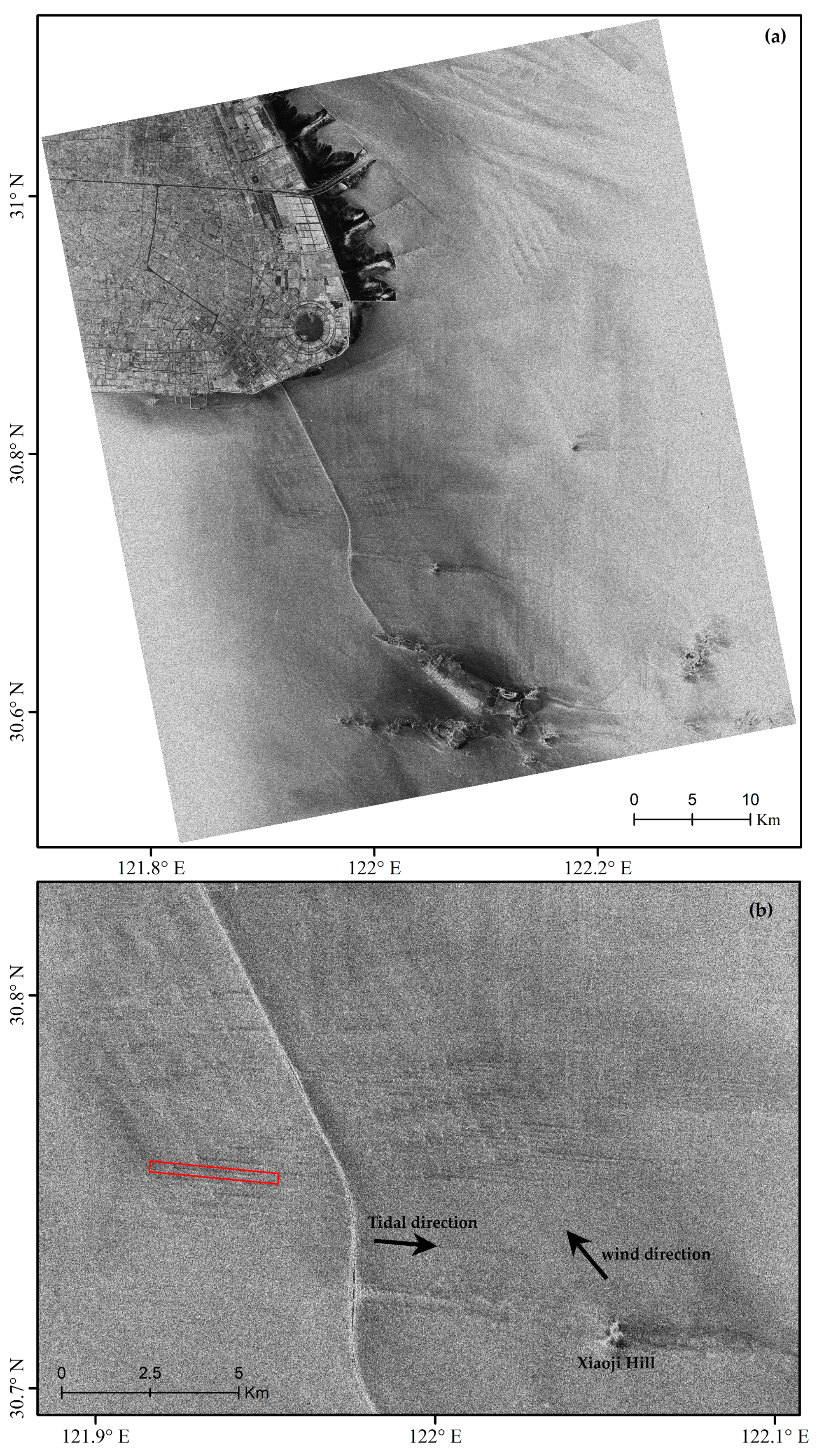
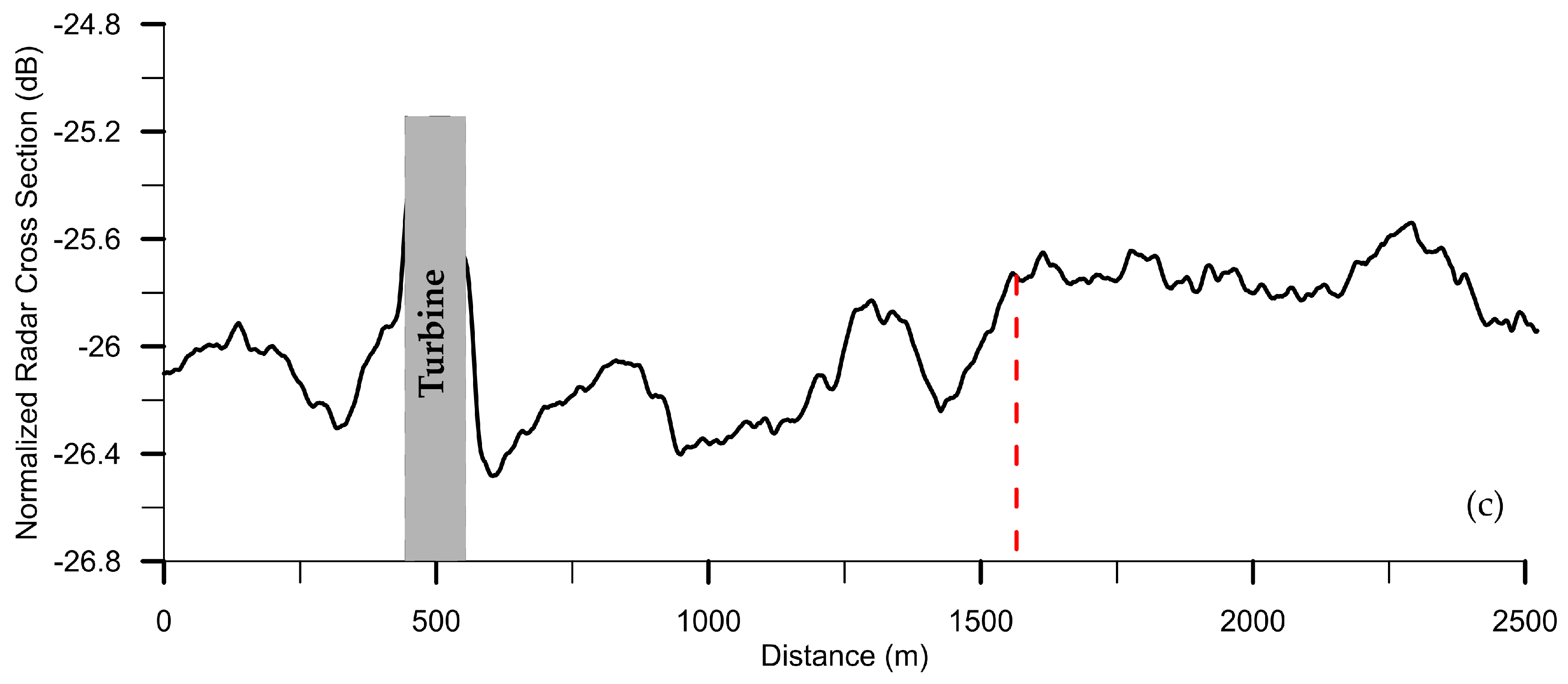
GF-3 has a fine stripmap image (FSI) mode, with a nominal spatial resolution of 5 m in both the azimuth and range directions. Figure 2a shows a GF-3 FSI image (HH polarization) acquired at 9:45 UTC on 15 February 2017, over the offshore wind farm in the East China Sea. The upper left part shows the urban area of Shanghai, and the upper right shows the Changjiang river estuary, where the visible linear features are induced by ebb tide currents. The wind farm is located to both the east and west of the Donghai Bridge (the veering line in the middle of the image). The sub-image in Figure 2b shows better visualization of sea surface features over the offshore wind farm area. In this sub-image, one can see linear patterns downstream of each offshore wind turbine with an approximately west-east orientation, whose lengths vary between 500 and 2000 m. One example of variations of the Normalized Radar Cross Section (NRCS) in the turbulent wake is shown in Figure 2c, which suggests that the NRCS gradually recovers downstream to a state comparable with that upstream of the turbine; therefore, the wake length is approximately 1000 m, as marked by the red dashed line in the figure. These patterns, which were induced by the water turbulence generated by the interaction between tidal currents and offshore wind turbine piles, are the same as those observed in a TSX image [41]. The piles are rounded, with diameters of approximately 15 m. In the southern part of the wind farm, there is a longer and more prominent wake pattern at the bridge induced by water turbulence from the interaction between tidal currents and the bridge piers. In the figure, we can also observe much longer bands, particularly apparent in the northwest of Xiaoji Hill, which are wind wakes. The European Centre for Medium-Range Weather Forecasts (ECMWF) ERA-interim model suggests the sea surface wind direction was approximately 320° at 9:00 UTC on 15 February 2017, which is consistent with northwest-southeast orientations of these wide and long bands, i.e., suggesting they are wind wakes.
Interestingly, we note that the sea surface wind direction in both the GF-3 and the TSX cases are cross with the tidal current direction. As previously discussed in the TSX case [43], wind stress plays an important role in the manifestation of the tidal current wake on SAR images. When the sea surface wind has a perpendicular component in the turbulent wake direction, it further enhances convergence and divergence of the wakes. This phenomenon represents one reason why the tidal current wakes in this case are not as distinct as those in the TSX case, because the sea surface wind speed of this case is approximately 6.0 m/s (ERA-Interim model result at 9:00 UTC) versus above 9.0 m/s in the TSX case. Second, the TSX case occurred closer to the spring tide and would have had a stronger tidal current than the GF-3 case. Finally, the TSX image has a steeper incidence angle of 19.7°–23.2° than that of the GF-3 of 23.9°–27.7° and therefore, one can generally expect strong radar backscattered signal. Moreover, the X-band SAR is more sensitive to the short scale Bragg waves than the C-band SAR, according to the Bragg resonant mechanism.
Compared with the wind wakes apparent in high resolution SAR images, the tidal current wakes have smaller spatial scales. While the former wakes often have a length greater than several kilometers (and up to tens of kilometers), the latter wakes generally have a length less than a few kilometers. The high spatial resolution capability of spaceborne SAR allows us to identify distinct tidal current wakes induced by man-made objects in shallow water. We note that these distinct wind farm turbulent wakes have also been identified in the North Sea offshore wind farm parks [44]. The promotion of clean offshore wind energy must not neglect the changes in local hydrodynamics [45] caused by wind farms and possible associated environmental issues.
3.3. Observation of Internal Waves in the South China Sea
It is generally understood that the internal waves (IWs) in the northeastern South China Sea (SCS) are primarily generated by interactions between barotropic tides and sills in the Luzon Strait; these IWs then propagate westward. Dongsha Atoll is in the pathway of these IWs in the northeastern SCS. The complicated bathymetry and various oceanic stratification patterns lead to significant spatial variations in IW at Dongsha Atoll.
The IW refraction, diffraction, reconnection and even reflection dynamics in Dongsha Atoll are all recorded by spaceborne SAR [46,47]. As there are often a few IW packets arriving at Dongsha Atoll with varying distances, and these IWs generally have long crests of a few hundred kilometers, it is preferable to use wide swath SAR images to clearly visualize IW propagation in this area. Therefore, Dongsha Atoll is a good site to test the capability of ocean surface imaging in wide swath by spaceborne SAR for observation of IW dynamics.
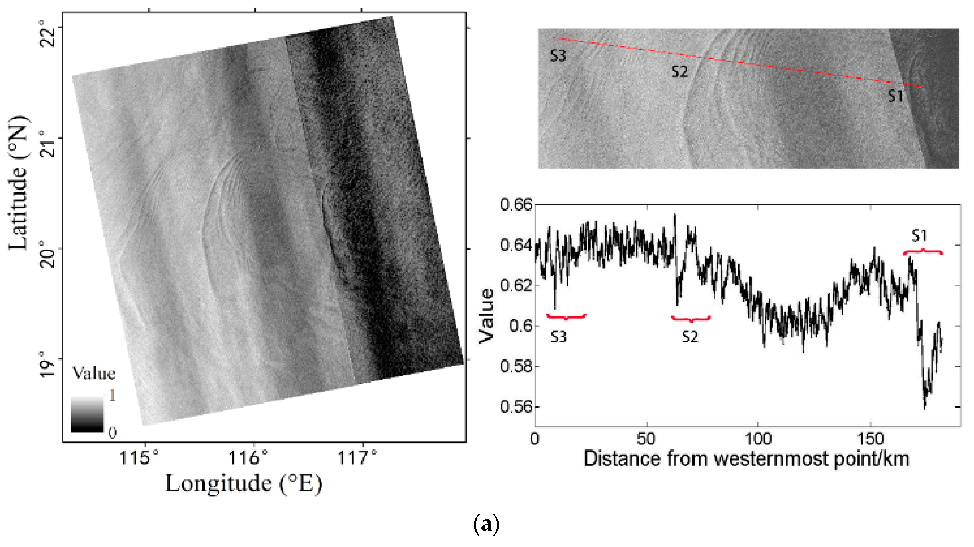
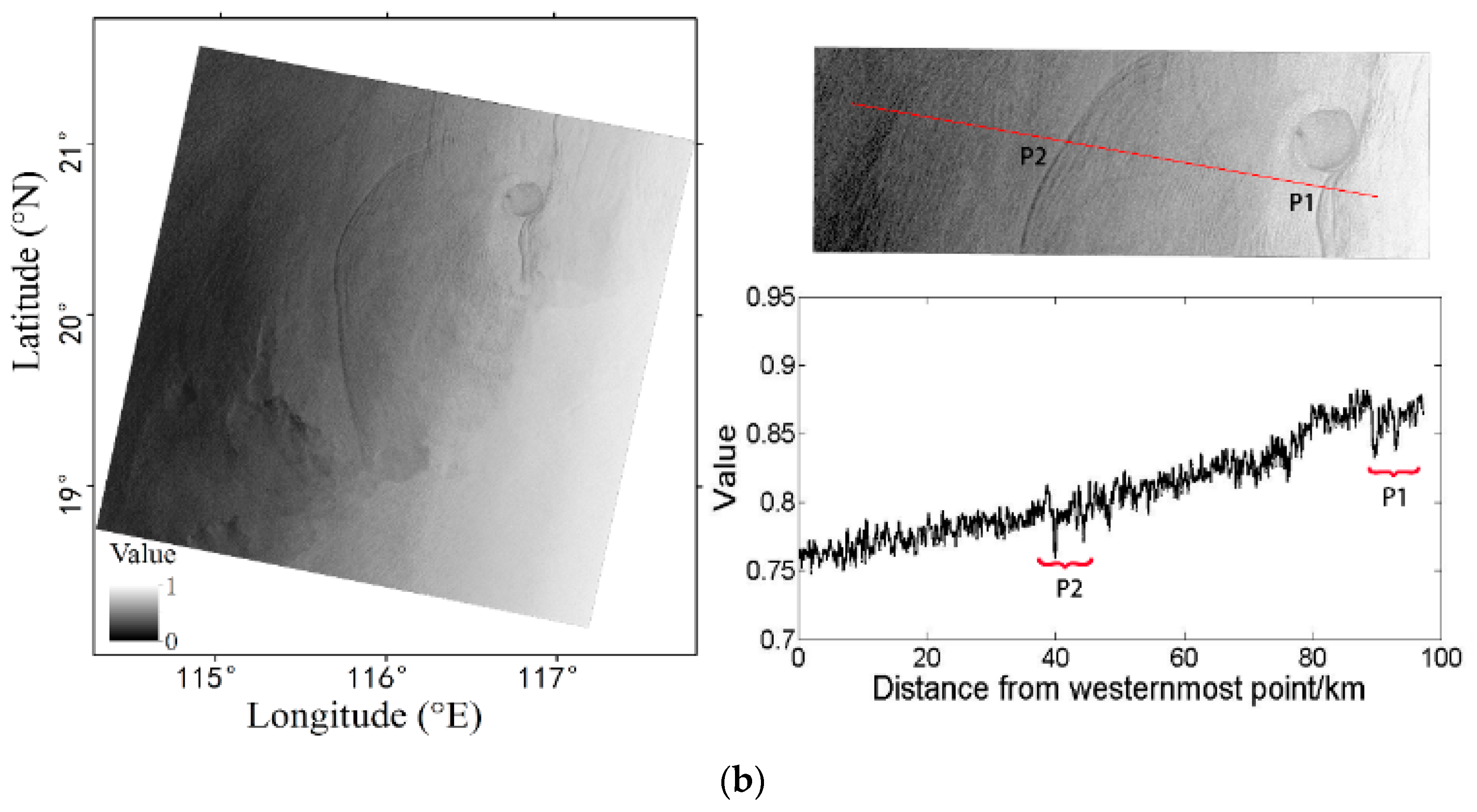
Figure 3 shows two GF-3 SAR images acquired in the narrow ScanSAR mode (three beams) with a swath width of approximately 300 km over Dongsha Atoll on 21 October and 24 October 2017, in ascending and descending orbits, respectively. The two images have almost identical spatial coverages. The clear arc-shape signatures of the internal solitary waves (ISWs) in the two SAR images reveal that the waves experienced significant spatial variations, i.e., wave refraction and diffraction, as they passed through Dongsha Atoll (as shown by the clearly visible round shape in the GF-3 image on 24 October). On the right side of Figure 3, the upper panels show two sub-images covering part of the ISW southern arms over Dongsha Atoll. The lower panels show the gray value variations in the GF-3 images across the transects through the ISW packets, indicated by the red lines in the two sub-images. Because IWs can induce convergence and divergence of sea surface flow, the sea surface roughness and radar backscatter are consequently changed because the Bragg waves are modulated by the sea surface flow [48]. Therefore, the significant changes in the image gray values suggests there are three IW packets (labeled S1, S2 and S3) in the 21 October 2017 image and two wave packets (labeled S1 and S2) in the 24 October 2017 image. The distance between neighboring ISW crests in one packet appears to monotonically decrease from front to rear, suggesting that these ISWs were propagating westward. As waves are assumed to propagate in the direction normal to the wave crests, it is estimated that the ISWs were traveling toward 272°–295° (clockwise relative to north). Variations in the gray values also suggest that the front section of the westward ISW is bright and the rear section is dark, indicating that the ISWs are depression waves. In the two SAR images, the distance between the leading wave crests P1 and P2 is approximately 107 km, close to the distance between S1 and S2, whereas the distance between P2 and P3 is 53 km. Li et al. noted that tidal daily inequality can lead to different inter-packet distances over Dongsha Atoll [49].
The ISWs in the northeastern SCS often have long crests up to a few hundred kilometers, appear in successive packets, and have spatial extents of a few hundred kilometers. Therefore, ScanSAR images are favorable for the observation of IWs in the SCS. The two images in Figure 3 yield a broad view of the dynamic ISW refraction and reconnection processes in Dongsha Atoll, highlighting the wide swath imaging capability of GF-3. However, some problems with the GF-3 ScanSAR image remain to be addressed. In the image acquired on 21 October, the rightmost beam presents a noticeable grayscale inhomogeneity compared with the two neighboring beams. In contrast, the image acquired on 24 October shows a homogeneous gray level transition from the SAR near to far range. Note that the two images were both radiometrically calibrated, although the normalized values are used for the current presentation. We were not able to eliminate the distinct sea surface radar backscatter inhomogeneity from beam to beam. While the image is suitable for qualitative analysis of IW dynamics, such inhomogeneities can lead to significant bias in quantitative retrieval of marine-meteorological parameters, such as sea surface wind speed, where absolute radar backscatter values are used.
4. Retrieval of Sea Surface Wind and Wave
In the previous sections, we present three cases demonstrating the full polarimetry, high spatial resolution and wide-swath imaging capabilities of GF-3. In this section, we examine GF-3’s performance in the quantitative retrieval of sea surface wind and wave.
4.1. Sea Surface Wind Retrieval Using QPS Mode Data
The QPS mode is a promising GF-3 SAR imaging mode that obtains surface radar backscatter in four polarization channels of VV, HH, VH and HV. In the previous section, we presented an analysis of surface object radar backscatter characteristics based on polarimetric decomposition using QPS mode data. SAR VV polarization data is preferable for sea surface wind retrieval, as the sea surface generally has stronger radar backscatter in VV than that in other polarization channels. However, the VV polarized signal becomes insensitive to sea surface wind speeds above 25 m/s. Recent studies have suggested that SAR cross-polarization signals (VH or HV) increase linearly with increasing sea surface wind speeds [50,51] and are less dependent on wind direction and incidence angle than the VV polarization data [52].
Therefore, we started with the QPS mode data for sea surface wind retrieval. Notably, QPS is among a few imaging modes with the largest volume of data acquired by GF-3 over the ocean. However, when we attempted to compare the sea surface wind speed derived from QPS VV polarized data with those derived from wind models or other satellite measurements, we found distinct discrepancies. As the retrieval of sea surface wind information using C-band SAR data in VV polarization is a mature method, i.e., a method based on the geophysical model function (GMF), which relates the radar backscatter cross section σ0 with the sea surface wind speed and direction and the radar incidence angles, we deduce that the σ0 values of the original GF-3 QPS mode data probably have some biases. Any SAR data used for quantitively deriving marine-meteorological parameters must be radiometrically calibrated well. Equation (7) is the general radiometric calibration procedure of SAR data given in the unit dB. The DN value is the digital number recorded by the instrument, and the external calibration constant (kcali_constant, positive values in Equation (7)) is provided in the SAR data annotation file.
To verify the accuracy of the GF-3 QPS mode data in VV polarization, we conducted a simulation experiment. As the C-band GMF (CMODs), can approximately reflect the sea surface radar backscatter σ0 of C-band SAR in VV polarization given the sea surface wind speed and direction, we used CMOD5.N to simulate the GF-3 QPS data σ0 for comparison. A total of 2841 QPS GF-3 SAR images acquired from September 2016 to November 2017 were collected. Each QPS image was divided into a few 5 km by 5 km subscenes, which were further collocated with the ECMWF ERA-Interim sea surface wind field (available every 3 h in a grid of 0.125°) (available at: http://apps.ecmwf.int/datasets/data/interim-full-daily/) using a temporal window less than 0.5 h and spatial distance less than 12.5 km. Next, the simulated σ0_sim was achieved by inputting the collocated ERA-Interim sea surface wind speed, direction and radar incidence angle of each scene into CMOD5.N.
The GF-3 SAR radar backscatter without radiometric calibration is denoted σ0_raw, which is equal to 10log10(DN2). Then, the difference between σ0_sim and σ0_raw, Δσ, was treated as the external calibration constant value, assuming the simulated σ0_sim is close to the truth of the normalized radar cross section and neglecting other factors that may affect the GF-3 radiometric calibration accuracy:
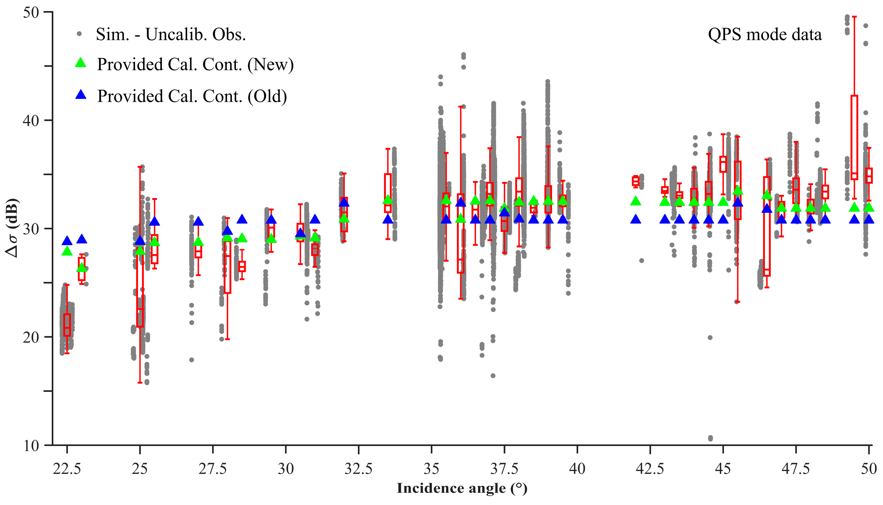
Figure 4 shows the diagram of variations in ∆σ with incidence angles. The gray dots are the ∆σ values of each collocated data pair, on which the whiskers are overlaid. The results show that the ∆σ values are scattered and the acquired data irregularly distributed at different incidence angles. According to Equation (8), in an ideal situation, the value of ∆σ should be equal to ; however, because the ∆σ values for each incidence angle are highly variable, we used the median values of the whiskers (red solid lines within the boxes) as . In the diagram, the overlaid blue triangles indicate the “old” calibration constants with respect to the “new” ones released in May 2018, which are marked by green triangles. The new calibration constants are generally higher than the old ones by an average of approximately 1.4 dB over different incidence angles. The recently updated calibration constants are close to the revised ones, i.e., , particularly for incidence angles ranging from 35° to 40°, where also the QPS mode data amount are the largest. The overall difference between the old calibration constants and , is 2.56 dB, whereas the difference between the new calibration constants and , decreased to 1.68 dB.
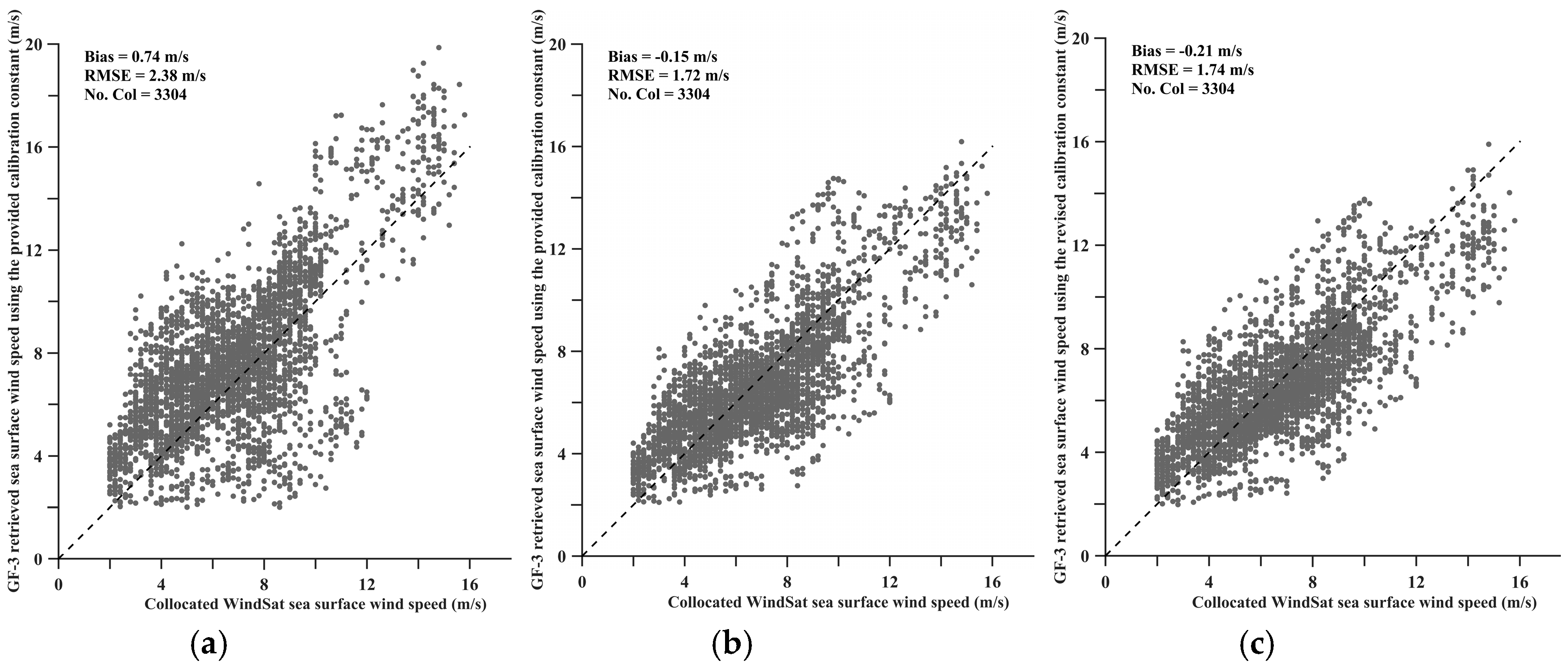
To further verify our assumption, the sea surface wind speeds were retrieved using the three groups of different calibration constants, which were collocated with WindSat sea surface wind speeds (available from http://www.remss.com/), treated as an independent dataset because the ERA-Interim data were used to derive . Figure 5 shows the comparison. When the old calibration constants were used, the comparison yields a large bias of 0.74 m/s and an RMSE of 2.38 m/s. When the new calibration constants were used, the bias and RMSE decrease to −0.15 m/s and 1.72 m/s, respectively; these results are similar to those achieved using the revised calibration constant for sea surface wind speed retrieval from GF-3, which has bias and RMSE values of −0.21 m/s and 1.74 m/s, respectively. The new calibration constants yield better retrievals, with results similar to those derived using the revised calibration constants. This suggests that continuous efforts to improve the accuracy of radiometric calibration are strongly recommended to achieve high quality sea surface wind retrieval results from GF-3 data.
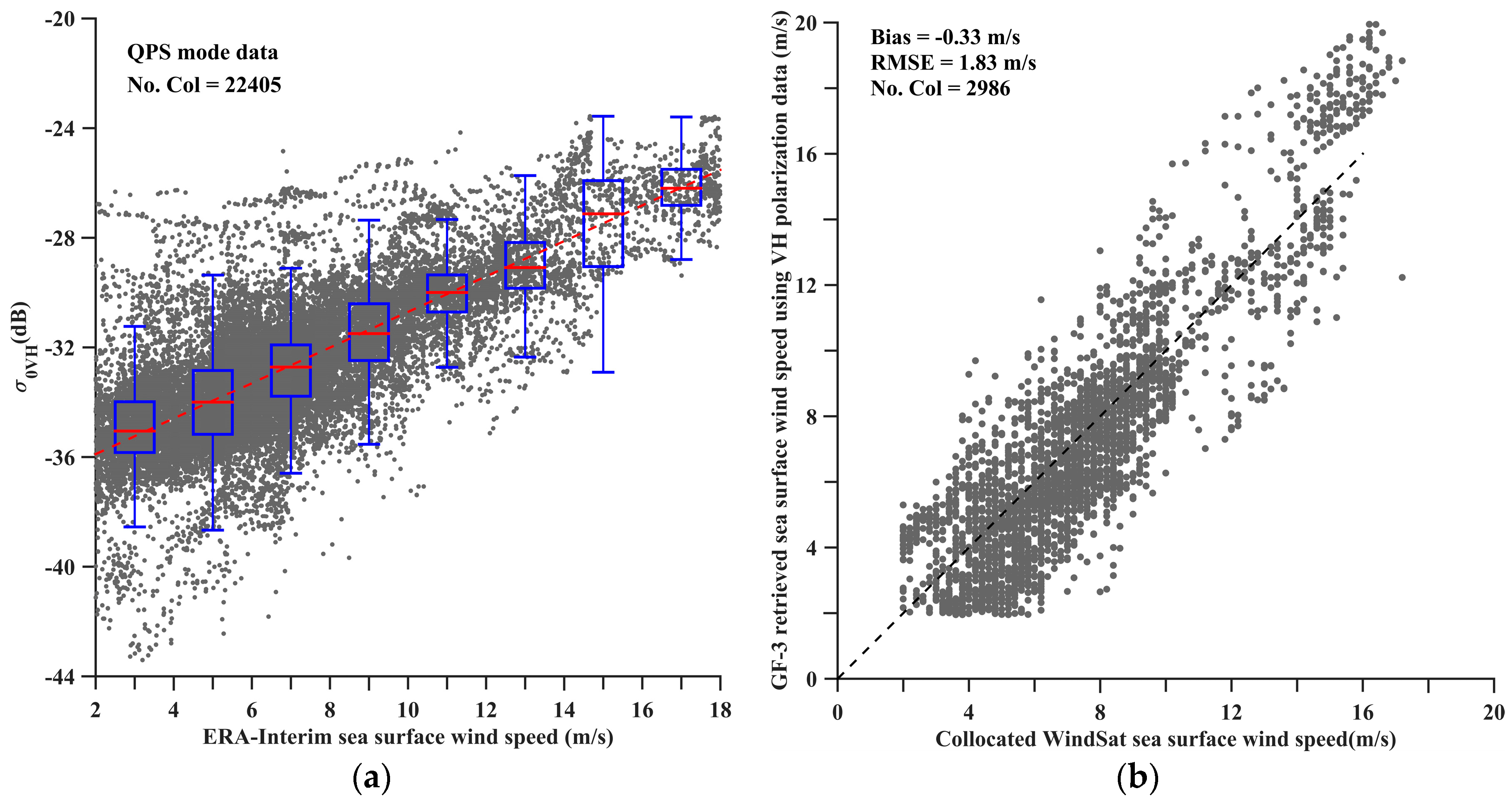
Following the analysis of sea surface wind speed retrieval from QPS VV polarization data, we further examined the possibility of deriving sea surface wind speeds from VH polarization data. In view of the analysis above, the newly released calibration constants of the VV polarization data yielded better retrieval results than the old calibration constants, which are close to the retrievals using our revised calibration constants. This suggests that the radiometric calibration accuracy is improved. Therefore, we used the new calibration constants to derive the normalized radar cross section of the QPS cross-polarization data. Next, the mean of the VH polarized data subscenes were collocated with the ECMWF ERA-Interim sea surface wind field, as shown in Figure 6a and the boxes and whiskers were overlaid on the scatter plot. The plot suggests some important information about the GF-3 QPS VH data radar backscatter. First, the lower extremes of the whiskers suggest that the noise sigma equivalent zero (NESZ) is approximately −38 dB, comparable with the R2 and Sentinel-1 values of −35 dB [50,53]. Furthermore, the median values suggest a linear increase in with sea surface wind speed, as indicated by the red dotted line. Thus, we fitted a linear relationship between and the sea surface wind speed, , as follows:
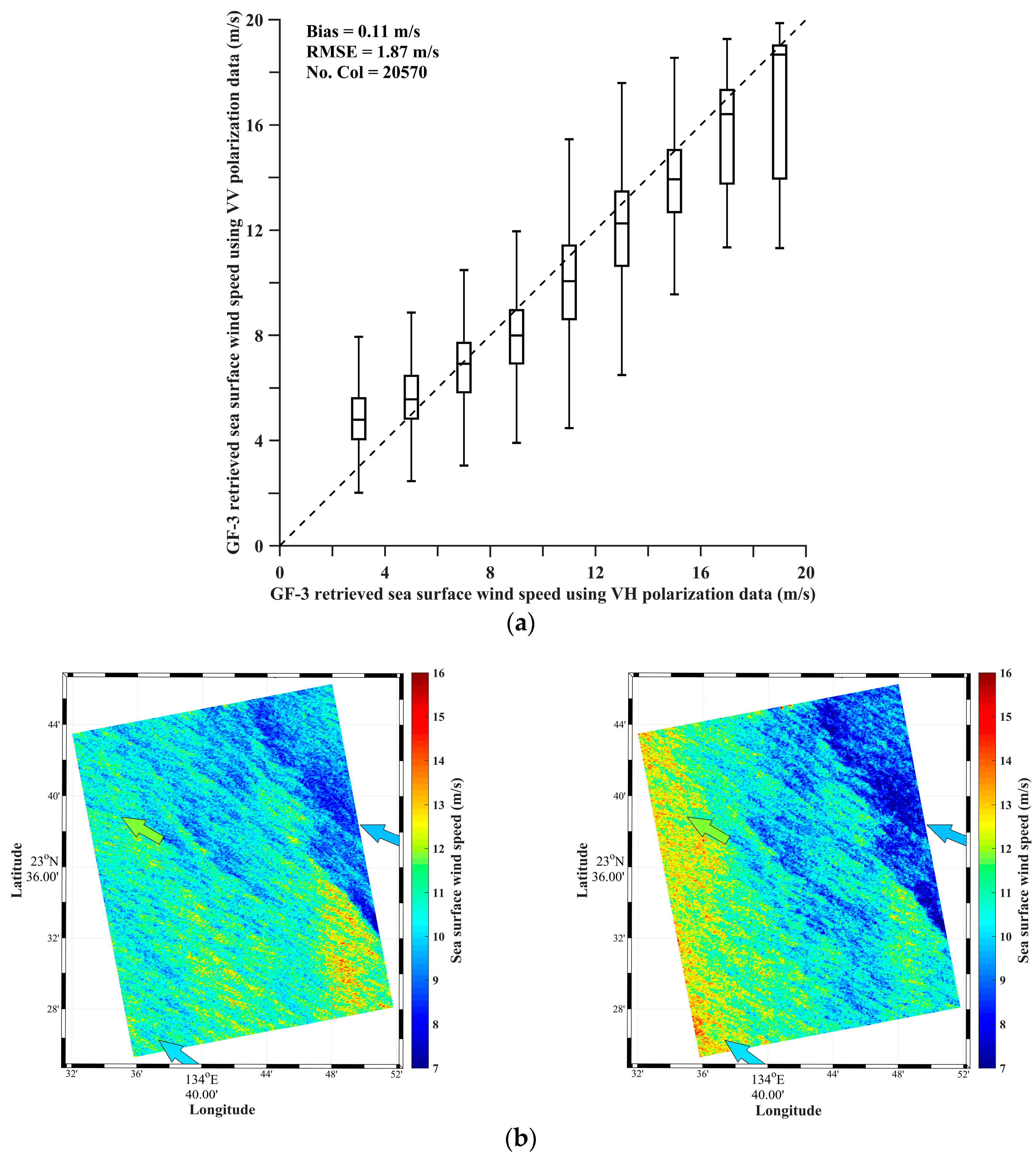
We then used the relationship to derive sea surface wind speed from the VH polarization data and compared them with the independent wind measurements from WindSat, as shown in Figure 6b. The comparison yielded a bias and an RMSE of −0.33 m/s and 1.83 m/s, respectively, which are similar to the values from comparison with the VV retrieved sea surface wind speed (a bias of −0.15 m/s and an RMSE of 1.72 m/s; Figure 5b). We also compared the sea surface wind speed derived from both the VV and VH polarization data of GF-3, as shown in Figure 7a. Overall, sea surface wind speeds retrieved from both channels are in good agreement, with a bias of 0.11 m/s and an RMSE of 1.87 m/s. For sea surface wind speed values lower than 6 m/s, the retrieved sea surface wind speeds from the VV polarized data are generally higher than those from the VH polarized data. For sea surface wind speed values above 8 m/s, the opposite is true and the difference trend tends to increase with wind speed, which suggests that the GF-3 QPS cross-polarization data can yield a better retrieval of sea surface wind speed for high winds.
Figure 7b shows an example of retrieved sea surface wind speed from the VV (left) and VH (right) polarized channels of GF-3 QPS data. The collocated WindSat wind vectors are also overlaid on the plots. The sea surface wind streaks are clearly visible in the maps and are consistent with the wind directions of the WindSat data. The sea surface wind speeds derived from both polarized channels are consistent but present discrepancies, particularly in the near range of the SAR geometry (which has a steeper incidence angle than the far range). The dependence of on the incidence angles should be further investigated as more data are collected.
4.2. Wave Mode for Ocean Wave Retrieval
As previously mentioned, wave mode is a powerful SAR imaging mode for global ocean wave measurements because this mode not only acquires two-dimensional ocean wave information but also regularly samples the global ocean. Correctly retrieving two-dimensional wave spectra from SAR has been a long effort, because it is generally thought that the imaging process of ocean waves by SAR is nonlinear, particularly for short waves or waves under a relatively rough sea state. Various approaches and methods have been attempted to derive full ocean wave spectra, swell spectra or integral wave parameters. Many of these algorithms are based on the nonlinear retrieval approach proposed in [54,55], which is called the Max-Planck Institute (MPI) approach. In this algorithm, a first guess spectrum is generally achieved by running a wave model such as Wave Model (WAM) to compensate for the lost (short) wave information and solve the 180° wave propagation ambiguity during the imaging process. In this study, we applied this classical algorithm to the GF-3 wave mode data to derive two-dimensional wave spectra. For a detailed description of this method, one can refer to the relevant literatures [54,55].
The ECMWF ERA-Interim reanalysis sea surface wind on a 0.125° grid was used to force the WAM model (cycle 4.5.1). The model outputs wave spectra every three hours at the same grid size as the input wind. The two-dimensional wave model spectrum has 25 bins in frequency and 12 bins in direction. These two-dimensional wave spectra are used as priori in the MPI scheme to retrieve the SAR wave spectra.
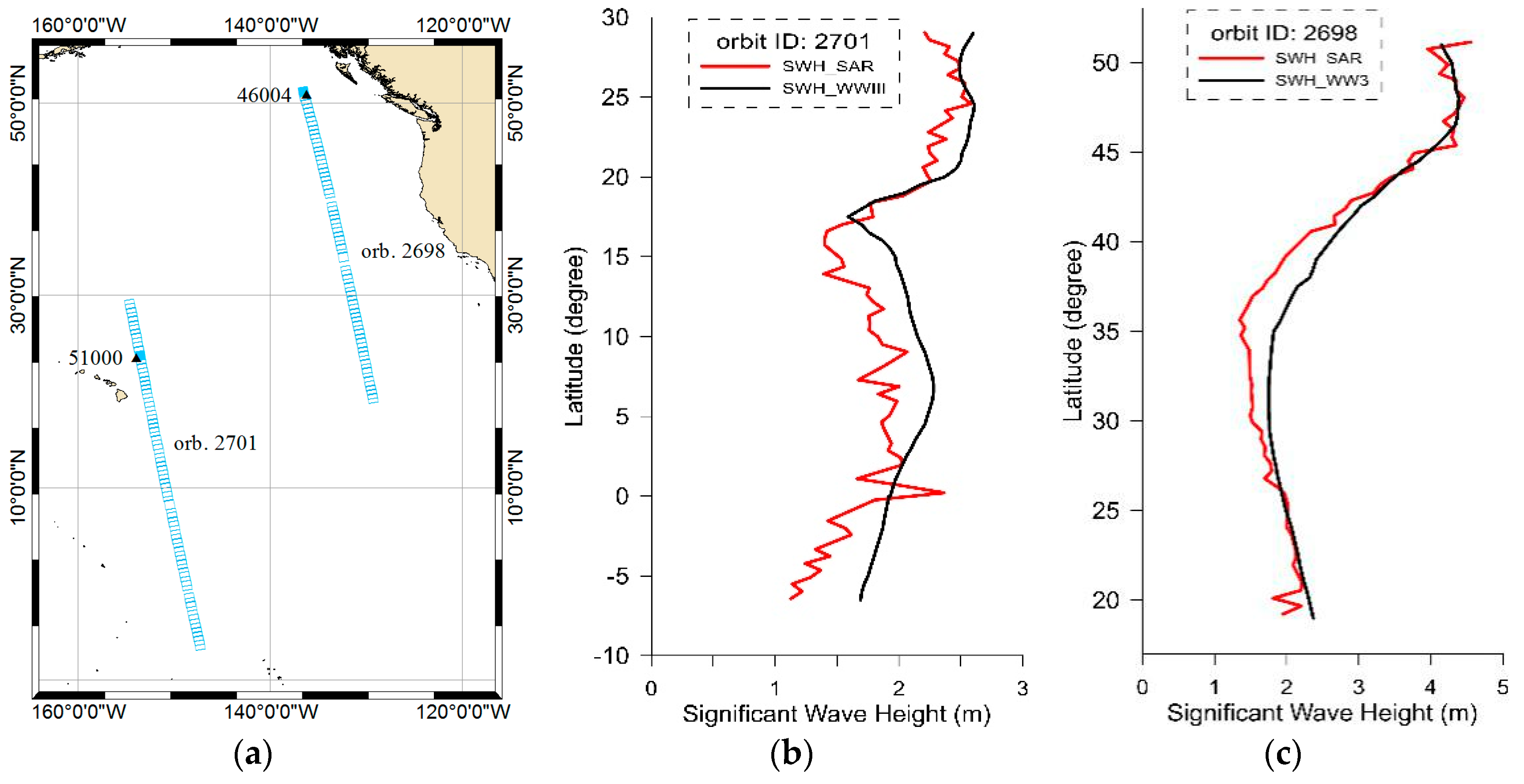
Figure 8a shows geolocations of GF-3 wave mode data acquired from two orbits on February 13, 2017 off the western coast of the United States. The locations of buoys 46004 and 51000 are marked with triangles. The SAR-retrieved SWH from these wave mode data were compared with the wave watch III (WW3) model results (available from http://polar.ncep.noaa.gov/waves/ensemble/download.shtml), as presented in Figure 8b, c for the two orbits. The sea state covering the area for the orbit 2701 was slightly low (less than 2.5 m), while that for 2698 was relatively rough (higher than 2.5 m). In general, the SAR retrievals are consistent with the WW3 model results, but they also pre-sent spatial sea state variations, particularly in the sea over which orbit 2701 passed.
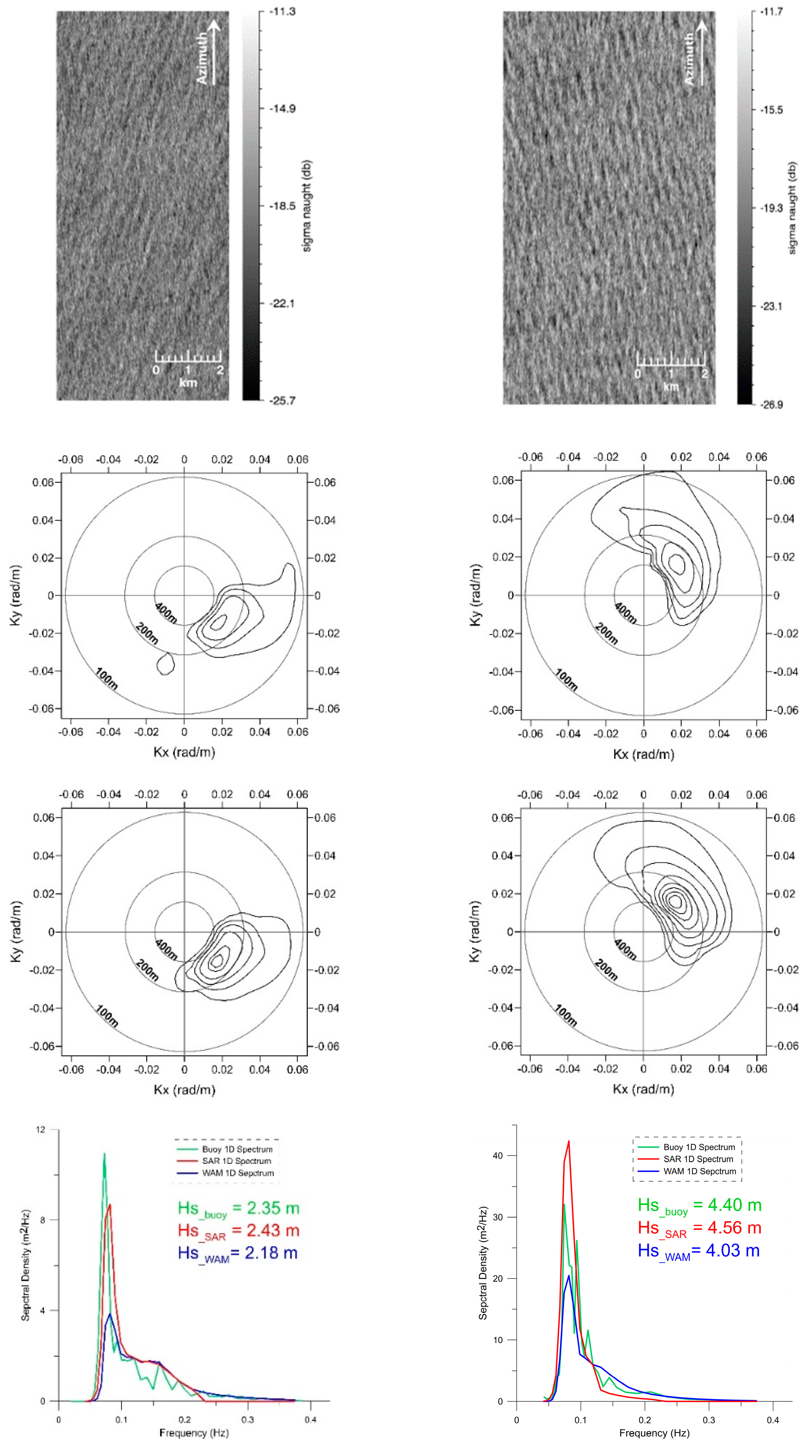
Figure 9 shows the two GF-3 wave mode imagettes near the two buoys and their corresponding retrievals. Both imagettes present clear swell patterns (the first row in Figure 9). The WAM model spectra (the second row) in the closest grid to the SAR acquisitions suggest that the swell propagated southeast and northwest, respectively, in the sea where the two images were acquired. The retrieval processes did not change much of the model spectra shapes, i.e., the first guess spectra, as found in the retrieved two-dimensional wave spectra (the third row). However, the retrieval did change the swell peak wave energy in the comparisons of one-dimensional wave spectra (the fourth row). Thus, the retrieved SWH is closer than the wave model to the buoy measurements. Interestingly, the two retrieved wave spectra indicate two different swell systems, although their peak wavelengths are almost identical. With respect to the retrieval of the GF-3 wave mode imagettes near buoy 51000, we deduce these swells came from North Pacific storms, whereas for the other image, which was nearer to the U.S. west coast, the swells likely came from the Southern Ocean, even though orbit 2698 is around two thousand kilometers east of orbit 2701.
5. Summary and Conclusions
In this study, we provided an overall assessment of the GF-3 SAR’s capability for selected ocean and coastal observation. To study radar backscatter mechanisms of complicated objects, specifically seaweed aquaculture in the Subei Shoal, polarization decomposition based on GF-3 QPS data appropriately reflects the dominant scattering mechanisms of aquaculture areas. To demonstrate the high spatial resolution of GF-3, we investigated the Donghai Bridge offshore wind farm, which highlighted the capability of GF-3 data to observe the tidal current wake rather than the wind wakes generated by the rotating wind turbines. Tidal current wakes have a smaller spatial scale of hundreds of meters than wind turbine wakes of tens of kilometers, and we previously used a high spatial resolution TSX image to identify this type of fine feature. Notably, the GF-3 image of the Donghai Bridge area clearly showed similar tidal current wakes. Finally, IWs are mesoscale phenomena that often have long wave crests exceeding a few hundred kilometers in the SCS, appearing in wave packets separated with varying distances. Therefore, it is preferable to use wide-swath SAR images for IWs. The case study of two GF-3 narrow ScanSAR images acquired in Dongsha Atoll demonstrated that the ScanSAR images could differentiate ISW refraction and diffraction around Dongsha Atoll and suggested variations in different wave packets arriving at Dongsha Atoll in one tidal cycle. However, the ScanSAR images manifested inhomogeneities in radar backscatter from beam to beam. Although this feature is rare, care should still be taken with the data processing system. We also noticed that the scalloping effect exists in some ScanSAR and Wide ScanSAR images of GF-3, particularly in the cross-polarization channels. De-scalloping should be undertaken during postprocessing (e.g., presented in [32]) for quantitative retrieval of marine-meteorological parameters.
Following these case studies, we investigated the capabilities of GF-3 QPS data for sea surface wind retrieval. A major conclusion of this investigation is that the recently provided calibration constants for the quad-polarization data significantly improve sea surface wind retrieval, with a bias of −0.15 m/s and an RMSE of 1.72 m/s, for wind speeds ranging from 2 m/s to 16 m/s. While the results were very close to the retrieved wind speed using the derived calibration constants in this study, they suggest that there is room to improve the GF-3 radiometric calibration accuracy. We also derived a linear function to derive sea surface wind speed from the GF-3 VH polarization data. The collection of more data will allow further investigation of the weak dependence of on incidence angles, as well as its performance in retrieving high wind speeds. Nevertheless, with the current data, we can derive SSW from both VV and VH polarization data in a consistent manner.
In addition to the ESA’s SAR mission, the Chinese GF-3 can also acquire wave mode data, albeit only in some regions thus far due to the limited coverage of the ground receiving stations. Nevertheless, our preliminary studies on the wave mode retrieval of two-dimensional wave spectra using nonlinear inversion demonstrate the usefulness of GF-3 for wave measurements. We expect that more wave mode data will be acquired and anticipate joint measurements with Sentinel-1A/1B wave mode data. In addition, the GF-3 wave mode data are acquired in full polarimetry and might provide a good opportunity to derive ocean wave information in a polarimetric manner [56].
Although we have presented a few informative examples, further detailed and dedicated efforts are needed to examine and improve data quality, considering that GF-3 has 12 available imaging modes and various polarization combinations. For instance, accurate radiometric calibration and noise estimation are particularly important for deriving the marine-meteorological parameters of sea surface wind and wave. Furthermore, stable performance is also important for an operational SAR data processing system. As more GF-3 data are acquired and analyzed, some abnormalities have been identified. The reasons underlying the occurrence of these cases should be investigated, and reprocessing of these data should be conducted.
Author Contributions
Conceptualization, X.-M.L.; methodology, X.-M.L.; formal analysis, all authors; investigation, all authors; resources, X.-M.L.; data curation, T.Z., B.H., and T.J.; original draft preparation, all authors; writing—review and editing, X.-M.L.; visualization, all authors; supervision, X.-M.L.; project administration, X.-M.L.; funding acquisition, X.-M.L.
Funding
This research was funded by the National Key Research and Development Program of China (2018YFC1407100), the National Natural Science Foundation of China (grant no. 41471309) and the National High-Resolution Project of China (grant no. Y20A14-9001-15/16).
Acknowledgments
It is acknowledged that the GF-3 SAR data were acquired from the ground segment of the Institute of Remote Sensing and Digital Earth, CAS and data portal of National Satellite Ocean Application Service (NSOAS). We specifically thank the ECMWF, NOAA NDBC and NCEP, and Remote Sensing Systems for providing the comparison datasets. The webpages where these data can be accessed are listed in the text.
Conflicts of Interest
The authors declare no conflict of interest.
References
- Vesecky, J.F.; Stewart, R.H. The observation of ocean surface phenomena using imagery from the SEASAT synthetic aperture radar: An assessment. J. Geophys. Res. 1982, 87, 3397–3430. [Google Scholar] [CrossRef]
- Liu, A.K.; Hsu, M.K. Internal wave study in the South China Sea using Synthetic Aperture Radar (SAR). Int. J. Remote Sens. 2004, 25, 1261–1264. [Google Scholar] [CrossRef]
- Li, X.F.; Dong, C.P.; Clemente-Colon, P.; Pichel, W.G.; Friedman, K.S. Synthetic aperture radar observations of sea surface imprints of upstream atmospheric solitons generated by flow impeded by an island. J. Geophys. Res. 2004, 109, C02016. [Google Scholar] [CrossRef]
- Reppucci, A.; Lehner, S.; Schulz-Stellenfleth, J.; Brusch, S. Tropical Cyclone Intensity Estimated from Wide-Swath SAR Images. IEEE Trans. Geosci. Remote Sens. 2010, 48, 1639–1649. [Google Scholar] [CrossRef]
- Chapron, B.; Collard, F.; Ardhuin, F. Direct measurements of ocean surface velocity from space: Interpretation and validation. J. Geophys. Res. 2005, 110, C07008. [Google Scholar] [CrossRef]
- Morena, L.C.; James, K.V.; Beck, J. An introduction to the RADARSAT-2 mission. Can. J. Remote Sens. 2004, 30, 221–234. [Google Scholar] [CrossRef]
- Buckreuss, S.; Werninghaus, R.; Pitz, W. The German satellite mission TerraSAR-X. In Proceedings of the IEEE Radar Conference, Rome, Italy, 26–30 May 2008; pp. 1–5. [Google Scholar]
- Covello, F.; Battazza, F.; Coletta, A.; Manoni, G.; Valentini, G. COSMO-SkyMed mission status: Three out of four satellites in orbit. In Proceedings of the IEEE International Geoscience and Remote Sensing Symposium (IGARSS), Cape Town, South Africa, 12–17 July 2009; pp. II-773–II-776. [Google Scholar]
- Brusch, S.; Lehner, S.; Fritz, T.; Soccorsi, M.; Soloviev, A.; Schie, V.B. Ship Surveillance with TerraSAR-X. IEEE Trans. Geosci. Remote Sens. 2011, 49, 1092–1103. [Google Scholar] [CrossRef]
- Pastina, D.; Fico, F.; Lombardo, P. Detection of ship targets in COSMO-SkyMed SAR images. In Proceedings of the IEEE RadarCon (RADAR), Kansas City, MO, USA, 23–27 May 2011; pp. 928–933. [Google Scholar]
- Vachon, P.W.; Kabatoff, C.; Quinn, R. Operational ship detection in Canada using RADARSAT. In Proceedings of the IEEE International Geoscience and Remote Sensing Symposium (IGARSS), Quebec City, QC, Canada, 13–18 July 2014; pp. 998–1001. [Google Scholar]
- Velotto, D.; Migliaccio, M.; Nunziata, F.; Lehner, S. Dual-polarized TerraSAR-X data for oil-spill observation. IEEE Trans. Geosci. Remote Sens. 2011, 49, 4751–4762. [Google Scholar] [CrossRef]
- Zhang, B.; Perrie, W.; Li, X.F.; Pichel, W.G. Mapping sea surface oil slicks using RADARSAT-2 quad-polarization SAR image. Geophys. Res. Lett. 2011, 38, L10602. [Google Scholar] [CrossRef]
- Migliaccio, M.; Nunziata, F.; Brown, C.E.; Holt, B.; Li, X.F.; Pichel, W.G.; Shimada, M. Polarimetric synthetic aperture radar utilized to track oil spills. Trans. EOS 2012, 93, 161–163. [Google Scholar] [CrossRef]
- Choe, B.H.; Kim, D.J.; Hwang, J.H.; Oh, Y.; Moon, W.M. Detection of oyster habitat in tidal flats using multi-frequency polarimetric SAR data. Estuar. Coast. Shelf Sci. 2012, 97, 28–37. [Google Scholar] [CrossRef]
- Geng, X.M.; Li, X.M.; Velotto, D.; Chen, K.S. Study of the polarimetric characteristics of mud flats in an intertidal zone using C- and X-band spaceborne SAR data. Remote Sens. Environ. 2016, 176, 56–68. [Google Scholar] [CrossRef]
- Gade, M.; Wang, W.S.; Kemme, L. On the imaging of exposed intertidal flats by single- and dual-co-polarization Synthetic Aperture Radar. Remote Sens. Environ. 2018, 205, 315–328. [Google Scholar] [CrossRef]
- Dierking, W.; Wesche, C. C-Band Radar Polarimetry is Useful for Detection of Icebergs in Sea Ice? IEEE Trans. Geosci. Remote Sens. 2014, 52, 25–37. [Google Scholar] [CrossRef]
- Ressel, R.; Singha, S.; Lehner, S.; Rösel, A.; Spreen, G. Investigation into Different Polarimetric Features for Sea Ice Classification Using X-Band Synthetic Aperture Radar. IEEE J. Sel. Top. Appl. Earth Observ. Remote Sens. 2016, 9, 3131–3143. [Google Scholar] [CrossRef] [Green Version]
- Johansson, M.A.; Brekke, C.; Spreen, G.; King, J.A. X-, C-, and L-band SAR signatures of newly formed sea ice in Arctic leads during winter and spring. Remote Sens. Environ. 2018, 204, 162–180. [Google Scholar] [CrossRef]
- Ciappa, A.; Pietranera, L.; Coletta, A.; Jiang, X.W. Surface transport detected by pairs of COSMO-SkyMed ScanSAR images in the Qingdao region (Yellow Sea) during a macro-algal bloom in July 2008. J. Marine Syst. 2010, 80, 135–142. [Google Scholar] [CrossRef]
- Cheng, Y.; Liu, B.; Li, X.; Nuziata, F.; Xu, Q.; Ding, X.; Migliaccio, M.; Pichel, W.G. Monitoring of Oil Spill Trajectories With COSMO-SkyMed X-Band SAR Images and Model Simulation. IEEE Trans. Geosci. Remote Sens. 2014, 7, 2895–2901. [Google Scholar] [CrossRef]
- Ren, Y.; Li, X.M.; Gao, G.; Busche, T.E. Derivation of Sea Surface Tidal Current from Spaceborne SAR Constellation Data. IEEE Trans. Geosci. Remote Sens. 2017, 55, 3236–3247. [Google Scholar] [CrossRef]
- Romeiser, R.; Suchandt, S.; Runge, H.; Steinbrecher, U.; Grunler, S. First Analysis of TerraSAR-X Along-Track InSAR-Derived Current Fields. IEEE Trans. Geosci. Remote Sens. 2010, 48, 820–829. [Google Scholar] [CrossRef]
- Kerbaol, V.; Chapron, B.; Vachon, P.W. Analysis of ERS-1/2 synthetic aperture radar wave mode imagettes. J. Geophys. Res. 1998, 103, 7833–7846. [Google Scholar] [CrossRef] [Green Version]
- Lehner, S.; Schulz-Stellenfleth, J.; Schattler, B.; Breit, H.; Horstmann, J. Wind and wave measurements using complex ERS-2 SAR wave mode data. IEEE Trans. Geosci. Remote Sens. 2000, 38, 2246–2257. [Google Scholar] [CrossRef]
- Schulz-Stellenfleth, J.; Lehner, S.; Hoja, D. A parametric scheme for the retrieval of two-dimensional ocean wave spectra from synthetic aperture radar look cross spectra. J. Geophys. Res. 2005, 110, C05004. [Google Scholar] [CrossRef]
- Schulz-Stellenfleth, J.; König, T.; Lehner, S. An empirical approach for the retrieval of integral ocean wave parameters from synthetic aperture radar data. J. Geophys. Res. 2007, 112, C03019. [Google Scholar] [CrossRef]
- Li, X.M. A new insight from space into swell propagation and crossing in the global oceans. Geophys. Res. Lett. 2016, 43, 5202–5209. [Google Scholar] [CrossRef]
- Stopa, J.E.; Mouche, A. Significant wave heights from Sentinel-1 SAR: Validation and applications. J. Geophys. Res. Oceans. 2017, 122, 1827–1848. [Google Scholar] [CrossRef]
- De Zan, F.; Guarnieri, A.M. TOPSAR: Terrain Observation by Progressive Scans. IEEE Trans. Geosci. Remote Sens. 2006, 44, 2352–2360. [Google Scholar] [CrossRef]
- Romeiser, R.; Horstmann, J.; Caruso, M.J.; Graber, H.C. A Descalloping Postprocessor for ScanSAR Images of Ocean Scenes. IEEE Trans. Geosci. Remote Sens. 2013, 51, 3259–3272. [Google Scholar] [CrossRef]
- Wang, H.; Yang, J.S.; Mouche, A.; Shao, W.Z.; Zhu, J.H.; Ren, L.; Xie, C.H. GF-3 SAR ocean wind retrieval: The first view and preliminary assessment. Remote Sens. 2017, 9, 694. [Google Scholar] [CrossRef]
- Ren, L.; Yang, J.S.; Mouche, A.; Wang, H.; Wang, J.; Zheng, G.; Zhang, H.G. Preliminary Analysis of Chinese GF-3 SAR Quad-Polarization Measurements to Extract Winds in Each Polarization. Remote Sens. 2017, 9, 1215. [Google Scholar] [CrossRef]
- Wang, H.; Wang, J.; Yang, J.S.; Ren, L.; Zhu, J.H.; Yuan, X.Z.; Xie, C.H. Empirical Algorithm for Significant Wave Height Retrieval from Wave Mode Data Provided by the Chinese Satellite Gaofen-3. Remote Sens. 2018, 10, 363. [Google Scholar] [CrossRef]
- Shao, W.Z.; Sheng, Y.X.; Sun, J. Preliminary Assessment of Wind and Wave Retrieval from Chinese Gaofen-3 SAR Imagery. Sensors 2017, 17, 1705. [Google Scholar] [CrossRef] [PubMed]
- Sato, A.; Yamaguchi, Y.; Singh, G.; Park, S.E. Four-component scattering power decomposition with extended volume scattering model. IEEE Geosci. Remote Sens. Lett. 2012, 9, 166–170. [Google Scholar] [CrossRef]
- Li, Y.; Xiao, J.; Ding, L.; Wang, Z.; Song, W.; Fang, S.; Fan, S.; Li, R.; Zhang, X. Community structure and controlled factor of attached green algae on the Porphyra yezoensis aquaculture rafts in the Subei Shoal, China. Acta Oceanol. Sin. 2015, 34, 93–99. [Google Scholar] [CrossRef]
- Zhou, M.J.; Liu, D.Y.; Anderson, D.M.; Valiela, I. Introduction to the Special Issue on green tides in the Yellow Sea. Estuar. Coast. Shelf Sci. 2015, 163, 3–8. [Google Scholar] [CrossRef] [Green Version]
- Schneiderhan, T.; Lehner, S.; Schulz-Stellenfleth, J.; Horstmann, J. Comparison of offshore wind park sites using SAR wind measurement techniques. Meteorol. Appl. 2005, 12, 101–110. [Google Scholar] [CrossRef] [Green Version]
- Christiansen, M.B.; Hasager, C.B. Wake effects of large offshore wind farms identified from satellite SAR. Remote Sens. Environ. 2005, 98, 251–268. [Google Scholar] [CrossRef]
- Li, X.M.; Lehner, S. Observation of TerraSAR-X for Studies on Offshore Wind Turbine Wake in Near and Far Fields. IEEE J. Sel. Top. Appl. Earth Observ. Remote Sens. 2013, 6, 1757–1768. [Google Scholar] [CrossRef] [Green Version]
- Li, X.M.; Chi, L.Q.; Chen, X.E.; Ren, Y.Z.; Lehner, S. SAR observation and numerical modeling of tidal current wakes at the East China Sea offshore wind farm. J. Geophys. Res. 2014, 119, 4958–4971. [Google Scholar] [CrossRef] [Green Version]
- Vanhellemont, Q.; Ruddick, K. Turbid wakes associated with offshore wind turbines observed with Landsat 8. Remote Sens. Environ. 2014, 145, 105–115. [Google Scholar] [CrossRef]
- Grashorn, S.; Stanev, E.V. Kármán vortex and turbulent wake generation by wind park piles. Ocean Dyn. 2016, 66, 1543–1557. [Google Scholar] [CrossRef]
- Li, X.; Jackson, C.R.; Pichel, W.G. Internal solitary wave refraction at Dongsha Atoll, South China Sea. Geophys. Res. Lett. 2013, 40, 3128–3132. [Google Scholar] [CrossRef] [Green Version]
- Jia, T.; Liang, J.J.; Li, X.M.; Sha, J. SAR observation and numerical simulation of internal solitary wave refraction and reconnection behind the Dongsha Atoll. J. Geophys. Res. Oceans. 2017, 123, 74–89. [Google Scholar] [CrossRef]
- Alpers, W. Theory of radar imaging of internal waves. Nature 1985, 314, 245–247. [Google Scholar] [CrossRef]
- Li, X.; Zhao, Z.; Pichel, W.G. Internal solitary waves in the northwestern South China Sea inferred from satellite images. Geophys. Res. Lett. 2008, 35, 344–349. [Google Scholar] [CrossRef]
- Vachon, W.P.; Wolfe, J. C-Band Cross-Polarization Wind Speed Retrieval. IEEE Geosci. Remote Sens. Lett. 2011, 8, 456–459. [Google Scholar] [CrossRef]
- Zhang, B.; Perrie, W.; He, Y. Wind speed retrieval from RADARSAT-2 quad-polarisation images using a new polarisation ratio model. J. Geophys. Res. 2011, 116, C08008. [Google Scholar] [CrossRef]
- Zadelhoff, G.J.; Stoffelen, A.; Vachon, P.W.; Wolfe, J.; Horstmann, J.; Belmonte Rivas, M. Retrieving hurricane wind speeds using cross polarization C-band measurements. Atmos. Meas. Tech. 2014, 7, 437–449. [Google Scholar] [CrossRef]
- Mouche, A.; Chapron, B. Global C-band Envisat, RADARSAT-2 and Sentinel-1 SAR measurements in copolarization and cross-polarization. J. Geophys. Res. Oceans 2015, 120, 7195–7207. [Google Scholar] [CrossRef]
- Hasselmann, K.; Hasselmann, S. On the nonlinear mapping of an ocean wave spectrum into a synthetic aperture radar image spectrum and its inversion. J. Geophys. Res. 1991, 96, 10713–10729. [Google Scholar] [CrossRef]
- Hasselmann, S.; Brüning, C.; Hasselmann, K.; Heimbach, P. An improved algorithm for the retrieval of ocean wave spectra from synthetic aperture radar image spectra. J. Geophys. Res. 1996, 101, 16615–16629. [Google Scholar] [CrossRef]
- He, Y.; Shen, H.; Perrie, W. Remote sensing of ocean waves by polarimetric SAR. J. Atmos. Ocean. Tech. 2006, 23, 1768–1773. [Google Scholar] [CrossRef]
Figure 1.
(a) Radiometrically calibrated HV polarization channel of the GF-3 QPS data acquired on 5 October 2017, in an ascending orbit. (b) Photo of a single raft in the study area, adapted from [39]. (c) Top-view photo of aquaculture rafts taken in the GF-3 imaged area. (d) False-color composite image generated using the normalized four-component decomposition of the GF-3 QPS data.


Figure 2.
(a) A GF-3 FSI image in HH polarization acquired at 9:45 UTC on 15 February 2014, over the eastern Hangzhou Bay and Changjiang River estuary, in an ascending orbit. (b) The sub-image of (a) over the offshore wind farm, showing distinct tidal current wake patterns. (c) Variation of Normalized Radar Cross Section (NRCS) along a transect (marked by the red rectangle in (b)) through a tidal turbulent wake. The dashed line indicates recovery of the turbulent wake at approximately 1000 m downstream of the turbine.


Figure 3.
(a) A GF-3 narrow ScanSAR image acquired on 21 October 2017, in ascending orbit, over Dongsha Atoll showing ISW signatures (left panel), the sub-image encompassing part of the ISWs in the southern Dongsha Atoll (upper right panel) and variations in the gray values of the transect corresponding to the red line in the sub-image (lower-right panel). (b) The same as (a) but for the image acquired on 24 October 2017, in a descending orbit.


Figure 4.
Distribution of ∆σ for different incidence angles of the GF-3 QPS mode data acquired from September 2016 to November 2017. The whiskers (red) are calculated from the samples of ∆σ. The upper extreme of each whisker is equal to Q3 + 1.5*IQR, where the IQR is the interquartile range of the samples (i.e., Q3–Q1) and the lower extreme is equal to Q1 − 1.5 × IQR.

Figure 5.
Retrieval of sea surface wind speed from the GF-3 QPS mode data in VV polarization using (a) the old calibration constant, (b) the new calibration constant released in May 2018, and (c) the revised calibration constants derived in this study.
Figure 5.
Retrieval of sea surface wind speed from the GF-3 QPS mode data in VV polarization using (a) the old calibration constant, (b) the new calibration constant released in May 2018, and (c) the revised calibration constants derived in this study.

Figure 6.
(a) Scatter plot of the GF-3 QPS values and the collocated ERA-Interim SSW. Boxes and whiskers, as well as linear fitting line are overlaid on the plot. (b) Comparison of the sea surface wind speed retrieval from GF-3 quad-polarization VH polarized data using Equation (9) with the collocated WindSat SSW speed data.

Figure 7.
(a) Comparison of the sea surface wind speeds derived from the VV and VH polarized data of GF-3 QPS data. (b) Example sea surface wind speed maps derived from both the VV (left) and VH (right) polarized data of QPS data acquired on 21 August 2017. The overlaid wind vectors are from the collocated WindSat data.

Figure 8.
(a) Geolocation of GF-3 wave mode data in orbits 2701 and 2698 on 13 February 2017 (blue squares) and the locations of buoys 51000 and 46004 (black triangles). (b) SAR-retrieved SWH (red line) from the wave mode data of orbit 2701 and the collocated WW3 SWH (black line). (c) The same as (b) but for the wave mode data of the orbit 2698.

Figure 9.
Two retrieval examples of the GF-3 wave mode data from orbit 2701 (left column) and orbit 2698 (right column). The SAR imagettes are in the first row. The collocated WAM spectra and the retrieved two-dimensional spectra are in the second and the third row, respectively. The one-dimensional spectra are compared in the last row.


Table 1.
Available GF-3 imaging modes and the corresponding technical specifications.
| No. | Imaging Mode | Incidence Angle (°) | Nominal Resolution (m) | Swath Width (km) |
|---|---|---|---|---|
| 1 | Spotlight Mode | 20–50 | 1 | 10 × 10 |
| 2 | Stripmap Mode | |||
| Superfine | 20–50 | 3 | 30 | |
| Fine | 19–50 | 5 | 50 | |
| Wide Fine | 19–50 | 10 | 100 | |
| Standard | 17–50 | 25 | 130 | |
| Quad-pol. 1 | 20–41 | 8 | 30 | |
| Quad-pol. 2 | 20–38 | 25 | 40 | |
| 3 | ScanSAR Mode | |||
| Narrow | 17–50 | 50 | 300 | |
| Wide | 17–50 | 100 | 500 | |
| Global | 17–53 | 500 | 650 | |
| 4 | Wave Mode | 20–41 | 10 | 5 × 5 |
© 2018 by the authors. Licensee MDPI, Basel, Switzerland. This article is an open access article distributed under the terms and conditions of the Creative Commons Attribution (CC BY) license (http://creativecommons.org/licenses/by/4.0/).
Share and Cite
MDPI and ACS Style
Li, X.-M.; Zhang, T.; Huang, B.; Jia, T. Capabilities of Chinese Gaofen-3 Synthetic Aperture Radar in Selected Topics for Coastal and Ocean Observations. Remote Sens. 2018, 10, 1929. https://doi.org/10.3390/rs10121929
AMA Style
Li X-M, Zhang T, Huang B, Jia T. Capabilities of Chinese Gaofen-3 Synthetic Aperture Radar in Selected Topics for Coastal and Ocean Observations. Remote Sensing. 2018; 10(12):1929. https://doi.org/10.3390/rs10121929
Chicago/Turabian StyleLi, Xiao-Ming, Tianyu Zhang, Bingqing Huang, and Tong Jia. 2018. "Capabilities of Chinese Gaofen-3 Synthetic Aperture Radar in Selected Topics for Coastal and Ocean Observations" Remote Sensing 10, no. 12: 1929. https://doi.org/10.3390/rs10121929
Note that from the first issue of 2016, this journal uses article numbers instead of page numbers. See further details here.