End-to-End Simulation of WCOM IMI Sea Surface Salinity Retrieval


1
Key Laboratory of Microwave Remote Sensing, National Space Science Center, Chinese Academy of Sciences, Beijing 100190, China
2
University of Chinese Academy of Sciences, Beijing 100094, China
*
Author to whom correspondence should be addressed.
Remote Sens. 2019, 11(3), 217; https://doi.org/10.3390/rs11030217
Submission received: 29 November 2018
/
Revised: 10 January 2019
/
Accepted: 17 January 2019
/
Published: 22 January 2019
(This article belongs to the Special Issue Sea Surface Salinity Remote Sensing)
Abstract
:The Water Cycle Observation Mission (WCOM) is an Earth science mission focused on the observation of the water cycle global climate change intensity through three different payloads. WCOM’s main payload is an interferometric microwave imager (IMI). IMI is a tri-frequency, one-dimensional aperture synthesis microwave radiometer operating at the L-, S-, and C-bands to perform measurements of soil moisture and ocean salinity. Focusing on sea surface salinity (SSS), an end-to-end simulator of WCOM/IMI has been realized and tested on climatological data. Results indicate a general agreement between original and retrieved SSS, with a single measurement root mean square error of 0.26 psu and with an orbital measurement of 0.17 psu in open sea. In accordance with previous studies, good results are obtained in open sea, while strong contamination is observed in coastal areas.
1. Introduction
The Chinese Water Cycle Observation Mission (WCOM), subject to the Strategic Space Science Priority Project of the Chinese Academy of Sciences, is planned to be launched in the near future. The WCOM aims to observe and track the main parameters related to the global water cycle, including soil moisture, ocean salinity, snow water equivalent, soil freeze-thaw, atmospheric water vapor, and precipitation [1].
To achieve the goals above, the WCOM relies on the following three payloads: (1) An interferometric microwave imager (IMI), a tri-frequency one-dimensional (1D) interferometric microwave radiometer operating at the L-, S-, and C-bands to measure soil moisture and sea surface salinity; (2) a polarimetric microwave imager (PMI), a conically scanning polarimetric radiometer operating at multiple frequencies between the C- and the W-band, with full polarimetric capabilities for most of them (it aims to measure land and sea surface temperature, water vapor, and precipitation); and (3) a dual-frequency polarized SCATterometer (DFPSCAT) to measure the snow water equivalent and soil freeze–thaw [2].
L-band microwave radiometry has been widely agreed as the most effective tool to measure soil moisture and ocean salinity from space. In fact, three satellite missions embarking with L-band radiometers have been launched in the past decade, namely ESA’s Soil Moisture and Ocean Salinity mission (SMOS) [3], NASA’s Aquarius/SAC-D [4], and Soil Moisture Active/Passive mission (SMAP) [5]. However, the retrieval of salinity is still considered challenging due to the low sensitivity of brightness temperature (TB) to salinity (from 0.8 K down to 0.2 K per psu, depending on ocean surface temperature, radiometer incidence angle, and polarization [6]), making it hard to meet the accuracy and stability requirements for application and research.
This study focuses on the analysis of sea surface salinity (SSS) using the tri-frequency 1D aperture synthesis radiometer IMI onboard the WCOM satellite, and is structured as follows. Section 2 provides an introduction on the instrument and methods applied in the end-to-end simulation. This is followed by the simulation results, including TB reconstruction and salinity retrieval, which are presented and discussed in Section 3. Finally, the main conclusions are summarized in Section 4.
2. Concepts and Methods
2.1. Interferometric Microwave Imager (IMI)
The system performance characteristics for the WCOM/IMI are listed in Table 1.
Like SMOS’s MIRAS, IMI adopts aperture synthesis technology to overcome the barrier that the antenna size places at the L-band. Specifically, IMI is a tri-frequency (L-, S-, and C-bands) 1D interferometric radiometer consisting of a deployable 6 m parabolic cylinder mesh reflector and a tri-frequency patch feed array. Additionally, as a 1D interferometric radiometer, IMI has a lower system complexity compared with the two-dimensional MIRAS, indicating that it is much easier to control its in-orbit instrument stability and calibration accuracy.
As mentioned above, besides the L-band, the IMI also operates at the S- and C-bands, which can improve its sensitivity to soil moisture on land and assist in taking measurements of SSS and sea surface temperature (SST) on the ocean.
2.2. End-to-End Simulation Model and Method
The end-to-end simulation for ocean salinity in this paper is based on previous work regarding the 1D interferometric radiometer IMI simulation system [7], the sea radiometer transfer model, and a salinity retrieval algorithm. The simulation system is built on the Matlab platform.
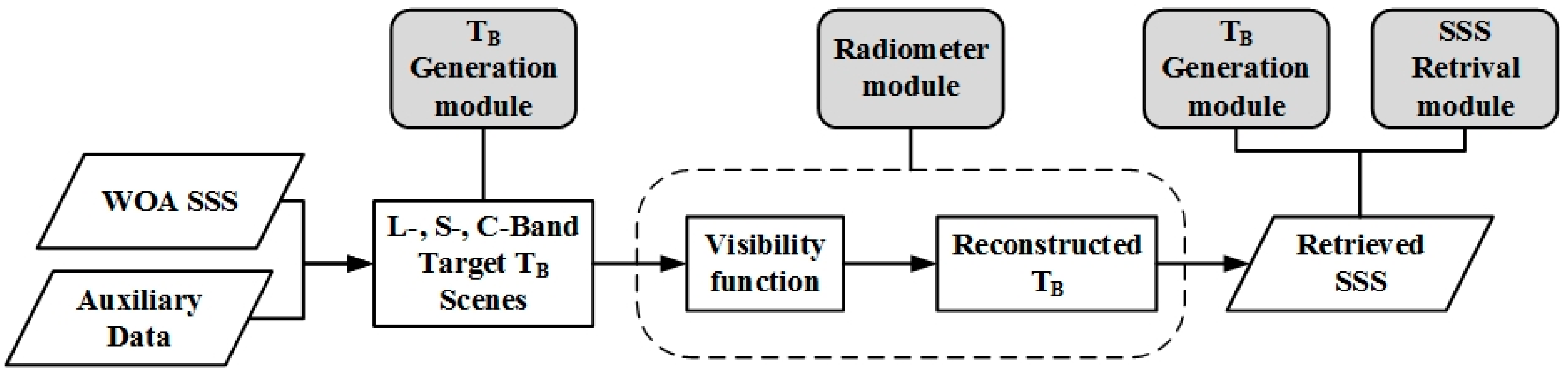
The end-to-end simulation flow is shown in Figure 1. It begins with the input salinity data and ends with the retrieved SSS from the simulated “measured” TB. In the simulation, the original SSS, together with auxiliary data, were processed into the target TB scenes in different bands. These then formed the visibility function through the radiometer simulation. Afterwards, the visibility function was again reconstructed into TB. Finally, the retrieved SSS were achieved through the comparison between the reconstructed TB and the modeled TB. The modules used in the end-to-end simulation chain are highlighted as grey cases at the top of Figure 1.
2.2.1. TB Generation Module
As seen from Figure 1, the TB generation module was used not only in the measurement scene generation as an input to the radiometer module, but also in the SSS retrieval module to calculate and update the modeled TB.
According to [8], the TB at the top of the atmosphere in the Earth reference frame can be calculated using Equation (1).
where is the TB radiated by the ocean surface and can be further calculated using Equation (2).
where is described as the sum of TB in the case of a flat sea () and additional TB due to surface roughness (). is the emission of a flat sea surface, which can be described as a function of the SST and the Fresnel reflectivity. , which in turns depends on the incident angle () and the complex dielectric constant of sea water (). In this paper, is calculated using the Klein–Swift model [9] for the L- and S-band and the Meissner–Wentz model [10] for the C-band. For a rough sea surface, is computed with a two-scale model [11] for the L- and S-band and is computed with the model from AMSR-E [12] for the C-band.
In Equation (1), and refer to the downward and upward atmospheric radiation, respectively, is the atmospheric opacity, and is the optical thickness. The model used for the atmosphere is from the ESA’s SMOS mission for the L-band and from AMSR-E [12] for the C-band. Finally, is the sea surface reflection coefficient, which can be expressed as , and is the cosmic and galactic contribution.
After the calculation of TB in the Earth reference frame, the TB in the antenna reference frame is obtained through multiplying the polarization rotation matrix as shown below.
where, , , and are the antenna TB, is the angle of polarization rotation, and are the horizontal and vertical components of TB in the Earth’s reference frame, respectively.
2.2.2. Radiometer Module
In Figure 1, the radiometer simulation module processes the “measured” TB calculated from the TB generation module into the visibility function using the model of radiometer system. The visibility function calculation is described considering the weighted function of the antenna pattern [13,14], by applying Equation (4).
where is the normalized antenna pattern, which is a complex function including amplitude and phase; is the TB from the observation scene; is the fringe-washing function, which accounts for spatial decorrelation effects and depends on the frequency response of the pair of elements collecting the signals being correlated; and and are the direction cosine coordinates (, , with and being the angle in the instrument plane and the angle from the normal to the instrument plane, respectively. For IMI, a 1D radiometer, in Equation (4).
Equation (4) is the ideal equation for the visibility function of interferometric synthetic aperture radiometers. To include the image errors introduced by coupling effects between the antennas, in Equation (4) is replaced by , where is the physical temperature of the receivers and assumed to be 300 K in the simulation. This leads to the formulation of the Corbella equation.
The resulting are processed by the TB reconstruction for generating the “measured” TB. Due to the difference between antenna patterns described in Section 2.3, it is not proper to directly apply the Fourier-based image reconstruction method. Specifically, the G matrix method [15,16] is used to reconstruct the TB map as, expressed in Equation (5).
where is the reconstructed TB, is the pseudoinverse matrix of the G matrix, and subscript i indicates the i-th visibility sample. There are only 18 continuous, non-redundant visibility samples for the eight-element linear feed array, forming a small-sized G matrix, simplifying the calculation of the pseudo-inverse through the Moor-Penrose method, and thus the image reconstruction.
2.2.3. SSS Retrieval Module
The SSS retrieval is based on a nonlinear iterative convergence algorithm where the prior values of the parameters to be retrieved were adjusted in order to minimize a cost function [16]. TB values were calculated by applying the TB generation module described in Section 2.2.1 and were compared to the “measured” TB resulting from the radiometer simulation module.
The L- and S-band-measured TB data were suitable to retrieve SSS, while the C-band measured TB was used as auxiliary data to assist in the retrieval of SSS, and to retrieve SST. Thus, the cost function based on all the data of the three bands is expressed as
where, , , and indicate the “measured” TB at different bands (L-, S-, and C-band, respectively) and polarizations (horizontal and vertical), and , and , are the corresponding uncertainties. Lastly, and refer to the prior estimated values for SSS and SST associated with the corresponding uncertainties and . Since the current study focuses on salinity retrieval, the retrieval results of SST are not included.
2.3. Simulation Input
For IMI instrument concept proofing and performance validation, a ground-based demonstrator designed with an eight-element L-band radiometer is developed in 2011 [2] and applied in several ground-based experiments targeting different objects, such as buildings, the sun, the cold sky, a noise point source, etc. A picture of the aforementioned IMI prototype and a schematic of the arrangement of the antenna units in the 1D feed array are shown in Figure 2a and Figure 2b, respectively. The scatterometer units involved in the 1D feed array make the prototype a combined active/passive instrument. Anyway, since the performance of the radiometer instrument is the focus of this paper, only the radiometer feed array is adopted in the simulation.
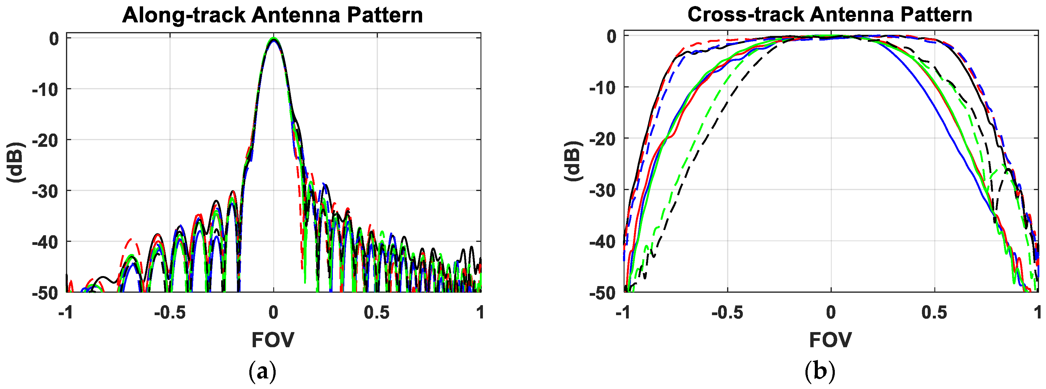
Both the actual measured antenna pattern and the distribution of the IMI prototype were applied in the simulation. Specifically, as seen in Figure 2b, the whole eight-element radiometer feed was considered a mixed array constituted by three small-size and five large-size antenna units, in which the minimum antenna spacing of the antenna array was 0.6125 λ. Along-track and cross-track antenna patterns measured from the prototype experiment for each unit are presented in Figure 3a and Figure 3b, respectively.
The alias-free field of view (AF-FOV) areas were calculated using and applying , leading to an observation angle included between −55° and 55°, approximately. All the reconstructed TB data within the AF-FOV were considered valid for the SSS retrieval.
Other simulation inputs include geophysical data and orbit parameters. The orbit is configured as a sun-synchronous orbit with an altitude of 657 km and inclination of 98°, and the local time of the ascending node is at 6:00 a.m. Geophysical data, including SST, 10-m wind speed, columnar atmospheric water vapor, and cloud liquid water were measured from AMSR-E [17], which are monthly averaged maps that all have spatial resolution of 0.25°. The original salinity map comes from World Ocean Atlas (WOA) 2013 [18], which is an in situ monthly averaged map with a spatial resolution of 1°. In order to be consistent in the simulation, the salinity map is interpolated into a 0.25° × 0.25° dimension.
Besides, the configuration of this simulation included both the measured antenna patterns and the image reconstruction error, and there was no additional noise or drift between the parameters used in the forward models and those used for the retrieval.
3. Results and Discussion
3.1. TB Reconstruction Results
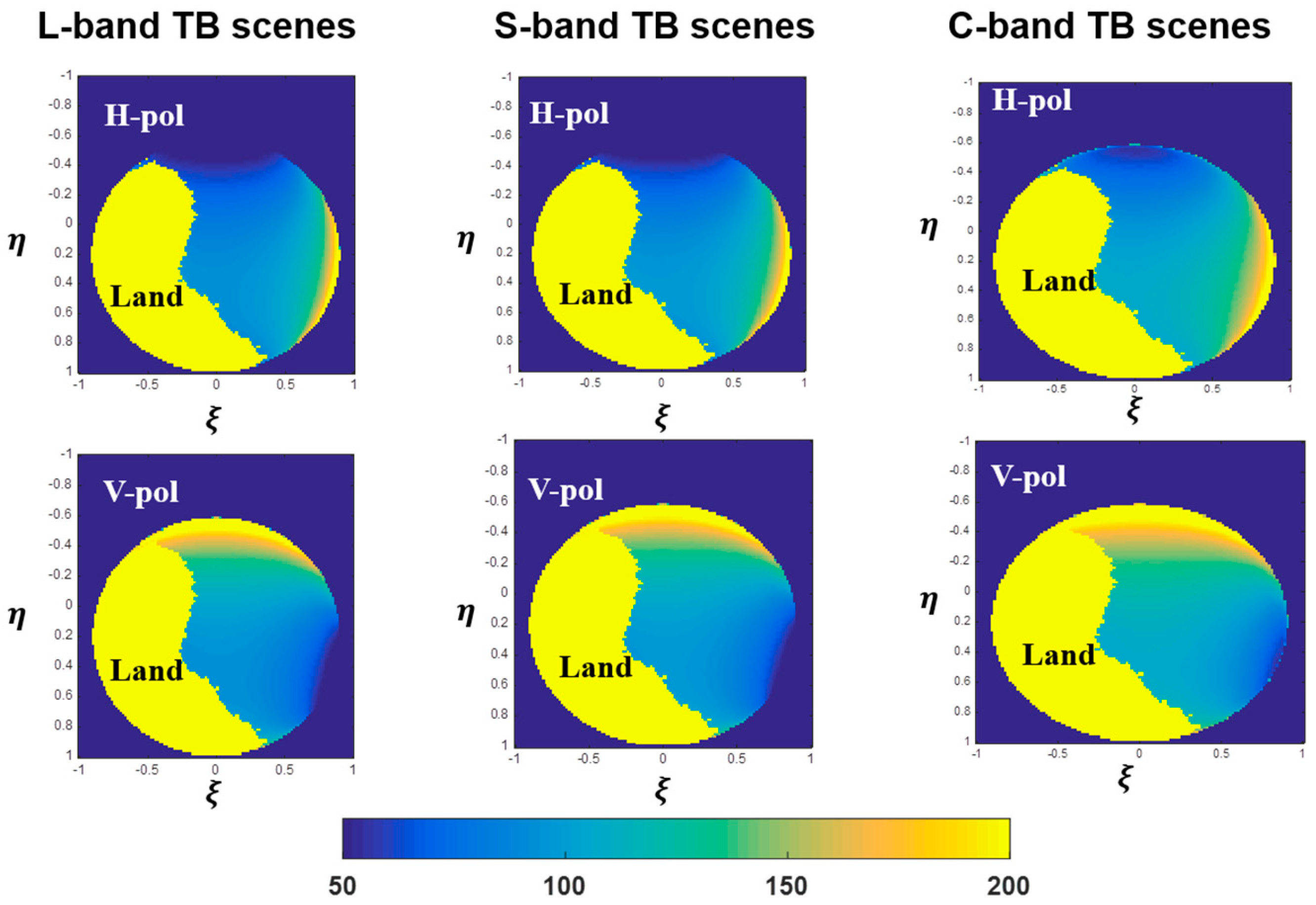
The specific scene obtained for a sub-satellite point located at 62.68 W, 13.78 N is shown in Figure 4. The results of the TB generation module at the L-, S-, and C-bands are displayed on the left, center, and right panels, respectively, with horizontal (H-pol) and vertical polarizations (V-pol) on the top and bottom rows, respectively.
The TB scenes in Figure 4 are used as inputs for the successive radiometer simulation to achieve TB reconstruction results. Due to the lack of measurement data from the S- and C-band antenna array, only TB reconstruction as a result of the L-band is presented in the following figure, similar results are expected at the other bands.
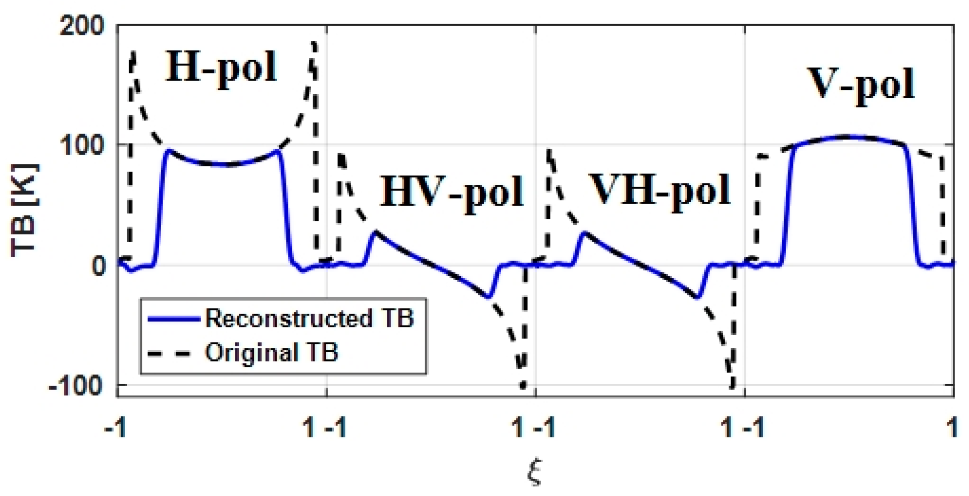
Since the antenna array of IMI is 1D, the output from the TB reconstruction of the radiometer module is also 1D. Results of all the measured polarizations are shown in Figure 5, with the reconstructed TB data represented by the blue solid line and the simulated TB represented by the black dashed line. Good agreement is found between modeled and retrieved TB in the AF-FOV areas, with a root mean square error (RMSE) of 0.09 K.
3.2. SSS Retrieval Results
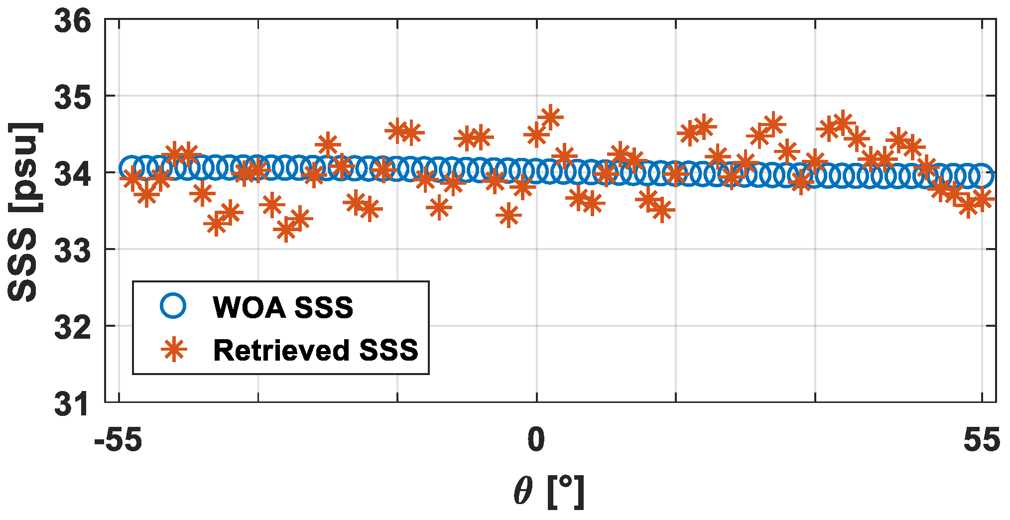
In Figure 6, the results of SSS retrieval from a single measurement are shown. The retrieved SSS from each measurement are mapped into Earth coordinates in order to compare them with the WOA salinity data. The differences between WOA SSS and retrieved SSS are generally within ±0.5 psu, with an RMSE of 0.26 psu.
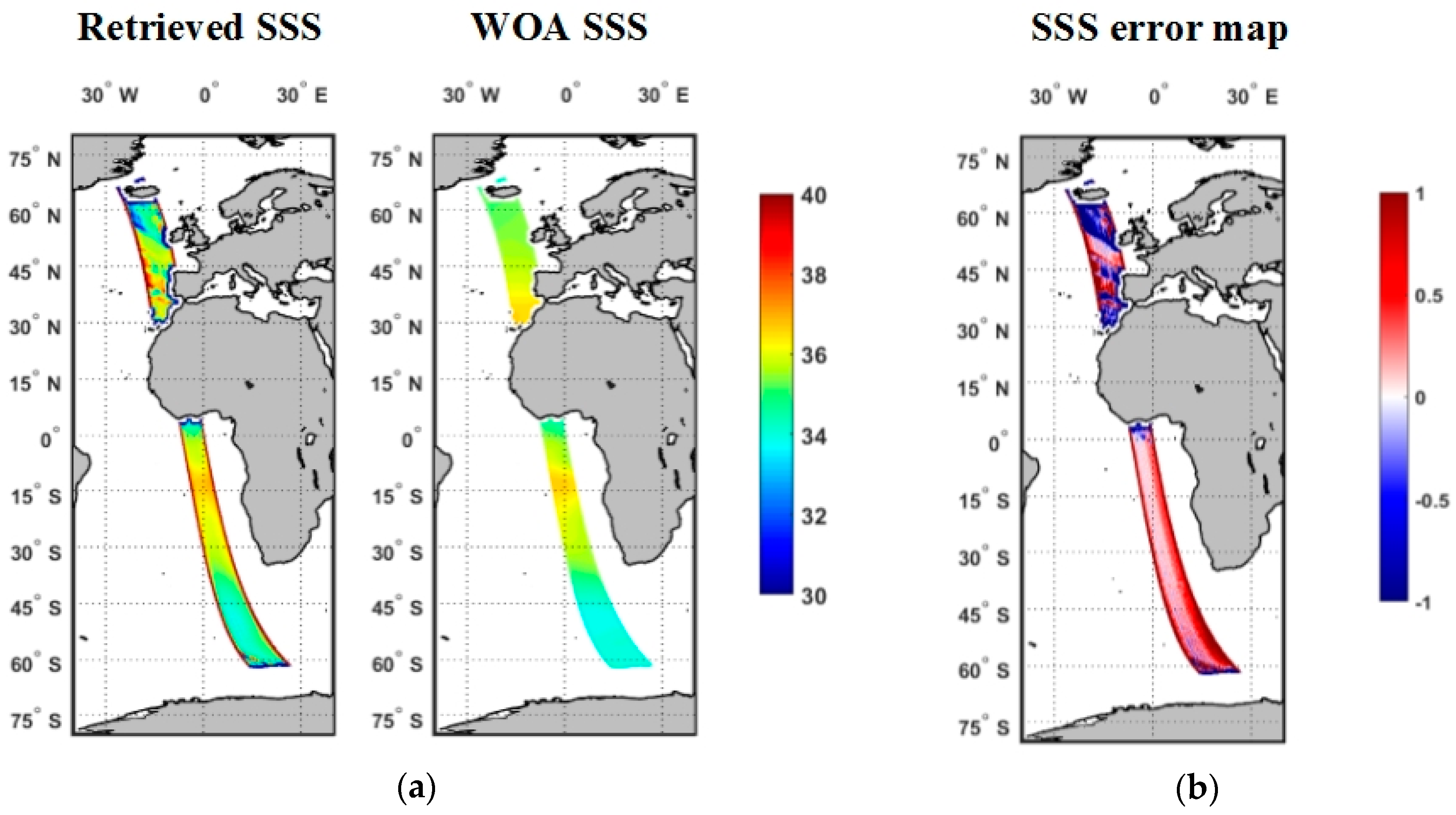
Figure 7a presents the half-orbital (about 2930 measurements) results of the SSS retrieval and the original WOA SSS, while their difference is shown in Figure 7b.
As can be seen from Figure 7, although the SSS retrieval results in the center of the orbit and in the open sea (not near land or poles) are proven to be good, there are large errors, especially at the edge of the orbit and when approaching land. Those errors in the results can be attributed to the aliasing effect, instrument imperfection, and the TB retrieval algorithm. Although TB measured from observation angles of −55°–55° are treated as AF-FOV and are used to retrieve SSS, the results still presented large errors near −55° and 55° due to the low sensitivity of TB to SSS. Even small errors in the reconstructed TB introduced large errors to the retrieved SSS.
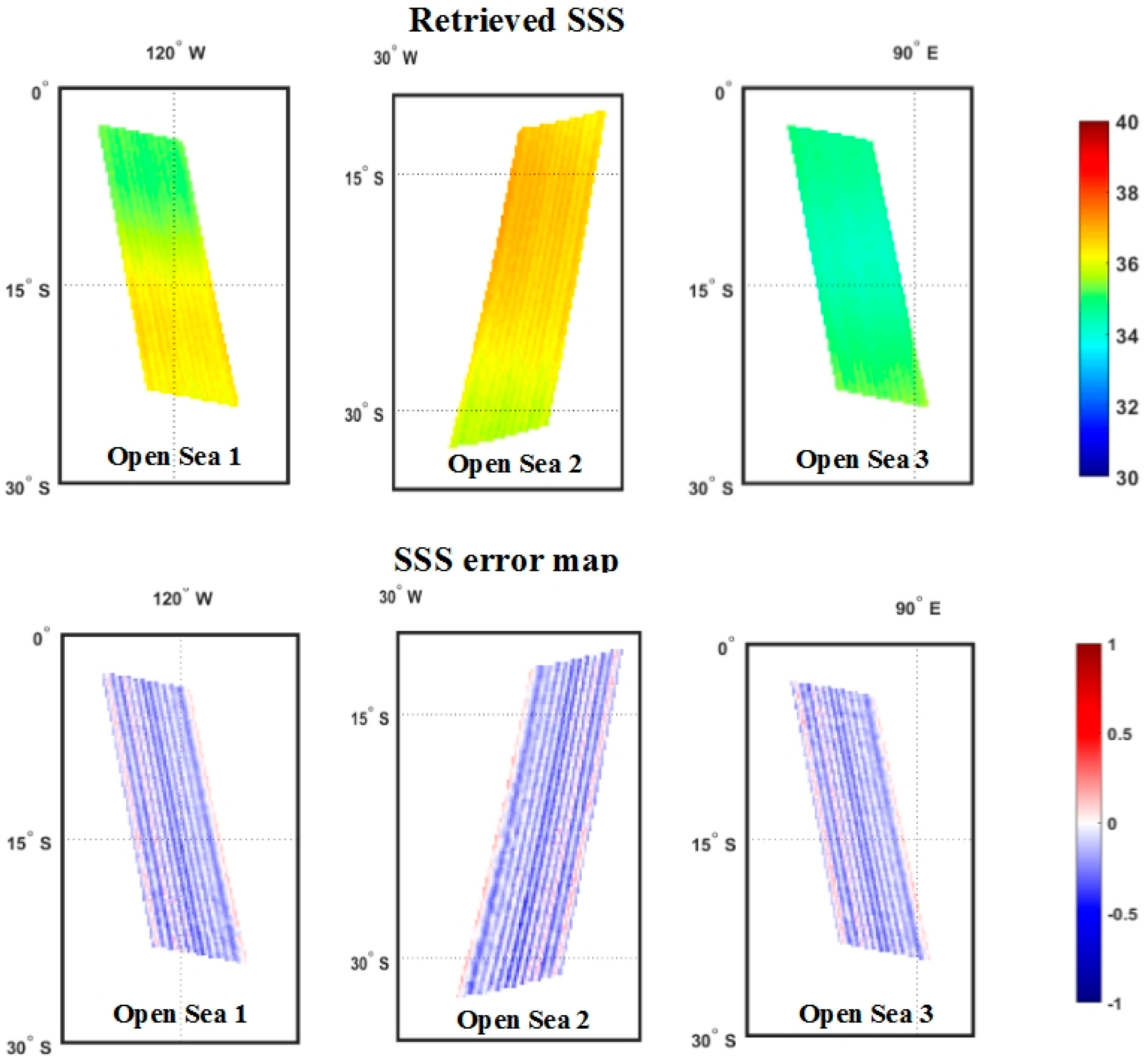
To focus on the retrieval results in open sea, orbital SSS retrieval results from the South Pacific Ocean, South Atlantic Ocean, and Indian Ocean—namely Open Sea 1, 2, and 3, respectively—are selected in this study. Figure 8 presents the retrieved SSS of the three open sea areas on the top row and the corresponding error maps compared with the WOA SSS data on the bottom row. To avoid the large errors around the edge of the orbital results, a narrower AF-FOV the from an observation angle of −45–45° are adopted for the retrieval in the three open sea areas.
As seen from Figure 8, the retrieval results in open sea are much better than the whole half-orbital result in Figure 7. Table 2 displays quantitative results of the retrieved SSS in the three open sea areas, including their RMSE and standard deviations (std). From the quantitative analysis, the accuracy of SSS retrieval in open sea is about 0.17 psu, which satisfied the objective of an accuracy of 0.2 psu for salinity observation.
Compared with 2D instruments, such as SMOS/MIRAS, the imaging results of the 1D radiometer system manifested larger Gibbs errors [19], even for the observation of open seas. Also, the situation became worse when approaching land. This can be attributed to the number of antenna elements of the 1D radiometer system (i.e., eight) used in this paper being much less than that used in the SMOS/MIRAS 2-D system (i.e., 69). The reduction of the antenna elements leads to the reduction of baselines and, eventually, results with a more severe sampling truncation in the spatial frequency domain. This is challenging for systems with small scale antenna elements, like our IMI prototype. An improved system, which may consist of more antenna elements in the feed array, will be developed in the future based on the IMI prototype. Although larger scale antenna arrays will reduce the Gibbs error, land contamination in the observations cannot be eliminated. Many studies devoted to reducing land contamination in SMOS have been carried out [20]. Future work will also focus on the correction of land contamination for our designed system.
4. Conclusions
This paper introduces an end-to-end simulation system to verify the capacity of measuring salinity for a designed system IMI, which is a tri-frequency (L-, S-, and C-bands), one-dimensional aperture synthesis radiometer.
The end-to-end simulation system consisted of three main modules: a tri-frequency TB generator, radiometer, and SSS retrieval. First, TB scenes for the three bands are produced by the TB generator module. Then, the reconstructed TB are outputted from the process of the radiometer module. The experimental measurements of the antenna patterns of a ground-based prototype of IMI are used in the radiometer module simulation.
The simulation was based on the actual antenna patterns and distribution of the IMI prototype and included image reconstruction errors. Additionally, it is mentioned that forward model and retrieval apply the same parameters, as well as that no error was considered on the geophysical data. With this configuration, results indicate a RMSE of 0.26 psu for a single measurement in open sea. Large errors near the edge of the orbit and strong land contamination are found in the half orbital SSS retrieval results. The errors in the results can be attributed to the aliasing effect and the low sensitivity of TB to SSS. Then, three areas are selected in order to focus on the retrieval results in open sea. Simulation results in open sea presented a much better accuracy of 0.17 psu.
Besides the possible underestimation due to the aforementioned simulation configuration, large errors existed in SSS retrieval, which mainly originated from a spatial bias in the radiometer system. An improved system that contains more antenna elements will reduce those errors. To achieve better salinity accuracy, land contamination correction must be done in the future.
Author Contributions
H.L. provided concept and parameters of WOCM/IMI; Y.L. and A.Z. established simulation models; Y.L. performed the simulation and tested the simulation results; Y.L. wrote the manuscripts; and H.L. edited the article.
Funding
This research received no external funding.
Acknowledgments
The authors would like to thank Remote Sensing Systems for providing the geophysical data of AMSR-E, and National Oceanic and Atmospheric Administration for providing the in-situ sea surface salinity data of WOA.
Conflicts of Interest
The authors declare no conflict of interest. The founding sponsors had no role in the design of the study; in the collection, analyses, or interpretation of data; in the writing of the manuscript, and in the decision to publish the results.
References
- Shi, J.; Zhao, T.; Du, J.; Ji, D.; Xiong, C.; Dong, X.; Liu, H.; Wang, Z.; Jiang, L.; Du, Y. Observing Earth’s water cycle from space. In Proceedings of the SPIE International Asia-Pacific Environmental Remote Sensing Symposium, Beijing, China, 13–17 October 2014. [Google Scholar]
- Liu, H.; Niu, L.; Wu, L.; Zhang, C.; Zhang, X.; Yin, X.; Wu, J. IMI (Interferometric Microwave Imager): AL/S/C tri-frequency radiometer for Water Cycle Observation Mission (WCOM). In Proceedings of the 2016 IEEE International Geoscience and Remote Sensing Symposium (IGARSS), Beijing, China, 10–15 July 2016. [Google Scholar]
- Kerr, Y.H.; Waldteufel, P.; Wigneron, J.P.; Martinuzzi, J.A.M.J.; Font, J.; Berger, M. Soil moisture retrieval from space: The Soil Moisture and Ocean Salinity (SMOS) mission. IEEE Trans. Geosci. Remote Sens. 2001, 39, 1729–1735. [Google Scholar] [CrossRef]
- Lagerloef, G.; Colomb, F.R.; Le Vine, D.; Wentz, F.; Yueh, S.; Ruf, C.; Lilly, J.; Gunn, J.; Chao, Y.; Feldman, G.; et al. The Aquarius/SAC-D mission: Designed to meet the salinity remote-sensing challenge. Oceanography 2008, 21, 68–81. [Google Scholar] [CrossRef]
- Entekhabi, D.; Njoku, E.; O’Neill, P.; Spencer, M.; Jackson, T.; Entin, J.; Im, E.; Kellogg, K. The soil moisture active/passive mission (SMAP). In Proceedings of the IGARSS 2008 IEEE International Geoscience and Remote Sensing Symposium, Boston, MA, USA, 7–11 July 2008; Volume 3. [Google Scholar]
- Yueh, S.H.; West, R.; Wilson, W.J.; Li, F.K.; Njoku, E.G.; Rahmat-Samii, Y. Error sources and feasibility for microwave remote sensing of ocean surface salinity. IEEE Trans. Geosci. Remote Sens. 2001, 39, 1049–1060. [Google Scholar] [CrossRef]
- Jin, M.; Liu, H.; Wu, L.; Wu, L.; Wang, R.; Zhang, C.; Yin, X.; Zhao, T.; Sun, W.; Cui, H.; et al. Task Simulation and External Error Sources Analysis for an Ocean Salinity Mission with One-dimensional Synthetic Aperture Microwave Radiometer. Remote Sens. Technol. Appl. 2017, 32, 346–355. [Google Scholar]
- Zine, S.; Boutin, J.; Font, J.; Reul, N.; Waldteufel, P.; Gabarró, C.; Tenerelli, J.; Vergely, J.-L.; Talone, M.; Delwart, S.; et al. Overview of the SMOS Sea Surface Salinity Prototype Processor. IEEE Trans. Geosci. Remote Sens. 2008, 46, 621–645. [Google Scholar] [CrossRef] [Green Version]
- Klein, L.; Swift, C.T. An improved model for the dielectric constant of sea water at microwave frequencies. IEEE Trans. Antennas Propag. 1977, 25, 104–111. [Google Scholar] [CrossRef]
- Meissner, T.; Wentz, F.J. The emissivity of the ocean surface between 6 and 90 GHz over a large range of wind speeds and Earth incidence angles. IEEE Trans. Geosci. Remote Sens. 2012, 50, 3004–3026. [Google Scholar] [CrossRef]
- Wentz, F.J. A two-scale scattering model for foam-free sea microwave brightness temperatures. J. Geophys. Res. 1975, 80, 3441–3446. [Google Scholar] [CrossRef]
- Wentz, F.J.; Meissner, T. AMSR Ocean Algorithm, Algorithm Theoretical Basis Document; Remote Sensing System: Santa, Rosa, CA, USA, 2000. [Google Scholar]
- Corbella, I.; Duffo, N.; Vall-llossera, M.; Camps, A.; Torres, F. The visibility function in interferometric aperture synthesis radiometry. IEEE Trans. Geosci. Remote Sens. 2004, 42, 1677–1682. [Google Scholar] [CrossRef] [Green Version]
- Vall-Llossera Ferran, M.M.; Corbella Sanahuja, I.; Torres Torres, F.; Camps Carmona, A.J.; Colliander, A.; Martín Neira, M.; Ribó Vedrilla, S.; Rautiainen, K.; Duffo Ubeda, N. MIRAS end-to-end calibration: Application to SMOS L1 processor. IEEE Trans. Geosci. Remote Sens. 2005, 43, 1126–1134. [Google Scholar]
- Corbella, I.; Torres, F.; Camps, A.; Duffo, N.; Vall-llossera, M. Brightness-Temperature Retrieval Methods in Synthetic Aperture Radiometers. IEEE Trans. Geosci. Remote Sens. 2009, 47, 285–294. [Google Scholar] [CrossRef] [Green Version]
- Tanner, A.B.; Swift, C.T. Calibration of a synthetic aperture radiometer. IEEE Trans. Geosci. Remote Sens. 1993, 31, 257–267. [Google Scholar] [CrossRef]
- AMSR2/AMSR—Remote Sensing Systems. Available online: http://www.remss.com/missions/amsr/ (accessed on 1 September 2018).
- World Ocean Atlas 2013 Version 2. Available online: https://www.nodc.noaa.gov/OC5/woa13/ (accessed on 1 September 2018).
- Zhang, A.; Liu, H.; Wu, L.; Wu, J.; Niu, L.; Guo, X. Spatial Bias Analysis and Calibration for the L- band 1-D Synthetic Aperture Radiometer. J. Remote Sens. under review.
- Li, Y.; Li, Q.; Lu, H. Land Contamination Analysis of SMOS Brightness Temperature Error Near Coastal Areas. IEEE Geosci. Remote Sens. Lett. 2017, 14, 587–591. [Google Scholar] [CrossRef]
Figure 1.
The end-to-end simulation system of sea surface salinity (SSS) for the tri-frequency one-dimensional interferometric microwave imager, which consists of three major modules highlighted as grey cases at the top (i.e., the brightness temperature (TB) generation module, radiometer module, and sea surface salinity (SSS) retrieval module).

Figure 2.
A ground-based prototype of the one-dimensional interferometric microwave imager (IMI). (a) Photo of the ground-based IMI prototype. (b) Arrangement of the small and large antenna units in the feed array of the IMI prototype.
Figure 2.
A ground-based prototype of the one-dimensional interferometric microwave imager (IMI). (a) Photo of the ground-based IMI prototype. (b) Arrangement of the small and large antenna units in the feed array of the IMI prototype.

Figure 3.
The antenna pattern of the eight-element prototype of the 1D IMI, including the along-track and cross-track antenna patterns in (a) and (b), respectively.
Figure 3.
The antenna pattern of the eight-element prototype of the 1D IMI, including the along-track and cross-track antenna patterns in (a) and (b), respectively.

Figure 4.
TB scenes from the forward TB generation module used as the input of the radiometer simulation. From left to right, the L-, S-, and C-band TB are presented. The horizontal and vertical TB are presented on the top and bottom row, respectively.
Figure 4.
TB scenes from the forward TB generation module used as the input of the radiometer simulation. From left to right, the L-, S-, and C-band TB are presented. The horizontal and vertical TB are presented on the top and bottom row, respectively.

Figure 5.
L-band reconstructed TB output from the radiometer simulation. The blue solid line and the black dashed line present the reconstructed TB and original simulated TB, respectively. From left to right are the horizontal polarization (H-pol), cross polarization (HV-pol, VH-pol), and vertical polarization (V-pol) results.

Figure 6.
Comparison results of retrieval SSS and World Ocean Atlas (WOA) salinity, which are represented by the red stars and the blue circles, respectively.
Figure 6.
Comparison results of retrieval SSS and World Ocean Atlas (WOA) salinity, which are represented by the red stars and the blue circles, respectively.

Figure 7.
(a) Half-orbital SSS retrieval result and the WOA salinity, and (b) corresponding error map when compared with WOA salinity.
Figure 7.
(a) Half-orbital SSS retrieval result and the WOA salinity, and (b) corresponding error map when compared with WOA salinity.

Figure 8.
Simulation results of the orbital retrieved SSS in the three selected open sea areas. SSS retrieval results and the corresponding SSS error maps compared with WOA salinity are shown in the top and bottom rows, respectively.
Figure 8.
Simulation results of the orbital retrieved SSS in the three selected open sea areas. SSS retrieval results and the corresponding SSS error maps compared with WOA salinity are shown in the top and bottom rows, respectively.


Table 1.
Interferometric microwave imager (IMI) design characteristics for Water Cycle Observation Mission (WCOM).
Table 1.
Interferometric microwave imager (IMI) design characteristics for Water Cycle Observation Mission (WCOM).
| L-band | S-band | C-band | |
|---|---|---|---|
| Frequency (GHz) | 1.4135 | 2.695 | 6.9 |
| Bandwidth (MHz) | 25 | 8 | 200 |
| Along-track Resolution (km) | 35 | 20 | 10 |
| Cross-track Resolution (km) | 35–75 | 20–45 | 15–30 |
| Radiometric Resolution (K) | 0.2 | 1.5 | 0.6 |
| Field of View (km) | 1000 | 1000 | 1000 |
Table 2.
Root mean square error (RMSE) and standard deviation (std) of the retrieved SSS for the three selected open sea areas.
Table 2.
Root mean square error (RMSE) and standard deviation (std) of the retrieved SSS for the three selected open sea areas.
| Open Sea | 1 | 2 | 3 |
|---|---|---|---|
| Area Location | South Pacific Ocean | South Atlantic Ocean | Indian Ocean |
| RMSE (psu) | 0.1680 | 0.1779 | 0.1655 |
| std (psu) | 0.1209 | 0.1296 | 0.1209 |
© 2019 by the authors. Licensee MDPI, Basel, Switzerland. This article is an open access article distributed under the terms and conditions of the Creative Commons Attribution (CC BY) license (http://creativecommons.org/licenses/by/4.0/).
Share and Cite
MDPI and ACS Style
Li, Y.; Liu, H.; Zhang, A. End-to-End Simulation of WCOM IMI Sea Surface Salinity Retrieval. Remote Sens. 2019, 11, 217. https://doi.org/10.3390/rs11030217
AMA Style
Li Y, Liu H, Zhang A. End-to-End Simulation of WCOM IMI Sea Surface Salinity Retrieval. Remote Sensing. 2019; 11(3):217. https://doi.org/10.3390/rs11030217
Chicago/Turabian StyleLi, Yan, Hao Liu, and Aili Zhang. 2019. "End-to-End Simulation of WCOM IMI Sea Surface Salinity Retrieval" Remote Sensing 11, no. 3: 217. https://doi.org/10.3390/rs11030217
Note that from the first issue of 2016, this journal uses article numbers instead of page numbers. See further details here.