How Far Can Consumer-Grade UAV RGB Imagery Describe Crop Production? A 3D and Multitemporal Modeling Approach Applied to Zea mays

Abstract

In recent decades, remote sensing has increasingly been used to estimate the spatio-temporal evolution of crop biophysical parameters such as the above-ground biomass (AGB). On a local scale, the advent of unmanned aerial vehicles (UAVs) seems to be a promising trade-off between satellite/airborne and terrestrial remote sensing. This study aims to evaluate the potential of a low-cost UAV RGB solution to predict the final AGB of Zea mays. Besides evaluating the interest of 3D data and multitemporality, our study aims to answer operational questions such as when one should plan a combination of two UAV flights for AGB modeling. In this case, study, final AGB prediction model performance reached 0.55 (R-square) using only UAV information and 0.8 (R-square) when combining UAV information from a single flight with a single-field AGB measurement. The adding of UAV height information to the model improves the quality of the AGB prediction. Performing two flights provides almost systematically an improvement in AGB prediction ability in comparison to most single flights. Our study provides clear insight about how we can counter the low spectral resolution of consumer-grade RGB cameras using height information and multitemporality. Our results highlight the importance of the height information which can be derived from UAV data on one hand, and on the other hand, the lower relative importance of RGB spectral information.

1. Introduction

Maize, rice, and wheat provide 30% of the food calories to more than 4.5 billion people in almost 100 developing countries [1]. Grain yield related to these major crops is therefore one of the most important issues related to national food security and personal living standards [2]. Therefore, accurate crop yield forecasts prior to harvest would enable planners to take more sound and reasonable decisions regarding national food policy [3].

At the local and farm scale, the estimation of crop biomass production is of great importance and remains one of the basic indicators to assess the performance of agricultural practices (e.g., crop response to tillage or residue management [4]), to study environmental processes in the agro-ecosystem (e.g., estimation of carbon stocks or light use efficiency [5]), to analyze plant health status (e.g., estimation of crop losses due to disease severity), to predict and plan logistical aspects (e.g., estimating feed production available on the farm, or planning grain delivery and stock in grain depots) or for the purpose of precision agriculture (e.g., site-specific N management [6]).

In such a global and local context, techniques allowing for a rapid, economical and quantitative estimation of crop biomass and yield production are therefore of great importance for accessibility risk management, global markets, policy-making, and decision-making from farm over regional to even global scale [7].

Remote sensing is increasingly used to estimate the spatio-temporal evolution of crop biophysical parameters, thanks to its ability to collect non-destructive time-lapse information over large area [8]. Satisfactory relationships have been proposed in the literature between remotely sensed spectral variables, usually combined in and expressed through vegetation indices (VI), and crop biophysical parameters such as phenology [9], leaf area index (LAI [10]), and above-ground biomass (AGB [11]).

The Near InfraRed (NIR) spectral band is by far the most used in VI’s, because of the reflection characteristic of this spectral band by green vegetation, in comparison to the reflection in the visible bands: Red (R), Green (G) or Blue (B). Even though they are smaller, spectral differences in the reflectance in the visible bands exist, and are caused by biochemical plant constituents such as chlorophyll [12,13], allowing for RBG-derived VI’s to be properly used for agronomical purposes as well. However, in both the NIR-based and RGB-based indices, the spectral signals of remotely sensed images tend to saturate with vegetation biomass where or when canopy densities become too important. Furthermore, reference [14] reported that small changes in leaf orientation could induce important modifications in the spectral composition and intensity.

Biomass estimation is commonly recognized as being crucial for yield prediction of crops [15], and for certain agricultural species such as maize, accurate determination of the crop height has also been proven to be a very good indicator of the actual plant biomass [8] or the upcoming crop yields [16]. Plant height information is most useful when it is available at high spatial and temporal resolution, but in situ physical measurements are laborious and it can be difficult to properly characterize the spatial variability [17]. As an alternative to physical measurement methods of crop heights, several studies have investigated remote sensing as an alternative for crop height measurement. In terms of remote sensing approach, LiDAR [8,18] and structure from motion photogrammetry [13] are the most common. These methods can be implemented on aerial platforms (unmanned and manned aircraft) or by a human operator on the ground.

The recent advent of unmanned aerial vehicles (UAVs) seems to be a promising trade-off between satellite/airborne and terrestrial remote sensing in the study of agronomical and ecological management. Both non-imaging (e.g., LiDAR) and imaging (e.g., RGB camera, multispectral or hyperspectral) sensors can be mounted on UAV. A detailed presentation on the evolution and state-of-the-art discussion of the use of UAV systems is presented in Colomina and Molina [19].

Recently, photogrammetric imaging using UAV’s, supported by the structure of motion (SfM) technique and dense image matching has become very interesting tool to collect 3D information of objects due to its low cost, efficiency, flexibility and ability to work in near-real-time [17,20,21]. These methods, in combination or not with spectral data, have already been investigated in different studies regarding e.g., winter barley [11,13,22], winter wheat [23] or maize [8] crop production. Nevertheless, those studies did not investigate the use of combinations of RGB vegetation indices and UAV Crop Height data to predict AGB considering various growing stages. They also did not provide insight about the added value of UAV imagery in terms of AGB modeling when compared with classical field measured parameters (e.g., intermediate AGB).

The main goal of our study is to evaluate the potential of multitemporal UAV imagery to predict AGB of maize using a consumer-grade UAV and RGB camera. More specifically, our study aims to: (i) evaluate the added value of 3D data derived from photogrammetric reconstruction using the same source imagery data, (ii) give insight about the best (combination of) time windows to perform UAV flight survey to predict AGB, (iii) compare the added value of UAV imagery with field measure of AGB in order to predict the AGB of the crop. We tested this approach on a corn field in Belgium.

2. Materials and Methods

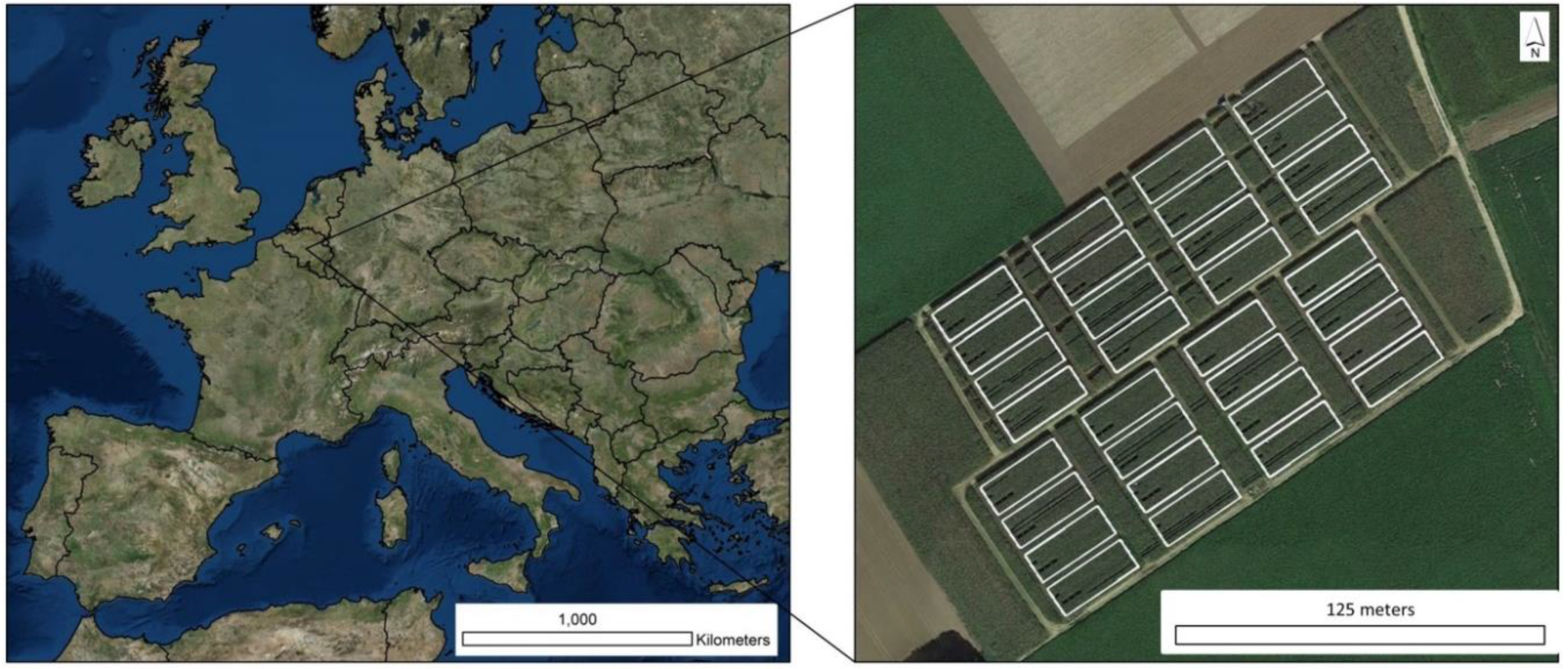
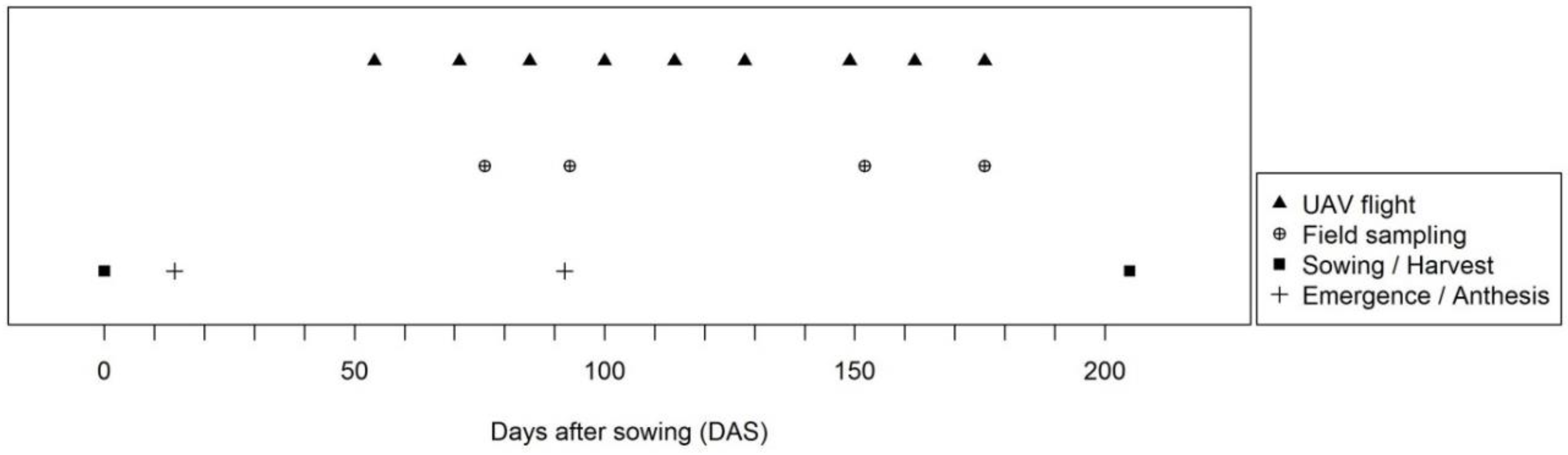
2.1. Study Site and Field Measurements

The study site consisted of 32 experimental plots (15 × 40 m) of maize (Zea mays L.) installed in Gembloux (Wallonia, Southern Belgium—50°33′50.75″N, 4°42′46.4″E, Figure 1). The crop was sown on 21 and 22 April 2015 and harvested on 13 November 2015 (see Figure 2). The emergence and the anthesis occurred on 6 May and 23 July, respectively.

The total AGB was measured on each plot four times during the growing season (see Figure 2). We took destructive crop samples (quadrat method) which were weighted after drying. For each sample, an associated area was computed based on the outdistance sowing and the number of sampled crops to approximate an AGB measurement per area unit. Details of data sampling can be found in [4].

2.2. Acquisition and Pre-Processing of UAV Imagery

We used an octocopter drone (X frame type) carrying an off-the-shelf high spatial resolution (20 Mpx) RGB camera (Sony RX 100 mk3). The octocopter’s flight height was set to 50 m above ground level, with a cruise speed at 5 m·s⁻¹ and a front and a side overlaps above 80%. Nine flight surveys were performed every two weeks, from the 15 June to the 15 October 2015 (see Figure 2). This schedule was established as a balance between surveying the crops at various growth stages and the operational complexity of regular flight surveys (e.g., meteorological conditions or manpower). The swath of the UAV individual images was ca. 75 m and the total area covered by a single flight survey was ca. 42,000 m².

We set 16 Ground Control Points (GCP) consisting of 0.4 m white square plastic plates in the surveyed area to ensure geometric calibration. The GCP were georeferenced with a GPS Leica ATX1230 (±0.01 m mean XYZ accuracy).

We used Agisoft PhotoScan Professional (version 1.2, see http://www.agisoft.com/) to perform a photogrammetric 3D reconstruction of the acquired imagery for every flight survey. Two UAV raster products derived from each flight were RGB orthophotomosaic and Digital Surface Model (DSM). The Ground Sampling Distance (GSD) was 0.02 m for RGB orthophotomosaic and 0.05 m for the DSM.

The geometric accuracy of the UAV products is optimized using the reference data provided by the 16 GCP. Agisoft Photoscan performs a self-calibration process to refine the camera parameters to match theses reference data. Following the approach proposed by James et al. [24], we selected the following set of parameters in the optimization process: focal distance (f), principal point (cx cy), tangential distortion (k1 to k3), radial distortion (p1 p2) and affinity/skew coefficients (b1 b2). Such approaches are widely used in environmental sciences (e.g., [25,26]) to derive UAV mapping products presenting high georeferencing and geometric quality.

We produced a Crop Height Model (CHM) by subtracting a LiDAR DTM to the high spatial resolution photogrammetric DSM to provide a raster of the crop height (0.02 m GSD). The public regional administration (see http://geoportail.wallonie.be/ for further information) extracted a LiDAR DTM from LiDAR survey (<1 point/m²) acquired during the years 2013 and 2014. As the trial occurred in 2015, the LiDAR DTM from the regional survey was considered as still relevant to describe the topography of the study area.

2.3. Modeling Final AGB with UAV Imagery

Partial least-square (PLS) regressions were used to investigate the relationship between multitemporal UAV imagery and the AGB through three different modeling approach directly linked to the three specific sub-objectives of the study. The “plsdepot” package [27] implemented in the R software [28] was used for the modeling tasks. The PLS regression modeling is used to find the relations between two matrices (X and Y) and present the advantage to be more robust than linear regression and principal component regression methods [29]. PLS regression modeling is also less affected by data collinearity and represents a valuable method for modeling high-dimensional data [30].

2.3.1. Data Preparation

The field measured AGB observations were linearly interpolated to the flight times (time-based interpolation) to match the timing of field AGB acquisition with the nine dates associated with UAV flight surveys. The AGB interpolated for the 15 October (last UAV flight) will be further referred to the final AGB measurement.

For every UAV flight survey, a median value was extracted for the Red, Green and Blue channels of the corresponding orthophotomosaic within the 32 field plots. The median values are divided by the associated brightness (Median Red + Median Green + Median Blue) to reduce the impact of changing sunlight condition during the flight surveys.

Median plant height values were also extracted for the 32 field plots, based on the CHM raster. To enhance contrast and reduce the spectral heterogeneity, we computed five spectral indices, which are listed in

Table 1. Vegetation indices computed from median luminescence value normalized by brightness.

Reference	Formula	Source
NGRDI—Normalized Green Red Difference Index	(GREEN − RED)/(GREEN + RED)	[31]
NGBI—Normalized Green Blue Index	(GREEN − BLUE)/(GREEN + BLUE)	[32]
NRBI—Normalized Red Blue Index	(RED − BLUE)/(RED + BLUE)	[32]
VARI—Visible Atmospherically Resistant Index	(GREEN − RED)/(GREEN + RED − BLUE)	[33,34]
TGI—Triangular Greenness Index	GREEN − (0.39 × RED) − (0.61 × BLUE)	[35,36]

. The spectral indices cover the spectral ranges of the camera used for this study and were chosen because of their simplicity and replicability. They were used as predictors within the constructed model instead of the original luminescence value from the RGB orthophotomosaic and were computed for each plot for the 9 UAV flight survey dates.

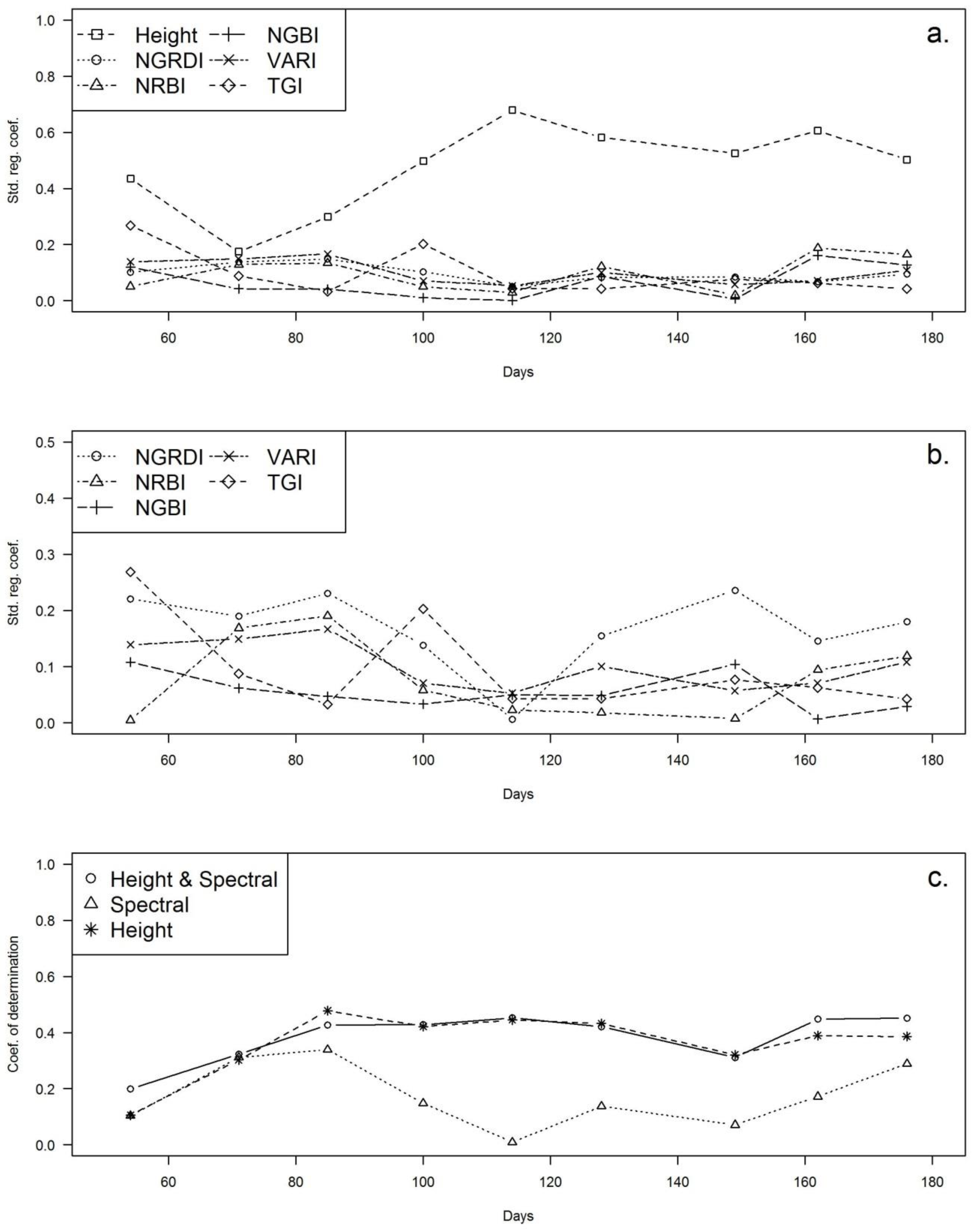
2.3.2. Modeling Approach 1: 3D Data vs. Spectral UAV Data

The orthophotomosaic and the DSM are the two basics products that can be produced with overlapping images acquired by a UAV. In this paper, we combined the obtained DSM information with a LiDAR DTM to produce CHM. Multitemporal CHMs provide insight about the vertical development and the growth rate of the crops. To evaluate the added value of 3D data, the final AGB was firstly modeled using a mixed approach (3D and spectral UAV data, Model 1a) and secondly based on spectral UAV data only (Model 1b). A PLS regression model was adjusted for every flight survey where the index _i represents the considered UAV flight date.

$$Model 1a: \mathrm{Final}\mathrm{AGB}=f\left({\mathrm{Median}\mathrm{Height}}_i+{\mathrm{NGRDI}}_i+{\mathrm{NGBI}}_i+{\mathrm{NRBI}}_i+{\mathrm{TGI}}_i+{\mathrm{VARI}}_i\right);$$

$$Model 1b:\mathrm{Final}\mathrm{AGB}=f\left({\mathrm{NGRDI}}_i+{\mathrm{NGBI}}_i+{\mathrm{NRBI}}_i+{\mathrm{TGI}}_i+{\mathrm{VARI}}_i\right);$$

$$Model 1c:\mathrm{Final}\mathrm{AGB}=f\left({\mathrm{Median}\mathrm{Height}}_i\right);$$

where the index i represents the UAV flight date.

For each model, we used the standardized regression coefficients of the UAV variables to highlight their individual contribution to the model and their temporal evolution. Higher the standardized regression coefficients of one variable is, higher the contribution of this variable to the model is. The same approach was used with the R-square (sum of the two first components) to understand the quality of the final AGB models associated with each UAV flight survey date.

2.3.3. Modeling Approach 2: Timing of UAV Acquisition

Based on the most suitable option in terms of UAV products previously identified, this section investigates how two UAV flight surveys can be combined to predict the final AGB. As the combination of nine flights is most probably too time-consuming for operational application, we used a flights combination of two flights which is closer to a potential field application. For this purpose, a final AGB model was developed for every combination of two flying dates, using the corresponding UAV variables. For each model, the R-square (sum of the two first components) was used to understand the quality of the final AGB prediction associated with each combination of two flights. In the formulas here below, UAV variables₁ regroups the UAV products corresponding with date 1. Depending on the results associated with the modeling approach 1, the UAV products can be 3D and/or spectral.

Modeling approach 2:

$$\mathrm{Final}\mathrm{AGB}=f\left({\mathrm{UAV}\mathrm{variables}}_1+{\mathrm{UAV}\mathrm{variables}}_2\right)$$

$$\mathrm{Final}\mathrm{AGB}=f\left({\mathrm{UAV}\mathrm{variables}}_1+{\mathrm{UAV}\mathrm{variables}}_3\right)$$

$$\mathrm{Final}\mathrm{AGB}=f\left({\mathrm{UAV}\mathrm{variables}}_1+{\mathrm{UAV}\mathrm{variables}}_4\right)$$

…

$$\mathrm{Final}\mathrm{AGB}=f\left({\mathrm{UAV}\mathrm{variables}}_7+{\mathrm{UAV}\mathrm{variables}}_8\right)$$

2.3.4. Modeling Approach 3: UAV Data vs. Field Data

The last modeling approach investigates the added value of AGB field measurements in addition to the UAV imagery variables to predict the final AGB of the crop. The quality of the final AGB prediction was evaluated based on predictors combining intermediate field AGB (single date) data with a later UAV variable (single date). It was decided to use the interpolated AGB observations which presented a higher frequency, to see what the most relevant date would be to perform a sampling, if the approach was found to be successful.

To complete this analysis, we compared this to a strictly ground-based approach (i.e., prediction of final AGB with single intermediate field AGB) and to a strictly UAV-based approach (i.e., prediction of final AGB with UAV variables associated with a single UAV flight survey).

Modeling approach 3:

$$\mathrm{Final}\mathrm{AGB}=f\left({\mathrm{AGB}\mathrm{sampling}}_1+{\mathrm{UAV}\mathrm{variables}}_2\right)$$

$$\mathrm{Final}\mathrm{AGB}=f\left({\mathrm{AGB}\mathrm{sampling}}_1+{\mathrm{UAV}\mathrm{variables}}_3\right)$$

$$\mathrm{Final}\mathrm{AGB}=f\left({\mathrm{AGB}\mathrm{sampling}}_1+{\mathrm{UAV}\mathrm{variables}}_4\right)$$

…

$$\mathrm{Final}\mathrm{AGB}=f\left({\mathrm{AGB}\mathrm{sampling}}_7+{\mathrm{UAV}\mathrm{variables}}_8\right)$$

3. Results

3.1. Modeling Approach 1: 3D Data vs. Spectral UAV Data

The Figure 3 shows the result of modeling approach 1 (mixed final AGB model). In Figure 3a we can see that the mixed models based on different spectral indices and crop height vary slightly among each other but behave similarly over time. Nevertheless, adding height information to the model improves the quality of the AGB prediction, especially after 100 days after sowing (DAS). The lower relative interest for height data in the early growing stages (before 100 DAS) can be linked to the lower height differences between individual crops at the beginning of the crop growth. The interest of spectral data can mainly be associated with the early crop development stages. Figure 3b highlights the performance of models only based on spectral information. There is no particular individual index performing clearly better than the others and their performance depends on the growing stage of the crop. UAV data acquired more than 80 DAS does not contribute notably to the quality of the final AGB prediction (Figure 3c). Since the combination of both data (spectral and height) works out best, this set-up was kept for the following modeling activities.

3.2. Modeling Approach 2: Timing of UAV Acquisition

Table 2. Modeling the final AGB with the combination of UAV variables (vegetation indices and height) from two flight surveys. Each cell represents the R-square (sum of the two pls components) associated with the final AGB model adjusted with the combination of UAV variables from two flight dates. For every flight date, the best combination is bolded and marked with a * character.

Flight Date (Days after Seeding)		UAV Variables
		54	71	85	100	114	128	149	162	176
UAV variables	54	0.2	0.35	0.46	0.55 *	0.52	0.44	0.42	0.52	0.47
	71		0.32	0.41	0.43	0.39	0.44 *	0.38	0.43	0.43
	85			0.43	0.49 *	0.46	0.47	0.46	0.48	0.47
	100				0.43	0.47 *	0.46	0.42	0.46	0.46
	114					0.45	0.43	0.40	0.47 *	0.47
	128						0.42	0.37	0.46	0.49 *
	149							0.31	0.39	0.45 *
	162								0.45	0.47 *
	176									0.45 *

investigates how data computed from two selected UAV flight surveys can be combined to predict the final AGB. When two flight dates are the same (values in the diagonal), the R-square value corresponds to the value associated with the single date model (Figure 3c).

The best performing combinations (e.g., 54 and 100 DAS) reached 0.55 (R-square). While the absolute gain might seem little in some cases (e.g., when compared to a single flight at 100 or 114 DAS, which yielded respectively R-squared of 0.43 and 0.45), performing two flights provides an improvement in AGB prediction ability in comparison to most single flights (>90% of potential combinations). As an example, performing a flight at 71 and 128 DAS (R-square of 0.44) is better than flying only at 149 DAS (R-square of 0.31).

3.3. Modeling Approach 3: UAV Data vs. Field Data

Table 3. Modeling the final AGB with the combination of UAV variables (vegetation indices and height) provided by a single flight survey with an intermediate field AGB measurement. Each cell represents the R-square (sum of the two pls components) associated with the final AGB model adjusted with the considered combination. The last row (bolded values) represents the R-square (sum of the two pls components) of final AGB models build with single date UAV products. The last column represents the R-square (sum of the two pls components) of final AGB models build with single date intermediate field AGB values. For every flight date, the best combination is marked with the * character.

Flight Date (DAS)		UAV Variables
		54	71	85	100	114	128	149	162	176	Pred. Final AGB with Field AGB
Field AGB	54		0.35	0.43	0.42	0.41	0.41	0.34	0.42	0.46 *	0.29
	71			0.43	0.42	0.41	0.41	0.34	0.42	0.46 *	0.29
	85				0.46	0.45	0.44	0.38	0.46	0.48 *	0.38
	100					0.48	0.47	0.41	0.48	0.50 *	0.43
	114						0.52	0.45	0.53 *	0.52	0.48
	128							0.48	0.56 *	0.53	0.49
	149								0.58 *	0.52	0.44
	162									0.8 *	0.82
	176										1
Pred. Final AGB with UAV		0.20	0.32	0.43	0.43	0.45	0.42	0.31	0.45	0.45

shows the added value of UAV imagery (spectral and height data) to predict the final AGB if a previous field measured AGB is available. The reading of the last columns from Table 3 indicates quite logically that the later the field ABG measurement is performed, the more the final AGB prediction is improved. When comparing these values (last column) with the last row of the table, one can also notice that prediction based on field AGB measure or UAV flight are of similar order of accuracy when performed around 100 DAS (0.43). Later in the season, the performance becomes greater with field AGB measures while UAV information remain steady.

Each other row of Table 3 indicates how a given final AGB predication based on intermediate field measured AGB is improved by addition of information gained with a UAV flight performed in between the sampling date and the time of harvest. In most cases the addition of UAV imagery improves the final AGB prediction to a varying extent, but certainly confirming the interest of the approach. Indeed, an early biomass sampling would be much easier to be performed by a farmer and a UAV flight performed latter in the season would offer the spatial variability of the field.

4. Discussions

Crop height derived from 3D imagery appeared as the most interesting predictor of final AGB, in comparison to remotely sensed vegetation indices based on RGB imagery. The importance of crop height as predictor of final yield had been highlighted by [8] which found the crop height to be systematically selected in an automated stepwise variable selection procedures. When the sole mean crop height was used, the model performance (adjusted R-squared) ranged approximately 0.51 with a flight performed ~1.5 month before maize harvest. In our case, when using the sole crop height, we reached comparable model performance, with a steady R-squared observed from 100 days before harvest (i.e., ~100 DAS).

Collecting spectral information at different phenological stages, reference [37] found out that the correlation of different VI with final rice grain yield were almost systematically optimal around booting stage. This confirmed the observation reported, were the maximum correlation with the spectral information was maximal between the DAS 85 and 100 time period which can be associated with the flowering stage in our case (anthesis occurred 92 DAS).

Regarding the combination of plant height estimates and vegetation indices, references [13] found out that the performance of prediction were not improved when crop height information was combined with common VI to predict biomass over multiple dates. Oppositely, in the case study of [8], vegetation indices were found to have an added value in the final set of explanatory variables, in combination with crop height, and improved prediction of AGB. Our observation seemed to highlight an added value of spectral information used in early prediction of final AGB (before half-season, ca. 100 DAS). After that, crop height can be used alone for prediction of final AGB.

Earlier studies have indicated that accumulative VI could improve the stability of yield prediction [2,38]. However, contrarily to the simple VI values accumulation [2], reference [37] had proposed to use a multiple linear regression approach to automatically select the best combination of (two) flying times to predict final rice yield. They found out that combining a flight at jointing or heading stage with a flight at booting stage gave a better correlation with grain yield than did VI obtained at any single growing stage.

Using a systematic analysis of all flight combination, our study confirms these findings and the importance of flying at specific growing stage (flowering stage, in this case). The end of flowering-early grain filling represents the end of the vegetative phase, where the plant enters the reproductive phase. At that moment, maize reaches its vegetative nutrient growth peak [39] and most of the reserve has been acquired, allowing to partially compensate for further potential problem during grain filling phase. Around that time, the LAI is also the highest, and to some point it reflects the maximal photosynthetic capacity of the plant. This explains why many studies reports successful estimates of crop yield using VI indices computed when LAI has reached its maximum [7,37,40].

Yet, it seems that UAV-derived information cannot really outperform the use of in situ field measurements. However, from our results, it seems clear that the combination of information acquired from biomass sampling performed during early growth—when it is quite easy to access the field and when the biomass development might be relatively more homogeneous—and combined with UAV-derived information gathered through a later flight—when it is more complicated to access the field and when the variability is greater between different field zone—present an interesting potential to assess final AGB or yield.

Globally, our results point out the importance of UAV information acquired at the mid-season (100 DAS), around the end of the vegetative phase. Even if this timeslot did not provide the best result in terms of prediction accuracy, it represents the most interesting timeslot in terms of operational application, providing satisfactory final AGB prediction more than 100 days before the actual harvesting.

5. Conclusions

In terms of timing of UAV surveys, our results suggest that the half-season (100 DAS) is the best time windows to predict the final AGB. In this case, study, final AGB prediction model performance reached 0.55 (R-square) using only UAV information and 0.8 (R-square) when combining UAV information from a single flight with a single-field AGB measurement. When assessing the final AGB using consumer-grade UAV-derived information, it seemed, from the different approaches set up, that there is a crucial interest of performing flight mid-season, between flowering and early grain filling, (~100 DAS in this case).

Nevertheless, the crop height reconstruction requires higher computing time and a more specific expertise than the production of spectral information, our results claim that a sound AGB estimation using consumer-grade cameras must rely on height information. In terms of potential operational application, the use of cloud-based solutions and standardized procedure integrating automatic referencing can simplify the production of photogrammetric crop height information. Photogrammetry based on off-the-shelf RGB cameras is still the only low-cost approach to produce 3D information but the development of low-cost LiDAR will open new opportunities, notably relying on completely “onboard” processing workflows.

Our study provides clear insight about how we can counter the low spectral resolution of consumer-grade RGB cameras using height information and multitemporality. Our results highlight the importance of the height information which can be derived from UAV data on one hand, and on the other hand, the lower relative importance of RGB spectral information.

References

1. Shiferaw, B.; Prasanna, B.M.; Hellin, J.; Bänziger, M. Crops that feed the world 6. Past successes and future challenges to the role played by maize in global food security. Food Secur. 2011, 3, 307. [Google Scholar] [CrossRef]
2. Wang, L.; Tian, Y.; Yao, X.; Zhu, Y.; Cao, W. Predicting grain yield and protein content in wheat by fusing multi-sensor and multi-temporal remote-sensing images. Field Crop. Res. 2014, 164, 178–188. [Google Scholar] [CrossRef]
3. Noureldin, N.; Aboelghar, M.; Saudy, H.; Ali, A. Rice yield forecasting models using satellite imagery in Egypt. Egypt. J. Remote Sens. Space Sci. 2013, 16, 125–131. [Google Scholar] [CrossRef]
4. Hiel, M.-P.; Barbieux, S.; Pierreux, J.; Olivier, C.; Lobet, G.; Roisin, C.; Garré, S.; Colinet, G.; Bodson, B.; Dumont, B. Impact of crop residue management on crop production and soil chemistry after seven years of crop rotation in temperate climate, loamy soils. PeerJ 2018, 6, e4836. [Google Scholar] [CrossRef] [PubMed]
5. Li, W.; Niu, Z.; Huang, N.; Wang, C.; Gao, S.; Wu, C. Airborne LiDAR technique for estimating biomass components of maize: A case study in Zhangye City, Northwest China. Ecol. Indic. 2015, 57, 486–496. [Google Scholar] [CrossRef]
6. Basso, B.; Dumont, B.; Cammarano, D.; Pezzuolo, A.; Marinello, F.; Sartori, L. Environmental and economic benefits of variable rate nitrogen fertilization in a nitrate vulnerable zone. Sci. Total Environ. 2016, 545, 227–235. [Google Scholar] [CrossRef] [PubMed] [Green Version]
7. Becker-Reshef, I.; Vermote, E.; Lindeman, M.; Justice, C. A generalized regression-based model for forecasting winter wheat yields in Kansas and Ukraine using MODIS data. Remote Sens. Environ. 2010, 114, 1312–1323. [Google Scholar] [CrossRef]
8. Li, W.; Niu, Z.; Chen, H.; Li, D.; Wu, M.; Zhao, W. Remote estimation of canopy height and aboveground biomass of maize using high-resolution stereo images from a low-cost unmanned aerial vehicle system. Ecol. Indic. 2016, 67, 637–648. [Google Scholar] [CrossRef]
9. Motohka, T.; Nasahara, K.N.; Oguma, H.; Tsuchida, S. Applicability of Green-Red Vegetation Index for Remote Sensing of Vegetation Phenology. Remote Sens. 2010, 2, 2369–2387. [Google Scholar] [CrossRef] [Green Version]
10. Kross, A.; McNairn, H.; Lapen, D.; Sunohara, M.; Champagne, C. Assessment of RapidEye vegetation indices for estimation of leaf area index and biomass in corn and soybean crops. Int. J. Appl. Earth Obs. Geoinf. 2015, 34, 235–248. [Google Scholar] [CrossRef]
11. Bendig, J.; Bolten, A.; Bennertz, S.; Broscheit, J.; Eichfuss, S.; Bareth, G. Estimating biomass of barley using crop surface models (CSMs) derived from UAV-based RGB imaging. Remote Sens. 2014, 6, 10395–10412. [Google Scholar] [CrossRef]
12. Basso, B.; Cammarano, D.; Carfagna, E. Review of crop yield forecasting methods and early warning systems. In Proceedings of the First Meeting of the Scientific Advisory Committee of the Global Strategy to Improve Agricultural and Rural Statistics, Rome, Italy, 18–19 July 2013; pp. 18–19. [Google Scholar]
13. Bendig, J.; Yu, K.; Aasen, H.; Bolten, A.; Bennertz, S.; Broscheit, J.; Gnyp, M.L.; Bareth, G. Combining UAV-based plant height from crop surface models, visible, and near infrared vegetation indices for biomass monitoring in barley. Int. J. Appl. Earth Obs. Geoinf. 2015, 39, 79–87. [Google Scholar] [CrossRef]
14. De Wulf, R. Optical Remote Sensing Methods for Agricultural Crop Growth Monitoring and Yield Prediction. Ph.D. Thesis, RUG, Faculteit Landbouwwetenschappen, Gent, Belgium, January 1992. [Google Scholar]
15. Oerke, E.-C.; Gerhards, R.; Menz, G.; Sikora, R.A. Precision Crop Protection—The Challenge and Use of Heterogeneity; Springer: Berlin/Heidelberg, Germany, 2010; Volume 5. [Google Scholar]
16. Yin, X.; McClure, M.A.; Jaja, N.; Tyler, D.D.; Hayes, R.M. In-season prediction of corn yield using plant height under major production systems. Agron. J. 2011, 103, 923–929. [Google Scholar] [CrossRef]
17. Viljanen, N.; Honkavaara, E.; Näsi, R.; Hakala, T.; Niemeläinen, O.; Kaivosoja, J. A Novel Machine Learning Method for Estimating Biomass of Grass Swards Using a Photogrammetric Canopy Height Model, Images and Vegetation Indices Captured by a Drone. Agriculture 2018, 8, 70. [Google Scholar] [CrossRef]
18. Tilly, N.; Hoffmeister, D.; Cao, Q.; Huang, S.; Lenz-Wiedemann, V.; Miao, Y.; Bareth, G. Multitemporal crop surface models: Accurate plant height measurement and biomass estimation with terrestrial laser scanning in paddy rice. J. Appl. Remote Sens. 2014, 8, 083671. [Google Scholar] [CrossRef]
19. Colomina, I.; Molina, P. Unmanned aerial systems for photogrammetry and remote sensing: A review. ISPRS J. Photogramm. Remote Sens. 2014, 92, 79–97. [Google Scholar] [CrossRef]
20. Leberl, F.; Irschara, A.; Pock, T.; Meixner, P.; Gruber, M.; Scholz, S.; Wiechert, A. Point clouds. Photogramm. Eng. Remote Sens. 2010, 76, 1123–1134. [Google Scholar] [CrossRef]
21. Lisein, J.; Pierrot-Deseilligny, M.; Bonnet, S.; Lejeune, P. A Photogrammetric Workflow for the Creation of a Forest Canopy Height Model from Small Unmanned Aerial System Imagery. Forests 2013, 4, 922–944. [Google Scholar] [CrossRef] [Green Version]
22. Bendig, J.; Bolten, A.; Bareth, G. UAV-based imaging for multi-temporal, very high resolution crop surface models to monitor crop growth variability. Photogramm. Fernerkund. Geoinf. 2013, 2013, 551–562. [Google Scholar] [CrossRef]
23. Yue, J.; Yang, G.; Li, C.; Li, Z.; Wang, Y.; Feng, H.; Xu, B. Estimation of winter wheat above-ground biomass using unmanned aerial vehicle-based snapshot hyperspectral sensor and crop height improved models. Remote Sens. 2017, 9, 708. [Google Scholar] [CrossRef]
24. James, M.R.; Robson, S.; d’Oleire-Oltmanns, S.; Niethammer, U. Optimising UAV topographic surveys processed with structure-from-motion: Ground control quality, quantity and bundle adjustment. Geomorphology 2017, 280, 51–66. [Google Scholar] [CrossRef]
25. Kim, D.-W.; Yun, H.S.; Jeong, S.-J.; Kwon, Y.-S.; Kim, S.-G.; Lee, W.S.; Kim, H.-J. Modeling and Testing of Growth Status for Chinese Cabbage and White Radish with UAV-Based RGB Imagery. Remote Sens. 2018, 10, 563. [Google Scholar] [CrossRef]
26. Harwin, S.; Lucieer, A. Assessing the Accuracy of Georeferenced Point Clouds Produced via Multi-View Stereopsis from Unmanned Aerial Vehicle (UAV) Imagery. Remote Sens. 2012, 4, 1573–1599. [Google Scholar] [CrossRef] [Green Version]
27. Sanchez, G. Package “plsdepot”. Available online: https://cran.r-project.org/web/packages/plsdepot/plsdepot.pdf (accessed on 23 August 2018).
28. R Core Team. R: A Language and Environment for Statistical Computing; R Foundation for Statistical Computing: Vienna, Austria, 2017. [Google Scholar]
29. Geladi, P.; Kowalski, B.R. Partial least-squares regression: A tutorial. Anal. Chim. Acta 1986, 185, 1–17. [Google Scholar] [CrossRef]
30. Palermo, G.; Piraino, P.; Zucht, H.-D. Performance of PLS regression coefficients in selecting variables for each response of a multivariate PLS for omics-type data. Adv. Appl. Bioinform. Chem. 2009, 2, 57. [Google Scholar] [CrossRef] [PubMed]
31. Hunt, E.R.; Doraiswamy, P.C.; McMurtrey, J.E.; Daughtry, C.S.; Perry, E.M.; Akhmedov, B. A visible band index for remote sensing leaf chlorophyll content at the canopy scale. Int. J. Appl. Earth Obs. Geoinf. 2013, 21, 103–112. [Google Scholar] [CrossRef] [Green Version]
32. Michez, A.; Piégay, H.; Lisein, J.; Claessens, H.; Lejeune, P. Classification of riparian forest species and health condition using multi-temporal and hyperspatial imagery from unmanned aerial system. Environ. Monit. Assess. 2016, 188. [Google Scholar] [CrossRef] [PubMed] [Green Version]
33. Gitelson, A.A.; Viña, A.; Arkebauer, T.J.; Rundquist, D.C.; Keydan, G.; Leavitt, B. Remote estimation of leaf area index and green leaf biomass in maize canopies. Geophys. Res. Lett. 2003, 30. [Google Scholar] [CrossRef] [Green Version]
34. Gitelson, A.A.; Kaufman, Y.J.; Stark, R.; Rundquist, D. Novel algorithms for remote estimation of vegetation fraction. Remote Sens. Environ. 2002, 80, 76–87. [Google Scholar] [CrossRef] [Green Version]
35. Hunt, E.R.; Daughtry, C.S.; Mirsky, S.B.; Hively, W.D. Remote sensing with simulated unmanned aircraft imagery for precision agriculture applications. IEEE J. Sel. Top. Appl. Earth Obs. Remote Sens. 2014, 7, 4566–4571. [Google Scholar] [CrossRef]
36. Hunt, E.R.; Cavigelli, M.; Daughtry, C.S.; Mcmurtrey, J.E.; Walthall, C.L. Evaluation of digital photography from model aircraft for remote sensing of crop biomass and nitrogen status. Precis. Agric. 2005, 6, 359–378. [Google Scholar] [CrossRef]
37. Zhou, X.; Zheng, H.; Xu, X.; He, J.; Ge, X.; Yao, X.; Cheng, T.; Zhu, Y.; Cao, W.; Tian, Y. Predicting grain yield in rice using multi-temporal vegetation indices from UAV-based multispectral and digital imagery. ISPRS J. Photogramm. Remote Sens. 2017, 130, 246–255. [Google Scholar] [CrossRef]
38. Ren, J.; Chen, Z.; Zhou, Q.; Tang, H. Regional yield estimation for winter wheat with MODIS-NDVI data in Shandong, China. Int. J. Appl. Earth Obs. Geoinf. 2008, 10, 403–413. [Google Scholar] [CrossRef]
39. Bender, R.R.; Haegele, J.W.; Ruffo, M.L.; Below, F.E. Nutrient uptake, partitioning, and remobilization in modern, transgenic insect-protected maize hybrids. Agron. J. 2013, 105, 161–170. [Google Scholar] [CrossRef]
40. Sakamoto, T.; Shibayama, M.; Kimura, A.; Takada, E. Assessment of digital camera-derived vegetation indices in quantitative monitoring of seasonal rice growth. ISPRS J. Photogramm. Remote Sens. 2011, 66, 872–882. [Google Scholar] [CrossRef]
Figure 1. The study site is in Gembloux area (Wallonia, Southern Belgium) and consisted of 32 maize experimental plots (15 × 40 m).
Remotesensing 10 01798 g001
Figure 2. Timing of AGB biomass sampling and UAV flight surveys. The field crop was sown on 21 April (0 days after sowing (DAS)) and harvested on 13 November (205 DAS) 2015. The emergence and the anthesis occurred on 6 May and 23 July, respectively.
Remotesensing 10 01798 g002
Figure 3. Added value of height data to predict the final AGB in maize crop. The origin of the X axis corresponds to the sowing of the maize crops. Subplot (a) shows the relative contribution of each variable in the “Mixed” final AGB model (1a). Subplot (b) presents the relative contribution of each variable in the “Spectral only” final AGB model (1b). Subplot (c) displays the temporal evolution of the R-square associated with the “Mixed” AGB model (1a), the “Spectral only” AGB model (1b) and the “height only” AGB model (1c).
Remotesensing 10 01798 g003