Automated Open Cotton Boll Detection for Yield Estimation Using Unmanned Aircraft Vehicle (UAV) Data


1
Research Institute for Automotive Diagnosis Technology of Multi-scale Organic and Inorganic Structure, Kyungpook National University, 2559 Gyeongsang-daero, Sangju-si, Gyeongsangbuk-do 37224, Korea
2
College of Science & Engineering, Texas A&M University Corpus Christi, 6300 Ocean Drive, Corpus Christi, TX 78412, USA
3
Texas A&M AgriLife Research and Extension Center, 10345 TX-44, Corpus Christi, TX 78406, USA
*
Author to whom correspondence should be addressed.
Remote Sens. 2018, 10(12), 1895; https://doi.org/10.3390/rs10121895
Submission received: 31 October 2018
/
Revised: 23 November 2018
/
Accepted: 25 November 2018
/
Published: 27 November 2018
(This article belongs to the Special Issue Estimation of Crop Phenotyping Traits using Unmanned Ground Vehicle and Unmanned Aerial Vehicle Imagery)
Abstract
:Unmanned aerial vehicle (UAV) images have great potential for various agricultural applications. In particular, UAV systems facilitate timely and precise data collection in agriculture fields at high spatial and temporal resolutions. In this study, we propose an automatic open cotton boll detection algorithm using ultra-fine spatial resolution UAV images. Seed points for a region growing algorithm were generated hierarchically with a random base for computation efficiency. Cotton boll candidates were determined based on the spatial features of each region growing segment. Spectral threshold values that automatically separate cotton bolls from other non-target objects were derived based on input images for adaptive application. Finally, a binary cotton boll classification was performed using the derived threshold values and other morphological filters to reduce noise from the results. The open cotton boll classification results were validated using reference data and the results showed an accuracy higher than 88% in various evaluation measures. Moreover, the UAV-extracted cotton boll area and actual crop yield had a strong positive correlation (0.8). The proposed method leverages UAV characteristics such as high spatial resolution and accessibility by applying automatic and unsupervised procedures using images from a single date. Additionally, this study verified the extraction of target regions of interest from UAV images for direct yield estimation. Cotton yield estimation models had R2 values between 0.63 and 0.65 and RMSE values between 0.47 kg and 0.66 kg per plot grid.
1. Introduction
1.1. Advantages of UAV Systems for Agriculture Research
Unmanned aerial vehicle (UAV) technologies have evolved rapidly over the past few years, with great potential for development in agriculture applications. UAV remote sensing technologies enable precise data collection at the field scale with spatial and temporal resolutions that were previously unobtainable using traditional remote sensing platforms. The spatial resolution of UAV data is much finer than the remote sensing data collected from the traditional platforms such as aerial photos and satellite images and can be used in advanced crop analysis for agriculture research applications. In addition, UAV data can be acquired with higher frequency when compared to other airborne systems since data collection requires a short preparation time and a small number of people. Although data preparation, data quality assurance, crash risks, and legal requirements might be disincentives of UAV data utilization, there are many advantages of using UAV data. Timely data acquisition is possible as flight plans can be scheduled flexibly according to local weather conditions. Cloud-free images can be easily obtained and flexible sensor configuration and flight route design are possible.
In the past decades, a significant amount of research has been conducted to explore the utilization of remote sensing data for studying crop performance. However, previous research was limited, mostly, to a coarse spatial resolution and bigger scale (i.e., city, state, and global scale), rather than detailed research of plot-level analysis [1,2,3,4,5,6,7,8,9,10,11,12,13,14,15,16,17,18,19,20,21,22]. Wardlow and Egbert [7] produced crop maps using moderate resolution imaging spectroradiometer (MODIS) data (250 m) for southwest Kansas, USA. Akbari et al. [8] performed an agricultural land use classification of the Zayandeh Rud basin in Iran using a Landsat 7 image (30 m) acquired during the transition period between harvest and field preparation for the next crop. Rao [11] developed a crop-specific spectral library and variety discrimination of Andhra Pradesh state in India using hyperspectral in situ measurements and Hyperion satellite hyperspectral data (30 m). Although previous studies have explored the use of coarse resolution remote sensing data for large-scale crop analysis, phenotypic features that can be extracted from coarse resolution data are limited. Advanced UAV-based remote sensing technologies now make it feasible to collect ultra-fine spatial resolution (sub-cm) remote sensing data at a fraction of the cost compared to other traditional remote sensing platforms.
Research on crop growth has often been conducted using time-series satellite images such as Satellite Pour l’Observation de la Terre (SPOT), Landsat, MODIS, and the Advanced Very High Resolution Radiometer (AVHRR), among others [1,2,3,4,5,6,7,9,10,12,13,14,15,16,17,18,19,20,21,22,23,24,25,26]. Although the spaceborne remote sensing data approach is economical in terms of continuous crop monitoring and time-series analysis, with the advent of UAVs, an alternative way to get high-resolution data periodically at a low cost is now available. In addition, flight plans can be designed and adjusted flexibly for multi-temporal data acquisition depending on the weather conditions and phenological crop growth stages. To expand the capability of UAVs, UAV image analysis techniques should be studied in detail, and it is also required to keep pace with the hardware developments and progresses in UAV systems.
1.2. Literature Review
Previous studies on the time-series analysis of remote sensing data has focused on crop classification or change detection; however, with no yield analysis [2,3,5,6,7,9,12,17,19,20,21,22,23,25,26]. Arvor et al. [3] identified agricultural areas and then classified five crop classes using MODIS and its enhanced vegetation index (EVI) data. Son et al. [9] performed a phenology-based classification of time-series MODIS data for single, double, and triple-cropped rice classes with different irrigation types. Murakami et al. [22] generated annual normalized difference vegetation index (NDVI) profiles to characterize seasonal trends in six cropping systems using time-series SPOT images. Other research using time-series satellite data includes the detection of spatiotemporal changes of crop developmental stages [15] and monitoring gross primary productivity [24]. Most agriculture research focused on crop identification based on spectral information and its temporal changes. The unique capability of the UAV to collect ultra-fine spatial resolution data at a higher temporal resolution, however, now opens up new opportunities to explore crop yield estimates, which is often one of the most important pieces of information for agriculture research.
Estimating yield has long been of great interest in the agriculture discipline. Jiang et al. [1] estimated regional crop yield using a data assimilation technique driven by the input data of soil maps, meteorological data, crop management information, and leaf area index (LAI) estimates from satellite remote sensing data. Rembold et al. [4] analyzed regression models to predict crop yield using NDVIs from low-resolution satellite images and meteorological variables. Zheng et al. [14] identified wheat fields based on time-series NDVI clustering and then estimated biomass and yield. However, these studies used low-resolution images and required time-series images or auxiliary data that are often not readily available. If crop yield can be accurately estimated using a single-date image, it could be widely used in a cost-effective way.
Previous studies demonstrated the need for training samples to determine crop cover conditions [5,10] or to classify crop types [3,7,8,11,12,17,21,22,23,26], which creates challenges in the adoption of the developed algorithms. Bocco et al. [10] collected ground data throughout the growing season. All plots were visited within two days of acquisition of Landsat imagery to minimize the effects of changes in surface conditions. Potgieter et al. [12] used ground truth data collected via targeted field trips and identification information received from public and private agronomists and industry agents for two years to estimate winter crop area. De Wit and Clevers [23] suggested a per-field classification methodology based on multi-source ancillary data including a digital topographic map, an agriculture administrative geographical information system (GIS), and agricultural statistics. Marshall et al. [27] manually classified high resolution images to substitute for ground truth data and then interpreted high-resolution images to aid in image classification for medium resolution data. To address training and ancillary data issues, unsupervised methods that can be performed without the need for additional data are essential to facilitate UAV applications for laymen such as farmers, insurance agents, and agriculture scientists.
Other agriculture research using high-resolution UAV data generally focuses on morphological or physiological features such as plant height, canopy cover, LAI, and biomass [28,29,30,31,32]. Wei et al. [28] utilized high-resolution satellite images to estimate LAI based on a hybrid method. Coltri et al. [29] investigated the relationship between vegetation indices of high-resolution satellite images and biophysical properties such as dry biomass and carbon stock. Schirrmann et al. [30] analyzed the relationship between agronomic parameters (biomass, LAI, plant height, and total nitrogen content) and UAV variables (plant coverage, excessive greenness vegetation index, spectral value and ratio, and plant height from UAV). Linear regression models predicting the agronomic parameters were tested, and principal components from UAV data were used as independent variables in the regression. Bendig et al. [31] estimated barley biomass using the plant height in crop surface models generated from time-series UAV data. Schirrmann et al. [32] tested if regression kriging can be used to improve the interpolation of ground crop height measurements with UAV images as covariates. However, the yield estimation from entire plant-related parameters such as height, volume, NDVI, and biomass strongly depends on the assumption that crop yield is in proportion to plant size and vegetation index, which is frequently not the case. Here, we try to improve yield prediction significantly by targeting specific crop features from very high-resolution UAV images acquired during the harvest period. The proposed method adopts object-based analysis to extract specific crop features. Only a few studies on object-based crop analysis using UAV data have been performed, and they have generally focused on the delineation of crop covers as part of crop detection. Torres-Sánchez et al. [33] detected the vegetation in herbaceous crops in the early season for plant counting and weed management. Optimal image segmentation and automatic thresholding were investigated to discriminate crops from ground. Similarly, Peña et al. [34] and López-Granados et al. [35] proposed automatic object-based image analysis to generate a weed map in an experimental maize field. They discriminated crops and weeds on the basis of their relative positions with reference to the crop rows. The previous research is limited to the simple discrimination of crops and ground. Furthermore, the extraction of within-plant features has not been investigated in detail.
1.3. Objectives of this Study
The objective of this study is to develop and test an automatic cotton boll extraction algorithm as well as a novel cotton yield estimation framework. The framework uses very high-resolution UAV images to perform target extraction-based direct yield estimation. It will enable the cost-effective implementation of the yield prediction without the need for time-series images or auxiliary data, while also making it possible to perform unsupervised analysis without the need for ground truth training data. Previous methods were limited to indirect yield estimation based on vegetation indices or plant morphological features. Since UAVs can provide very high-resolution imagery, there are new opportunities to extract open cotton boll features from UAV data. The proposed method performs the direct extraction of features from a targeted plant structure that are directly related with crop yield, such as the open cotton bolls in this study. The proposed automatic cotton boll extraction methodology adopts cotton candidate selection and utilizes the spatial and spectral characteristics of open cotton bolls instead of relying on training data or empirical process. The method only requires single-date UAV data during the harvest period. Extracted open cotton bolls are used for yield estimation.
2. Methods
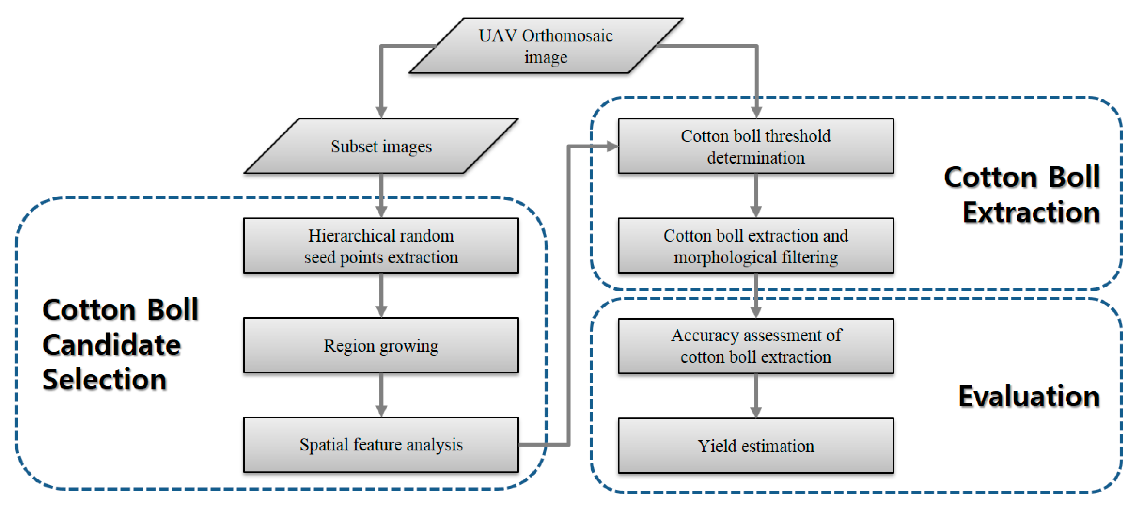
The proposed methodology consists of three parts: (1) cotton boll candidate selection, (2) cotton boll extraction, and (3) the evaluation of the cotton boll extraction results and yield estimation (Figure 1). First, subset images of an UAV orthomosaic image were generated for the initial estimation of cotton boll characteristics. Analyzing subset images is more efficient because the UAV orthomosaic image contains a considerable amount of data compared with other remote sensing data. Random seed points were extracted on each subset image and a region growing algorithm was applied to determine if the generated segments are cotton boll candidates. The spectral information of cotton boll candidates was collected and the brightness threshold values to differentiate cotton bolls from other classes were automatically determined by the Otsu method [36]. Finally, a binary cotton boll image classification was performed by applying the derived threshold values to the UAV orthomosaic image. Two different ways to evaluate the performance of the proposed method were considered in this study: (1) assessing the accuracy of the binary cotton boll classification, and (2) analyzing the cotton yield prediction power by regressing extracted cotton boll features and actual harvested yield.
2.1. Cotton Boll Candidate Selection
Initial seed points of the region growing algorithm were extracted using hierarchical random sampling. We applied 10 iterations, and each iteration extracted 0.1% random pixels of each subset image. Although the number of seed pixels is eventually equal to 1% of the pixels of each subset image, this hierarchical random sampling contributes significantly to reducing computation time. Once the region growing segments located in non-target areas (i.e., background) such as soil and agricultural roads were detected, those regions were masked out for the remaining iterations. Without the hierarchical random sampling, it would waste a lot of time to generate the same region growing segments whenever initial seeds are located on non-target features. This can become a significant computational bottleneck, especially since UAV data results in a larger number of pixels to process when compared to other remote sensing data.
A region growing algorithm was adopted to generate homogeneous segments and to analyze their spatial features from the hierarchically extracted seeds. The region growing algorithm starts from one initial seed and searches neighboring pixels in horizontal, vertical, and diagonal directions based on the spectral similarity of multispectral brightness vectors. Every neighboring pixel that has a similar spectral signature becomes a new seed point and the process repeats itself until there are no more seeds. After the region growing process, spatial features of each segment such as size and roundness were measured to determine if the segment represents either a cotton boll candidate or background. The spectral similarity threshold value for the region growing was determined as 10% of the difference between maximum and minimum pixel values in all band images. Segments bigger than 9 m2 () were marked as a masking area in every iteration. The masking process increases computational efficiency by skipping region growing computation when random seeds fall within already masked areas. For the cotton boll candidate selection, the range of cotton boll sizes was limited to 9 cm2 () and 225 cm2 (), considering that multiple cotton bolls can be neighboring each other in the nadir view orthomosaic image. Segments smaller than 9 cm2 () were regarded as speckle noises and were excluded. In addition, the segments with a roundness index higher than 0.7 () were regarded as cotton boll candidates. Roundness index () was calculated using segment area size () and perimeter () as shown in Equation (1):
which has a value between 0 and 1. A roundness value of 1 represents a perfect circle. The parameters were set to select cotton boll candidate segments which are small and round. We tried to set intuitive and actual size-based criteria so that the criteria could be adjusted considering the images with different spatial resolutions. Additionally, the spectral information of cotton bolls can be inferred adaptively based on the extracted cotton boll candidates in input images, regardless of radiometric and illumination differences in different images. The parameters used in the cotton boll candidate selection are summarized in Table 1.
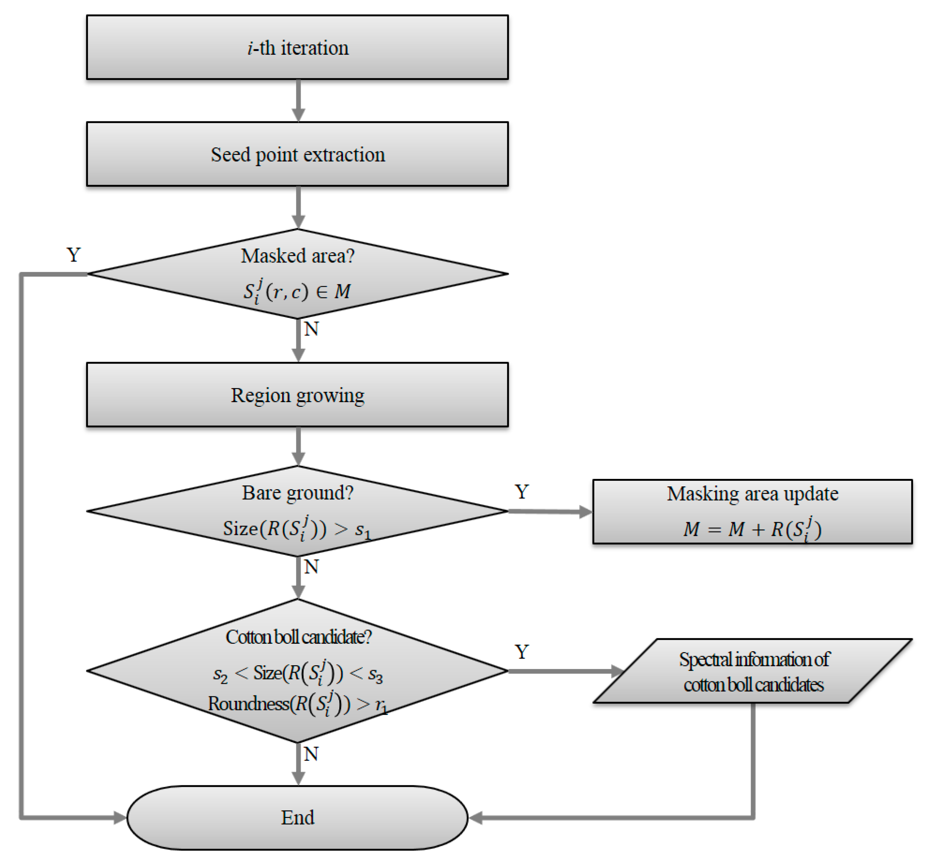
The workflow proposed for the cotton boll candidate selection is shown in Figure 2. In this figure, is the -th seed point in the -th iteration having two-dimensional row () and column () coordinates. is the region growing segment from the seed point , and is the masked area, which represents background classes such as bare ground and other large homogeneous areas. Seed points were randomly generated in every iteration, and only if the seeds do not belong to masked area was the region growing task performed, for computational efficiency. After the region growing task was completed, the background segments were masked out and accumulated for the remaining iterations. Cotton boll candidates were then screened based on size and roundness constraints (Table 1). Finally, the spectral information of each cotton boll candidate was collected over all iterations.
2.2. Cotton Boll Extraction
The cotton boll candidates identified in the previous step represent small and round segments in the subset UAV images. These may include open cotton bolls as well as shadows, leaves, and other small and round objects. The spectral distribution of cotton boll candidates was analyzed in order to distinguish between cotton bolls and other non-target objects. We assumed that cotton bolls have higher spectral values and adopted the Otsu method, which is an automatic thresholding algorithm. This method defines the threshold value in order to maximize class separability between in-class variance () and inter-class variance (). Total variance () can be divided into in-class variance and inter-class variance, as shown in Equation (2), and in-class variance is a weighted sum of each class variance, as shown in Equation (3):
where is the total standard deviation, and are the standard deviations of in- and inter-class, is the threshold value, and are the weights of class 1 and 2, and are the standard deviations of classes 1 and 2. The variances of classes 1 and 2 vary according to the threshold value. The optimized threshold value is determined in order to minimize in-class variance while maximizing inter-class variance. In this study, classes 1 and 2 correspond to open cotton bolls and other non-target objects, respectively.
There is a simple way to set the threshold value empirically to classify open cotton bolls. However, the radiometric characteristics of UAV images vary significantly depending on weather conditions, sensors, and the timing of the flight. It is not practical, then, to set threshold values by manually inspecting orthomosaic images. The main advantage of the proposed method is to automatically determine a threshold value based on the cotton boll candidates such that it can be applied to different images adaptively, without manually adjusting threshold values. Once the threshold was determined from the subset images, values were used to perform a binary classification of cotton bolls on the orthomosaic image. Pixels whose spectral values were greater than the chosen threshold values in each band were classified as cotton bolls. Finally, morphological filtering was applied to filter out speckle noises and relatively big patches using the same size constraints (, ) that were used for the spatial feature analysis of cotton boll candidates.
3. Study Area and Data
3.1. Study Area
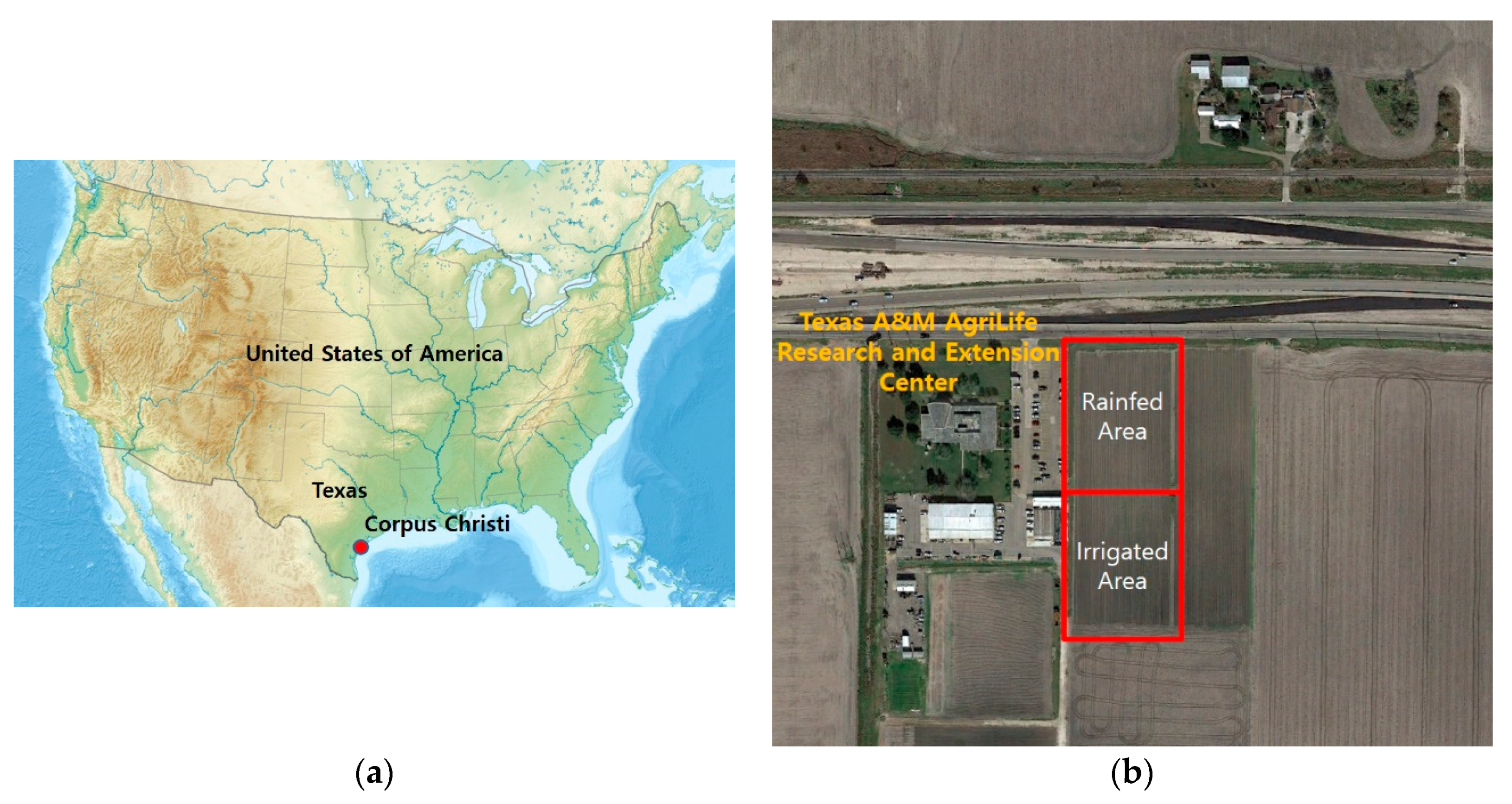
The study area is located at Texas A&M AgriLife Research and Extension Center at Corpus Christi, Texas in the United States (Figure 3). Cotton production is an important economic factor in the United States as the country leads worldwide cotton exportation. Texas produces more cotton than any other state in the United States, and cotton is the leading cash crop in Texas, corresponding to 25% of the country’s cotton production [37]. The experiment contained 31 cotton varieties with two different irrigation regimes: irrigated and rainfed. Each irrigation regime consists of 490 field management grids (7 rows and 70 columns each). Each grid is about 0.96 m by 10 m size and has 10 plants (one plant per 1 m in a north–south direction) with single variety. The study site was exposed to a hot (32 °C on average) and humid (76% on average) climate with average monthly rainfall ranging 50 mm and 90 mm during the season. The study site is suitable to verify the proposed method as it reflects various cotton conditions in terms of variety and irrigation status.
3.2. UAV Data
A DJI Phantom 4 with integrated RGB sensor was used to collect UAV data. Data were acquired on 18 August 2016. An autonomous flight mission was designed with the following conditions: 15 m above-ground altitude, 85% forward overlap, and 85% side overlap, which resulted in a total of 1056 raw images over the study area. Sixteen ground control points (GCPs) were installed in the study area and were surveyed using a survey-grade global positioning system (GPS) unit. Twelve high-quality GCPs out of the total of GCPs were used in the post-processing step to generate precise geospatial data products such as orthomosaic images and a digital elevation model (DEM). An orthorectified image was generated from the raw images using Agisoft Photoscan Pro software [38]. The used functions and parameters are as follows: align photo (high accuracy, reference pair selection), build mesh (arbitrary surface type, medium face count), GCP marker generation and optimization, build dense cloud (high quality, mild depth filtering mode), build DEM (dense cloud source data), and build orthomosaic (DEM surface). The spatial resolution of the resulting orthomosaic image was 0.6 cm with a 0.43-pixel error.
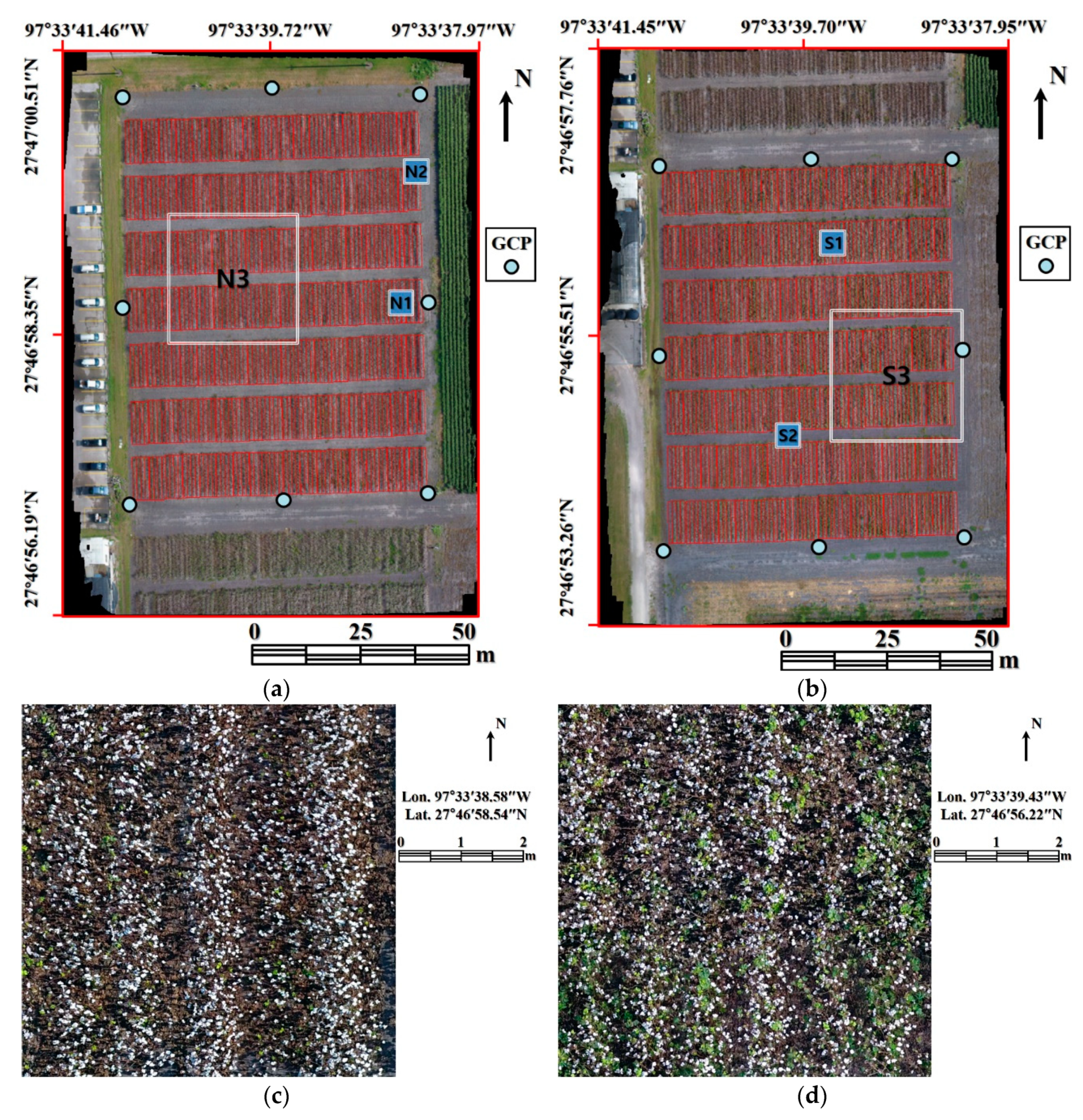
Figure 4a,b show rainfed (north) and irrigated (south) orthomosaic images with plot boundary grids shown as red polygons. Field-harvested yield data were collected for each grid. The north and south orthomosaic images are 16,426 pixels by 22,321 pixels and 16,037 pixels by 22,645 pixels, respectively, which corresponds to 97 m by 137 m and 97 m by 132 m, respectively. The cotton boll area and harvested yield data for each grid (490 grids for each irrigation regime, 9.61 m2 each) were used in the yield estimation analysis.
Two subset images in each irrigation condition were generated for computationally-efficient cotton boll candidate selection. Subset images were manually selected from the middle and edge of a field so that the proposed hierarchical random seed extraction and bare ground masking method could be tested (Figure 4c–f). All subset images are 1000 pixels by 1000 pixels and represent an area of 6 m by 6 m. The subset images, north 1 (N1) and 2 (N2), south 1 (S1) and 2 (S2), are marked in their orthomosaic images (Figure 4a,b). In addition, the accuracy of cotton boll extraction was tested using the north 3 (N3) and south 3 (S3) subset images, 5000 pixels by 5000 pixels (30 m by 30 m area), and they are also marked in orthomosaic images (Figure 4a,b).
3.3. Evaluation
One thousand evaluation pixels (500 cotton bolls and 500 non-cotton bolls) were randomly selected and visually inspected to assess the accuracy of the binary classification. Sampling without weighting results in non-cotton pixels being dominant in the validation dataset and will bias the accuracy assessment results. Pixels in the validation datasets were classified into four categories according to the classification results and their actual classes, as in an error matrix (Table 2). The ‘true positive’ and ‘true negative’ sections include correctly classified pixels, and ‘false positive’ and ‘false negative’ indicate commission and omission errors, respectively. Based on the error matrix, we evaluated the proposed cotton boll classification accuracy. The overall accuracy of the proposed method is the ratio between the sum of ‘true positive’ and ‘true negative’ pixels and the total number of pixels in the validation dataset. In addition to the overall accuracy, other accuracy measures such as precision, recall, F-measure, and the Jaccard coefficient were adopted. Precision and recall are accuracy measurements considering commission and omission errors, respectively. F-measure is the harmonic mean of precision and recall. The Jaccard coefficient is a measure of asymmetric information on binary classification and solely focuses on the target class (cotton bolls); therefore, it is less biased by the classification accuracy of the non-target class (others). All accuracy measurements are shown in Equations (4)–(7):
These accuracy measures can range between 0 and 1, where 1 represents perfect cotton boll detection, and 0 indicates failure.
The proposed method was designed to extract open cotton boll pixels from orthomosaic images, such that the open boll extraction results can be used to predict crop yield. In addition to the classification accuracy assessment, open cotton boll detection results were correlated with field-harvested yield data. For the yield estimation analysis, we generated GIS plot grids that match with field management units and were used to calculate the sum of the open cotton boll area within each grid. The sum of the open cotton boll area was used as an independent variable and field-harvested yield was used as a dependent variable to perform a linear regression analysis. Pearson’s correlation coefficient and R2 were calculated to assess the regression results. For the linear regression analysis, we used 70% of the total GIS grids as training data and the rest of the grids were used as validation data. The predicted and field-harvested yields were compared using root mean square error.
4. Results
4.1. Cotton Boll Candidate Selection
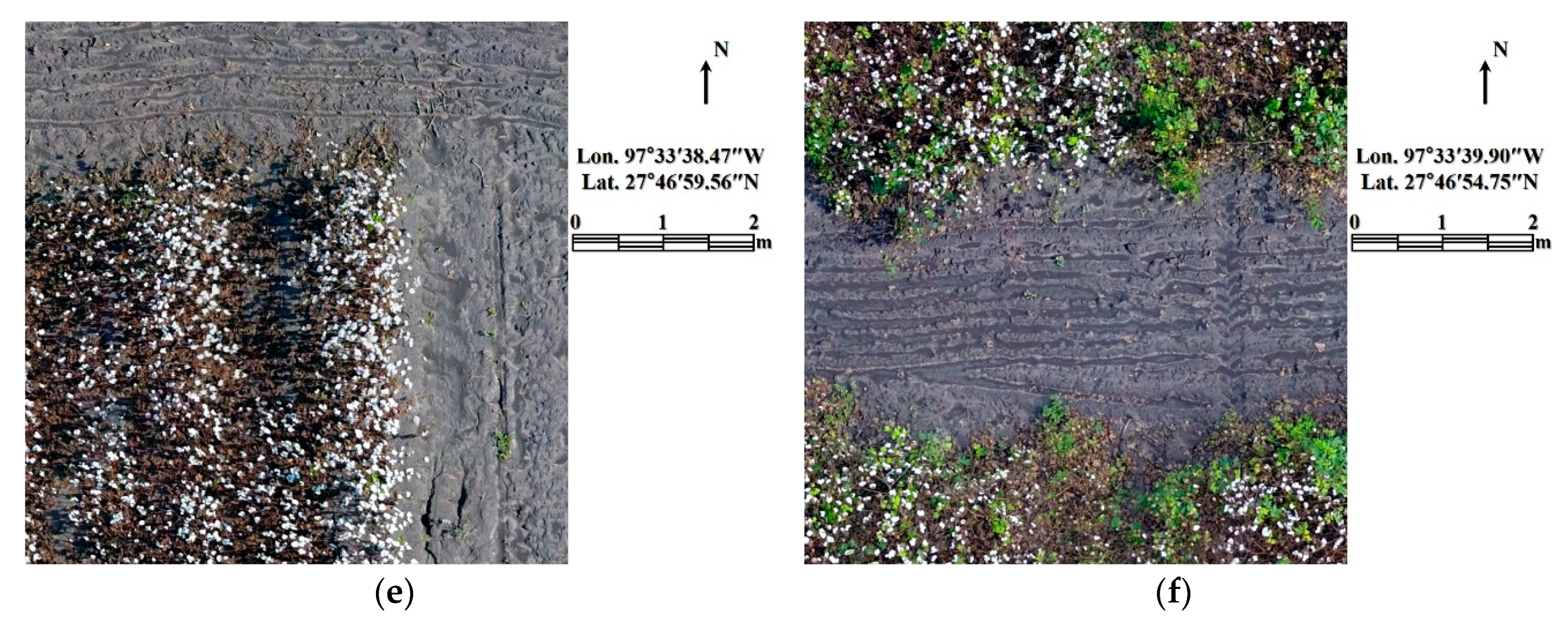
Cotton boll candidate selection was performed to obtain robust spectral information about cotton bolls without ground reference data or manual interpretation so that the spectral information of cotton bolls could be determined objectively and adjusted based on the spectral conditions of input images. We adopted a hierarchical random sampling approach to speed up the region growing process when compared with a traditional approach that uses the same number of seed points. We tested the proposed sampling approach with the subset images containing bare ground (N2 and S2). The computation times of the proposed method and the traditional sampling approach were 454 s and 12,721 s, and 330 s and 17,311 s, in the north (N2) and south (S2) sites, respectively. The computation time was measured using a program written in Matlab R2013 on a workstation with an i7 3.40 GHz CPU and 16 GB of RAM. The final masked area is shown in Figure 5. The N1 and S1 subset images contained no masked-out areas because they only included crop area within the boundary grids (Figure 5a,b). In contrast, a significant amount of area was masked out in the N2 and S2 subset images (Figure 5c,d) since they included background regions such as bare ground. The proposed hierarchical region growing process resulted in a 38-fold increase in computational efficiency when compared to a traditional method.
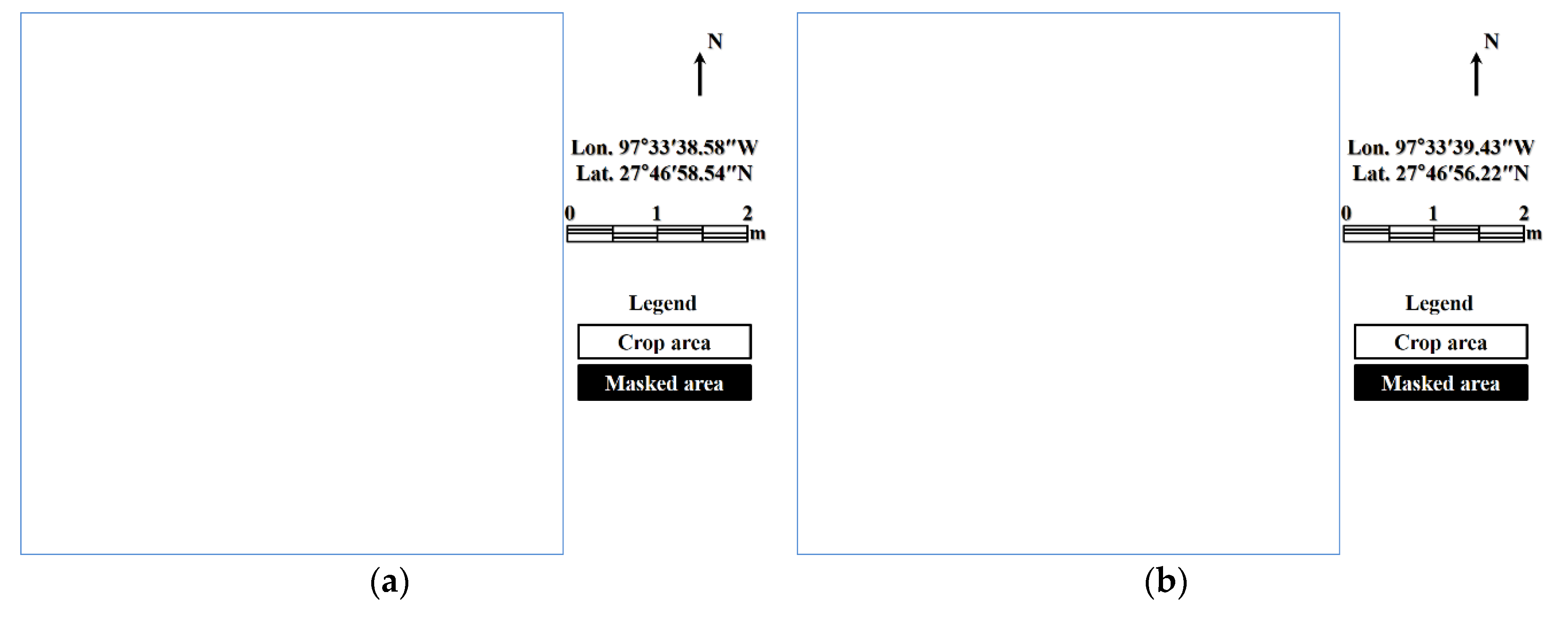
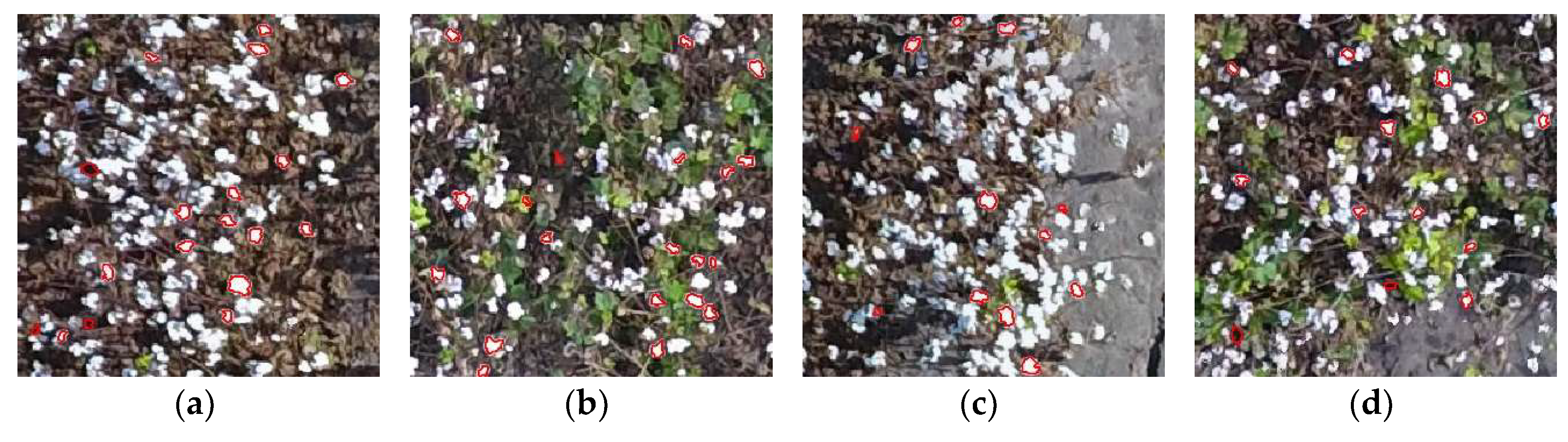
The size and shape constraints (, , and ) of the cotton boll candidate selection process were designed to extract segments that are highly likely to be cotton bolls. As orthomosaic images often contain connected cotton bolls with irregular shape due to nadir view, the roundness constraint was used to separate out single cotton bolls and extract relevant spectral information of the cotton boll candidates (Figure 6). The number of detected cotton boll candidates in N1, S1, N2, and S2 were 172, 184, 83, and 94, respectively.
4.2. Cotton Boll Extraction
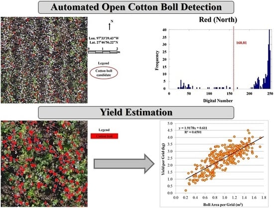
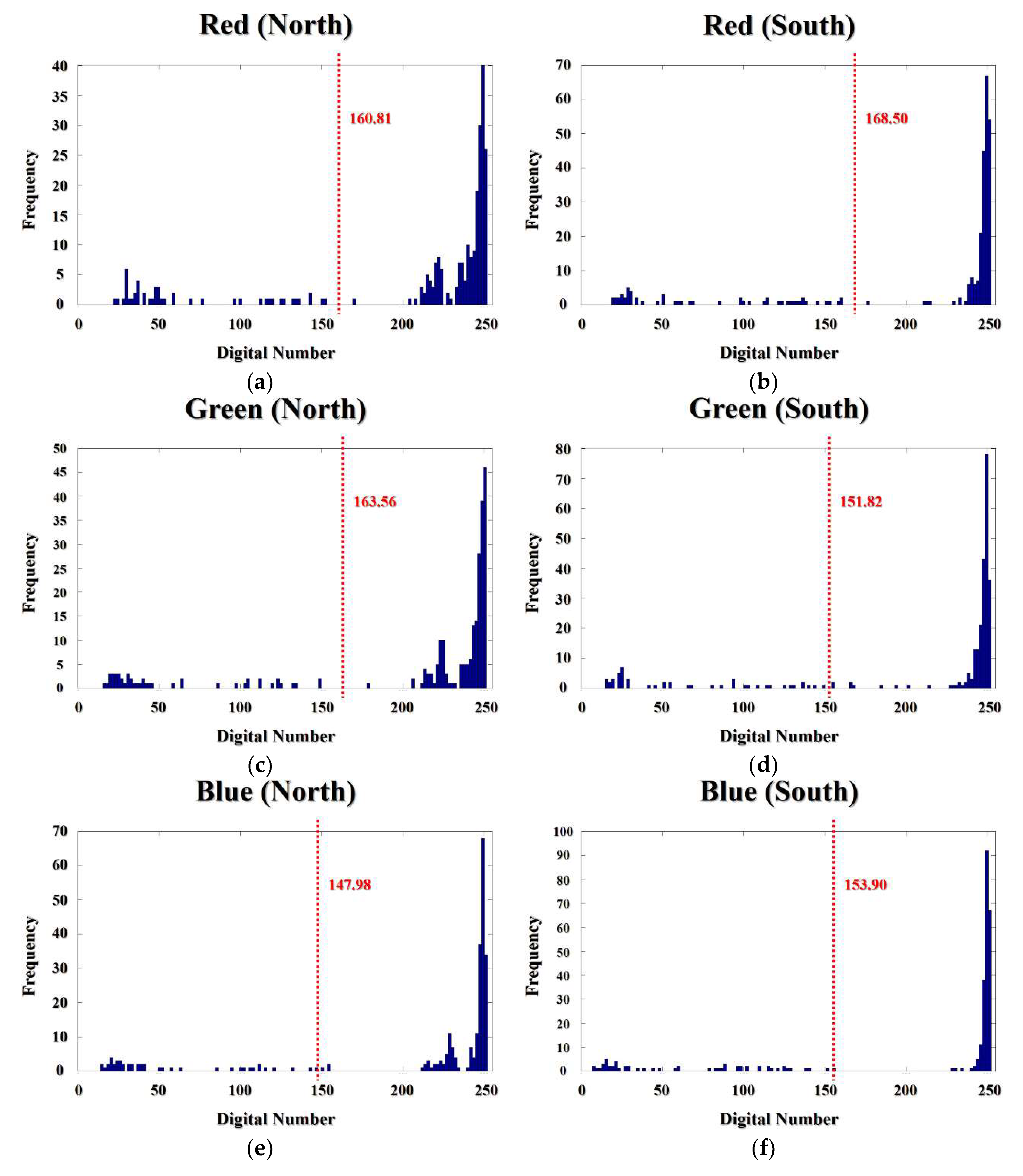
The cotton boll extraction process uses spectral information of the cotton boll candidates to automatically calculate threshold values that separate cotton bolls from other non-target objects. The histograms of red, green, and blue bands in both sites are shown in Figure 7. All histograms have a similar bi-modal distribution shape; i.e., high frequency bins concentrated in narrow high digital numbers (>200) and low frequency bins widely spread over low digital numbers (<200). Most of the extracted cotton boll candidates correctly resulted from actual cotton bolls, which contributed to the high frequency bins in high digital numbers. Conversely, cotton boll candidates resulted from non-cotton boll segments such as shadows, branches, leaves, and isolated spots on the ground contributing to low frequency bins in low digital numbers. The Otsu automatic thresholding method was adopted to automatically determine brightness threshold values that separate these two dominant distributions, because the Otsu method assumes bi-modal distribution.
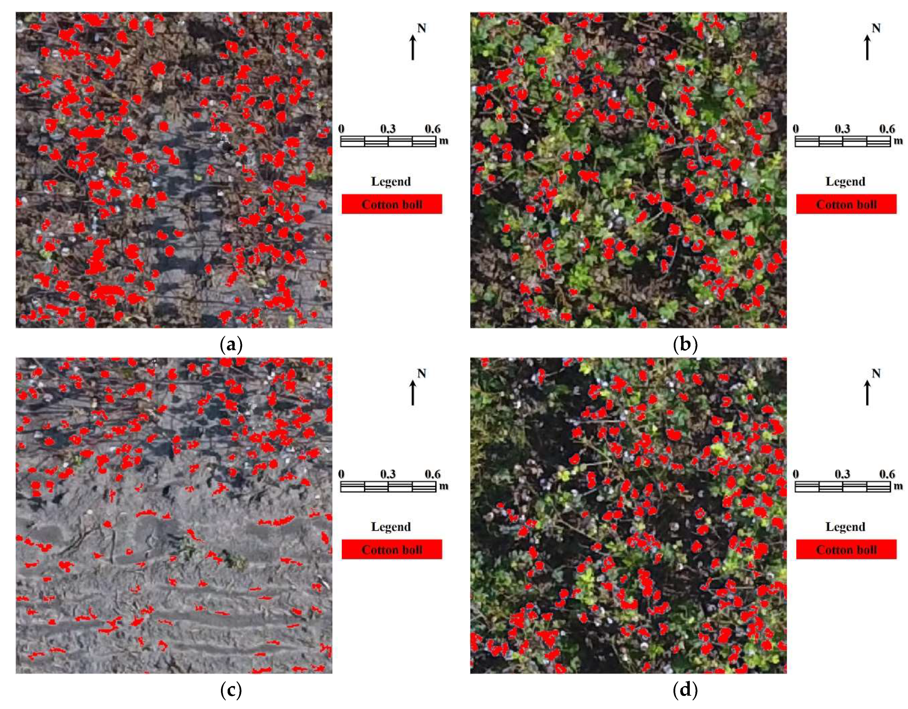
The automatically calculated threshold values of red, green, and blue bands using the proposed approach were 160.81, 163.56, and 147.98 for the north site and 168.50, 151.82, and 153.90 for the south site, respectively. These threshold values were then applied to the orthomosaic images from each site to finalize the cotton boll extraction procedure. Pixels with higher digital numbers than the threshold values in each band were classified as cotton bolls. In addition, the size constraints (, ) were applied to the binary classification results for noise reduction. The roundness constraint () was not used in this step because cotton bolls on the upper and lower canopy look as if they are connected in orthomosaic images due to the nadir view. Cotton boll extraction results for subsets N3 and S3 of the north and south sites are shown in Figure 8.
4.3. Accuracy Assessment
The cotton boll extraction results were evaluated using an error matrix. Pixels were randomly selected from the orthomosaic images and visually inspected to generate reference data. Five hundred reference pixels for each class (cotton bolls and other non-target objects) were used because the evaluation in binary classification can be easily biased by the dominant class; non-cotton boll pixels in this case. The accuracy assessment results of the proposed approach when applied to the N3 and S3 test images are shown in Table 3 and Table 4. Parameters used to assess accuracy (precision, recall, F-measure, and Jaccard coefficient) showed high accuracies, ranging from 88% to 97%. Precision and the Jaccard coefficient in the north site were about 4% lower than those of the south site. This is because a higher number of non-cotton boll pixels were classified as cotton bolls in the north site due to bright bare soil (i.e., false positives).
The cotton boll extraction results were correlated with the actual harvested yield data. The main advantage of the proposed approach is to automatically extract cotton bolls from UAV data, for a direct estimation of crop productivity or yield. For the correlation analysis, GIS plot boundaries were used to calculate the sum of cotton boll area within each plot. Pearson correlation coefficients between the cotton boll area and harvested yield in the north and south sites were 0.81 and 0.79, respectively, indicating a strong positive correlation.
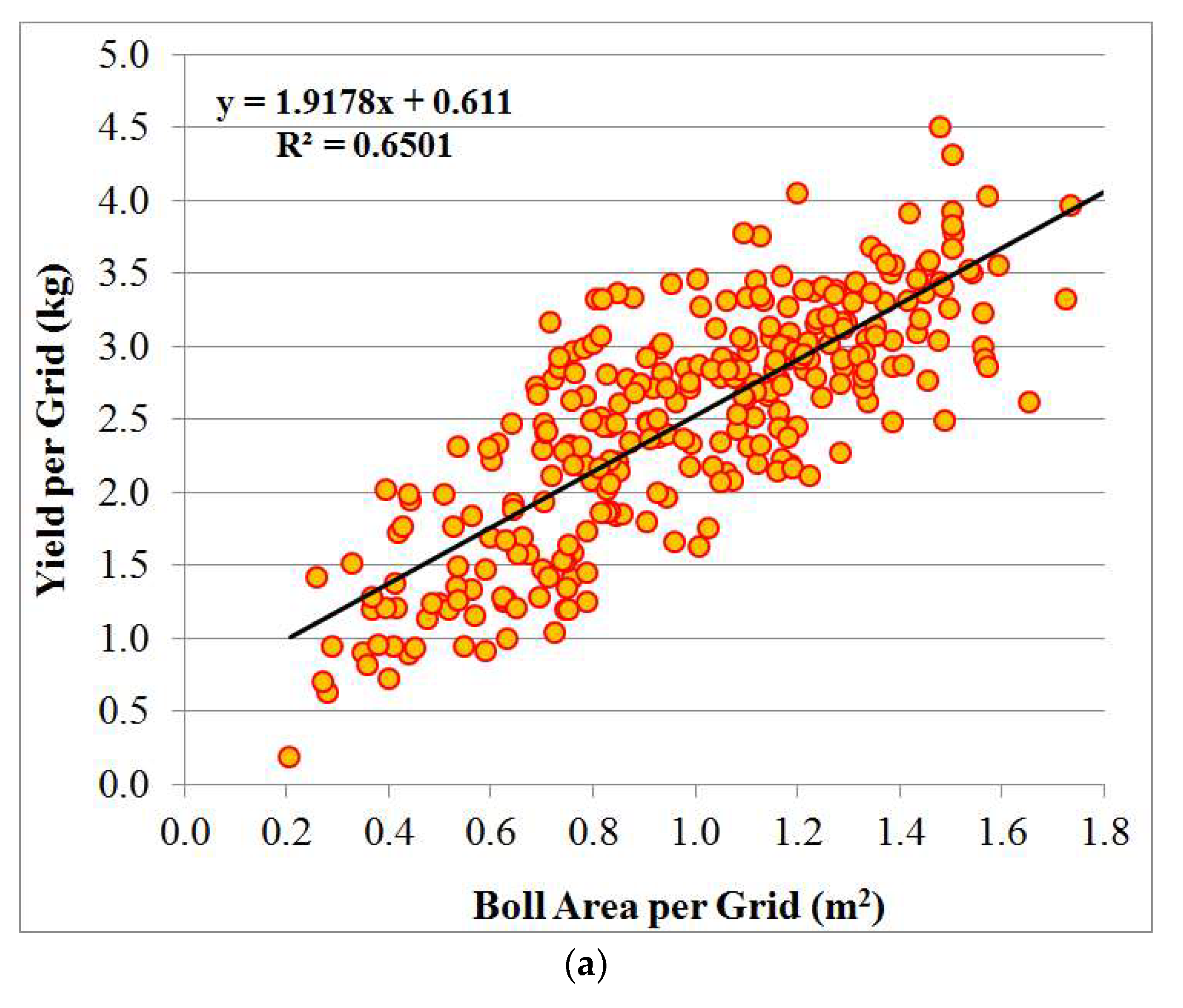
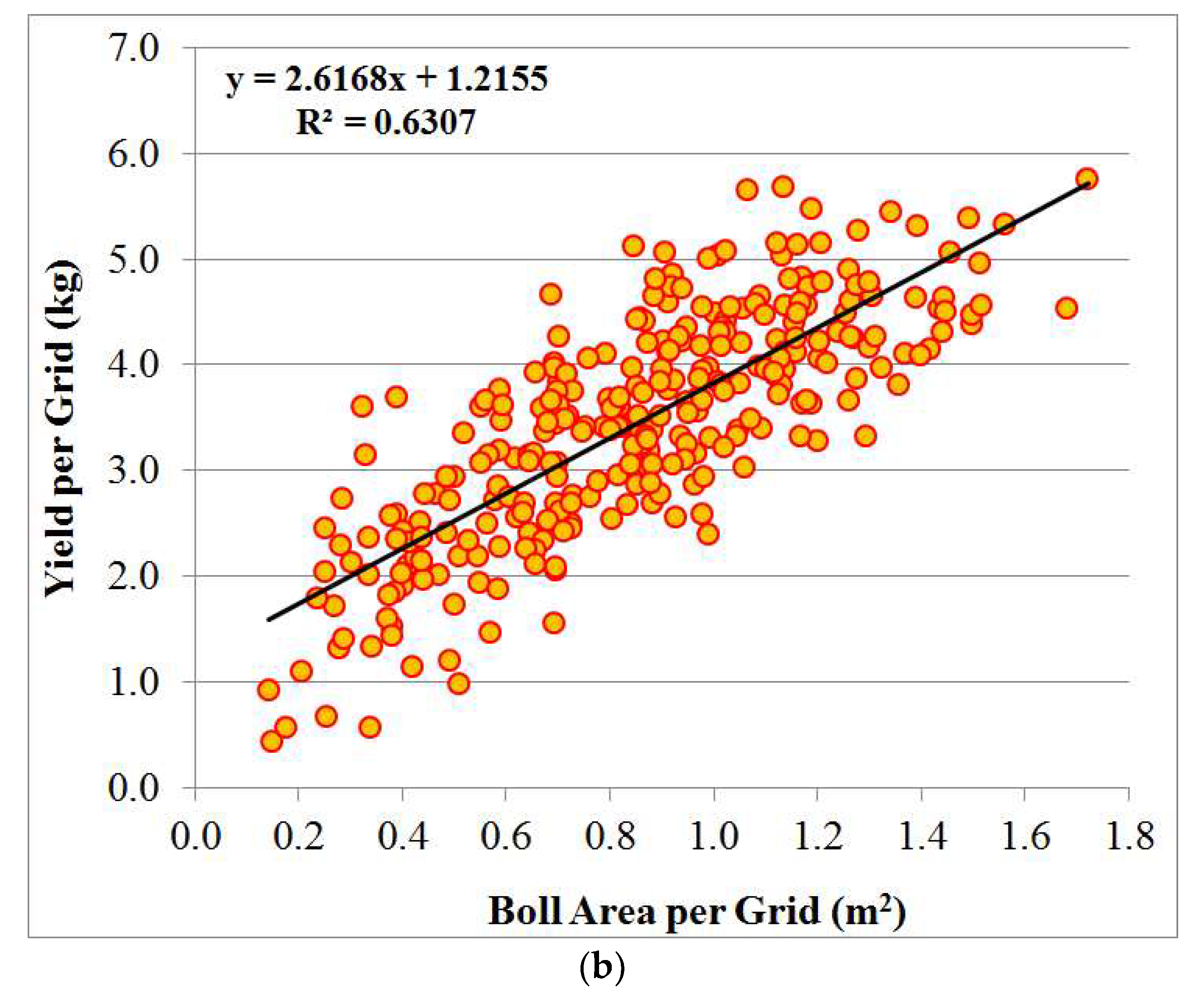
Linear regression analysis between boll area and harvested yield data was conducted using 70% of grids as training data. The north and south sites were analyzed separately because linear regression parameters, slope and offset, may vary depending on the irrigation treatment (e.g., rainfed and irrigated). As shown in Figure 9, R2 values for each site were similar. Although we only used a single input variable, i.e., automatically calculated cotton boll area, R2 values showed adequate estimating performance at 0.65 and 0.63 for the north and south sites, respectively [39].
5. Discussion
5.1. Cotton Boll Candidate Selection and Cotton Boll Extraction
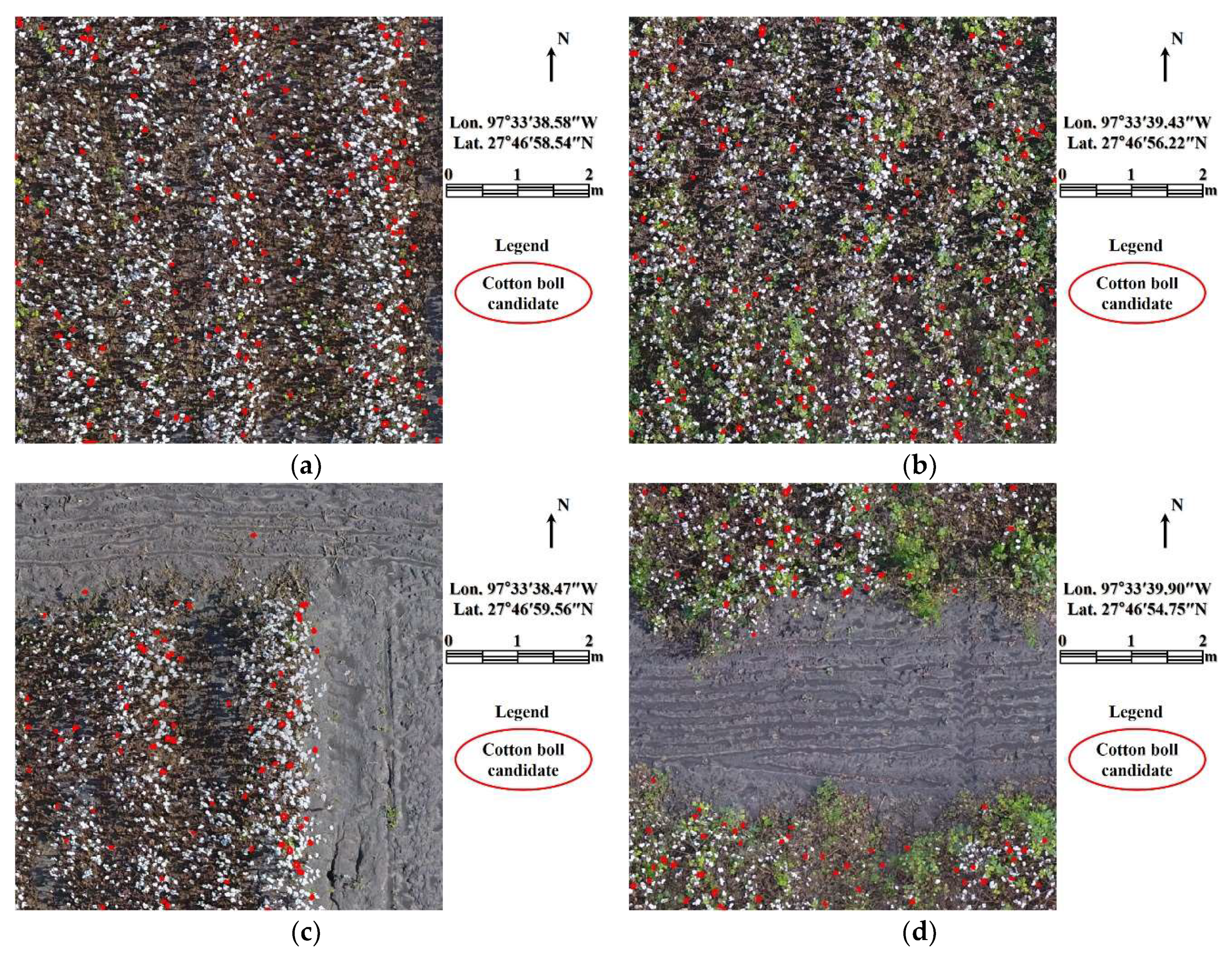
The spectral similarity of the region growing process was set as 10% of the maximum and minimum digital number range of input images, which is a commonly used value. The roundness criterion was empirically determined as 0.7. Basically, the threshold values for the cotton boll candidate selection were derived from the spectral values of input images. Therefore, the threshold values can be adaptively determined and data acquisition at a different date rarely affects the proposed cotton boll candidate selection. However, cm-level spatial resolution is required to detect small cotton boll candidates. In the case of low-resolution images (>1~2 cm), cotton boll candidates would be represented by several pixels, which results in confusion with noises and inaccurate calculation of the roundness index. Most of the cotton boll candidates were correctly located, but there were some non-cotton segments identified as cotton boll candidates because of shadows, branches, leaves, and isolated spots on the ground (Figure 10a,d). Both sites on the south side (S1 and S2) contained more green leaves due to the irrigation treatment; however, the proposed cotton boll candidate selection process was not significantly affected.
The proposed method accurately extracted cotton bolls based on automatically derived threshold values and the morphological filtering process. Although most pixels classified as cotton bolls were actual cotton bolls (Figure 11a,b), the proposed approach also suffered from commission and omission errors. The commission errors were mainly caused by isolated bright spots on the ground that did not meet the noise removal constraints (Figure 11c). These commission errors were more frequent in the north site because rainfed land has brighter soil than irrigated land. The omission errors were mainly caused by shadows since cotton bolls located in the lower canopy are usually shadowed by the upper canopy, and they have relatively low digital numbers compared to the cotton bolls on the upper canopy (Figure 11d).
5.2. Accuracy Assessment
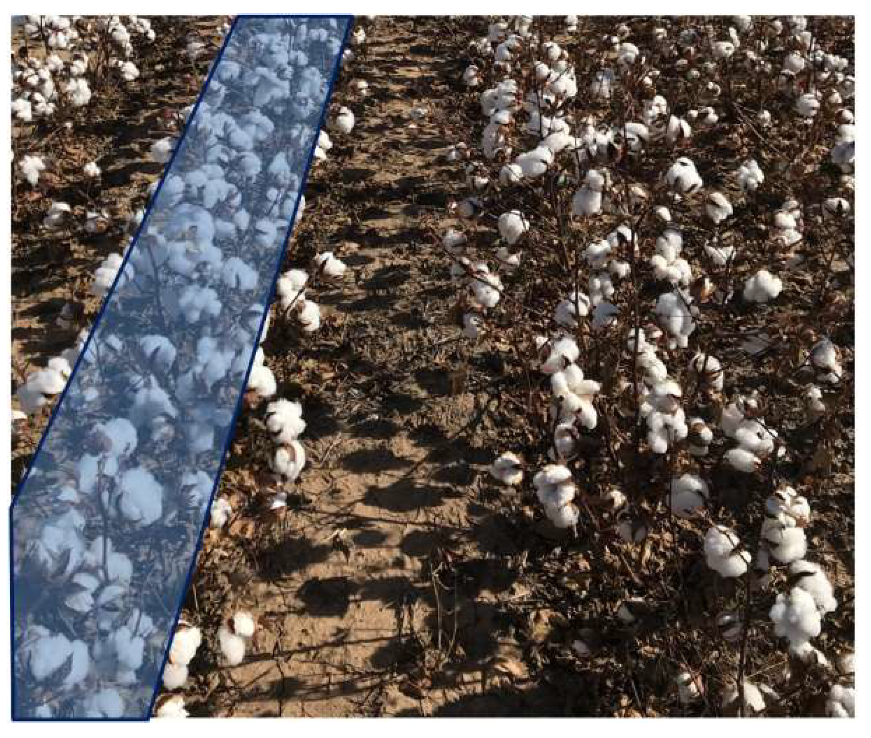
The average harvested yield per plot grid was 2.53 kg and 3.48 kg for the north and south sites, respectively. Although the irrigated site (south) had higher harvested yield, the summarized boll area per plot grid for the south site is smaller (0.86 m2) than the north site (1.00 m2). In addition, the average number of cotton bolls per grid in the south site (304) is fewer than the north site (337). The underestimation of cotton boll area in the south site is mainly caused by hidden or shadowed cotton bolls on the lower canopy due to remained leaves. This is the reason why the regression parameters (slope and offset) of the south site had larger values, resulting in higher yield estimation for a given input boll area value. This indicates that crop defoliation effectiveness affects the performance of the cotton boll area-based yield estimation. In addition, the cotton yield estimation parameters vary depending not only on irrigation status (presence of leaves) but also varieties, because the distributions of cotton bolls on the upper and lower canopy are different by varieties, which affects the amount of occlusion of the lower canopy in orthomosaic images (Figure 12). Therefore, the study site includes different irrigation statuses (to analyze the effect of defoliation), and 31 cotton varieties (to acquire general yield estimation parameters) were chosen. In this study, it was assumed that the cotton boll area which can be detected from nadir view image is basically proportional to the total cotton bolls. Therefore, although some parts of the lower canopy were not captured in the orthomosaic images, the occlusion effect of the lower canopy was compensated in the linear yield estimation models. The regression models for yield estimation were tested and the root mean square errors (RMSEs) were 0.47 kg and 0.66 kg in the north and south site, respectively, when models were applied to the remaining 30% validation grids. The RMSEs correspond to 19% of the average harvested yield for both sites.
As an alternative way to estimate cotton yield in early season, yield estimation models using plant covered area, plant height, plant volume, or NDVI can be utilized. However, this approach needs different kinds of data and mostly requires time-series data, because crops are growing. It is difficult to select the best data for yield estimation considering the changing environmental conditions and growing crops. On the contrary, although the proposed method uses late phase data, it requires only one kind of data (cotton boll area) for yield estimation which means that it is simple, cost-effective, and enables intuitive explanation (directly from cotton bolls to yield).
6. Conclusions
In this study, we propose an automatic open cotton boll extraction method. It uses a hierarchical region growing process to improve computational efficiency so that it can be applied to very high-resolution UAV images effectively. Spatial information of region growing segments was used to determine cotton boll candidates. The threshold values that automatically separate cotton bolls from other non-cotton objects were derived based on subset input images for adaptive application. The proposed method utilizes unsupervised procedures to determine threshold values and can be applied to a single-date images without any training data. In addition, we verified the possibility of extracting open cotton bolls using UAV images for yield estimation. According to the accuracy assessment results of the cotton boll classification, cotton bolls which are directly related with actual yield were extracted with high accuracy (>88%). The extracted cotton boll area and harvested yield showed a strong positive correlation (0.8). A linear regression model to estimate yield using a single variable (i.e., cotton boll area) was developed with R2 values around 0.64. The proposed method is a novel approach that enables the extraction of specific regions of interest from UAV images in an automated and unsupervised way.
The proposed method has limitations linked to data characteristics. Cotton boll area tend to be underestimated because lower canopy cotton bolls cannot be seen in orthomosaic images. Excessive wind will cause distortions in orthomosaic images and affect cotton boll detection accuracy. In order to improve the proposed method, raw image-based cotton boll extraction and its direct geo-referencing are currently being investigated. Raw images contain lower canopy cotton bolls, due to their oblique view characteristics, and have no distortion, which is generally an issue in the orthorectification process.
Author Contributions
Formal analysis, J.Y.; Investigation, J.Y.; Methodology, J.Y.; Project administration, J.L.; Resources, J.J., A.C., M.M.M. and J.L.; Validation, J.Y.; Visualization, J.Y.; Writing—original draft, J.Y.; Writing—review & editing, J.J. and M.M.M.
Funding
This research was supported by Basic Science Research Program through the National Research Foundation of Korea(NRF) funded by the Ministry of Education(2017R1A6A3A03005183).
Acknowledgments
This work was supported by Texas A&M AgriLife Research.
Conflicts of Interest
The authors declare no conflict of interest.
References
- Jiang, Z.; Chen, Z.; Chen, J.; Ren, J.; Li, Z.; Sun, L. The estimation of regional crop yield using ensemble-based four-dimensional variational data assimilation. Remote Sens. 2014, 6, 2664–2681. [Google Scholar] [CrossRef]
- Bellón, B.; Bégué, A.; Lo Seen, D.; de Almeida, C.A.; Simões, M. A remote sensing approach for regional-scale mapping of agricultural land-use systems based on NDVI time series. Remote Sens. 2017, 9, 600. [Google Scholar] [CrossRef]
- Arvor, D.; Jonathan, M.; Meirelles, M.S.P.; Dubreuil, V.; Durieux, L. Classification of MODIS EVI time series for crop mapping in the state of Mato Grosso, Brazil. Int. J. Remote Sens. 2011, 32, 7847–7871. [Google Scholar] [CrossRef]
- Rembold, F.; Atzberger, C.; Savin, I.; Rojas, O. Using low resolution satellite imagery for yield prediction and yield anomaly detection. Remote Sens. 2013, 5, 1704–1733. [Google Scholar] [CrossRef] [Green Version]
- Zhang, M.; Wu, B.; Yu, M.; Zou, W.; Zheng, Y. Crop condition assessment with adjusted NDVI using the uncropped arable land ratio. Remote Sens. 2014, 6, 5774–5794. [Google Scholar] [CrossRef]
- Simms, D.M.; Waine, T.W.; Taylor, J.C.; Juniper, G.R. The application of time-series MODIS NDVI profiles for the acquisition of crop information across Afghanistan. Int. J. Remote Sens. 2014, 35, 6234–6254. [Google Scholar] [CrossRef]
- Wardlow, B.D.; Egbert, S.L. A comparison of MODIS 250-m EVI and NDVI data for crop mapping: A case study for southwest Kansas. Int. J. Remote Sens. 2010, 31, 805–830. [Google Scholar] [CrossRef]
- Akbari, M.; Mamanpoush, A.R.; Gieske, A.; Miranzadeh, M.; Torabi, M.; Salemi, H.R. Crop and land cover classification in Iran using Landsat 7 imagery. Int. J. Remote Sens. 2006, 27, 4117–4135. [Google Scholar] [CrossRef]
- Son, N.T.; Chen, C.F.; Chen, C.R.; Duc, H.N.; Chang, L.Y. A phenology-based classification of time-series MODIS data for rice crop monitoring in Mekong Delta, Vietnam. Remote Sens. 2013, 6, 135–156. [Google Scholar] [CrossRef]
- Bocco, M.; Sayago, S.; Willington, E. Neural network and crop residue index multiband models for estimating crop residue cover from Landsat TM and ETM+ images. Int. J. Remote Sens. 2014, 35, 3651–3663. [Google Scholar] [CrossRef]
- Rao, N.R. Development of a crop-specific spectral library and discrimination of various agricultural crop varieties using hyperspectral imagery. Int. J. Remote Sens. 2008, 29, 131–144. [Google Scholar] [CrossRef]
- Potgieter, A.; Apan, A.; Hammer, G.; Dunn, P. Estimating winter crop area across seasons and regions using time-sequential MODIS imagery. Int. J. Remote Sens. 2011, 32, 4281–4310. [Google Scholar] [CrossRef] [Green Version]
- Esquerdo, J.C.D.M.; Zullo Júnior, J.; Antunes, J.F.G. Use of NDVI/AVHRR time-series profiles for soybean crop monitoring in Brazil. Int. J. Remote Sens. 2011, 32, 3711–3727. [Google Scholar] [CrossRef]
- Zheng, Y.; Zhang, M.; Zhang, X.; Zeng, H.; Wu, B. Mapping winter wheat biomass and yield using time series data blended from PROBA-V 100- and 300-m S1 products. Remote Sens. 2016, 8, 824. [Google Scholar] [CrossRef]
- Sakamoto, T.; Wardlow, B.D.; Gitelson, A.A. Detecting spatiotemporal changes of corn developmental stages in the US corn belt using MODIS WDRVI data. IEEE Trans. Geosci. Remote Sens. 2011, 49, 1926–1936. [Google Scholar] [CrossRef]
- Meroni, M.; Fasbender, D.; Balaghi, R.; Dali, M.; Haffani, M.; Haythem, I.; Hooker, J.; Lahlou, M.; Lopez-Lozano, R.; Mahyou, H.; et al. Evaluating NDVI data continuity between SPOT-VEGETATION and PROBA-V missions for operational yield forecasting in North African countries. IEEE Trans. Geosci. Remote Sens. 2016, 54, 795–804. [Google Scholar] [CrossRef]
- Hartfield, K.A.; Marsh, S.E.; Kirk, C.D.; Carrière, Y. Contemporary and historical classification of crop types in Arizona. Int. J. Remote Sens. 2013, 34, 6024–6036. [Google Scholar] [CrossRef]
- Huang, J.; Wang, H.; Dai, Q.; Han, D. Analysis of NDVI data for crop identification and yield estimation. IEEE J. Sel. Top. Appl. Earth Observ. Remote Sens. 2014, 7, 4374–4384. [Google Scholar] [CrossRef]
- Zhang, X.; Zhang, M.; Zheng, Y.; Wu, B. Crop mapping using PROBA-V time series data at the Yucheng and Hongxing farm in China. Remote Sens. 2016, 8, 915. [Google Scholar] [CrossRef]
- Fan, C.; Zheng, B.; Myint, S.W.; Aggarwal, R. Characterizing changes in cropping patterns using sequential Landsat imagery: An adaptive threshold approach and application to Phoenix, Arizona. Int. J. Remote Sens. 2014, 35, 7263–7278. [Google Scholar] [CrossRef]
- Li, Q.; Wang, C.; Zhang, B.; Lu, L. Object-based crop classification with Landsat-MODIS enhanced time-series data. Remote Sens. 2015, 7, 16091–16107. [Google Scholar] [CrossRef]
- Murakami, T.; Ogawa, S.; Ishitsuka, N.; Kumagai, K.; Saito, G. Crop discrimination with multitemporal SPOT/HRV data in the Saga Plains, Japan. Int. J. Remote Sens. 2001, 22, 1335–1348. [Google Scholar] [CrossRef]
- De Wit, A.J.W.; Clevers, J.G.P.W. Efficiency and accuracy of per-field classification for operational crop mapping. Int. J. Remote Sens. 2004, 25, 4091–4112. [Google Scholar] [CrossRef]
- Gitelson, A.A.; Viña, A.; Masek, J.G.; Verma, S.B.; Suyker, A.E. Synoptic monitoring of gross primary productivity of maize using Landsat data. IEEE Geosci. Remote Sens. Lett. 2008, 5, 133–137. [Google Scholar] [CrossRef]
- Dubovyk, O.; Menz, G.; Lee, A.; Schellberg, J.; Thonfeld, F.; Khamzina, A. SPOT-based sub-field level monitoring of vegetation cover dynamics: A case of irrigated croplands. Remote Sens. 2015, 7, 6763–6783. [Google Scholar] [CrossRef]
- Inglada, J.; Arias, M.; Tardy, B.; Hagolle, O.; Valero, S.; Morin, D.; Dedieu, G.; Sepulcre, G.; Bontemps, S.; Defourny, P.; et al. Assessment of an operational system for crop type map production using high temporal and spatial resolution satellite optical imagery. Remote Sens. 2015, 7, 12356–12379. [Google Scholar] [CrossRef]
- Marshall, M.T.; Husak, G.J.; Michaelsen, J.; Funk, C.; Pedreros, D.; Adoum, A. Testing a high-resolution satellite interpretation technique for crop area monitoring in developing countries. Int. J. Remote Sens. 2011, 32, 7997–8012. [Google Scholar] [CrossRef]
- Wei, C.; Huang, J.; Mansaray, L.R.; Li, Z.; Liu, W.; Han, J. Estimation and mapping of winter oilseed rape LAI from high spatial resolution satellite data based on a hybrid method. Remote Sens. 2017, 9, 488. [Google Scholar] [CrossRef]
- Coltri, P.P.; Zullo, J.; do Valle Goncalves, R.R.; Romani, L.A.S.; Pinto, H.S. Coffee crop’s biomass and carbon stock estimation with usage of high resolution satellites images. IEEE J. Sel. Top. Appl. Earth Observ. Remote Sens. 2013, 6, 1786–1795. [Google Scholar] [CrossRef]
- Schirrmann, M.; Giebel, A.; Gleiniger, F.; Pflanz, M.; Lentschke, J.; Dammer, K.H. Monitoring agronomic parameters of winter wheat crops with low-cost UAV imagery. Remote Sens. 2016, 8, 706. [Google Scholar] [CrossRef]
- Bendig, J.; Bolten, A.; Bennertz, S.; Broscheit, J.; Eichfuss, S.; Bareth, G. Estimating biomass of barley using crop surface models (CSMs) derived from UAV-based RGB imaging. Remote Sens. 2014, 6, 10395–10412. [Google Scholar] [CrossRef]
- Schirrmann, M.; Hamdorf, A.; Giebel, A.; Gleiniger, F.; Pflanz, M.; Dammer, K.H. Regression kriging for improving crop height models fusing ultra-sonic sensing with UAV imagery. Remote Sens. 2017, 9, 665. [Google Scholar] [CrossRef]
- Torres-Sánchez, J.; López-Granados, F.; Peña, J.M. An automatic object-based method for optimal thresholding in UAV images: Application for vegetation detection in herbaceous crops. Comput. Electron. Agric. 2015, 114, 43–52. [Google Scholar] [CrossRef] [Green Version]
- Peña, J.M.; Torres-Sánchez, J.; De Castro, A.I.; Kelly, M.; López-Granados, F. Weed mapping in early-season maize fields using object-based analysis of unmanned aerial vehicle (UAV) images. PLoS ONE 2013, 8, e77151. [Google Scholar] [CrossRef] [PubMed]
- López-Granados, F.; Torres-Sánchez, J.; De Castro, A.I.; Serrano-Pérez, A.; Mesas-Carrascosa, F.J.; Peña, J.M. Object-based early monitoring of a grass weed in a grass crop using high resolution UAV imagery. Agron. Sustain. Dev. 2016, 36, 67. [Google Scholar] [CrossRef]
- Otsu, N. A threshold selection method from gray-level histograms. IEEE Trans. Syst. Man Cybern. Syst. 1979, 9, 62–66. [Google Scholar] [CrossRef]
- Texas Is Cotton Country. Available online: https://web.archive.org/web/20131021084716/http://cotton.tamu.edu/cottoncountry.htm (accessed on 28 May 2018).
- Agisoft PhotoScan. Available online: http://www.agisoft.com/ (accessed on 28 May 2018).
- Ostertagová, E. Modelling using polynomial regression. Procedia Eng. 2012, 48, 500–506. [Google Scholar] [CrossRef]
Figure 1.
Overall methodology workflow. UAV: unmanned aerial vehicle.

Figure 2.
Cotton boll candidate selection.

Figure 3.
Location of the study area. (a) Corpus Christi, Texas; (b) Texas A&M AgriLife Research and Extension Center (27°46′58.33′′ N, 97°33′43.84′′ W).
Figure 3.
Location of the study area. (a) Corpus Christi, Texas; (b) Texas A&M AgriLife Research and Extension Center (27°46′58.33′′ N, 97°33′43.84′′ W).

Figure 4.
UAV images. (a) orthomosaic image of the rainfed area (north) and accuracy test area (N3); (b) orthomosaic image of the irrigated area (south) and accuracy test area (S3); (c,e) subset images of the rainfed area (N1 and N2); (d,f) subset images of the irrigated area (S1 and S2).
Figure 4.
UAV images. (a) orthomosaic image of the rainfed area (north) and accuracy test area (N3); (b) orthomosaic image of the irrigated area (south) and accuracy test area (S3); (c,e) subset images of the rainfed area (N1 and N2); (d,f) subset images of the irrigated area (S1 and S2).


Figure 5.
Bare ground masking results in subset images. (a) N1; (b) S1; (c) N2; (d) S2.


Figure 6.
Cotton boll candidate extraction. (a) N1; (b) S1; (c) N2; (d) S2.

Figure 7.
Histograms of cotton boll candidates. Red bands of (a) north and (b) south sites; green bands of (c) north and (d) south sites; blue bands of (e) north and (f) south sites.
Figure 7.
Histograms of cotton boll candidates. Red bands of (a) north and (b) south sites; green bands of (c) north and (d) south sites; blue bands of (e) north and (f) south sites.

Figure 8.
Cotton boll extraction results. (a) N3; (b) S3 test sites.

Figure 9.
Linear regression analysis between boll area and harvested yield. (a) north and (b) south sites.
Figure 9.
Linear regression analysis between boll area and harvested yield. (a) north and (b) south sites.


Figure 10.
Enlarged cotton boll candidates. (a) N1; (b) S1; (c) N2; (d) S2.

Figure 11.
Enlarged cotton boll extraction results. (a) N3; (b) S3; (c) commission errors in N3 caused by bright spots on the ground; (d) omission errors in S3 caused by shadowed cotton bolls.
Figure 11.
Enlarged cotton boll extraction results. (a) N3; (b) S3; (c) commission errors in N3 caused by bright spots on the ground; (d) omission errors in S3 caused by shadowed cotton bolls.

Figure 12.
Ground photo of cotton plants and nadir view perspective.


Table 1.
Parameters in cotton boll candidate selection.
| Processing | Parameter | Value |
|---|---|---|
| Hierarchical Random Seed Point Extraction | Number of Iterations | 10 |
| Amount of Sampling | 0.1% | |
| Region Growing | Spectral Similarity | 10% |
| Spatial Feature Analysis | Bare Ground Masking | Size > 9 m2 |
| Cotton Boll Candidates Extraction 1 | 9 cm2 < Size < 225 cm2 | |
| Cotton Boll Candidates Extraction 2 | Roundness > 0.7 |
Table 2.
Error matrix for the accuracy assessment of cotton boll extraction.
| Type | Reference | ||
|---|---|---|---|
| Cotton Bolls | Others | ||
| Extraction Results | Cotton Bolls | True positive () | False positive () |
| Others | False negative () | True negative () | |
Table 3.
Cotton boll extraction accuracy in the north site.
| Type (Pixels) | Reference | ||
|---|---|---|---|
| Cotton Bolls | Others | ||
| Proposed Method | Cotton Bolls | 476 | 41 |
| Others | 24 | 459 | |
| Precision (%) | 92.1 | ||
| Recall (%) | 95.2 | ||
| F-measure (%) | 93.6 | ||
| Jaccard coefficient (%) | 88.0 | ||
Table 4.
Cotton boll extraction accuracy in the south site.
| Type (Pixels) | Reference | ||
|---|---|---|---|
| Cotton Bolls | Others | ||
| Proposed Method | Cotton Bolls | 478 | 17 |
| Others | 22 | 483 | |
| Precision (%) | 96.6 | ||
| Recall (%) | 95.6 | ||
| F-measure (%) | 96.1 | ||
| Jaccard coefficient (%) | 92.5 | ||
© 2018 by the authors. Licensee MDPI, Basel, Switzerland. This article is an open access article distributed under the terms and conditions of the Creative Commons Attribution (CC BY) license (http://creativecommons.org/licenses/by/4.0/).
Share and Cite
MDPI and ACS Style
Yeom, J.; Jung, J.; Chang, A.; Maeda, M.; Landivar, J. Automated Open Cotton Boll Detection for Yield Estimation Using Unmanned Aircraft Vehicle (UAV) Data. Remote Sens. 2018, 10, 1895. https://doi.org/10.3390/rs10121895
AMA Style
Yeom J, Jung J, Chang A, Maeda M, Landivar J. Automated Open Cotton Boll Detection for Yield Estimation Using Unmanned Aircraft Vehicle (UAV) Data. Remote Sensing. 2018; 10(12):1895. https://doi.org/10.3390/rs10121895
Chicago/Turabian StyleYeom, Junho, Jinha Jung, Anjin Chang, Murilo Maeda, and Juan Landivar. 2018. "Automated Open Cotton Boll Detection for Yield Estimation Using Unmanned Aircraft Vehicle (UAV) Data" Remote Sensing 10, no. 12: 1895. https://doi.org/10.3390/rs10121895
Note that from the first issue of 2016, this journal uses article numbers instead of page numbers. See further details here.