Aerosol Microphysical Particle Parameter Inversion and Error Analysis Based on Remote Sensing Data

School of Mechanical and Precision Instrument Engineering, Xi’an University of Technology, Xi’an 710048, China
*
Author to whom correspondence should be addressed.
Remote Sens. 2018, 10(11), 1753; https://doi.org/10.3390/rs10111753
Submission received: 28 September 2018
/
Revised: 31 October 2018
/
Accepted: 2 November 2018
/
Published: 6 November 2018
(This article belongs to the Special Issue Optical and Laser Remote Sensing of the Atmosphere)
Abstract
:The use of Raman and high-spectral lidars enables measurements of a stratospheric aerosol extinction profile independent of backscatter, and a multi-wavelength (MW) lidar can obtain additional information that can aid in retrieving the microphysical characteristics of the sampled aerosol. The inversion method for retrieving aerosol particle size distributions and microphysical particle parameters from MW lidar data was studied. An inversion algorithm for retrieving aerosol particle size distributions based on the regularization method was established. Based on the inversion of regularization, the inversion method was optimized by choosing the base function closest to the aerosol distribution. The logarithmic normal distribution function was selected over the triangle function as the base function for the inversion. The averaging procedure was carried out for three main types of aerosol. The 1% averaging result near the minimum of the discrepancy gave the best estimate of the particle parameters. The accuracy and stabilization of the optimized algorithm for microphysical parameters were tested by scores of aerosol size distributions. The systematic effects and random errors impacting the inversion were also considered, and the algorithm was tested by the data, showing 10% systematic error and 15% random error. At the same time, the reliability of the proposed algorithm was also verified by using the aerosol particle size distribution data of the aircraft. The inversion results showed that the algorithm was reliable in retrieving the aerosol particle size distributions at vertical heights using lidar data.
1. Introduction
Aerosols play an important role in the Earth’s radiation budget [1,2,3,4]. The vertical distribution of aerosols is a critical issue in estimating aerosol radiative forcing and its associated climate impacts [5]. Furthermore, the spatial and temporal variabilities of aerosol size distributions are needed to better understand pollution processes [6]. Aerosol sounding with Raman lidar and high-spectral-resolution lidar (HSRL) has emerged in recent years as a powerful tool that can provide comprehensive and quantitative information on aerosol properties at a vertically resolved scale [7,8,9,10,11]. However, to quantify the role of aerosols in the climate, profiles must be estimated of the aerosol’s physical characteristics, such as aerosol composition, mass, and effective size. Multi-wavelength lidars have the ability to invert the measurements to provide vertical profiles of particle physical properties. Deriving the aerosol size distribution (ASD) and microphysical aerosol quantities from the extinction and backscattering coefficients is a classic example of an ill-posed mathematical problem that is typical in Earth sciences [12]. Often, the number of ASD parameters is greater than the number of equations that are inverted.
In the last 20 years, research has been performed on solving the underlying inverse integral equation system for obtaining the microphysical parameters of aerosol particles from their optical properties. The regularization algorithm [6], the principal component analysis (PCA) technique [13], and the linear estimation algorithm [14] have been used for determining the aerosol bulk properties. The regularization algorithm is used most commonly for inverting multi-wavelength measurements [6], allowing the retrieval of particle size, concentration, and to some extent the main features of the particle size distribution.
Using the regularized inversion algorithm, the particle size distribution and microphysical parameters of aerosols are obtained without assuming the initial complex refractive index and aerosol distribution. The inversion results are unstable, and there will be good results under certain spectral types; however, in some cases, the inversion error is very large. In Veselovskii’s modified regularized inversion algorithm [15,16], the effective radius, number, surface area, and volume concentration for three distributions were retrieved with an average accuracy of 55%, 70%, 40%, and 50%, respectively. D. Pérez-Ramírez et al. [17] analyzed the effects of systematic and random errors on particle microphysical properties from multi-wavelength lidar measurements using an inversion with regularization. Three ASDs were used for this analysis. ASDs are complex and changeable. The algorithm’s ability to invert the size distribution of real aerosols should be reassessed. Based on the regularization algorithm, the inversion method was optimized, and the inversion error for different types of aerosols was analyzed and studied. The ASD varies greatly at different vertical heights. In the near ground layer, the distribution of aerosols is complex, and the multi-modal characteristics are more obvious [18]. As the height increases, the aerosol distributions gradually become monotonous and display double-peak or single-peak lognormal distributions. The simulated aerosol distributions have been studied in the literature [15], whereas the inversion ability of the algorithm at vertical altitudes has not been studied. The optical parameter at multi-wavelengths of 355 nm, 532 nm, and 1064 nm were built using the aerosol distribution measured by the airborne particle size spectrometer, and the simulated distributions were also retrieved using the algorithm. The results showed that the aerosol microphysical parameters at vertical altitude could be retrieved reliably using the optimized algorithm.
2. Inversion Technique
Multi-wavelength (MW) Raman lidar at 355 nm, 532 nm, and 1064 nm is usually used to detect aerosols and to obtain aerosol microphysical properties. The optical data provided by this system were backscatter coefficients (β) at 355 nm, 532 nm, and 1064 nm and extinction coefficients (α) at 355 and 532 nm (3β + 2α). The combined use of extinction and backscatter coefficients is important for retrieving aerosol microphysical properties. Extinction efficiency and backscatter efficiency at 355 nm, 532 nm, and 1064 nm are sensitive to particles with different diameters. For example, the maximum peak diameter of extinction efficiencies at 355 nm, 532 nm, and 1064 nm are, respectively, ~ 0.48 μm, ~0.64 μm, and ~1.46 μm, whereas the peaks for the backscatter efficiency are ~0.92 μm, ~1.38 μm, and ~2.76 μm, respectively. The combination of α and β can provide more information and increase the detection range for aerosol size distributions. The extinction efficiency of 1064 nm cannot easily be obtained [18]. The peak radius of the 1064 nm extinction efficiency (~1.46 μm) is analogous to the peak radius (~1.38 μm) of the 532 nm backscattering coefficient; therefore, it was not considered for determining the aerosol distribution.
The aerosol extinction coefficient can be retrieved from the vibrational Raman signal or Rayleigh backscatter signal, and the backscatter coefficient can be obtained from the Raman signal, Rayleigh signal, and aerosol backscatter signal. The Raman lidar algorithm for aerosol extinction and backscatter can be found in previous papers [8,9]. The HSRL algorithm can be found in the papers [11,19].
The inverse problem of particle size distribution retrieval from optical parameters was formulated in the form of Fredholm integral equations [6]. The optical characteristics of an ensemble of polydisperse aerosol particles are related to the particle volume distribution via Fredholm integral equations of the first kind as follows [2]:
where gp(λ) are the corresponding optical data at wavelength λ, p corresponds either to backscatter (β) or extinction (α) coefficients, and v(r) is the aerosol volume distribution, which can be expressed as a lognormal mode or their linear combination [12]. Kp(r,m,λ) are volume kernel functions (backscatter or extinction) that can be calculated from the Mie theory (assuming spherical particles) and depend on particle refractive index m, particle radius r, and wavelength λ. rmax and rmin correspond to the maximum and minimum radii of particles in the inversion. If there are non-spherical particles such as dust, the Mie theory kernel functions will induce error. The kernels need to be generated in the range of size parameters using the T-matrix method [20].
Deriving the particle volume distribution from the extinction and backscattering coefficients is a classic example of an ill-posed mathematical problem typical in Earth sciences. Often, the number of the aerosol distribution parameters is greater than the number of equations that are inverted. The authors used the same regularization approach as was used to solve the Fredholm integral Equation (1) in a previous paper [16]. The main steps are briefly summarized below.
The solution v(r) of Equation (1) is approximated by the superposition of base functions Bj(r):
where Wj are weight coefficients. εmath (r) is the error in the solution. According to Equations (1) and (2), the optical coefficients can be rewritten as
where Apj(m) is the kernel function matrix, and can be calculated from the respective kernel function Kp(r,m) and the base functions Bj(r). Representing Wj and gp as vectors, the weight coefficients can be derived from the following relation:
where γ is the Lagrange multiplier, H is the smoothing matrix, and AT is the transpose of matrix A.
Müller et al. [6] used the method of generalized cross-validation for deciding the Lagrange multiplier. Additionally, the minimum discrepancy principle in Veselovskii’s method [15,16] was chosen for deciding the Lagrange multiplier. In minimum discrepancy principle, the set of γ is determined as , where K = 1, 2, …, 25, b = 20, …, 28. The values of K and b are chosen to achieve the minimization of the function in Equation (5). Then, the aerosol volume distribution can be obtained from Equation (2).
3. Optimization of Inversion Algorithm
3.1. Selection of Base Function
According to Equation (2), the distribution v(r) is approximated by a linear combination of base functions. The base functions are vital in determining the ASD. Müller et al. [6] and Veselovskii et al. [15,16] chose the triangular shape on a logarithmic-equidistant grid across the chosen radius interval as the base function for the inversion. The aerosol size distributions are complex, vary significantly with time and space, and are related to meteorological conditions (relative humidity, temperature). A series of measurements of atmospheric aerosols were made in a previous study and found that the logarithmic normal distribution could be used to describe the ASD. Most of the cases were double or three-peak modes. Di et al. [18] studied the aerosol number distribution on the vertical height and found that the measured aerosol number concentration distributions could be fitted by multi-lognormal distributions or single-lognormal distributions. The key point of the regularized inversion algorithm was to seek the weight coefficients of base functions. The authors chose the lognormal function as the base function for the inversion.
The multi-lognormal volume concentration distribution v(r) is defined as
where r is the particle radius in μm, V is the total particle volume concentration, rg is the geometric mean radius, and lnσg is the mode width.
The number of base functions as determined by the number of optical parameters was five. V was 1 for base functions, and the geometric mean radius rg,i (i = 1, 2, …, 5) for the five base functions was defined on a logarithmic-equidistant scale. The outer supports rg,1 and rg,5, corresponding to rmin and rmax in Equation (1), limit the position of the inversion window. The value of lnσg was chosen from the previous statistical data [16]. In the authors’ algorithm, lnσg is 0.4. If the radius range of aerosol distribution is between 0.05 μm and 8 μm, the base functions are shown in Figure 1.
3.2. Criterion of Inversion Results
The aerosol’s complex refractive index varies greatly with its composition. Aerosol scattering properties are sensitive to the complex refractive index, and the index value affects the inversion results. While the aerosol complex refractive index was not easily obtained, many inversion results could be obtained from different indices. The complex refractive index changes little with wavelength; therefore, the index’s change with wavelength was ignored in this study. As described in [6], a distribution can be obtained from every complex refractive index and radius interval using the regularized inversion algorithm. In the authors’ algorithm, all possible complex refractive indices were used to retrieve distributions. Determining the best distribution from many particle size distributions was the key to this method. The optical parameters were the measured result from the lidar; therefore, such identifications could be done by considering the discrepancy (ρ) defined as the difference between the input data g(λ) and data calculated from the obtained solution. The criterion of inversion results is shown in the following equation:
where M is the number of optical parameters. The retrieval uses an averaging procedure that consists of selecting a class of solutions near the minimum value of discrepancy [15,16]. Such an averaging procedure stabilizes the inversion, because the final solution for the size distribution and aerosol parameters is an average of many individual solutions near the minimum of discrepancy [16]. In Veselovskii’s algorithm, an averaged discrepancy of 14% was chosen for the result. A similar averaging method was used in this research to determine the aerosols’ different averaged discrepancies.
For simulating the bimodal size distributions, different types of aerosols associated with different emission sources, mechanisms, and optical properties were considered. Three main types of aerosols in the troposphere were chosen for the simulation. They were urban industrial aerosol, biomass burning aerosol, and desert dust/oceanic aerosol. Their parameters were chosen according to the measurements from the worldwide Aerosol Robotic Network (AERONET) [21].
The simulated parameters are shown in Table 1.
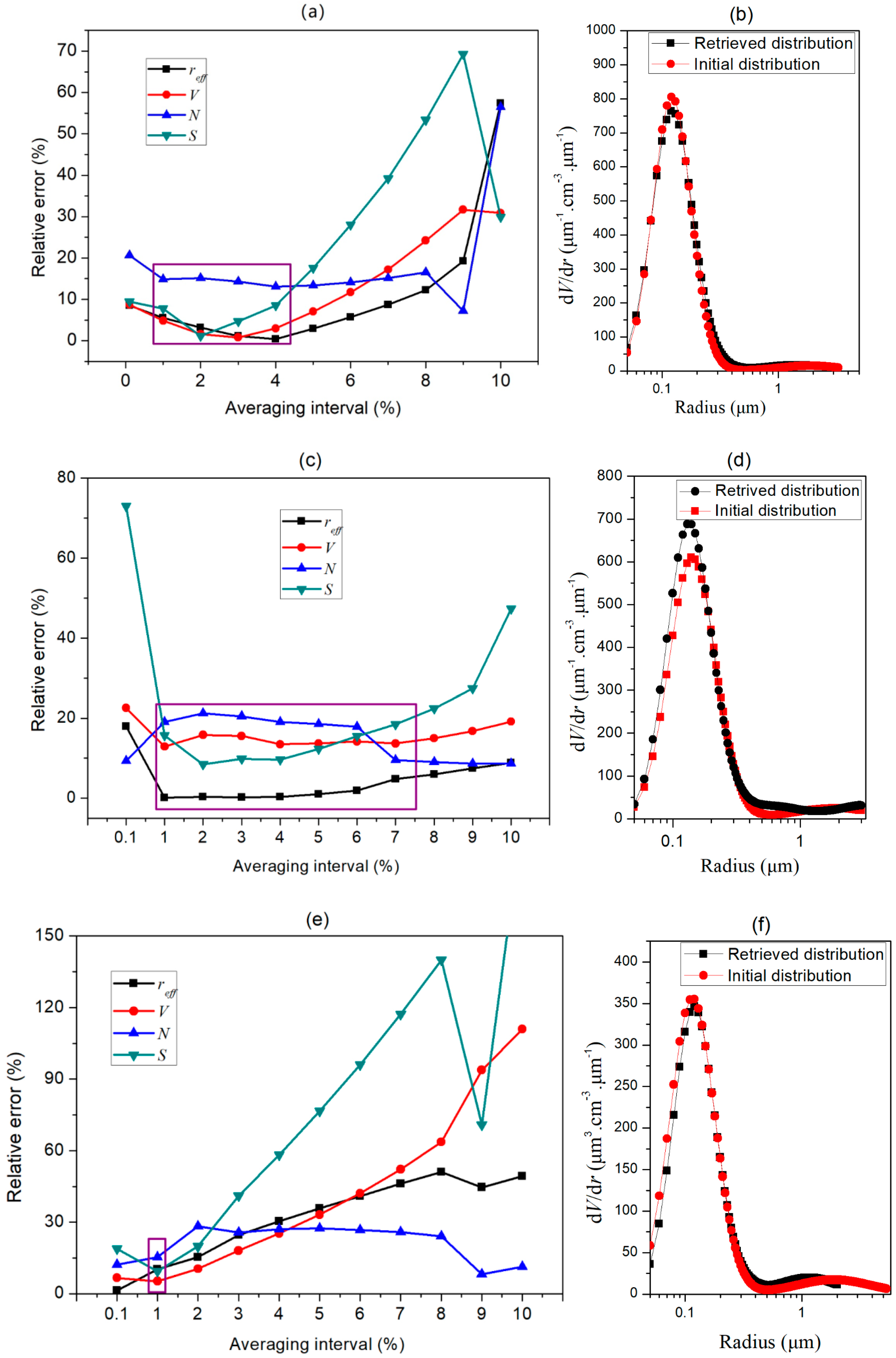
Three typical distributions were established according to the aerosol parameters in Table 1. The aerosols’ initial optical parameters were calculated from the distribution and complex refractive index. The authors’ algorithm was performed for the simulation. All possible complex refractive indices were chosen for the inversion. The real parts of the refractive index varied from 1.3 to 1.7 in steps of 0.01, and the imaginary parts varied from 0 to 0.03 in steps of 0.001. The averaging calculation was performed to stabilize the procedure. The averaging solutions for the aerosol microphysical parameters near the minimum of the discrepancy ρmin and the corresponding inversion of distribution are illustrated in Figure 2. The effective radius (reff), volume concentration (V), number concentration (N), and surface concentration (S) as functions of the averaging interval ρave are shown in the figure.
From Figure 2a,c,e, the best averaging interval of ρave is not a fixed value, and it changes with aerosol types and distributions. When the averaging interval ρave is between 1% and 4% for an urban industrial distribution, the inversion error of the microphysical parameters is less than 20%. If ρ > 5% and ρ < 7%, the values of reff, V, and N change slowly, and can be less than 20%. For S, there is a fast rise in relative error for ρave > 5%. Therefore, the authors chose 1–4% as the averaging interval for distribution 1. When the averaging interval ρave is 1–7% for biomass burning aerosols (distribution 2) (Figure 2d), the lowest inversion error of the microphysical parameters is found. The largest error can be found when ρave is 0.1%. For desert dust/oceanic aerosols, the best averaging interval ρave is 0–1%. The error of N varies slowly when ρave is between 0.1–8% according to Figure 2a,c,e. The error of S changes the fastest when the value of ρave is 0.1–9%. The most accurate results can only be achieved when ρave is 1%. The error of reff and V is less than N and S, and their change with ρave is related to the aerosol type. An average of approximately 1% of the total number of solutions arrived at the best estimate of the aerosol micro-parameters. The authors chose 1% as their final averaging interval. Figure 2b,d,f shows the retrieval of aerosol size distribution (black square–solid line) for (a) urban industrial aerosol distribution, (c) biomass burning aerosol, and (e) desert dust/oceanic aerosol, and their initial bimodal aerosol size distributions (red dot–solid line). From these results, the authors’ algorithm can well reconstruct the size distribution of aerosol particles. Besides the three sets of aerosol parameters in Table 1, more sets of aerosol parameters were also performed using the averaging interval analysis. The 1% averaging interval was still the best result.
4. Method Testing
Following the classification of the referenced atmospheric aerosols, the authors generated several types of bimodal lognormal distributions to test their algorithm. Table 2 shows the typical variability of the aerosol parameters for these aerosol types based on measurements from the worldwide Aerosol Robotic Network (AERONET) [21]. According to the parameters in Table 2, 40 sets of aerosol size distribution parameters were randomly selected for simulation calculations. The authors supposed that the aerosols were all spherical particles, and their extinction and backscattering coefficients were calculated using the Mie scattering simulation. For the non-spherical particles, Veselovskii et al. has discussed and provided the according algorithm in [20]. These contents will not be discussed in this paper. The generated aerosol size distributions are shown in Figure 3. The black curves show the urban industrial aerosol, the purple line represents the biomass burning aerosol, and the grey line represents the desert dust/oceanic aerosol. Two complex refractive indices were selected for one type of aerosol. For the urban industrial aerosol, the indices are 1.43 − 0.005i and 1.47 − 0.01i; they are 1.48 − 0.015i and 1.51 − 0.019i for the biomass burning aerosol; and they are 1.37 − 0.002i and 1.55 − 0.003i for the desert dust/oceanic aerosol.
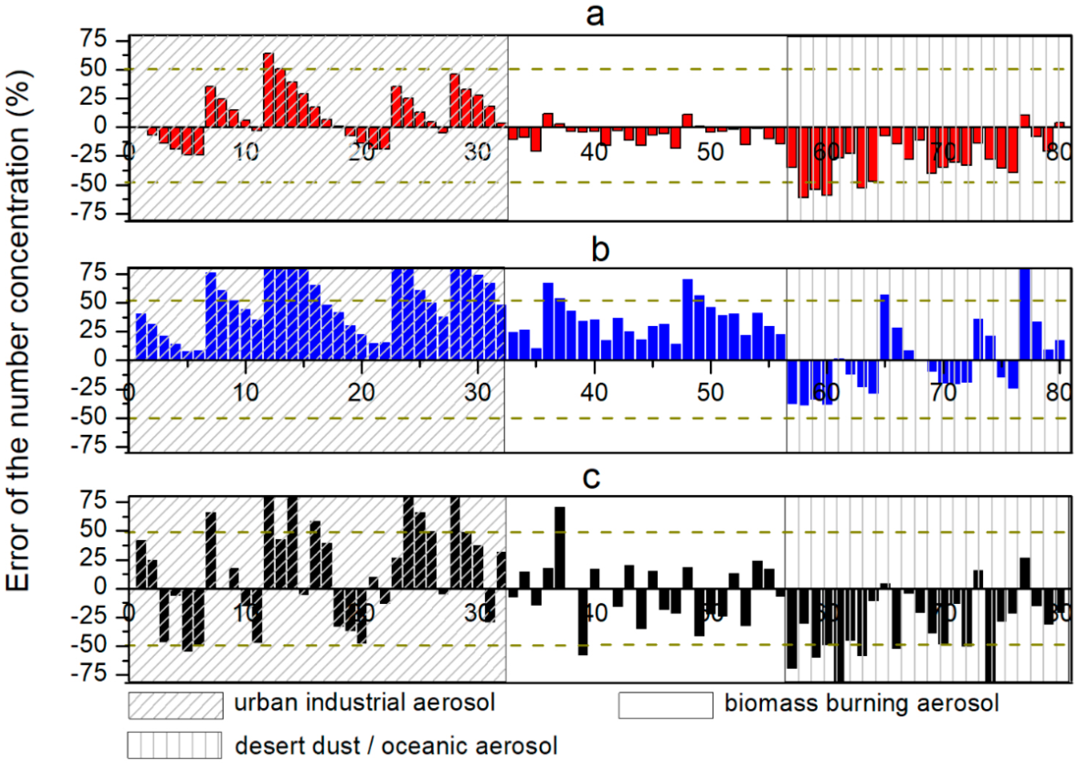
The 80 sets of idealized extinction and backscattering coefficients can be generated from the 40 aerosol distributions and two indices. The lidar system is complex and generally possesses random and systematic errors. Systematic errors in lidar systems come from many different sources, such as the nonlinearity of a photodetector, errors in the assumed atmospheric molecule density profile, or the use of an incorrect extinction-to-backscatter ratio. Random errors arise naturally from the measurement process. The systematic and random errors were considered in the tests of the authors’ algorithm. They assumed that there were systematic errors of an absolute magnitude of 10%. A +10% error was performed at α355 and β1064, and a −10% error was performed at α532, β532, and β355. Additionally, 15% random errors were also assumed in all the optical data. The two sets of data with errors as well as the idealized data were generated and used for the algorithm test. The authors performed the regularization retrieval with the three sets of data. The optimization algorithm described in the previous section was used to reconstruct the particle size distribution shown in Figure 3. Then, the corresponding microphysical parameters and errors were also calculated. The relative errors are shown in Figure 4, Figure 5 and Figure 6. Figure 4 displays the effective radius inversion error, Figure 4a is the error from the error-free data, Figure 4b is the error obtained from the 10% systematic error data and Figure 4c is the error based on the data with a 15% random error. Figure 5 shows the inversion error of the volume concentration from the three sets of data, and Figure 6 is the inversion error of the number concentration. The data in the medium-slant shadow area is the urban industrial aerosol, the blank area is the biomass burning aerosol, and the sparse vertical line shadow area represents the desert dust/oceanic aerosol.
Figure 4, Figure 5 and Figure 6 show that the systematic and random errors of the optical parameters increase the inversion error of the microphysical parameters. The effective radius has the smallest inversion error. Additionally, more than 95% of the effective radius errors can be controlled within 25% when the data are error-free. In the worst case, the effective radius was retrieved with an accuracy of 39%. More than 90% of the effective radius errors are less than 30% when the 10% systematic errors of all optical parameters are considered. More than 80% of data have errors of less than 30% if there are 15% random errors. Notably, ~4% of the data error is more than 60% when there are random errors of 15%. When systematic and random errors were considered, more than 95% data error was less than 40%. More than 90% of the volume concentration errors can be controlled within 45%, and the maximum error can reach 55% for the idealized extinction and backscattering coefficients. In the cases of large errors for the volume concentration inversion, the aerosol type is mainly biomass burning aerosol. Approximately 80% error of the volume concentration can be controlled within 50% even if 10% systematic error and 15% random error are performed on the optical parameters. The inversion accuracy is the worst for number concentration. In that case, 90% of the number concentration errors can be controlled within 50% when the data are error-free, and more than 80% of the resulting errors are less than 40%. When there are errors considered, 80% of the number concentration error can be controlled within 50%.
In analyzing the influences of different aerosol types on the inversion results, the authors observed that the effective radius error and the volume concentration for urban industrial aerosols was relatively small, whereas the number concentration error was relatively large. When the data were error-free, the maximum effective radius error was less than 39%, and the inversion error of volume concentration was less than 52%; however, in the worst case, the number concentration error could reach 60%. The effective radius and number concentration of biomass burning aerosols had an accuracy of 23%, and the volume concentration had an accuracy of 55%. The comprehensive errors for desert dust/oceanic aerosols were relatively large. The complex refractive index also influenced the inversion. Even with the same ASD, the inversion error changed when the aerosol complex refractive index changed. The errors of optical parameters increased the instability of the inversion, but because of the averaging method, most inversion results were still within a certain range.
The authors’ analysis was performed by combining the results with the distributions in Figure 3. The first peak of the biomass burning aerosol involved in the simulation was smaller and the second peak was larger than that of the urban industrial aerosol. The optical parameters input in the authors’ algorithm were 3α + 2β at 355 nm, 532 nm, and 1064 nm. There was a weaker inversion ability for the particles smaller than 0.1 μm and larger than 3 μm, so the inversion error for microphysical parameters for the biomass burning type was larger than the urban industrial type. The first peak of desert dust/oceanic aerosol was smaller than that of the urban industrial type. The second peak, though smaller, accounted for a larger proportion of this type, so the inversion error was larger overall. If the inversion accuracy of the biomass burning aerosol and desert dust/oceanic aerosol is to be improved, it will be necessary to select a shorter wavelength and a longer wavelength laser on the detection wavelength to increase the detection ability of smaller and larger particles.
5. Inversion of Actual Aerosol Size Distribution
The aerosol size distributions are complex and changeable under actual atmospheric conditions. They are not limited to a bimodal lognormal distribution but may be tri-modal or fourth-modal. To further verify the optimized algorithm, the aerosol distributions detected by the particle size spectrometer were calculated, analyzed, and retrieved. Aerosol measurements were collected over the surrounding areas of Beijing, Northern China from 2005 to 2007 using the airborne Particle Measuring Systems (PCASP-100X, PMI Co. Ltd., Longmont, CO, USA) of the Weather Modification Office of Hebei Province. The PCASP-100X is an optical particle counter for measuring aerosol size distributions from 0.10 μm to 3.00 μm in diameter in 15 different sized bins.
Aerosol profile data at a height of 0–4 km were selected for research and analysis. A set of particle distributions at every ~0.5 km was retrieved. The complex refractive index was unknown for the measured aerosol; the complex refractive index was selected as the urban industrial aerosol and the complex refractive index was chosen as 1.49 − 0.003i when calculating the extinction and backscattering coefficients from the distributions. Systematic and random errors were considered for the test. Figure 7 shows the measured aerosol size distributions at heights of 379 m and 605 m and the retrieved distributions using the authors’ algorithm.
The red dot in Figure 7 shows that the aerosol concentration measured fluctuates greatly in practice. The calculated particle size distribution basically reconstructed the characteristics of the bimodal distribution of the actual particle size spectrum. When errors were considered in the inversion, the retrieved distribution concentrations of fine mode and coarse mode fluctuated with error, and there were the opposite changes for the concentrations of fine mode and coarse mode when the errors were considered. The geometric mean radius and the mode width had little change.
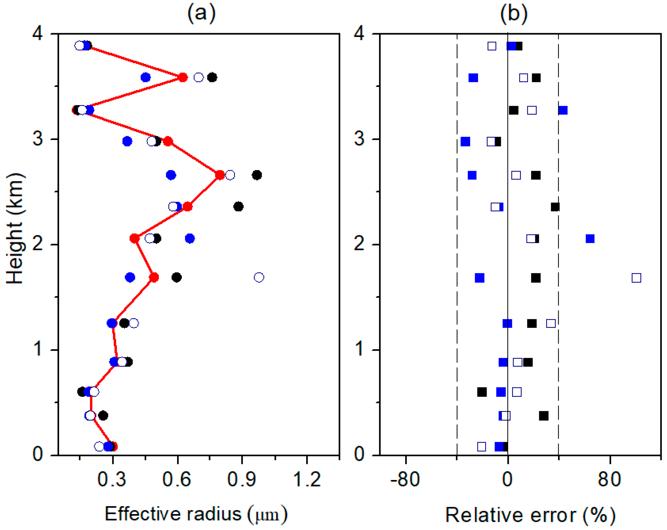
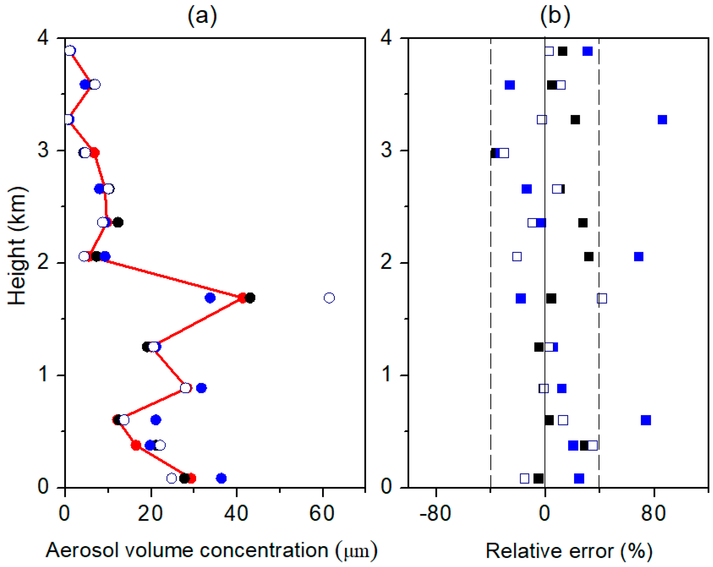
Based on the practical distributions and inversion results, the initial microphysical parameters and retrieval values were calculated, as illustrated in Figure 8, Figure 9 and Figure 10. The microphysical parameters were calculated and retrieved in three cases. The left figures illustrate measured values and retrieved values of microphysical parameters, and the right figures show their relative error in vertical height. Red dot–solid lines in the left figures are the microphysical parameters (effective radius, volume concentration, and number concentration) calculated from the measured data. Dark-solid dots in the left figures are the retrieved results from the error-free input data, and dark-solid squares in the right figures are the corresponding relative errors. Blue-solid dots and blue-solid squares are, respectively, the retrieved parameters and errors from the data with 10% systematic error. Navy hollow circles and hollow squares are, respectively, the results and error from the data with 15% random error.
The authors observed that the inversion of the microphysical parameters could be performed using their methods. When data was error-free, the maximum relative error of the effective radius was 35%, and the error for more than 80% of the inversion results was less than 25%. When the errors of optical parameters were considered, the inversion accuracy of effective radius was reduced. The worst relative error could reach 95%. Fortunately, this rarely happens. More than 95% of the effective radius errors can be controlled within 40%. The maximum error of the volume concentration was 29% for error-free input data, and the values of more than 80% of the data were less than 20%. When there were 10% systematic errors and 15% random errors for five optical parameters, 85% of errors were less than 40% and the worst error could reach 80%. The inversion error of the number concentration was less than 30% for error-free data. Systematic and random errors greatly affect the accuracy of inversion of number concentration. The worst relative error can reach 80%. The inversion error of the effective radius and volume concentration was small, whereas the inversion error of the number concentration was relatively large. As a whole, there were fewer retrieval errors for the actual data than the simulated data in Section 4. This is because the diameter of the measured ASD is in the range of 0.1 μm to 3.00 μm, whereas the diameter of the simulated ASD is in the range of 0.01 μm to 20 μm.
6. Discussion and Conclusions
Based on Tikhonov’s inversion with regularization, the inversion algorithm of aerosol size volume concentration was optimized by choosing the base function closer to aerosol distribution and a modification of the discrepancy principle. In this study, a logarithmic normal distribution function instead of the triangle function was selected as the base function for the inversion. The averaging procedure stabilizing the inversion was carried out for three main types of aerosols. The 1% averaging result near the minimum of the discrepancy showed the best estimate of the particle parameters. The stability and accuracy of inversion could be further stabilized.
Based on the previous aerosol distribution parameters, scores of aerosol size distributions were randomly generated for the authors’ algorithm test. In the worst case, the effective radius, volume, and number concentrations were retrieved with accuracies of 39%, 55%, and 60%, respectively, for the idealized data. More than 95% of the effective radius errors could be controlled within 25%, and more than 90% of the volume and number concentration errors could be controlled within 45% and 50%. When 10% systematic error or 15% random error were considered into the input optical parameters, there was an increase error in the inversion. More than 95% error of effective radius can be less than 40%, approximately 80% error of the volume concentration can be controlled within 50%, and 80% of the number concentration error can be controlled within 50%. Vertical height aerosol distributions detected by an airborne particle size spectrometer were used to test the authors’ method. This study represents the first time that actual aerosol size distribution was tested using the algorithm. The errors for the effective radius, volume concentration, and number concentration were calculated at the different heights. More than 95% of the effective radius errors can be controlled within 40%, 85% of volume concentration errors are less than 40%, and 90% of number concentration errors are less than 60%.
Author Contributions
Conceptualization, H.D. and D.H. Methodology and writing, H.D. Resources, H.D., Q.W., and H.H. Original draft preparation, H.D. Writing, H.D. and D.H. Review and editing, S.L., Q.Y., and J.L. Visualization, Q.Y., J.L., and Y.S. Supervision, H.D. and D.H. Project administration H.D., Y.S., and D.H. Funding acquisition, H.D. and D.H.
Funding
This work was supported by the National Natural Science Foundation of China (NSFC) (Grant Nos. 61575160, 41627807 and 61875163).
Acknowledgments
The authors would like to thank Mao Jietai from Peking University and the Hebei Artificial Impact Weather Office for providing airborne aerosol measurement data and suggestions for this paper.
Conflicts of Interest
The authors declare no conflicts of interest.
References
- Kwon, H.L.; Young, J.K.; Min, J.K. Characteristics of aerosol observed during two severe haze events overKorea in June and October 2004. Atmos. Environ. 2006, 40, 5146–5155. [Google Scholar]
- Quan, J.; Tie, X.; Zhang, Q.; Liu, Q.; Li, X.; Gao, Y.; Zhao, D. Characteristics of heavy aerosol pollution during the 2012–2013 winter in Beijing, China. Atmos. Environ. 2014, 88, 83–89. [Google Scholar] [CrossRef]
- Wang, Y.; Zhuang, G.S.; Sun, Y.L. The variation of characteristics and formation mechanisms of aerosols in dust, haze, and clear days in Beijing. Atmos. Environ. 2006, 40, 6579–6591. [Google Scholar] [CrossRef]
- Iwona, S.S.; Mateusz, S.; Olga, Z.; Kamila, M.H.; Lucja, J.; Patryk, P.; Domonika, S.; Birgit, H.; Wang, D.X.; Karolina, B.; et al. Modification of Local Urban Aerosol Properties by Long-Range Transport of Biomass Burning Aerosol. Remote Sens. 2018, 10, 412. [Google Scholar]
- Di, H.G.; Hua, H.B.; Cui, Y.; Hua, D.X.; He, T.Y.; Wang, Y.F.; Yan, Q. Vertical distribution of optical and microphysical properties of smog aerosols measured by multi-wavelength polarization lidar in Xi’an, China. J. Quant. Spectrosc. Radiat. Transf. 2017, 188, 28–38. [Google Scholar] [CrossRef]
- Műller, D.; Wandinger, U.; Ansmann, A. Microphysical particle parameters from extinction and backscatter lidar data by inversion with regularization: Theory. Appl. Opt. 1999, 38, 2346–2357. [Google Scholar] [CrossRef] [PubMed]
- Behrendt, A.; Wagner, G.; Petrova, A.; Shiler, M.; Pal, S.; Schaberl, T.; Wulfmeyer, V. Modular lidar systemsfor high-resolution 4-dimensional measurementsof water vapor, temperature, and aerosols. Proc. SPIE 2005, 5653. [Google Scholar] [CrossRef]
- Whiteman, D.N. Examination of the traditional Raman lidar technique. I. Evaluating the temperature-dependent lidar equations. Appl. Opt. 2003, 42, 2571–2592. [Google Scholar] [CrossRef] [PubMed]
- Whiteman, D.N. Examination of the traditional Raman lidar technique. II. Evaluating the ratios for water vapor and aerosols. Appl. Opt. 2003, 42, 2593–2608. [Google Scholar] [CrossRef] [PubMed]
- Veselovskii, I.; Whiteman, D.N.; Korenskiy, M.; Suvorina, A.; Pérez-Ramírez, D. Use of rotational Raman measurements in multiwavelength aerosol lidar for evaluation of particle backscattering and extinction. Atmos. Meas. Tech. 2015, 8, 4111–4122. [Google Scholar] [CrossRef] [Green Version]
- Johnathan, W.H.; Chris, A.H.; Anthony, L.C.; David, B.H.; Richard, A.F.; Terry, L.M.; Wayne, W.; Luis, R.I.; Floyd, E.H. Airborne High Spectral Resolution Lidar for profiling aerosol optical properties. Appl. Opt. 2008, 47, 6734–6753. [Google Scholar]
- Jagodnicka, A.K.; Stacewicz, T.; Karasiński, G.; Posyniak, M.; Malinowski, S.P. Particle size distribution retrieval from multiwavelength lidar signals for droplet aerosol. Appl. Opt. 2009, 48, B8–B16. [Google Scholar] [CrossRef] [PubMed]
- Donovan, D.P.; Carswell, A.I. Principal component analysis applied to multiwavelength lidar aerosol backscatter and extinction measurements. Appl. Opt. 1997, 36, 9406–9424. [Google Scholar] [CrossRef] [PubMed]
- Veselovskii, I.; Dubovik, O.; Kolgotin, A.; Korenskiy, M.D.; Whiteman, D.N.; Allakhverdiev, K.; Huseynoglu, F. Linear estimation of particle bulk parameters from multi-wavelength lidar measurements. Atmos. Meas. Tech. 2012, 5, 1135–1145. [Google Scholar] [CrossRef] [Green Version]
- Veselovskii, I.; Kolgotin, A.; Griaznov, V.; Műller, D.; Wandinger, U.; Whiteman, D.N. Inversion with regularization for the retrieval of tropospheric aerosol parameters from multiwavelength lidar sounding. Appl. Opt. 2002, 41, 3685–3699. [Google Scholar] [CrossRef] [PubMed]
- Veselovskii, I.; Kolgotin, A.; Vadim, G.; Műller, D.; Franke, K.; Whiteman, D.N. Inversion of multiwavelength Raman lidar data forretrieval of bimodal aerosol size distribution. Appl. Opt. 2004, 43, 1180–1195. [Google Scholar] [CrossRef] [PubMed]
- Pérez-Ramírez, D.; Whiteman, D.N.; Veselovskii, I.; Kolgotin, A.; Korenskiy, M.; Alados-Arboledas, L. Effects of systematic and random errors on the retrieval of particle microphysical properties from multiwavelength lidar measurements using inversion with regularization. Atmos. Meas. Tech. 2013, 6, 3039–3054. [Google Scholar] [CrossRef] [Green Version]
- Di, H.G.; Zhao, J.; Zhao, X.; Zhang, Y.X.; Wang, Z.X.; Wang, X.W.; Wang, Y.F.; Zhao, H.; Hua, D.X. Parameterization of aerosol number concentration distributions from aircraft measurements in the lower troposphere over Northern China. J. Quant. Spectrosc. Radiat. Transf. 2018, 218, 46–53. [Google Scholar] [CrossRef]
- Shipley, S.T.; Tracy, D.H.; Eloranta, E.W.; Trauger, J.T.; Sroga, J.T.; Roesler, F.L.; Weinman, J.A. High spectral resolution lidar to measure optical scattering properties of atmospheric aerosols. 1: Theory and instrumentation. Appl. Opt. 1983, 22, 3716–3724. [Google Scholar] [CrossRef] [PubMed]
- Veselovskii, I.; Dubovik, O.; Kolgotin, A.; Lapyonok, T.; Girolamo, P.; Summary, D.; Whiteman, D.N.; Mishchenko, M.; Tanré, D. Application of randomly oriented spheroids for retrieval of dust particle parameters from multiwavelength lidar measurements. J. Geophys. Res. 2010, 115, D21203. [Google Scholar] [CrossRef]
- Dubovik, O.; Holben, B.; Eck, T.F.; Smirnov, A.; Kaufman, Y.J.; King, M.D.; Tanre, D.; Slutsker, I. Variability of absorption and optical properties of key aerosol types observed in worldwide locations. J. Atmos. Sci. 2002, 59, 590–608. [Google Scholar] [CrossRef]
Figure 1.
Base functions curve under a logarithmic scale. rg,1 of the first function (black line) is 0.14 μm, rg,2 of the second function (red line) is 0.31 μm, rg,3 of the third function (blue line) is 0.69 μm, rg,4 of the fourth function (dark cyan line) is 1.57 μm, and rg,5 of the last function (magenta line) is 3.54 μm.

Figure 2.
Estimation errors for number (N), surface (S), volume (V) concentration, particle effective radius reff, and averaged discrepancy as a function of the averaging interval for three main types of aerosols (a,c,e). Additionally, the retrieved volume size distribution (black square–solid line) for (b) urban industrial aerosol distribution, (d) biomass burning aerosol, and (f) desert dust/oceanic aerosol and their initial bimodal aerosol size distributions (red dot–solid line) are shown. The purple squares represent the chosen averaging interval of ρave.

Figure 3.
Particle volume size distribution involved in the simulation.

Figure 4.
Inversion error of the effective radius. (a) error of the effective radius from the error-free data (red columns); (b) error of the effective radius from the data with 10% systematic error (blue columns); (c) error of the effective radius from the data with 15% random error (black columns).

Figure 5.
Inversion error of the volume concentration. (a) error of the volume concentration from the error-free data (red columns); (b) error of the volume concentration from the data with 10% systematic error (blue columns); (c) error of the volume concentration from the data with 15% random error (black columns).

Figure 6.
Inversion error of the number concentration. (a) error of the number concentration from the error-free data (red columns); (b) error of the number concentration from the data with 10% systematic error (blue columns); (c) error of the number concentration from the data with 15% random error (black columns).

Figure 7.
Comparison of the aerosol distribution and inversion distribution detected at two heights of (a) 376 m and (b) 605 m. The red dot is the aerosol volume concentration distribution measured by PCASP-100X, distribution 1 (dark line) is the retrieved data from the error-free data, distribution 2 (blue dot–solid line) is the retrieved data from the data with 10% systematic error and the distribution 3 (navy circle–hollow line) is the result from the data with 15% random error.

Figure 8.
(a) Measured aerosol effective radius, inversion effective radii and (b) the corresponding relative errors at the vertical heights.
Figure 8.
(a) Measured aerosol effective radius, inversion effective radii and (b) the corresponding relative errors at the vertical heights.

Figure 9.
(a) Measured aerosol volume concentration, inversion volume concentration and (b) the corresponding relative error at the vertical heights.
Figure 9.
(a) Measured aerosol volume concentration, inversion volume concentration and (b) the corresponding relative error at the vertical heights.

Figure 10.
(a) Measured aerosol number concentration, inversion number concentration and (b) the corresponding relative error at the vertical heights.
Figure 10.
(a) Measured aerosol number concentration, inversion number concentration and (b) the corresponding relative error at the vertical heights.


Table 1.
Simulated parameters of bimodal lognormal aerosols.
| Aerosol Type | lnσf | lnσc | V1 | V2 | m | ||
|---|---|---|---|---|---|---|---|
| Urban Industrial | 0.14 | 2.7 | 0.38 | 0.6 | 100 | 50 | 1.41 − 0.003i |
| Biomass Burning | 0.17 | 3.0 | 0.42 | 0.7 | 100 | 100 | 1.48 − 0.015i |
| Desert Dust and Oceanic | 0.14 | 3.3 | 0.44 | 0.75 | 50 | 80 | 1.51 − 0.002i |
Table 2.
Typical parameters of different biomodal lognormal aerosol types a.
| Aerosol Parameter | Urban Industrial | Biomass Burning | Desert Dust and Oceanic |
|---|---|---|---|
| rg1 | 0.14–0.18 μm | 0.13–0.16 μm | 0.12–0.16 μm |
| lnσ1 | 0.38–0.46 | 0.4–0.47 | 0.4–0.53 |
| rg2 | 2.7–3.2 μm | 3.2–3.7 μm | 1.9–2.7 μm |
| lnσ2 | 0.6–0.8 | 0.7–0.8 | 0.6–0.7 |
| V1/V2 | 0.8–2.0 | 1.3–2.5 | 0.1–0.5 |
| Real part of index | 1.4–1.5 | 1.47–1.52 | 1.36–1.56 |
| Imaginary part of index | 0.003–0.015 | 0.01–0.02 | 0.0015–0.003 |
arg1 describes the volume radius for the fine mode of aerosol size distribution; rg2 is the volume radius in the coarse mode; lnσ1 and lnσ2 are the mode widths for the fine and coarse modes, respectively; V1/V2 is the ratio of volume in the fine and the coarse particle modes.
© 2018 by the authors. Licensee MDPI, Basel, Switzerland. This article is an open access article distributed under the terms and conditions of the Creative Commons Attribution (CC BY) license (http://creativecommons.org/licenses/by/4.0/).
Share and Cite
MDPI and ACS Style
Di, H.; Wang, Q.; Hua, H.; Li, S.; Yan, Q.; Liu, J.; Song, Y.; Hua, D. Aerosol Microphysical Particle Parameter Inversion and Error Analysis Based on Remote Sensing Data. Remote Sens. 2018, 10, 1753. https://doi.org/10.3390/rs10111753
AMA Style
Di H, Wang Q, Hua H, Li S, Yan Q, Liu J, Song Y, Hua D. Aerosol Microphysical Particle Parameter Inversion and Error Analysis Based on Remote Sensing Data. Remote Sensing. 2018; 10(11):1753. https://doi.org/10.3390/rs10111753
Chicago/Turabian StyleDi, Huige, Qiyu Wang, Hangbo Hua, Siwen Li, Qing Yan, Jingjing Liu, Yuehui Song, and Dengxin Hua. 2018. "Aerosol Microphysical Particle Parameter Inversion and Error Analysis Based on Remote Sensing Data" Remote Sensing 10, no. 11: 1753. https://doi.org/10.3390/rs10111753
Note that from the first issue of 2016, this journal uses article numbers instead of page numbers. See further details here.