Semantic Interpretation of Mobile Laser Scanner Point Clouds in Indoor Scenes Using Trajectories


1
Department of Earth Observation Science, Faculty ITC, University of Twente, P.O. Box 217, 7514 AE Enschede, The Netherlands
2
Independent Researcher, 46397 Bocholt, Germany
*
Author to whom correspondence should be addressed.
Remote Sens. 2018, 10(11), 1754; https://doi.org/10.3390/rs10111754
Submission received: 28 September 2018
/
Revised: 31 October 2018
/
Accepted: 1 November 2018
/
Published: 7 November 2018
(This article belongs to the Special Issue Mobile Laser Scanning)
Abstract
:The data acquisition with Indoor Mobile Laser Scanners (IMLS) is quick, low-cost and accurate for indoor 3D modeling. Besides a point cloud, an IMLS also provides the trajectory of the mobile scanner. We analyze this trajectory jointly with the point cloud to support the labeling of noisy, highly reflected and cluttered points in indoor scenes. An adjacency-graph-based method is presented for detecting and labeling of permanent structures, such as walls, floors, ceilings, and stairs. Through occlusion reasoning and the use of the trajectory as a set of scanner positions, gaps are discriminated from real openings in the data. Furthermore, a voxel-based method is applied for labeling of navigable space and separating them from obstacles. The results show that 80% of the doors and 85% of the rooms are correctly detected, and most of the walls and openings are reconstructed. The experimental outcomes indicate that the trajectory of MLS systems plays an essential role in the understanding of indoor scenes.
1. Introduction
Due to recent improvements, mobile laser scanners (MLS) became an effective means of data collection in urban and indoor scenes. Indoor mobile laser scanners (IMLS) are capable of quick data collection at a lower cost than terrestrial laser scanners (TLS). Three types of common IMLS devices can be distinguished: Handheld devices (e.g., Zeb-Revo), push-cart systems (e.g., NavVis Trolley) and backpack sytems (e.g., Leica Pegasus). Thanks to the MLS mobility, these devices can achieve a more complete coverage of cluttered scenes in a shorter time.
In addition to generating point clouds, IMLS systems generate a trajectory of the sensor positions, which is a valuable source for the scene understanding. The trajectory can be linked to the point clouds through the time stamp. In robotics, some researchers have exploited the robot’s trajectory to classify indoor places from both the trajectory and point clouds [1,2]. However, the trajectory can be more useful in understanding indoor scenes. In our research, the trajectory is used for the detection of openings, separating building floors and the detection of stairs. For example, the trajectory as a set of scanner positions is used for occlusion reasoning to discriminate between openings and occlusions. Furthermore, wall planes that are intersected by the trajectory can be used to detect doors. Points that belong to stairs can be extracted by using the trajectory of the stairs. Obviously, detecting stairs by trajectory analysis is only applicable for laser scanners that are operable on stairs, i.e., for backpack and handheld systems.
In addition to using the trajectories, our research introduces a method for detecting the permanent structure, such as walls, floors, ceilings, and stairs from point clouds. Most current indoor reconstruction methods are limited by assuming vertical walls and a Manhattan World [3,4,5] to reduce the complexity of 3D space. Few works deal with arbitrary wall layouts [6,7,8], but they are restricted to vertical walls and horizontal ceilings. Our method detects slanted walls and sloped ceilings exploiting the adjacency of permanent structures, based on the assumption that there is less clutter near the ceiling in indoor environments. Additionally, the arbitrary arrangements of walls (non-Manhattan-World) will be handled in this work. Our pipeline for semantic labeling of permanent structure uses detection of planar primitives labelled as wall, floor and ceiling, and their topological relations.
Room segmentation is another research problem in large-scale indoor modeling. In the literature, different approaches, such as Voronoi graphs, cell decomposition, binary space partitioning and morphology operators [9] are suggested for 2D and 3D room segmentation. Some of these methods have limitations, such as Manhattan-World constraints and vertical walls. Most of the room segmentation methods rely on the viewpoint [8,10] and require scanning with a TLS in each room [7]. However, as opposed to one scanning location per room, mobile laser scanning systems produce a continuous trajectory and assigning points per room based on the scan location is not possible. Similar to our method for trajectory analysis, refs. [11,12] exploit the trajectory for space subdivision. Although their focus is only on space subdivision and simple structure, their results support our motivation of using the trajectory for interpretation of point clouds.
In our pipeline, a novel method is suggested for partitioning interior spaces based on voxels and exploiting unoccupied space. Besides knowing the room layout, information about the doors, walkable space and stairs supports navigation planning. Therefore, voxels are used to identify the walkable space and the trajectory to identify the stairs and doors.
Reflective surfaces, such as glass, complicate the analysis of indoor point clouds. Such surfaces cause the appearance of “ghost walls” in the data that do not exist in the real building. Ghost walls may incorrectly be detected as part of the room layout and sometimes result in an incorrect room segmentation. The problem of transparent and specular surfaces is addressed in robotics applications [13,14]. We tackle this problem by comparing the time stamps of points with the time stamp of the nearest trajectory parts before starting the wall detection process. Using our method, some of the noise caused by the reflective surfaces can be corrected.
The contribution of this work is introducing methods for using the sensor trajectory as a valuable source for semantic labeling of IMLS points clouds. The result is not a watertight model, although it extracts a coarse 3D model from heavily cluttered data with the presence of noise. Some of the methods presented in this work (e.g., door detection) are limited to mobile laser scanner data because of use of the trajectory. Most of our methods are applicable to TLS point clouds as well. For example methods for the wall, floor, and ceiling detection can be implemented on both RGBD data and TLS point clouds. The proposed methods are tested on three types of mobile laser scanner data: Backpack systems, trolley systems (push-cart), and handheld devices. The rest of the paper explains the related work, and data collection, followed by the methodology for permanent structure detection, space partitioning and door detection in Section 4, Section 5 and Section 6, respectively. The results, evaluation and conclusion are described in Section 7 and Section 8.
2. Related Work
In this work, several known problems are addressed in the domain of indoor modeling, such as detection of permanent structures, room segmentation, opening detection and dealing with noise and reflective surfaces. For each of the cases, the state of the art is reviewed in the following subsections.
Data acquisition: The first step in any indoor modeling pipeline from real data is collecting data and preprocessing to clean up the data. The main sources of the data for indoor modeling in large scale are point clouds from LiDAR Systems or RGBD Systems. LiDAR systems could be TLS devices, such as RIEGEL VZ [15], FARO FOCUS [16], or MLS devices, such as the Google Cartographer backpack [17], Leica Pegasus backpack [18], NavVis M3 Trolley [19], VIAMETRIS iMS3D [20] and Zeb-Revo and Zeb-1 [21]. RGBD cameras, such as Matterport [22] and Google Tango [23], are another source of data for indoor modeling. However, RGBD cameras have less accuracy in comparison with TLS or MLS. Lehtola et al. [24] present a thorough review of various indoor mobile laser scanners based on Simultaneous Localization And Mapping (SLAM). According to their study, TLS systems have the highest accuracy, but less flexibility, than MLS for indoor data acquisition. Backpack and handheld systems have the most mobility, but at the cost of a lower accuracy than trolley and TLS devices. The trolley devices are constrained to near-flat surfaces; they cannot be used on staircases and steep slopes. RGBD cameras are accurate enough for indoor 3D modeling purposes and scene understanding, but not surveying goals. In our research, we only use the point clouds from laser scanner systems, such as the data from NavVis M3 Trolley, handheld Zeb-1, Zeb-Revo and a prototype backpack system (ITC Backpack) based on the proof of concept of 6DOF SLAM [25].
Reflective Surfaces: The first step after data acquisition is dealing with noise and artefacts. Often these artefacts come from transparent and specular surfaces. Koch et al. [14] investigate this problem to identify specular and transparent surfaces during scanning with a SLAM robot. Their goal is to identify and purge the corrupted points from the data on the fly or by post-processing. The intensity of the reflected laser pulse and the material of the surface (e.g., aluminum surfaces, glass, and mirror) often have unique distribution for discrimination of the transparent and reflective surfaces. However, the detection of transparent surfaces is more challenging because of the characteristic of the material. In another study by Foster et al. [13] the authors employ both the geometry and the angle of incidence between the laser and the surface during scanning. They suggest that in a particular angle of incidence, specular and glass surfaces are visible to LiDAR and glass can be detected.
Approaches to indoor reconstruction either from LiDAR point clouds or RGBD images can be categorized to three following categories:
Indoor Volumetric Reconstruction: These approaches involve volumetric primitive detection (e.g., cuboid) and are often computationally more expensive than grammar-based and Binary Space Partitioning (BSP) methods. However, volumetric methods have a better representation of non-Manhattan-World structures, slanted and rounded walls and sloped ceilings. Xiao et al. [26] employ inverse constructive solid geometry (Inverse CSG) to build the 3D model. A 3D CSG is generated by iteratively stacking 2D CSG models. Each 2D CSG model is produced with many line segments that form various rectangle primitives. Their approach cannot model rounded walls because their hypothesis is based on extracting rectangles. Mura et al. [10] apply the piecewise-planar detection and encode the adjacency of planar segments into a graph that represents the scene.
Indoor grammar-based Reconstruction: One popular modeling approach, especially in regular environments, is adopting a (shape) grammar [27,28,29], Lindenmayer Systems (L-systems) [30] or (inverse) procedural modeling [31,32,33,34] approaches for interiors. Becker et al. [5] use a combination of split grammar and L-system to reconstruct a 3D model for as-built BIM (Building Information Model). Their approach has a different view of the indoor space, since it divides the building into two main partitions as corridors and rooms. In another innovative approach, Ikehata et al. [3] introduce an indoor structure grammar consisting of eight rules. Their approach is limited to Manhattan-World structures and 2.5D space. In [29,35,36] authors apply simple examples of shape grammar to reconstruct indoor models that are clutter free.
Binary Space Partitioning (BSP) or cell decomposition: In the domain of indoor reconstruction, many researchers use BSP to tackle the problem of room segmentation. In indoor space partitioning, BSP is a piecewise-planar approach that subdivides the space in 2D cells and as an output generates a 2.5D model [4,7,37,38]. In using BSP, 2D approaches have the assumption of both vertical walls and horizontal ceilings, which is a shortcoming of the 2D-BSP. If BSP is implemented in 3D, it results in a 3D reconstructed model [10,39,40], where the limitations of vertical walls and horizontal ceilings can be lifted. Additionally, BSP methods are able to assign the 2D or 3D cells of space partitions to the rooms based on the viewpoint and ray-casting. However, it requires scan positions per room with enough overlap to make the room labeling process possible. The main problems of BSP approaches are the restriction of viewpoints, the emergence of ghost primitives and the computation cost for labeling the cells as inside and outside.
Opening Detection: Among the work for the indoor reconstruction of points clouds, some of them [3,7,41,42,43,44,45,46] consider the problem of opening detection (doors and windows) and in their final model reconstruct the openings. Doors are essential elements for route planning and space subdivision. In our definition openings are not just limited to doors, but any opening in the wall that could be passed by individuals and connect two spaces. However, in cluttered environments and because of the presence of the furniture and obstacles, many walls could have data gaps that can be falsely considered as openings. Adan and Huber [41] propose an occlusion test to detect windows in the walls. Ikehata et al. [3] use a grammar rule to add a door in the wall between two separate rooms such that the walls are connected through a doorway. Therefore, in their pipeline, the addition of the doors is after reconstruction of the room. In a recent work Diaz-Vilarino et al. [44] use the trajectory for door detection followed by an energy minimization to separate rooms with the known location of the doors. However, their example is a simple and clutter-free dataset. Another approach for door detection especially in the robotic domain is using images besides point clouds for detection of semi-open doors and closed doors. Quintana et al. [45] and Diaz-Vilarino [46] present such techniques for detecting closed doors from images and point clouds.
Similar to our approach, authors of [11,47] use the trajectory for semantic enrichment of indoor spaces. The authors exploit the fact that doors are the connecting elements of two spaces. By detecting the doors using the trajectory, it is possible to partition the trajectory and the space. This approach is only suitable for interiors with low level of transparent surfaces. Similarly, Zheng et al. [12] analyze the scanlines to find local geometric regularities and to detect openings. By using extracted information, such as doors from scan lines, it is possible to segment the trajectory to associated spaces and subdivide the space. Both approaches may have poor results in environment with a large number of transparent surfaces or when the operator of the laser scanner has inconsistent behavior.
There is a large body of literature regarding scene understanding in small-scale indoor spaces, such as the detection of objects in a kitchen [48,49] for robot operation or in a bedroom [50,51]. In large-scale there are works by Armeni et al. [52] for scene parsing, Mattausch et al. [53] using a similarity matrix in cluttered environment and Qi et al. [54] using deep learning for object classification. Some other works in the domain of indoor 3D reconstruction from point clouds use semi-automatic approaches to generate BIM models [55,56,57] or stochastic methods to make a hypothesis on generating floor plans [58].
Our work is innovative in terms of dealing with glass reflection problems using mobile laser scanners and exploiting the potential of trajectories as a supplementary data produced by MLS systems. This work can be further improved to reconstruct a complete 3D indoor model from complex structures. Furthermore, the generated navigable space can be used for route planning in 2D (e.g., pedestrians, wheelchair and robots) and 3D space (drones).
3. Data Collection and Preprocessing
The data for this research is captured with three different mobile laser scanner systems. Each system has advantages and disadvantages in terms of mobility and accuracy. The data is collected by means of NavVis Trolley [19], Zeb-1 [59], ZebRevo, and ITC Backpack, a backpack system that is developed in our department and is in the stage of proof of concepts [25], see Figure 1. All three systems use Hokuyo UTM-30LX as the laser rangefinder sensor.
According to the Hokuyo UTM 30LX specification [60], the accuracy of the sensor in indoor environments for the range between 0.1 to 10 m is ±30 mm, and in the range of 10 to 30 m is ±50 mm. Backpack and handheld systems have more mobility than push-cart systems (trolley) and are able to scan stairs, while push-cart systems deliver a better quality of point clouds in comparison to handheld systems [24].
In Section 3.1, the data and the trajectory from various MLS devices used in this research are presented. In Section 3.2 and 3.3, the process of identifying corrupted points caused by reflective surfaces and then the segmentation process are explained.
3.1. Point Clouds and the Trajectory
One advantage of MLS systems over TLS devices is that in addition to the point clouds, they provide the laser scanner trajectory. The trajectory is a dataset containing a discrete suite of the device’s location during data acquisition and is synchronized with the point cloud. Therefore, by means of time stamps stored in the trajectory and point clouds, it is possible to know which points are collected from which location in the trajectory. In our experiment, a 0.01 second time resolution is used to group points from each scanner position. Figure 2 shows the trajectories of various MLS devices. The z-value of the points in the trajectory varies depending on both the scanning system and the height of the operator for a backpack or a handled device. Because mobile devices are moving in the environment, there would be less occlusion, but more artefacts caused by glass surfaces. The next section explains how to deal with such corrupted points in the data.
3.2. Identifying the Artefacts from Reflective Surfaces
In addition to the noise introduced by SLAM, another source of the noise is reflective and transparent surfaces, such as glass and specular metals. The MLS devices that are used in our experiments do not use a multi-echo sensor similar to the one is used in Koch et al. [14]. In our process, the trajectory and ray casting are exploited to detect and remove these artefacts. According to Foster et al. [13], when a laser beam strikes a glass surface three cases will happen: (i) Most of the light (almost 92%) is transmitted through the glass; (ii) some light is reflected back under a specular angle; and (iii) a small percentage of the light is scattered. If part of the glass surface appears in the point cloud it is because the incidence angle of the beam is near the perpendicular angle to the surface. Therefore, in the presence of a lot of glass surfaces in environments, three types of objects would be present in the data:
- Objects behind the glass if the laser beam is transmitted. Since almost 92% of the light is transmitted through the glass, a lot of objects behind a glass surface are measured through the glass. However, these points are less reliable than a directly measured object.
- Objects in the front of a glass surface which are reflected in the glass. In this case, the glass is acting like a mirror or a specular surface. Therefore, in the point clouds a mirrored object will appear exactly at the same distance from the glass and with the same size as the real object. We call these virtual objects “ghost walls”. They are problematic because it could happen that the whole room is mirrored to the other side of the specular surface. This artefact occurs when the laser scanner is moving in a specific angle toward the glass surface, naturally the same angle that objects could be seen in the glass.
- Objects that represent the glass surface itself. If the laser beam is almost perpendicular or there is dust and other features on the glass, then part of the glass surface will be present in the point cloud.
Knowing above facts, it is possible to analyze the behavior of LiDAR systems in interaction with glass surfaces. Ghost walls could happen outside the building layout, where the façades are made of glass and the laser scanner is moving alongside a corridor. In this case, some of the indoor spaces are mirrored outside the building. Highly problematic ghost walls are those that occur inside the main structure. In such cases, detecting and removing them is challenging, but also important.
In our pipeline, ghost walls are detected and purged based on segments. Our method for semantic interpretation is a planar segmentation approach. Therefore, the point clouds are segmented with a surface growing algorithm [61]. To detect ghost walls, the time stamps of the points are compared with the time of the closest trajectory point. Logically, because ghost walls are mirrored, they often have a time stamp, which differs from the time stamps of their neighboring points (which were not mirrored), as well as from the time stamp of the nearest trajectory point. Each point in the data is labeled as reflected point for which the time Tpoint is more than Δt before or after the time Ttraj of the nearest trajectory location. Δt is the time lag between the points in a ghost wall surface and the closest trajectory time. Δt is obtained empirically, and is obtained by checking such artefacts in the data. After labeling the points, the segments of which the majority of the points are labeled as reflected, are selected as ghost walls. In the next step, these ghost segments are projected back to their correct location. This is a relatively simple process, because they are in the same distance of the glass surface that the real object is located. But first, the glass surface should be detected. The glass surface is located between the real wall and the ghost wall. To detect the glass surface, a ray is reconstructed from a point on the ghost wall to the corresponding trajectory (see the purple line in the Figure 3c). This ray intersects a segment which almost has an equal distance to the real wall and ghost wall. The intersected segment is the glass surface. After detecting the glass surface, the points on the ghost wall are mirrored back relative to the glass surface to the other side (white points in the Figure 3d). Finally, after correcting the data from the ghost walls, it is ready to be applied for further processing.
3.3. Segmentation and Generalization
Since most indoor environments are composed of planar structures, extracting and labeling of planar faces is faster and more reliable than processing individual points. Because of the clutter and noise in the data the result of a segmentation cannot directly be used for semantic labeling and reconstruction. To generate planar patches that represent permanent structures, such as walls, floors and ceilings, a generalization method will be applied to the segments. For this purpose, we build on a method described by Kada [62] for generalization of 3D building models. Our adopted generalization method aims at merging segments based on their co-planarity, angle between normal vectors and their distance. First, all the segments are sorted by their size in terms of the number of points. Starting with the largest segment three criteria are considered to merge a candidate segment into the current segment: (i) A generalization distance (=D) should be satisfied to accept or reject the candidate segment for merging; (ii) the parallelism of two segments by comparing their plane normal vectors; (iii) bounding boxes of two segments should be within a certain distance (=d). The proximity is checked alongside two segments planes. For example, two coplanar segments alongside a corridor should be within a threshold d. We refer to the result of generalization as “surface patches (S)” and for each surface patch a plane is fitted to its point cloud using a least squares method. The generalization method decreases the number of segments to be analyzed significantly. Additionally, small segments will not disturb the process of semantic interpretation. For detecting permanent structures, described in the next section, surface patches will be used instead of segments.
4. Permanent Structure Detection
For the detection of walls, floors and ceilings, the surface patches that are generated in the previous step are further processed. An adjacency graph is constructed from the patches and is further analyzed to induce the correct class of each patch (Section 4.2). For the detection of openings, an occlusion reasoning method is applied to discriminate between real openings and gaps that are caused by occlusion (Section 4.3). The occlusion test is also used to remove points that are outside the building layout and could be disturbing the reconstruction process. To start with detecting the permanent structure, the building levels are separated and then each level is processed separately (Section 4.1).
4.1. Separation of Building Levels and Stairs
The typical solution in the literature [10,37,63] for separating building levels in indoor point clouds is using a height histogram of points. A level in a building is a horizontal section that extends over the floor space. Using the histogram is straightforward and gives an initial separation of the building levels. However, it is not applicable to buildings where a building level is extended vertically in the space to other levels (see Figure 4a) or a building with sub-levels. To overcome this problem in complex architectures, first the trajectory is separated to several levels and staircases. If the trajectory belongs to a handheld or a backpack system, the separation should be done where the operator enters the stairs. Therefore, the flat trajectory can be split from a sloped trajectory on the staircase. If the trajectory belongs to a push-cart scanner, then the trajectory of the levels are already separated, because the device does not move up or down the stairs.
To separate the levels, the process starts with the segmentation of the trajectory to the horizontal and sloped segments. A surface growing segmentation is used and points on the same horizontal or sloped plane are segmented together. Figure 4b shows that the trajectory points in the upper level (blue segment) belong to the same level and points on the staircases are segmented together. However, this segmentation needs a modification to make sure staircases are separated correctly. For example, if in the same level of the trajectory, there are several segments with a height difference of fewer than two meters (see Figure 4c, the orange and purple segments in the first floor) they will be merged. This is done because trajectories belonging to different levels typically have a height difference more than the ceiling height (at least two meters). After separating the trajectory to meaningful building levels, for each segment in the trajectory, the associated points from the point clouds will be selected using the timestamp.
Near the staircases, the laser scanner measures points from other levels; to modify the level of these points to their correct level, the two dominant horizontal planes are detected as floor and ceiling of the current level and the label of the points is changed to the corresponding levels. Figure 4d shows the first and third level of the building. After separation of levels, each level will be processed individually for detection of walls, floors, and ceilings.
The point clouds of the stairs are extracted using the trajectory segments of stairs and the associated timestamp. Figure 4e shows four different stairs datasets colored based on four segments of the trajectory. Because a large portion of other levels may be seen from stairs, it is sometimes inevitable to have an overlap between point clouds of the stairs and the floors. For example, in Figure 4e part of the floors are also scanned from the stairs.
4.2. Wall Detection
The wall detection process includes detecting the permanent structures, such as walls, floors and ceilings. This process starts by making an adjacency graph (G) from surface patches (S). An adjacency graph is presented by G = (V, E) where nodes (V) are surface patches and edges (E) are connecting two adjacent nodes. Each node is associated with the point clouds of a surface patch S. When a label (l) is assigned to a surface patch, all the associated points obtain that label. The label shows the class of the surface, such as wall, floor, ceiling, door, and window.
Two nodes (V) are adjacent if their corresponding surface patches are within a specific distance from each other. This distance is set to dadj = 0.1 meter in all of our experiments. Note that the coplanar or parallel segments are already merged. Therefore, two adjacent surface patches could meet under any arbitrary angle, which means our method is not limited to Manhattan-World. To deal with slanted walls and non-horizontal ceilings an angle threshold (α) should be specified to separate the candidate walls and ceilings before proceeding with the analysis of the graph. Each node in the graph is labeled as almost-vertical or almost-horizontal based on a threshold α. By default, this threshold is set to α = 45 degrees to make a primary separation between candidate ceilings and walls. Considering this threshold, the node V in the graph G will be categorized to Vh and Vv for almost-horizontal and almost-vertical. By comparing a pair of surface patches out of nodes V(v1, v2), three principal labels will be assigned to each edge e ϵ E of adjacent nodes v1, v2:
- E obtains the label wall-wall iff v1 and v2 are both almost-vertical and adjacent.
- E obtains the label wall-ceiling iff v1 and v2 are almost-vertical and almost-horizontal respectively and the center of v2 is higher than the center of v1.
- E obtains the label wall-floor iff v1 and v2 are almost-vertical and almost-horizontal respectively and the center of v2 is lower than the center of v1.
After labeling the edges, each node in the graph will be analyzed based on the connected edges and the respective labels. Three main rules are applied to each node v ϵ V to decide for the label:
- Rule 1.
- V obtains the label wall iff the count of wall-ceiling edges is equal or more than one and V is almost-vertical. This means every wall should be at least once connected to the ceiling.
- Rule 2.
- V obtains the label ceiling iff the count of wall-ceiling edges is more than two and the count of wall-wall is equal to zero. This means an almost-horizontal surface with wall-ceiling edges should be connected more than two times to the walls to get the ceiling label.
- Rule 3.
- V obtains the label floor iff the count of wall-floor edges is more than two and the count of wall-wall is equal to zero. This means an almost-horizontal surface with wall-floor edges should be connected more than two times to the walls to get the floor label.
Note that in Rule1, the connection of the wall candidates to the floor is not checked because of possibly heavy occlusions near the floor.
During the processing of the rules, further considerations as soft rules need to be applied. For example, during applying second and third rule on the ceilings and floors, each almost-horizontal surface cannot be a floor or a ceiling candidate. This happens especially in the case of horizontal surfaces of shelves and tables. Therefore, the average z-value of a horizontal patch is compared with an estimation of the floor and ceiling height to decide if it is near the floor or ceiling. In this way, horizontal surfaces of objects, such as tables and boxes, could be discarded. However, some of the horizontal surfaces that are near the floor and ceiling disturb the correct semantic labeling. For example, the top of shelves and cabinets that are near the ceiling could be labeled as the ceiling (see Figure 5b). As a drawback, the attached vertical surfaces that are connected to them may be also mislabeled as walls. To avoid this problem, the overlap of projection of almost-horizontal surfaces in the xy-plane is checked before starting with the rules. If the 2D projection of two horizontal surfaces has overlap (considering a small buffer), the upper surface is preserved as a ceiling candidate and then the process with the rules will follow. Since, the topological relations of the surfaces are exploited in our method, it is not limited to regular manmade structures or Manhattan-World.
In the permanent structure detection method, a ceiling or floor will be distinguished from a wall by the angle threshold which is by default α = 45 degrees. By applying rules 1, 2, and 3, a slanted surface could be labeled to a wall or ceiling (floor) depending on its normal angle. In our method, a slanted surface is distinguished by this angle threshold defined by the user. Figure 6 shows two different cases when α is set to 40 and 50 degrees. However, there is a special case where the slanted surface is distinguished as a wall and is supported by another vertical wall that is connected to the floor (see Figure 6b). Such a case happens when a slanted wall and a vertical wall are not segmented in the same surface patch since they have different normal angles during the generalization. Therefore, an extra check is required to see if the almost-vertical surface that is not connected to the ceiling is a wall or not. This check could be done by means of support and adjacency relation between a slanted surface and a vertical surface. Let v1 and v2 represent the two almost-vertical surfaces and one of them is not connected to the ceiling, then the lower one (with a lower center) is called supporter (v1) and the upper one is called the supported (v2). Furthermore, the condition max-z(v1) < min-z(v2) including a buffer should be satisfied. Notice that checking the support relation is necessary, otherwise objects attached to the wall could be labeled as a slanted wall. Respecting this explanation, the corresponding edge (E) of two adjacent wall candidates (v1, v2) could obtain the following label: E obtains the label wall-slantedwall iff v1 and v2 are both almost-vertical and the intersection line is almost-horizontal and one surface is supporting the other one.
The following rule is applied to define the label of a node V: Rule 4. V obtains the label slantedwall iff the count of wall-slantedwall edges is more than zero and the count of wall-wall edges is more than zero and V is almost-vertical.
Since a real dataset with slanted walls from a MLS system was not available, our algorithm is tested on a part of the penthouse dataset from Mura et al. [10]. We assumed the slanted surfaces once as the non-horizontal ceiling (α = 40) and once as slanted walls (α = 50). Figure 6 demonstrates the results on a part of the penthouse building. This experiment shows the robustness of the algorithm in case of non-horizontal ceiling or slanted walls. In the next section, a method is presented for detecting the openings by using the trajectory and applying occlusion-test.
4.3. Opening Detection Using the MLS Trajectory
After detecting the walls, floor and ceilings, the point clouds are enriched with more semantics, such as openings (doors and windows). Reasonably, it is expected that doors and windows are located on the walls. Furthermore, openings are represented as holes or gaps in the data because where there is an open door or a window the laser rays go through the wall surface. The same gaps happen in the data, if part of the scene is not captured by the laser scanner, e.g., because of occlusion. Therefore, one problem of opening detection is to discriminate between data gaps and real openings in the data. We exploit the fact that a laser beam, crossing a wall surface with the opening, hits the objects behind the surface. Hence, from each location on the trajectory a ray is reconstructed to the measured laser point. Note that here the time attribute of the points plays an important role. Because from every point on the trajectory only the measured points at that specific time are evaluated for the ray casting. This process is named occlusion-test and is implemented as the following (see Figure 7): First, each surface patch Si with the wall label would be enveloped by a 3D voxel grid (grid size of 10 cm). Second, a ray is constructed from t1 on the trajectory to the corresponding point p1 in the point cloud. If the ray intersects a surface s1 ϵ Si, the intersection point of the ray and the surface corresponds to one of the voxels of the s1. The incident voxel obtains one of the four labels: Occupied, occluded, open or unknown. The incident voxel is occupied if the measured point p1 belongs to the s1, occluded if p1 is in front of the s1, opened if p1 is behind the s1 and is unknown otherwise. If the ray does not intersect the surface the labels remain unchanged.
After the occlusion-test process, the results need to be further inspected to identify false openings. False openings happen where a clutter is connected to the ceiling and is extended to the neighboring walls. Therefore, during the occlusion test it is considered as a surface with opening (Figure 8b). Such false openings are identified and removed if more than a percentage (e.g., 80%) of voxels in the wall surface are labeled as openings (Figure 8c). With this simple check most of the false openings and erroneous walls are removed.
Furthermore, it is possible to separate the openings into openings that intersect the floor (doors), and those that are above the floor (windows). However, the clear frame of the opening could not be inferred because of the noise and occlusion.
The occlusion-test provides additional information about the points behind the wall surface. During the occlusion-test, points that are behind each surface are flagged for further inspection. Each point p1 that is behind the surface s1 and is measured from t1 on the trajectory, can be a reflected point or a point that is sensed through a transparent surface. In Section 3.2, it was explained how to identify points that are caused by the reflection. Otherwise, the point is labeled as a point-behind-surface artefact and will be removed from the collection. Here, the assumption is that the objects behind an opening are scanned properly from the belonging space. A point behind a surface is less reliable because it is possibly measured through a glass surface. For example, in one of the datasets (Fire Brigade building, level 2) some of the rooms are partially mirrored to the outside of the building, because of a lot of glass surfaces in the façade. Consequently, in detecting the permanent structures they are mislabeled as walls, floors and ceilings. By removing points behind a surface, artefacts that are outside the building layout and could not be identified as reflection will be removed.
5. Space Partitioning
Space partitioning is the process of separating space into more meaningful partitions that could be differentiated by permanent structures. Every space represents a room or a corridor. Unlike other methods that use a 2D projection of walls into xy-plane and applies cell decomposition, our method relies on volumetric space partitioning (Section 5.1). Therefore, slanted walls and non-horizontal ceilings do not constrain our method. For this purpose, a voxel space with the voxel-size of 0.10 m is exploited. In Section 5.2, the navigable and non-navigable spaces are extracted from the voxels.
5.1. Volumetric Space Partitioning
A voxel space is generated from the point clouds for space partitioning. Voxels are labeled with the permanent structure semantics. The occupied, opening and occlusion labels (Section 4.3) are transferred to the voxels as occupied label. Rest of the voxels are labeled as empty (unoccupied). Including the label of openings and gaps is important for space partitioning, because spaces can be connected through openings (e.g., a window) or gaps (e.g., an occlusion). Therefore, the dataset that is used to label voxels contains openings, occluded areas, walls, floors and ceilings.
After labelling the voxel space to occupied and empty, three main steps generate the spaces: (i) A morphological erosion method is applied on the empty voxels. Therefore, the area covered by occupied voxels will grow and empty voxels with weak connections will be separated; (ii) A connected component analysis is applied on selected empty voxels from the previous step to make separate clusters of empty connected voxels. Each cluster at this stage represents a space partition; (iii) Then a morphological dilation is applied on empty voxels, while this time empty voxels have a cluster number. Consequently, the area covered by empty voxels grow while occupied voxels area is shrinking. Finally, each cluster of empty voxels represents a space partition.
This approach has two advantages, it is volumetric and it is independent of Manhattan-World constraints. However, the empty voxels that are present outside the building layout will generate some invalid spaces that need further attention. In the following, we explain how to modify these invalid spaces.
Validating Space Partitions Using the Trajectory: In case the building layout is known, for example from a ground plan, it is possible to detect and remove invalid spaces generated outside the building structure. However, our pipeline is just relying on the geometry of the point clouds. Therefore, by using the trajectory, spaces that are not traversed during the data collection will be discarded. In other words, space partitions (e.g., rooms, corridors) are representing empty spaces in the environment that have intersection with the trajectory. A kd-tree search algorithm is used to check a partition’s intersection with the trajectory. Furthermore, the space partitioning process is retained as a volumetric solution and projecting spaces to xy-plane is avoided (because of possible slanted walls). For each partition, the nearby trajectory is found and if the distance is less than the voxel size it indicates the intersection, hence, a valid partition. This can be done in 3D and it enables us to discard outside partitions that are not navigated by the trajectory. This approach is favored over methods of calculating the alpha shape of a partition in 3D or the minimum enveloping polygon in 2D to check the intersection with the trajectory, because an alpha shape or a minimum enveloping polygon cannot precisely represent the complex shape of a space partition. Figure 9 shows the spaces and the trajectory from different views.
During the space partitioning process, each space partition represents only the empty space if the furniture is included in the process. This fact is exploited to generate the 3D navigable space. However, including furniture can cause over-segmentation of the space because some of the furniture can divide the space in the same room. Next section elaborates on the details of navigable space.
5.2. Extracting the Navigable Space
Having discussed how to generate space partitions, in the following, it is explained how to extract the navigable and walkable area out of the empty space. Each space partition represents the empty space (after including the furniture space). The navigable space can be generated in different heights above the floor and below the ceiling, which is suitable for flying objects to navigate in the space. Again, it is important that the gaps on the walls caused by the occlusion or opening are labeled as occupied in the voxels to avoid misinterpretation as walkable space. Doorways that are considered as openings are labeled as navigable in the final navigable space. Empty voxels just above the floor are extracted as walkable space. In Figure 9c,e, the spaces are illustrated from the bottom to show the carvings of the occupied spaces in the empty spaces. If some of the openings connect the spaces and they are not recognized during the opening detection, as a drawback few partitions cannot be split and remain as one space (e.g., the orange space in Figure 9). The void between the space partitions is caused by furniture and permanent structure.
6. Door Detection Using the Trajectory
In this stage, doors that are intersected by the trajectory during the data acquisition can be detected. Note that in Section 4.3, some doors were already detected as openings by occlusion tests, while here it is possible to detect closed doors as well. For detecting the doors using the trajectory, the voxels and the trajectory are the input data of the process. Voxels are used for this step, because the algorithm tries to find the center of each door that is crossed by the trajectory (see Figure 10).
The door center is represented by an empty voxel in case of an open door and an occupied voxel in case of a closed door. Each voxel in the voxel space is checked whether it can be a center of a door candidate (a door center). A voxel is a door center candidate if: (i) Nearby the voxel there is a trajectory; (ii) Above the voxel occupied voxels exist that represent top part of a door frame; (iii) The neighborhood of the voxel should be empty for an open door. These three criteria enforce three main search radius parameters: (1) A search range to look for a nearby trajectory (rtraj < * voxel-size); (2) a search radius to look for voxels on top of the door frame relative to the floor (1.80 m < rtop < 2.10 m); and (3) a neighborhood search radius (rvoid < n * voxel-size) to make sure around the candidate voxel is empty, where the search radius is a factor of voxel size. The rvoid threshold should always be smaller than the door width to exclude the door frame in the search for empty neighborhood. Empirically, if the percentage of empty voxels around a door center within the search radius (rvoid) exceeds 70% of the total neighbor voxels, then the third criteria for an open door is fulfilled. Furthermore, to speed up the calculation process, only voxels are explored to be a door center that are located in the height between 0.8 to 1.10 m relative to the floor, as the door center is expected to be in this height.
Closed Doors: Closed doors appear in the point cloud as part of the wall (Figure 10, the middle door). When the trajectory crosses the door and the door is closed before or after the scanning, it appears in the data as if the trajectory went through the wall. To detect closed doors crossed by the trajectory, the same three criteria as open doors are applied, but with the difference that for the third rule the neighborhood of the voxel candidate as the door center should be occupied instead of empty. Notice that simply intersection of wall planes with the trajectory is not sufficient to detect closed doors. Because in cluttered rooms the trajectory goes between the congested furniture or false detected walls that can be identified as false doors. Therefore, checking the three criteria is also required for closed doors. The door detection algorithm, using the trajectory, can only be used for spotting the location of the door (also double doors), further inspection is required for identifying the door frame or the door leaf.
7. Results and Evaluation
Our approach is tested on four datasets collected with four different mobile laser scanners. The details of the datasets and the scanners are given in Table 1. The results of all datasets and the ground truth are shown in Figure 11. The results show that 80% of the doors and more than 85% of the rooms are correctly detected. Our methods are tested on buildings that violate the 2.5D and Manhattan World assumptions. The space partitioning results (Figure 11, 3rd column) show our constraint-free approach in arbitrary room layouts with different ceiling heights. Both datasets from Fire Brigade building level 1 and the TU Delft Architecture building have large halls with a high ceiling and different ceiling heights in other rooms. Figure 11 (3rd column, first and last row) illustrates the extracted spaces for these two datasets. The permanent structures in Figure 11 (2nd column) indicates that our pipeline is capable of detecting most of the walls and openings in the heavy cluttered environments with many reflective surfaces.
Each dataset is subsampled to ease the visualization and to decrease the processing time. For subsampling, every k’th point of a kNN is used, where a reduction factor between 4 and 6 is applied to decrease the size of the original dataset while keeping the structure of the point clouds. The subsampling keeps the average point distance less than 0.05 m.
The other important influential factors are noise, the level of clutter and the number of glass surfaces in the data. The level of noise depends on the sensors precision and the SLAM algorithm. For details of each MLS device accuracy and noise, the readers are referred to the specification of each product and the review by Lehtola et al. [24]. In terms of high clutter and high number of glass surfaces, Fire Brigade dataset poses a lot of challenge because of the very large glass walls. Such glass walls, as well as heavy clutter are present on the first floor (Figure 12), where the fire trucks are located.
Implementation: All algorithms are written in C++ and tested on a Lenovo ThinkPad workstation with an Intel core i7 (2.5 GHz), 16 GB RAM. The main computational cost is devoted to occlusion test process, because of the ray casting algorithm where the peak of RAM usage is 16 GB and for large datasets it takes up to an hour. Another expensive process is space partitioning, because of the 3D morphological process on a large number of voxels. For an area with almost 15 million voxels, it takes 10 minutes with a voxel size of 10 cm, and 3 minutes with a voxel size of 20 cm. Other algorithms including permanent structure detection, door detection, reflection removal, level partitioning and surface growing take seconds up to 5 minutes depending on the size of the dataset. The computation time for space partitioning is more dependent on the volume of the building and height of the ceiling than the size of the point clouds. For example, for the TU Delft dataset the number of voxels exceeds 100 million, since the orange hall has high ceilings (almost 13 meters). Therefore, the space partitioning method is implemented with 20 cm voxel size for this dataset to speed up the process.
Parameter Selection: Our pipeline starts with the surface growing segmentation followed by a surface patch generalization algorithm. For the surface growing segmentation the most important parameter is the smoothness threshold. The optimal value depends on the amount of sensor noise and the noise caused by the SLAM algorithm. For the MLS devices in this article, the sensor noise is less than 5 cm. However, there is more noise in the data created by SLAM algorithm and artefacts of the glass reflections. Therefore, we experienced a value between 10 and 15 cm for datasets from Zeb1 as a good threshold for planar segmentation and between 5 to 10 cm for other datasets (ZebRevo, ITC Backpack and NavVis Trolley). For the surface patch generalization, nearby surfaces are considered parallel if their normal vector angle tolerance is less than θ < 10°, and their proximity (d) alongside the plane is less than 60 cm. The time lag Δt is the important parameter for detecting and pruning of ghost walls. Empirically, we choose 150 seconds time lag for a point to be considered as a reflected point, and if more than 70% of the points in a segment have this time difference with their neighbor trajectory that segments is defined as a ghost wall.
For reconstructing the adjacency graph, the distance for adjacency of two surface patches is less than dadj < 10 cm and the minimum length of an intersection line is 20 cm. We experienced that a minimum length of 20 cm in most datasets is reasonable. There is just one special case that the threshold is increased to 25 cm, when the frames of doors are extended to the ceiling (e.g., glass rooms in Figure 13). To avoid door leaves to be misclassified as wall, a minimum length of 25 cm for intersection line is considered.
The default threshold of 45° is considered for separating the surfaces to almost-vertical and almost-horizontal. In case of different sloped ceilings, the angle threshold could be changed to recognize the ceilings from slanted walls. The minimum number of supporting points for each surface to be included in the adjacency graph is 500 points. A voxel size of 10 cm is preferred for algorithms operating on voxels, such as the occlusion test, space partitioning and door detection. For a point spacing of 2 to 5 cm, the voxel size of 10 cm offers a good balance between the computational time and the number of preserved details of permanent structures. The window size of the morphological operator for the space partitioning should be larger than a doorway to ensure the separation of spaces at the locations of open doors. Therefore, a window size between 1.0 to 1.3 m is suggested. Other soft parameters, such as kNN search, proximity search and connected components do not have significant influence on the whole pipeline.
Robustness: The robustness of our algorithms is evaluated by testing on various datasets collected by four different mobile laser scanning devices. Additionally, our pipeline is tested on a multistory building (Fire Brigade dataset), a building with slanted walls (Figure 6) and different ceiling heights (Fire Brigade building, level 1 and the TU Delft Architecture building), and a building with high amount of clutter and glass surfaces (Cadastre building and Fire Brigade building, level 2). Among those, buildings with large glass walls pose the largest challenge to our pipeline (for wall detection and space partitioning), because the connection of glass surfaces near the ceiling is not guaranteed in the segmented data and in some cases these glass surfaces are missing entirely in the data (the TU Delft Architecture building the hall with orange stairs, Figure 14). However, the wall detection is capable of detecting glass walls even with loose connections to the ceiling.
For reconstructing the adjacency graph, all datasets are processed with dadj 10 cm. We experienced, in most cases that increasing this threshold to 20 cm or higher results in losing some of the walls; and decreasing the threshold to less than 10 cm results in misclassification of some clutter surfaces to wall surface. The dadj parameter depends on the noise in the data. For datasets with a higher level of noise the threshold could be increased to 20 cm.
Limitations: The permanent structure detection using the adjacency graph is susceptible to errors when there is a clutter at the ceiling close to the walls (Figure 15). This kind of clutter could be misclassified as wall if the size of the clutter is large. Hence, during the occlusion test it may be misclassified as a glass surface. Consequently, the space would be partitioned incorrectly. The reason behind this limitation is that the rules in the adjacency graph deliberately do not check if a wall candidate is connected to the floor, because in most cases walls are occluded near the floor. Hence, a structure in the ceiling connected to the neighboring walls could cause this error.
During the door detection algorithm, the algorithm fails in case of low ceilings spaces, such as basements or tall doors reaching until the ceiling. This is because the algorithm searches for the points on top of the door center, and when the ceiling is low it could be considered as the top of the door that results in detecting false positive doors (see Figure 16). Detection of doors may be difficult if they are semi-open, because the condition that checks if a door center is in a void neighborhood for an open door cannot be true if a door-leaf is occupying part of the doorway. Double doors, could be spotted with our algorithm, but the exact door frame could not be extracted.
Using the trajectory to separate the levels can be error-prone in buildings with a lot of glass surfaces, because objects could be seen from other levels, especially in the stair cases. However, using the trajectory for the Fire Brigade building with a huge space in the first level that spans to the other level is the reasonable option.
In the cadastre building dataset (Figure 11, 3rd row), the surface growing segmentation results in flawed segments because of slanted glass surfaces and artefacts outside the façade (Figure 17). Consequently, the supporting walls that are connected to the slanted glasses could not be extracted. The opening detection for cadastre dataset is not performed, since the time stamp of the point clouds were not available. All the point clouds including the furniture are used for the space partitioning of the cadastre dataset. Otherwise the interior space will be connected to the outside through the missing walls.
8. Conclusions and Future Work
Several algorithms are presented for the interpretation of complex indoor scenes captured by a mobile laser scanner. Our work proposes a complete pipeline for classification of MLS indoor point clouds captured by four different systems. The methods show robustness in dealing with cluttered scenes and glass surfaces. Arbitrary wall layouts, slanted walls, and non-horizontal ceilings can be correctly identified in most cases. We presented how to deal with artefacts caused by reflective surfaces. The usefulness of the scanner trajectory is proved in several algorithms, such as detecting closed and open doors, removing invalid spaces outside the building layout, separating complex building levels and detecting ghost walls. Although our approach is not limited to Manhattan-World and 2.5D assumptions. Still there is a need for improvements to reconstruct water-tight models.
Author Contributions
S.N. has developed and tested the algorithms and wrote the paper. All the co-authors have read and approved the final manuscript. Parts of this research were done while M.P. was working at the Faculty of Geo-Information Science and Earth Observation, University of Twente.
Funding
This work is part of the TTW Maps4Society project Smart 3D indoor models to support crisis management in large public buildings (13742), which are (partly) financed by the Netherlands Organization for Scientific Research (NWO).
Acknowledgments
Authors would like to thank the Fire Brigade Rotterdam Rijnmond, Cadastre Apeldoorn, TU Braunschweig and TU Delft for making their buildings available for the test and data collection.
Conflicts of Interest
The authors declare no conflict of interest.
References
- Mozos, O.M.; Stachniss, C.; Burgard, W. Supervised Learning of Places from Range Data using AdaBoost. In Proceedings of the 2005 IEEE International Conference on Robotics and Automation, Barcelona, Spain, 18–22 April 2005; pp. 1730–1735. [Google Scholar]
- Mozos, O.M. Semantic Labeling of Places with Mobile Robots; Springer: Berlin/Heidelberg, Germany, 2010; Volume 61. [Google Scholar]
- Ikehata, S.; Yang, H.; Furukawa, Y. Structured indoor modeling. In Proceedings of the IEEE International Conference on Computer Vision, Santiago, Chile, 7–13 December 2015; pp. 1323–1331. [Google Scholar]
- Budroni, A.; Boehm, J. Automated 3D Reconstruction of Interiors from Point Clouds. Int. J. Archit. Comput. 2010, 8, 55–73. [Google Scholar] [CrossRef]
- Becker, S.; Peter, M.; Fritsch, D. Grammar-Supported 3d Indoor Reconstruction from Point Clouds For “As-Built” Bim. ISPRS Ann. Photogramm. Remote Sens. Spat. Inf. Sci. 2015, 1, 17–24. [Google Scholar] [CrossRef]
- Turner, E.; Zakhor, A. Floor plan generation and room labeling of indoor environments from laser range data. In Proceedings of the International Conference on Computer Graphics Theory and Applications, Lisbon, Portugal, 5–8 January 2014. [Google Scholar]
- Ochmann, S.; Vock, R.; Wessel, R.; Klein, R. Automatic reconstruction of parametric building models from indoor point clouds. Comput. Graph. 2016, 54, 94–103. [Google Scholar] [CrossRef]
- Mura, C.; Mattausch, O.; Jaspe Villanueva, A.; Gobbetti, E.; Pajarola, R. Automatic room detection and reconstruction in cluttered indoor environments with complex room layouts. Comput. Graph. 2014, 44, 20–32. [Google Scholar] [CrossRef] [Green Version]
- Bormann, R.; Jordan, F.; Li, W.; Hampp, J.; Hägele, M. Room segmentation: Survey, implementation, and analysis. In Proceedings of the 2016 IEEE International Conference on Robotics and Automation (ICRA), Stockholm, Sweden, 16–21 May 2016; pp. 1019–1026. [Google Scholar]
- Mura, C.; Mattausch, O.; Pajarola, R. Piecewise-planar Reconstruction of Multi-room Interiors with Arbitrary Wall Arrangements. Comput. Graph. Forum 2016, 35, 179–188. [Google Scholar] [CrossRef]
- Elseicy, A. Semantic Enrichment of Indoor Mobile Laser Scanner Point Clouds and Trajectories. 2018, pp. 31–48. Available online: https://library.itc.utwente.nl/papers_2018/msc/gfm/ElSeicy.pdf (accessed on 21 September 2018).
- Zheng, Y.; Peter, M.; Zhong, R.; Oude Elberink, S.; Zhou, Q. Space Subdivision in Indoor Mobile Laser Scanning Point Clouds Based on Scanline Analysis. Sensors 2018, 18, 1838. [Google Scholar] [CrossRef] [PubMed]
- Foster, P.; Sun, Z.; Park, J.J.; Kuipers, B. VisAGGE: Visible angle grid for glass environments. In Proceedings of the 2013 IEEE International Conference on Robotics and Automation, Karlsruhe, Germany, 6–10 May 2013; pp. 2213–2220. [Google Scholar]
- Koch, R.; May, S.; Murmann, P.; Nüchter, A. Identification of transparent and specular reflective material in laser scans to discriminate affected measurements for faultless robotic SLAM. Robot. Auton. Syst. 2017, 87, 296–312. [Google Scholar] [CrossRef]
- RIEGL-Terrestrial Scanning. Available online: http://www.riegl.com/nc/products/terrestrial-scanning/ (accessed on 11 January 2018).
- FARO Focus|FARO. Available online: https://www.faro.com/products/construction-bim-cim/faro-focus/ (accessed on 11 January 2018).
- Cartographer ROS Integration—Cartographer ROS 1.0.0 Documentation. Available online: http://google-cartographer-ros.readthedocs.io/en/latest/ (accessed on 10 January 2018).
- Leica Pegasus: Backpack Wearable Mobile Mapping Solution. Available online: https://leica-geosystems.com/en/products/mobile-sensor-platforms/capture-platforms/leica-pegasus-backpack (accessed on 10 January 2018).
- NavVis|M3 Trolley. Available online: http://www.navvis.com/m3trolley (accessed on 10 January 2018).
- VIAMETRIS-Mobile Mapping Technology. Available online: http://www.viametris.com/ (accessed on 10 January 2018).
- GeoSLAM—The Experts in “Go-Anywhere” 3D Mobile Mapping Technology. Available online: https://geoslam.com/ (accessed on 10 January 2018).
- Matterport 3D Models of Real Interior Spaces. Available online: http://matterport.com (accessed on 4 January 2018).
- Tango. Available online: https://developers.google.com/tango/ (accessed on 11 January 2018).
- Lehtola, V.V.; Kaartinen, H.; Nüchter, A.; Kaijaluoto, R.; Kukko, A.; Litkey, P.; Honkavaara, E.; Rosnell, T.; Vaaja, M.T.; Virtanen, J.-P. Comparison of the Selected State-Of-The-Art 3D Indoor Scanning and Point Cloud Generation Methods. Remote Sens. 2017, 9, 796. [Google Scholar] [CrossRef]
- Vosselman, G. Design of an indoor mapping system using three 2D laser scanners and 6 DOF SLAM. ISPRS Ann. Photogramm. Remote Sens. Spat. Inf. Sci. 2014, 2, 173. [Google Scholar] [CrossRef]
- Xiao, J.; Furukawa, Y. Reconstructing the world’s museums. Int. J. Comput. Vis. 2014, 110, 243–258. [Google Scholar] [CrossRef]
- Stiny, G. Spatial Relations and Grammars. Environ. Plan. B Plan. Des. 1982, 9, 113–114. [Google Scholar] [CrossRef]
- Gips, J.; Stiny, G. Production Systems and Grammars: A Uniform Characterization. Environ. Plan. B Plan. Des. 1980, 7, 399–408. [Google Scholar] [CrossRef]
- Tran, H.; Khoshelham, K.; Kealy, A.; Díaz-Vilariño, L. Extracting Topological Relations between Indoor Spaces from Point Clouds. ISPRS Ann. Photogramm. Remote Sens. Spat. Inf. Sci. 2017, 4, 401. [Google Scholar] [CrossRef]
- Peter, M. Modelling of Indoor Environments Using Lindenmayer Systems. Int. Arch. Photogramm. Remote Sens. Spat. Inf. Sci. 2017. [Google Scholar] [CrossRef]
- Wonka, P.; Wimmer, M.; Sillion, F.; Ribarsky, W. Instant Architecture. In ACM SIGGRAPH 2003 Papers, Proceedings of the ACM Special Interest Group on Computer Graphics and Interactive Techniques (SIGGRAPH ’03), San Diego, CA, USA, 27–31 July 2003; ACM: New York, NY, USA, 2003; pp. 669–677. [Google Scholar]
- Müller, P.; Wonka, P.; Haegler, S.; Ulmer, A.; Van Gool, L. Procedural Modeling of Buildings. In ACM SIGGRAPH 2006 Papers, Proceedings of the Special Interest Group on Computer Graphics and Interactive Techniques Conference (SIGGRAPH ’06), Boston, MA, USA, 30 July–3 August 2006; ACM: New York, NY, USA, 2006; pp. 614–623. [Google Scholar]
- Bokeloh, M.; Wand, M.; Seidel, H.-P. A Connection between Partial Symmetry and Inverse Procedural Modeling. In ACM SIGGRAPH 2010 Papers, Proceedings of the Special Interest Group on Computer Graphics and Interactive Techniques Conference (SIGGRAPH ’10), Los Angeles, CA, USA, 26–30 July 2010; ACM: New York, NY, USA, 2010; p. 104. [Google Scholar]
- Martinovic, A.; Van Gool, L. Bayesian Grammar Learning for Inverse Procedural Modeling. In Proceedings of the IEEE Conference on Computer Vision and Pattern Recognition, Portland, OR, USA, 23–28 June 2013; pp. 201–208. [Google Scholar]
- Khoshelham, K.; Diaz-Vilarino, L. 3D Modeling of Interior Spaces: Learning the Language of Indoor Architecture. In Proceedings of the ISPRS Technical Commission V Symposium, Riva del Garda, Italy, 23–25 June 2014; Volume 2325. [Google Scholar]
- Gröger, G.; Plümer, L. Derivation of 3D Indoor Models by Grammars for Route Planning. Photogramm. Fernerkund. Geoinf. 2010, 2010, 191–206. [Google Scholar] [CrossRef]
- Oesau, S.; Lafarge, F.; Alliez, P. Indoor scene reconstruction using feature sensitive primitive extraction and graph-cut. ISPRS J. Photogramm. Remote Sens. 2014, 90, 68–82. [Google Scholar] [CrossRef] [Green Version]
- Previtali, M.; Barazzetti, L.; Brumana, R.; Scaioni, M. Towards automatic indoor reconstruction of cluttered building rooms from point clouds. ISPRS Ann. Photogramm. Remote Sens. Spat. Inf. Sci. 2014, 1, 281–288. [Google Scholar] [CrossRef]
- Chauve, A.-L.; Labatut, P.; Pons, J.-P. Robust piecewise-planar 3D reconstruction and completion from large-scale unstructured point data. In Proceedings of the 2010 IEEE Conference on Computer Vision and Pattern Recognition (CVPR), San Francisco, CA, USA, 13–18 June 2010; pp. 1261–1268. [Google Scholar]
- Boulch, A.; De La Gorce, M.; Marlet, R. Piecewise-Planar 3D Reconstruction with Edge and Corner Regularization. Comput. Graph. Forum 2014, 33, 55–64. [Google Scholar] [CrossRef] [Green Version]
- Adan, A.; Huber, D. 3D Reconstruction of Interior Wall Surfaces under Occlusion and Clutter. In Proceedings of the 2011 International Conference on 3D Imaging, Modeling, Processing, Visualization and Transmission (3DIMPVT), Hangzhou, China, 16–20 May 2011; pp. 275–281. [Google Scholar]
- Xiong, X.; Adan, A.; Akinci, B.; Huber, D. Automatic creation of semantically rich 3D building models from laser scanner data. Autom. Constr. 2013, 31, 325–337. [Google Scholar] [CrossRef] [Green Version]
- Rusu, R.B. Identifying and Opening Doors. In Semantic 3D Object Maps for Everyday Robot Manipulation; Springer Tracts in Advanced Robotics; Springer: Berlin/Heidelberg, Germany, 2013; pp. 161–175. ISBN 978-3-642-35478-6. [Google Scholar]
- Diaz-Vilarino, L.; Verbree, E.; Zlatanova, S.; Diakité, A. Indoor modelling from SLAM-based laser scanner: Door detection to envelope reconstruction. ISPRS-Int. Arch. Photogramm. Remote Sens. Spat. Inf. Sci. 2017, 345–352. [Google Scholar] [CrossRef]
- Quintana, B.; Prieto, S.A.; Adán, A.; Bosché, F. Door detection in 3D coloured point clouds of indoor environments. Autom. Constr. 2018, 85, 146–166. [Google Scholar] [CrossRef]
- Diaz-Vilarino, L.; Khoshelham, K.; Martínez-Sánchez, J.; Arias, P. 3D Modeling of Building Indoor Spaces and Closed Doors from Imagery and Point Clouds. Sensors 2015, 15, 3491–3512. [Google Scholar] [CrossRef] [PubMed] [Green Version]
- Elseicy, A.; Nikoohemat, S.; Peter, M.; Oude Elberink, S. Space Subdivision of Indoor Mobile Laser Scanning Data Based on The Scanner Trajectory. Remote Sens. 2018, 18, 1838. [Google Scholar]
- Rusu, R.B. Table Cleaning in Dynamic Environments. In Semantic 3D Object Maps for Everyday Robot Manipulation; Springer Tracts in Advanced Robotics; Springer: Berlin/Heidelberg, Germany, 2013; pp. 149–159. ISBN 978-3-642-35478-6. [Google Scholar]
- Rusu, R.B.; Marton, Z.C.; Blodow, N.; Holzbach, A.; Beetz, M. Model-based and learned semantic object labeling in 3D point cloud maps of kitchen environments. In Proceedings of the IEEE/RSJ International Conference on Intelligent Robots and Systems (IROS 2009), St. Louis, MO, USA, 11–15 October 2009; pp. 3601–3608. [Google Scholar]
- Wolf, D.; Prankl, J.; Vincze, M. Fast semantic segmentation of 3D point clouds using a dense CRF with learned parameters. In Proceedings of the 2015 IEEE International Conference on Robotics and Automation (ICRA), Seattle, WA, USA, 25–30 May 2015; pp. 4867–4873. [Google Scholar]
- Silberman, N.; Fergus, R. Indoor scene segmentation using a structured light sensor. In Proceedings of the 2011 IEEE International Conference on Computer Vision Workshops (ICCV Workshops), Barcelona, Spain, 6–13 November 2011; pp. 601–608. [Google Scholar]
- Armeni, I.; Sener, O.; Zamir, A.R.; Jiang, H.; Brilakis, I.; Fischer, M.; Savarese, S. 3D Semantic Parsing of Large-Scale Indoor Spaces. In Proceedings of the IEEE Conference on Computer Vision and Pattern Recognition, Las Vegas, NV, USA, 26 June–1 July 2016; pp. 1534–1543. [Google Scholar]
- Mattausch, O.; Panozzo, D.; Mura, C.; Sorkine-Hornung, O.; Pajarola, R. Object detection and classification from large-scale cluttered indoor scans: Object detection and classification. Comput. Graph. Forum 2014, 33, 11–21. [Google Scholar] [CrossRef]
- Qi, C.R.; Su, H.; Mo, K.; Guibas, L.J. PointNet: Deep Learning on Point Sets for 3D Classification and Segmentation. Proc. Comput. Vis. Pattern Recognit. (CVPR) 2017, 1, 4. [Google Scholar]
- Macher, H.; Landes, T.; Grussenmeyer, P. From Point Clouds to Building Information Models: 3D Semi-Automatic Reconstruction of Indoors of Existing Buildings. Appl. Sci. 2017, 7, 1030. [Google Scholar] [CrossRef]
- Barazzetti, L. Parametric as-built model generation of complex shapes from point clouds. Adv. Eng. Inform. 2016, 30, 298–311. [Google Scholar] [CrossRef]
- Jung, J.; Hong, S.; Jeong, S.; Kim, S.; Cho, H.; Hong, S.; Heo, J. Productive modeling for development of as-built BIM of existing indoor structures. Autom. Constr. 2014, 42, 68–77. [Google Scholar] [CrossRef]
- Loch-Dehbi, S.; Dehbi, Y.; Plümer, L. Estimation of 3D Indoor Models with Constraint Propagation and Stochastic Reasoning in the Absence of Indoor Measurements. ISPRS Int. J. Geo-Inf. 2017, 6, 90. [Google Scholar] [CrossRef]
- Bosse, M.; Zlot, R.; Flick, P. Zebedee: Design of a spring-mounted 3-d range sensor with application to mobile mapping. IEEE Trans. Robot. 2012, 28, 1104–1119. [Google Scholar] [CrossRef]
- Scanning Rangefinder Distance Data Output/UTM-30LX Product Details|HOKUYO AUTOMATIC CO., LTD. Available online: https://www.hokuyo-aut.jp/search/single.php?serial=169 (accessed on 25 April 2018).
- Vosselman, G.; Gorte, B.G.; Sithole, G.; Rabbani, T. Recognising structure in laser scanner point clouds. Int. Arch. Photogramm. Remote Sens. Spat. Inf. Sci. 2004, 46, 33–38. [Google Scholar]
- Kada, M. Generalisation of 3D building models by cell decomposition and primitive instancing. In Proceedings of the Joint ISPRS Workshop on “Visualization and Exploration of Geospatial Data”, Stuttgart, Germany, 27–29 June 2007. [Google Scholar]
- Turner, E.; Cheng, P.; Zakhor, A. Fast, Automated, Scalable Generation of Textured 3D Models of Indoor Environments. IEEE J. Sel. Top. Signal Process. 2015, 9, 409–421. [Google Scholar] [CrossRef]
Figure 1.
From left to right: Our prototype backpack system (ITC backpack), NavVis Trolley, Zeb-1 and Zeb-Revo.
Figure 1.
From left to right: Our prototype backpack system (ITC backpack), NavVis Trolley, Zeb-1 and Zeb-Revo.

Figure 2.
The trajectory of various mobile laser scanners that are colored by the time. From left to right: ITC Backpack, NavVis Trolley, Zeb-1 and Zeb-Revo.
Figure 2.
The trajectory of various mobile laser scanners that are colored by the time. From left to right: ITC Backpack, NavVis Trolley, Zeb-1 and Zeb-Revo.

Figure 3.
(a) The perspective view and (b) the top view of the reflection situation. (c) The purple line is the incident line from the sensor to the glass and then to the reflected point on the other side of the glass surface. The brown line shows the specularly reflected line from the glass surface to the exact position of the object. (d) Shows the correct situation after the back projection of the ghost wall. The white points are corrected wall.

Figure 4.
(a) In complex buildings, part of one building level can be extended vertically to other levels. To separate levels, a height histogram approach is not working on this type of buildings. (b) Segmentation of the trajectory to horizontal and sloped segments. (c) After correction of segmented trajectory, for example, the purple and orange segments in the first floor are merged into one segment. (d) The separation of first (blue) and third levels (red) using the trajectory. The intermediate floor is removed for better visualization. (e) The stairs are extracted using the trajectory on stairs. Each color belongs to a segment of stair’s trajectory.

Figure 5.
(a) The segments of surfaces patches, (b) permanent structures, the wall in green, the ceiling in red and the floor is in orange color. The solid black circle shows the top part of the book shelf that is mislabeled as the ceiling. Hence, the bookshelf (yellow rectangle) is mislabeled as wall. Likewise, near the floor some horizontal segments are mislabeled (circles with dashed line). (c) After checking the intersection of vertical projection for each pair of surfaces and correction, the result is shown as the wall (green), the ceiling (red) and the floor (orange). The blue object is a clutter. Angle threshold is α = 50 degrees. Notice that the dormer and attached walls are labeled correctly in our method. The data is obtained from Mura et al. [10].

Figure 6.
(a) Shows the permanent structure, ceiling (red), wall (cyan), blue (slanted walls) and green (floor). The angle threshold is 50 degrees. (b) Shows the permanent structure, with the same angle threshold (α = 50), but the slanted walls algorithm is off. Consequently, supporting walls are not detected (dashed circle). Only walls (cyan color) that are connected to the ceiling are correctly detected. (c) The angle threshold is set to 40 degrees, and slanted walls are labeled as the ceiling.

Figure 7.
An incident voxel on the wall surface will be assigned the label occupied, occluded or open if the measured point p1 is in the front, on the surface or behind the wall surface respectively.
Figure 7.
An incident voxel on the wall surface will be assigned the label occupied, occluded or open if the measured point p1 is in the front, on the surface or behind the wall surface respectively.

Figure 8.
(a) The classification of walls (orange), opening (light blue) and clutter (blue) in the fire truck hall of Fire Brigade building. The misclassified walls (red dotted area) cause the occlusion test algorithm to add the excess glass walls (light blue in (b)) in the middle of space that unnecessarily divides the space to several partitions. Figure (c) shows the correct classification of walls after identifying and removing false openings.

Figure 9.
(a,b) show the top view of the partitions in various colors and the trajectory in black. The white places between the spaces are occupied places (e.g., furniture and walls). The dotted circles show the invalid partitions that are removed, because there is no intersection with the trajectory. The orange large partition is also an invalid space but is not removed, because it has connection with the interior space and with the trajectory; (d) The perspective view of the spaces and the trajectory; (c,e) Show the bottom view of the spaces. The carvings of furniture and occupied places are visible inside the partitions.

Figure 10.
A Zeb-Revo trajectory (blue) crosses an open door in the left and a semi-open door in the right. The middle door, that is closed, is not traversed by the trajectory thus cannot be detected by our algorithm. The yellow boxes show the door center candidates and top of the door voxels. The circles show the search radius from the door center candidate to the trajectory.

Figure 11.
Results of datasets of Table 1. From top to bottom: Fire Brigade building level 2, level 1, TU Braunschweig, Cadastre building and TU Delft Architecture building. In the second column, detected walls (orange), floor (yellow), doors (red) and openings (blue) are shown.
Figure 11.
Results of datasets of Table 1. From top to bottom: Fire Brigade building level 2, level 1, TU Braunschweig, Cadastre building and TU Delft Architecture building. In the second column, detected walls (orange), floor (yellow), doors (red) and openings (blue) are shown.

Figure 12.
First level of Fire Brigade building. The amount of clutter and very large glass walls makes the process of wall detection challenging. The ceiling has two different heights and there is a lot of clutter below the ceiling. The colors represent the segments.
Figure 12.
First level of Fire Brigade building. The amount of clutter and very large glass walls makes the process of wall detection challenging. The ceiling has two different heights and there is a lot of clutter below the ceiling. The colors represent the segments.

Figure 13.
Result of wall detection, using the adjacency of segments. (a) The effect of minimum length parameter for intersection lines between adjacent segments (door leaves and the ceiling) on the result of wall detection is shown. In (b) the minimum length is 25 cm, so small intersections are discarded and consequently door leaves are not misclassified as wall.

Figure 14.
The robustness of our algorithms for the buildings with many glass surfaces. (a) The orange hall in the TU Delft Architecture Building, (b) the point clouds and (c) the classified walls and glasses.
Figure 14.
The robustness of our algorithms for the buildings with many glass surfaces. (a) The orange hall in the TU Delft Architecture Building, (b) the point clouds and (c) the classified walls and glasses.

Figure 15.
(a) Color point clouds and (b) segmented point clouds. Our adjacency graph algorithm is limited when a clutter in the ceiling is connected to the walls and constructs a vertical surface attached to the ceiling and neighboring walls (red area in the images). In (c) walls are yellow, and the red area is misclassified as wall. The dataset belongs to Mura et al. [10].

Figure 16.
Door detection method in an area with a low ceiling. (a) Shows the detected walls (grey), false walls (red), missed walls (green) and detected doors (blue). Most of the doors crossed by the trajectory are detected. (b) The side view shows the trajectory and low ceiling (light blue). The purple dots are points above the trajectory that are wrongly detected as a door. (c) Is the top view of (b).

Figure 17.
The cadaster building. (a) The top and (b) side view of the point cloud of one of the floors. The glass façade has slanted surface and artefacts that pose a problem for detecting them by surface growing. The supporting walls connected to the floor are not detected by our algorithm. (c) The front view of the cadastre building. Slanted glass surfaces are visible in the façade.


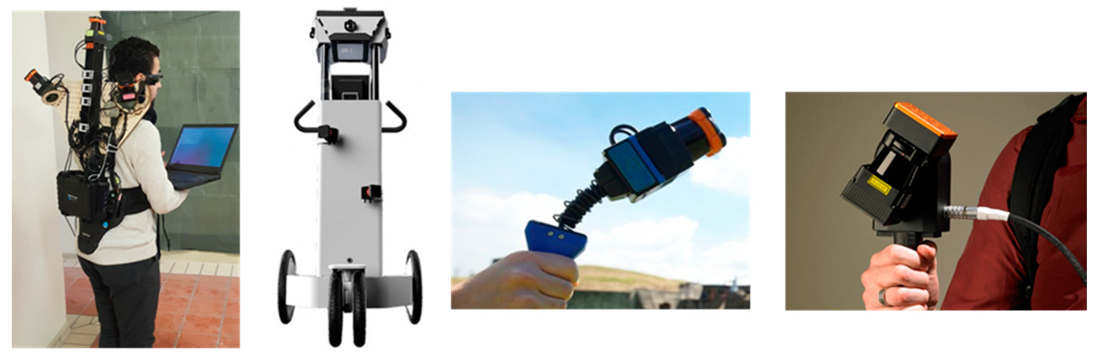
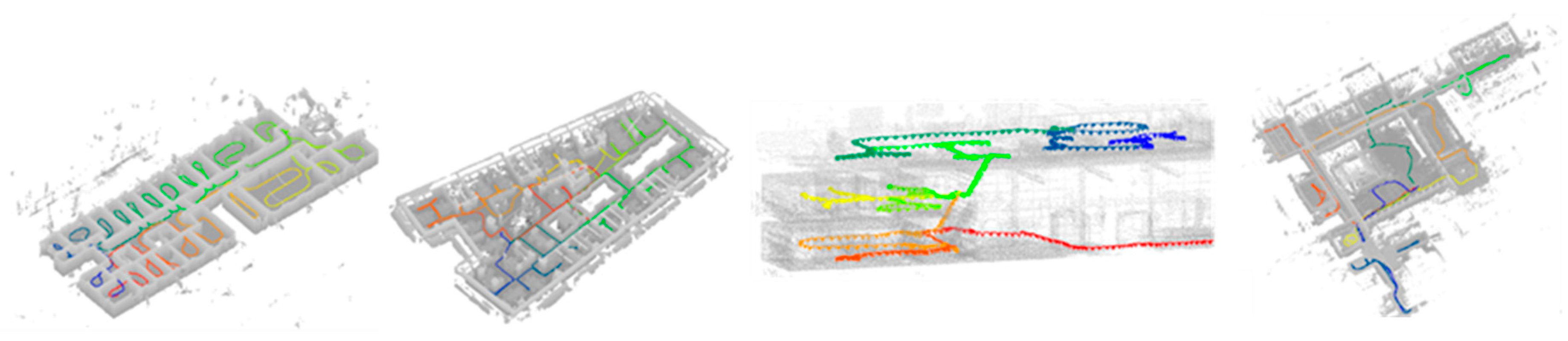
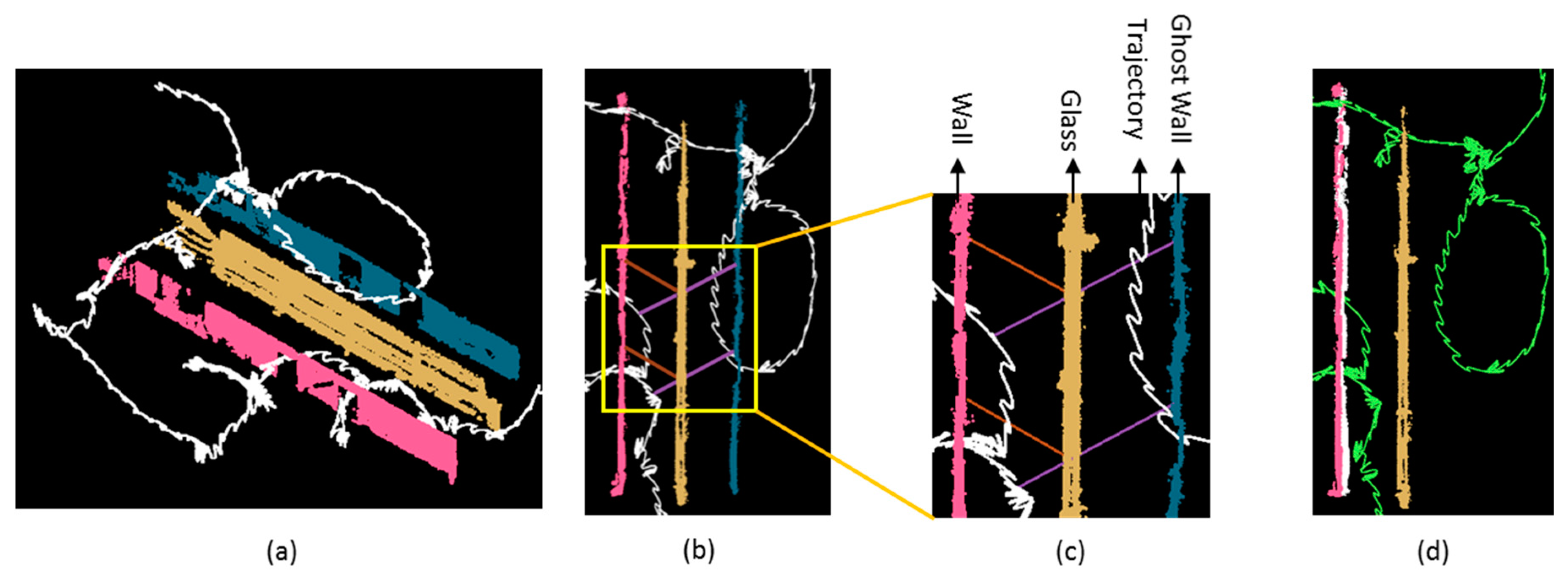
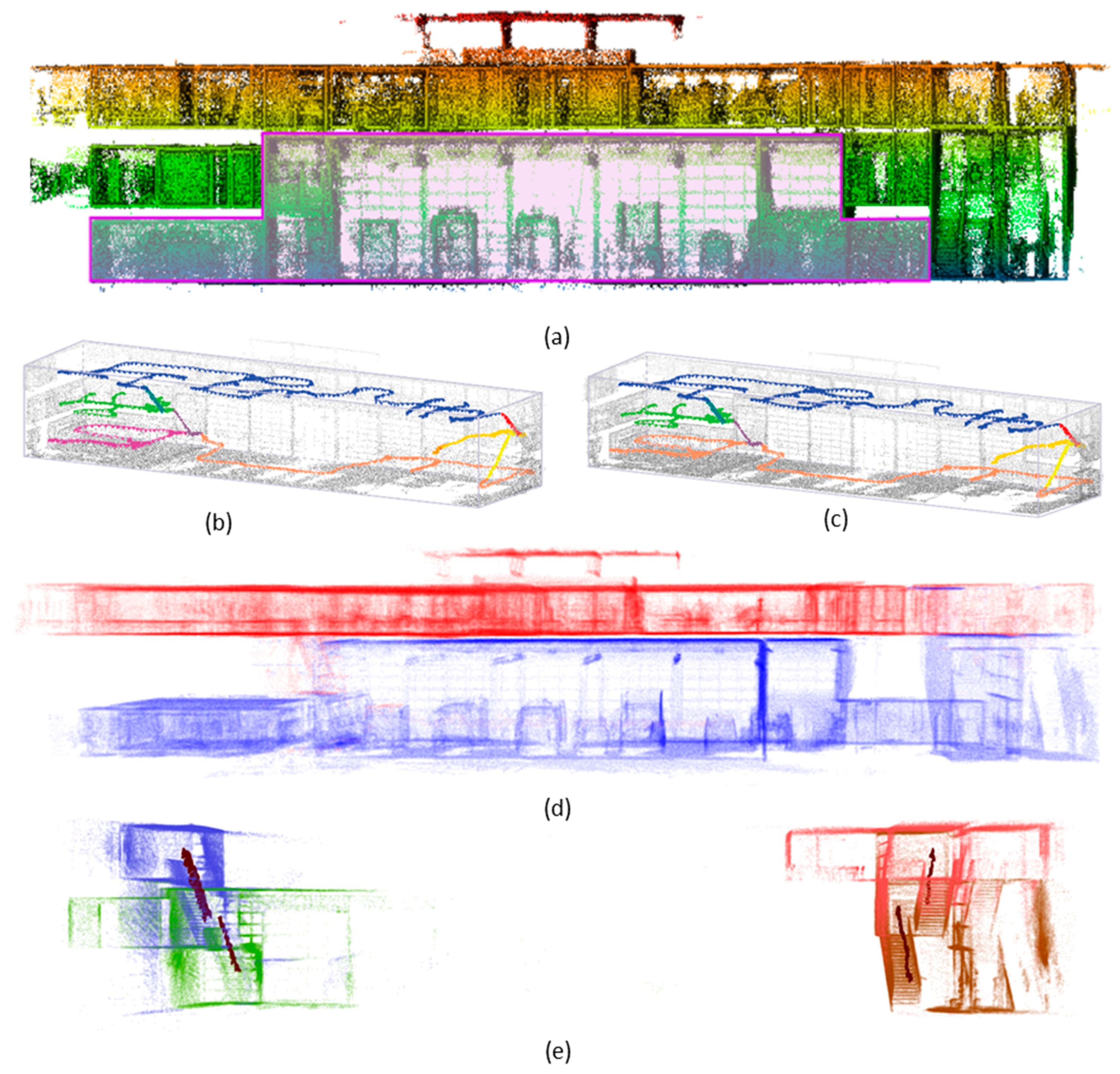
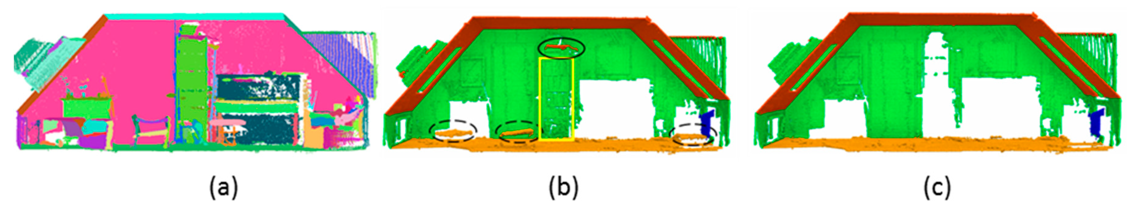
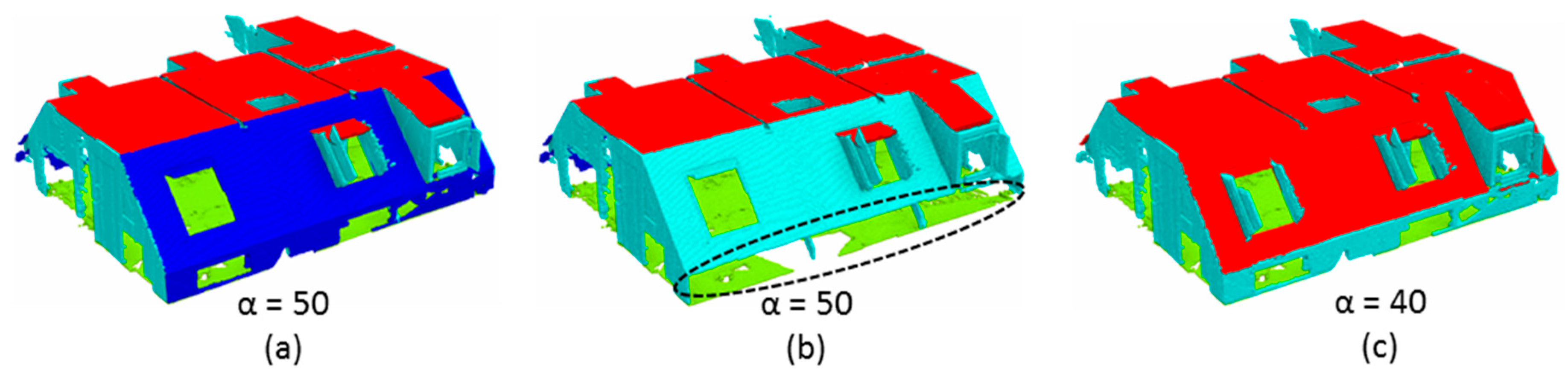
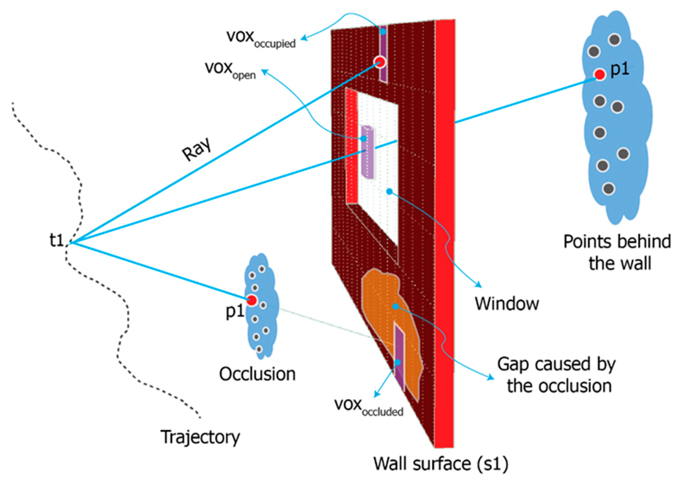
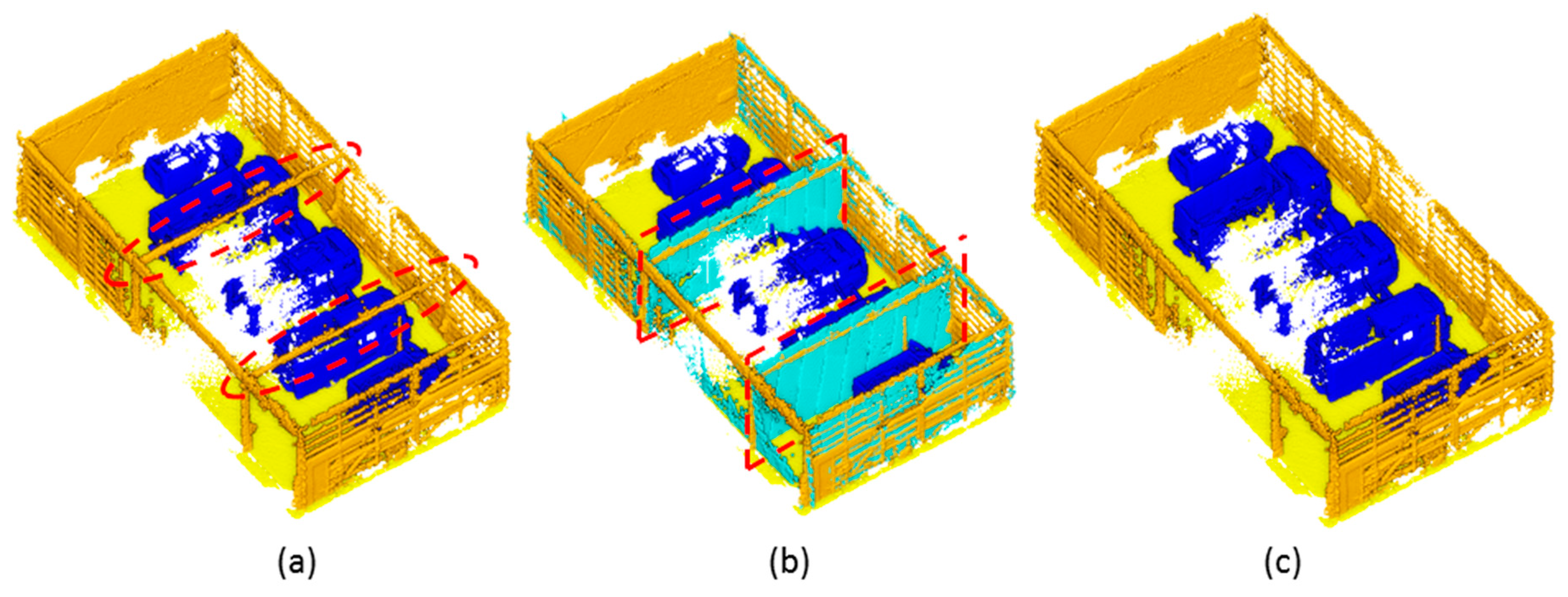
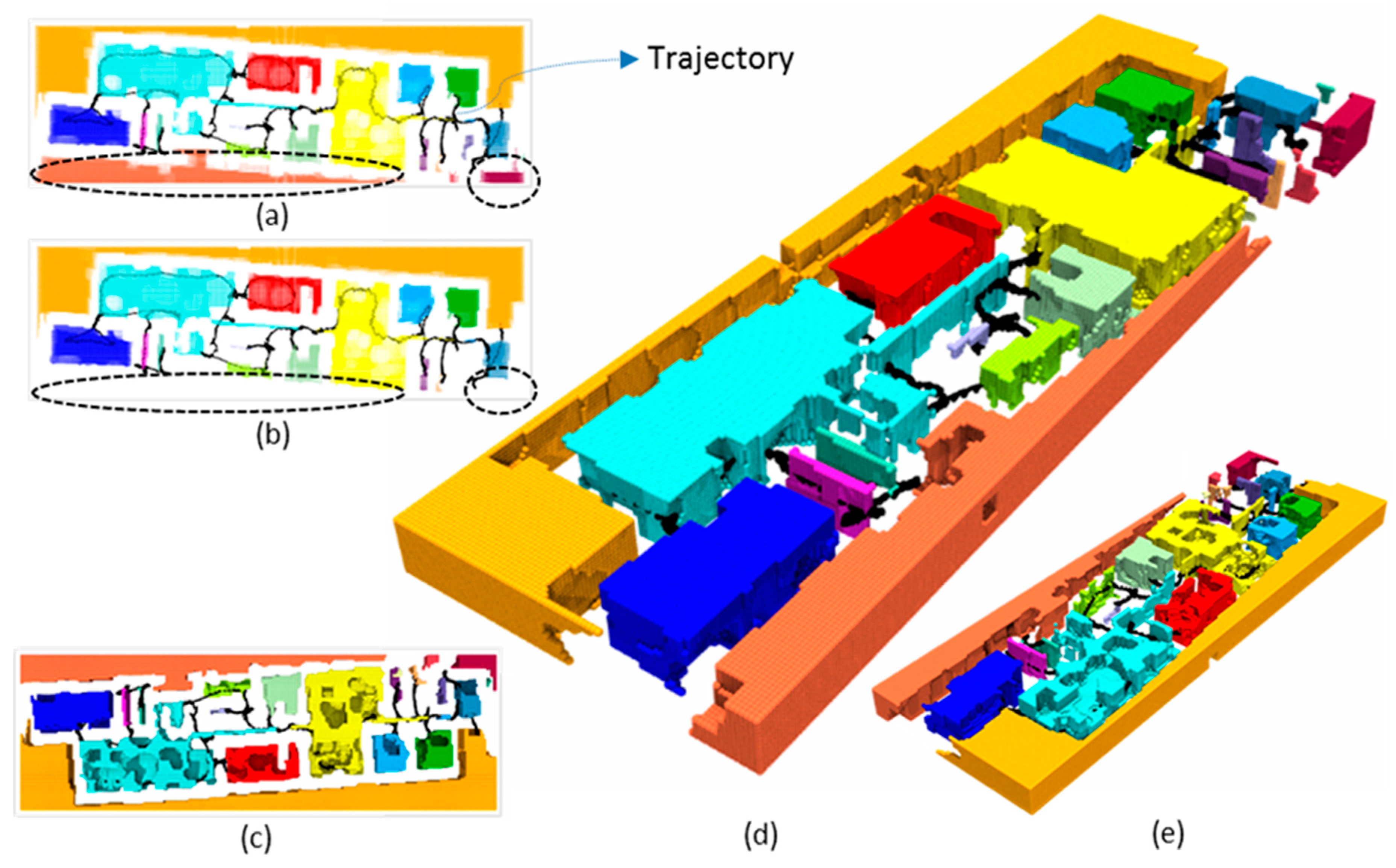
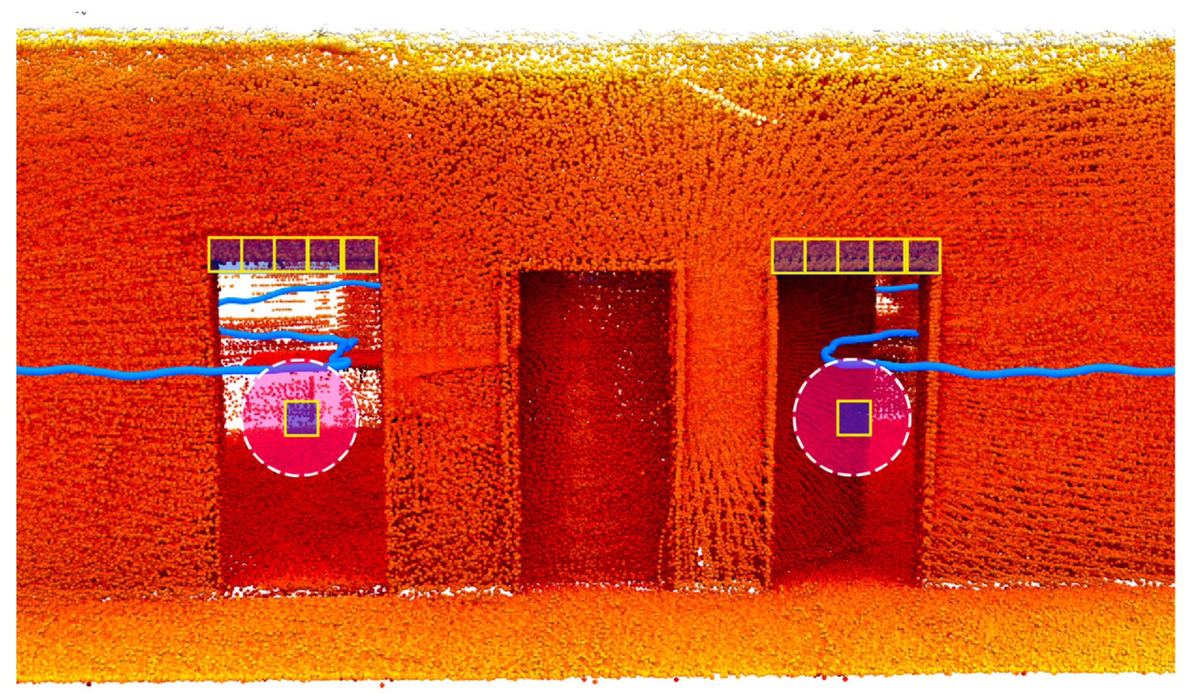
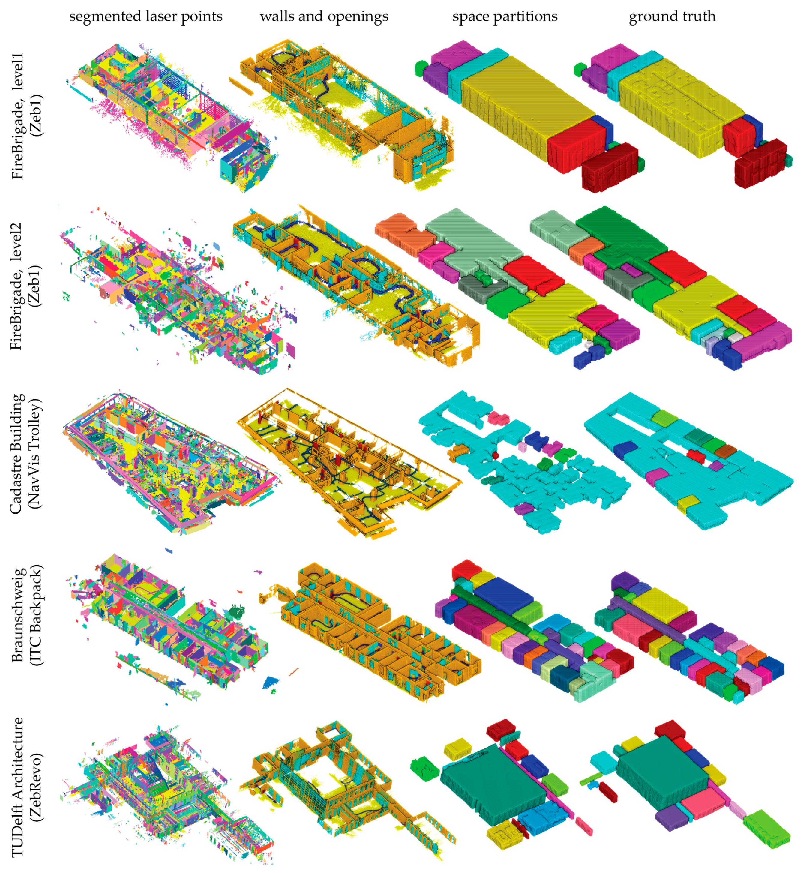
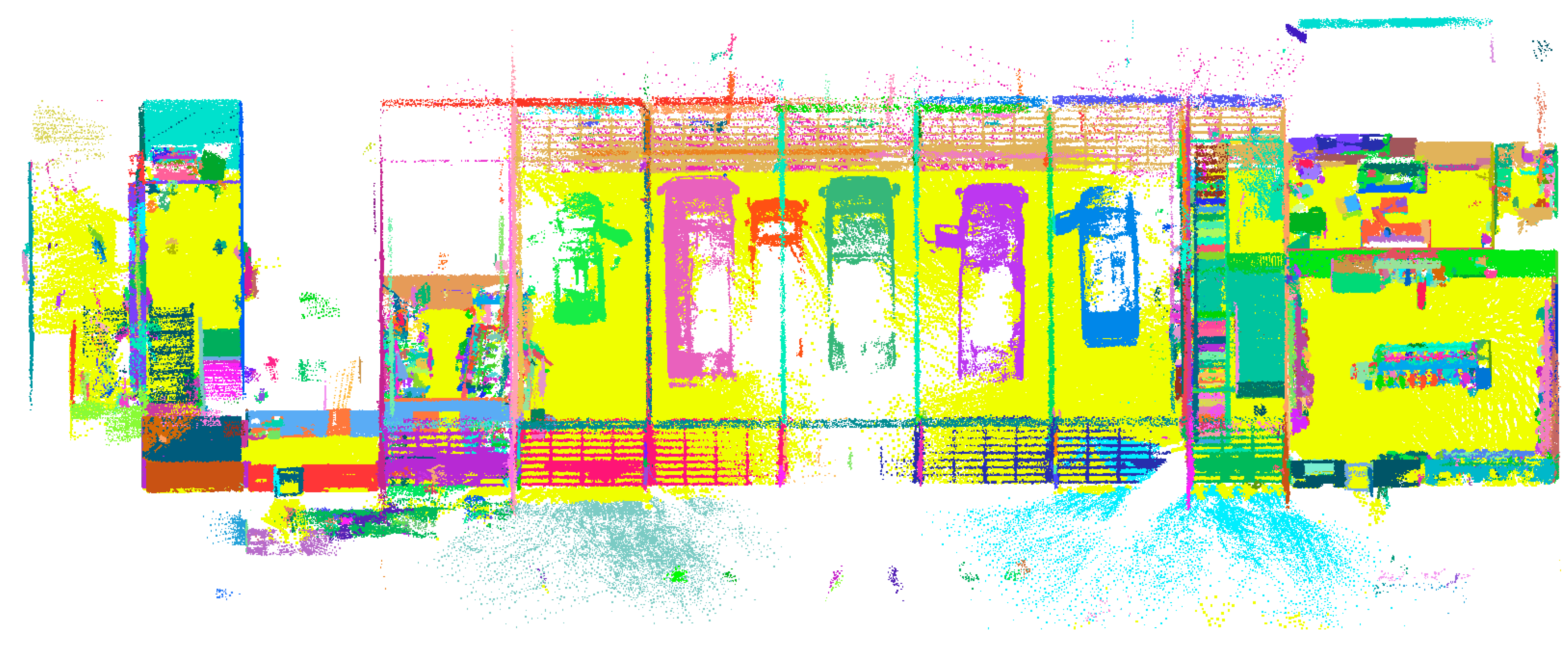
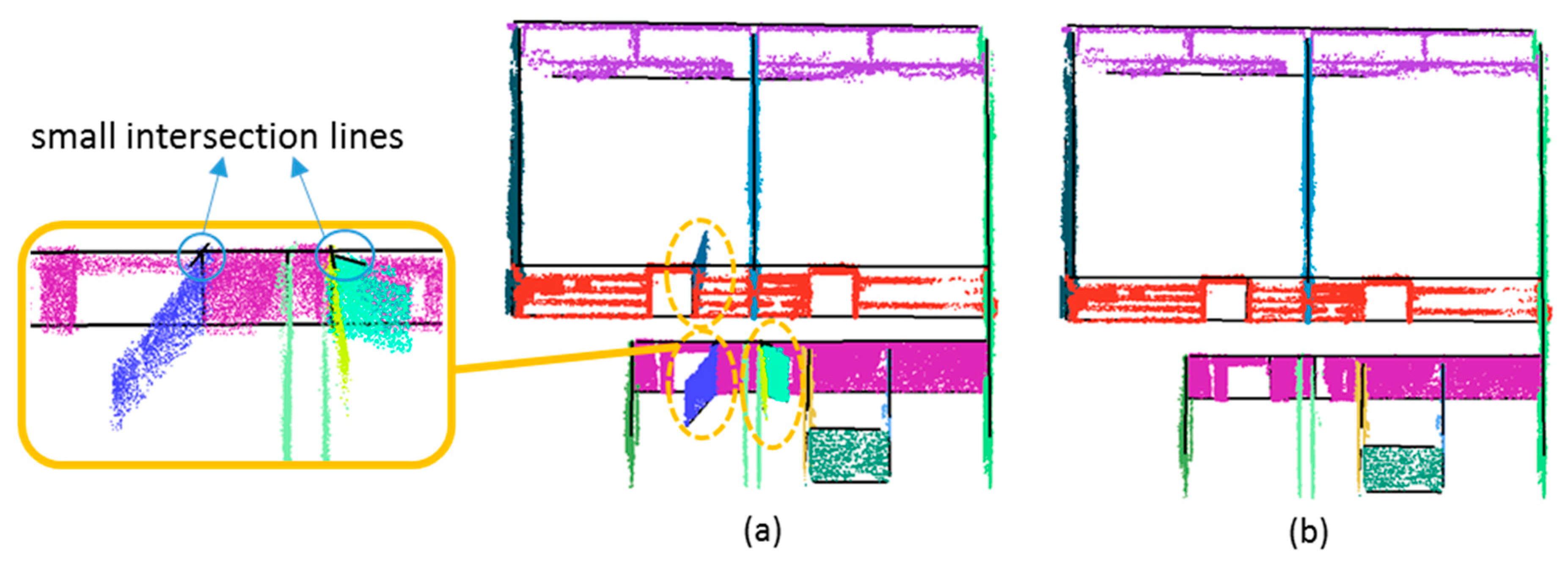
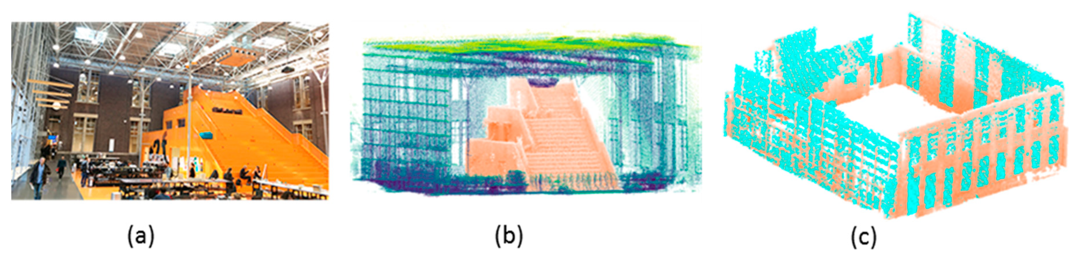
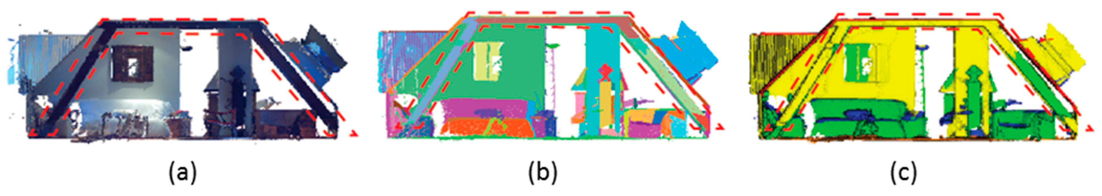
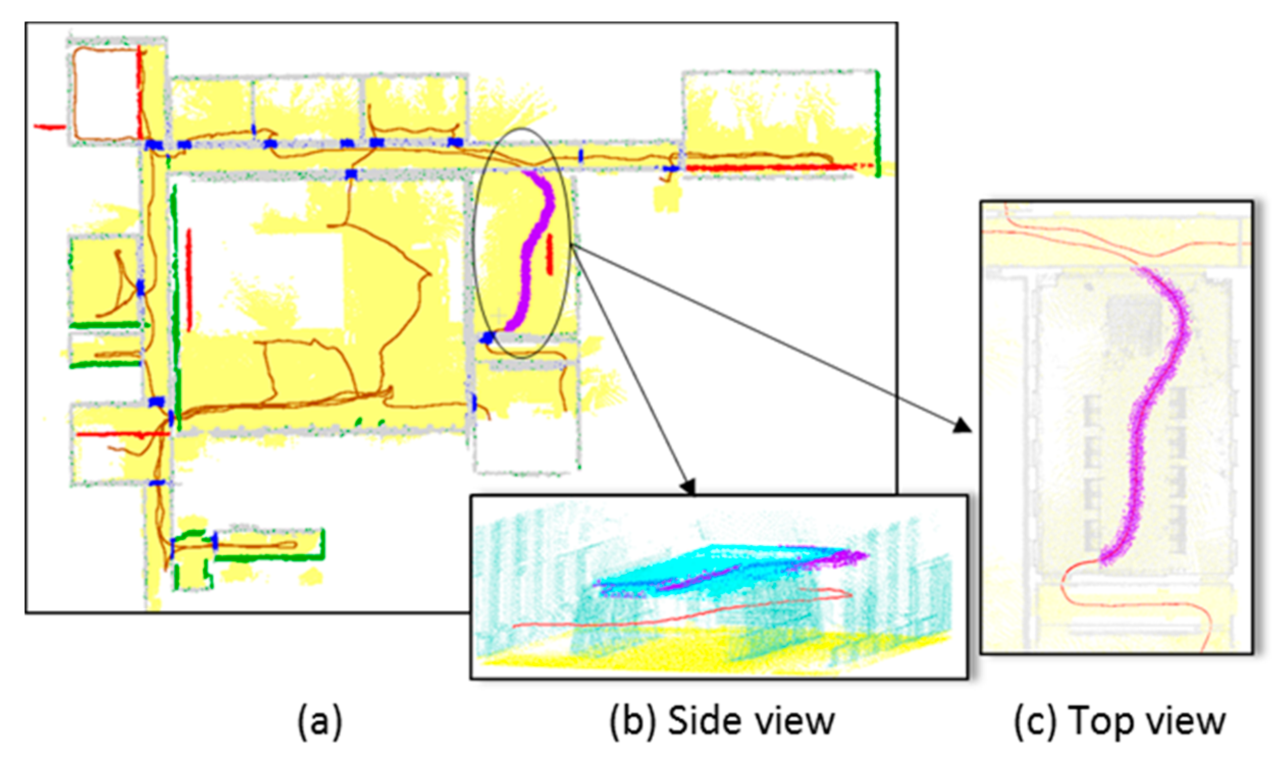
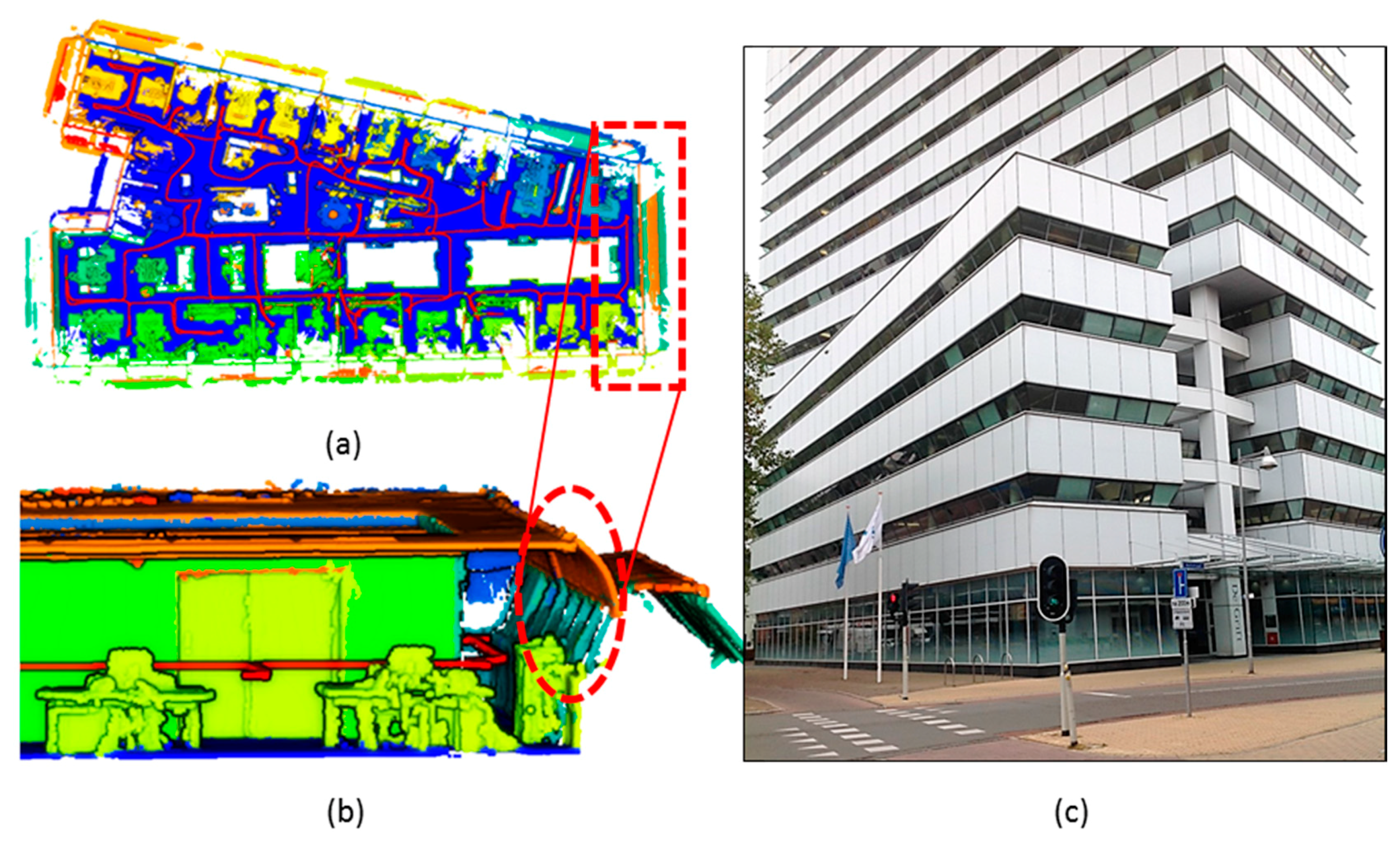
Table 1.
Details of the datasets and capturing device. The number of correctly detected rooms and doors is mentioned in the fourth and fifth columns.
Table 1.
Details of the datasets and capturing device. The number of correctly detected rooms and doors is mentioned in the fourth and fifth columns.
| Dataset | # Points | MLS Device | #Rooms/#Detected | #Doors/#Detected | Clutter and Glass |
|---|---|---|---|---|---|
| Fire Brigade level 1 | 2.9 M | Zeb1 | 9/8 | 8/7 | High |
| Fire Brigade level 2 | 3.6 M | Zeb1 | 16/14 | 17/12 | High |
| Cadastre Building | 4.1 M | NavVis Trolley | 10/9 | 7/5 | High |
| TU Braunschweig | 1.7 M | ITC backpack | 30/27 | 30/29 | Low |
| TU Delft Architecture | 3.2 M | ZebRevo | 18/13 | 25/18 | High |
© 2018 by the authors. Licensee MDPI, Basel, Switzerland. This article is an open access article distributed under the terms and conditions of the Creative Commons Attribution (CC BY) license (http://creativecommons.org/licenses/by/4.0/).
Share and Cite
MDPI and ACS Style
Nikoohemat, S.; Peter, M.; Oude Elberink, S.; Vosselman, G. Semantic Interpretation of Mobile Laser Scanner Point Clouds in Indoor Scenes Using Trajectories. Remote Sens. 2018, 10, 1754. https://doi.org/10.3390/rs10111754
AMA Style
Nikoohemat S, Peter M, Oude Elberink S, Vosselman G. Semantic Interpretation of Mobile Laser Scanner Point Clouds in Indoor Scenes Using Trajectories. Remote Sensing. 2018; 10(11):1754. https://doi.org/10.3390/rs10111754
Chicago/Turabian StyleNikoohemat, Shayan, Michael Peter, Sander Oude Elberink, and George Vosselman. 2018. "Semantic Interpretation of Mobile Laser Scanner Point Clouds in Indoor Scenes Using Trajectories" Remote Sensing 10, no. 11: 1754. https://doi.org/10.3390/rs10111754
Note that from the first issue of 2016, this journal uses article numbers instead of page numbers. See further details here.