Remote Detection of the Fluorescence Spectrum of Natural Pollens Floating in the Atmosphere Using a Laser-Induced-Fluorescence Spectrum (LIFS) Lidar

Abstract

A mobile laser-induced fluorescence spectrum (LIFS) lidar was developed for monitoring pollens floating in the atmosphere. The fluorescence spectrum of pollens excited at 355 nm was measured with a fluorescence spectrometer and the results suggested that in general they had peaks at around 460 nm and the ranges were 400–600 nm. A fluorescence spectrum database of 25 different pollens was made with the 355 nm excitation. Based on these results, we developed a LIFS lidar that had features in pollen species identification and daytime operation. The former was achieved by the database and the latter was possible by introducing a synchronous-delay detection to a gated CCD spectrometer in an operation time of 200 ns. Fluorescence detection of pollens floating in the atmosphere was performed using the LIFS lidar in a field where cedars grow in the spring and ragweed in the autumn. The LIFS lidar system successfully detected fluorescence spectrums of the pollens at a distance of approximately 20 m away. We discussed the performance of the LIFS lidar by estimating the number of cedar pollens using a lidar equation, introducing a fluorescence cross section of cedar pollens and a sensitivity of the CCD spectrometer that was measured by ourselves.

1. Introduction

A very large number of people suffer from a pollen allergy in all regions of the world [1]. In Japan, the main pollens causing allergies are of the Japanese cedar (Cryptomeria japonica) in spring and ragweed (Ambrosia artemisiifolia) in autumn. A survey reported that one fourth of the Japanese population suffers from a cedar pollen allergy [2]. This number will increase when coupled with other factors such as diesel particles from exhausts [3], westernized life styles [4], and the attainment of optimum age of Japanese cedars for pollen production [3]. There is an estimate that climate changes will double the allergy suffering as a result of the doubling of pollens in the year of 2040, compared with 2012 [5]. Thus, the development of pollen monitoring techniques and the delivery of information to the public that urges people to take appropriate action is highly required. The general method of pollen monitoring is by sampling (volumetric and gravimetric) and counting (by manual/automated operations using several optical methods such as scattering, fluorescence, imaging, and so on). For example in Japan, we can check the status of pollen through the Internet monitored by Hanako-san, which is an automated pollen monitoring system operated by the Ministry of Environment of Japan [6]. As monitoring devices are typically set on the ground or on the roofs of buildings, the information gathered is about the particles falling on the ground/roof where the monitoring system is set. Many devices are needed to cover a whole residential area.

On the other hand, pollen can be easily carried by the wind and widely distributed. If the overall process from pollen occurrence, diffusion, transportation, and deposition can be easily monitored by a single system, the benefits will increase. For example, a lidar may predict thunderstorm asthma, which has been happening frequently in Australia [7], by following the pollen behavior together with atmospheric changes. Long distance transports of pollens from North America to Greenland [8], the outer Great Barrier Reef in Australia [9], across the Alps (alt. 2300 m) [10], and others have been reported. These transportations have influenced the earth’s ecosystem and such influences have been deeply connected with our lives besides the pollen allergy problems, in such areas as agriculture, forestry, and fish industries.

A lidar will be a possible candidate for such purpose. It can be used to follow aerosols transportations continuously in time and in ranges that cannot be covered by a point monitoring system. Lidars usually use three different optical interactions, scattering, absorption, and emission. There are several papers inferring the presence of pollen in the atmosphere according to their elastic backscattering (depolarization) data and/or Raman data of lidar observations [11,12,13,14]. Despite the usefulness of the depolarization experiments, the limitations of a scattering lidar are discussed; such as its inability to distinguish and discriminate pollens from other aerosols present in the natural environment [15,16]. On the other hand, it is well known that a large variety of organic materials like pollens can emit their own characteristic autofluorescence (hereafter, fluorescence) [17]. This suggests that fluorescence would be a potential optical interaction for lidar operations having identification capability. Some papers investigated the fluorescence spectrum of bioaerosols, including pollen in a cell/drum experiment [18,19] and lidar performance tests were demonstrated using bioaerosols disseminating in a drum/tunnel/open-air-facility [20]. However, to the best of the authors’ knowledge there are few reports referring to the detection of natural airborne pollens in the atmosphere by a lidar.

In this paper, we report on our experimental results of direct detection of pollen fluorescence spectrum done in a natural field using a LIFS (laser-induced fluorescence spectrum) lidar and discuss the fluorescence spectrum characteristics of pollen, the design and construction of the LIFS lidar, and evaluate the performance by a simple calculation.

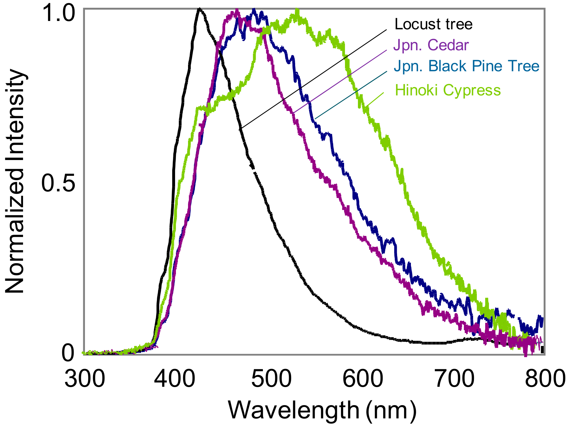
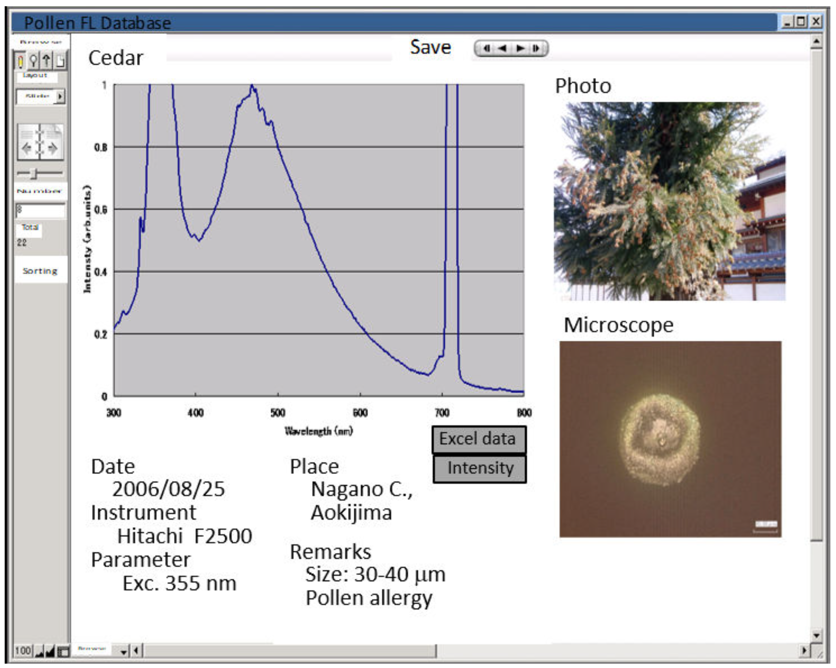
2. Spectral Characteristics of Pollen Fluorescence

To understand the fluorescence characteristics of pollens and to apply them to lidar construction and observations, we measured the fluorescence spectrum of pollens excited at 355 nm. Japanese cedar and Hinoki cypress (Chamaecyparis obtuse) pollens were purchased from a vendor (Miyazo-kahun-kennkyuki, Ibaraki, Japan) and various other kinds of pollens were collected by ourselves from natural plants, orchard trees, and garden flowers. It should be added that we are seeking effective uses of the pollen fluorescence data for agricultural industry although the negative effects only were considered in the previous section. Pollens were stuffed in a quartz window cell and measured by a fluorescence spectrometer (F-2500, Hitachi High-Tech Science Corporation, Tokyo, Japan). The spectral sensitivity of the spectrometer from 200 nm to 600 nm was corrected using Rhodamine B dye in a diffused cell following the manual directions. In Figure 1, we show an example of the fluorescence spectrum of several tree pollens. We made a database of pollen fluorescence (Figure 2) that included 25 varieties using commercial software (FileMaker Pro, FileMaker, Inc., Santa Clara, CA, USA).

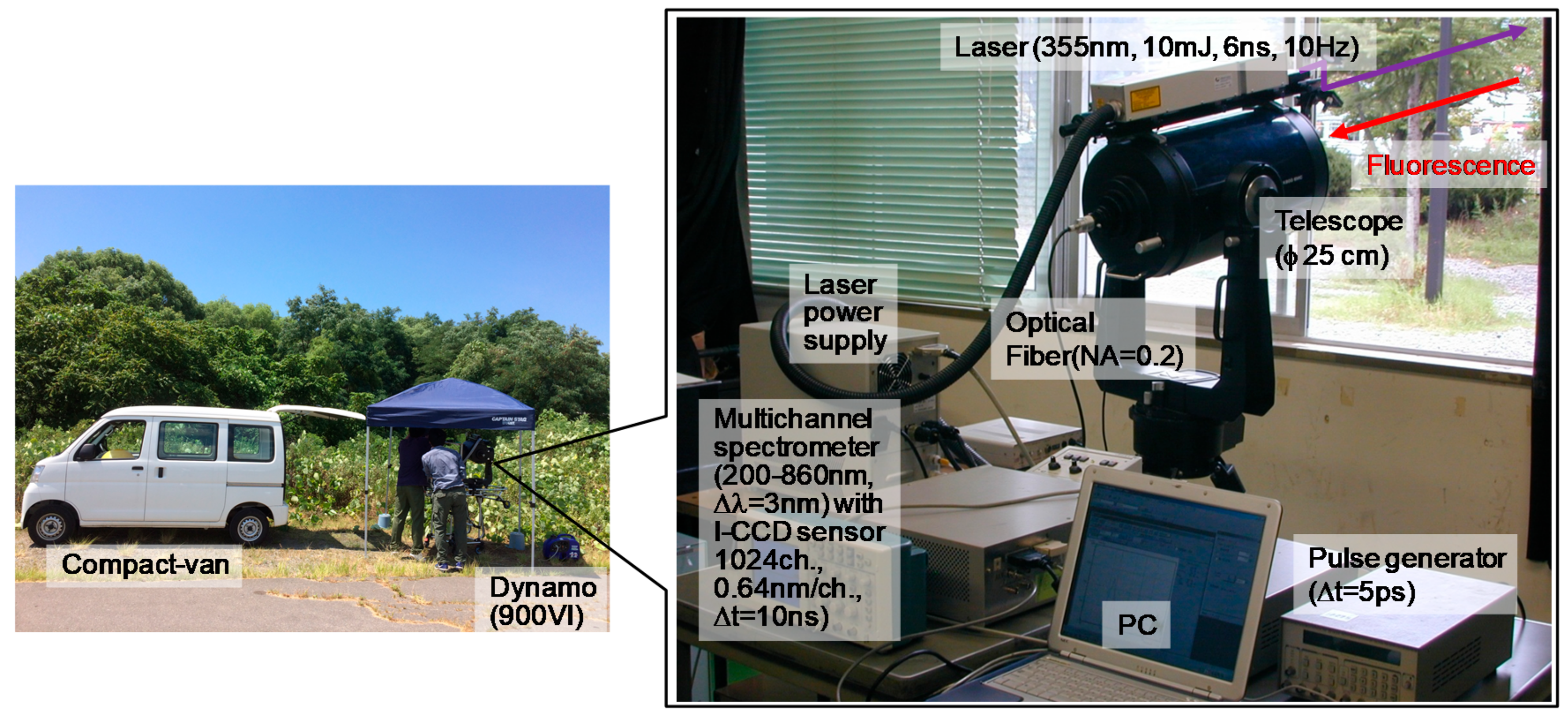
3. LIFS Lidar System

3.1. Design and Construction

We selected cedar pollen in spring and ragweed pollen in autumn for our main LIFS lidar observations, because they are the major species of pollen allergy during each season as described above. In designing the pollen detection lidar, we required two features in the LIFS lidar: (1) pollen species identification that covers the difficulty of traditional elastic backscattering (depolarization) lidars and (2) operation in daytime and at any place because pollen release may be much more active at a warmer temperature after sunrise and pollens are carried freely everywhere by atmospheric convection developing in the daytime.

The LIFS lidar we developed is shown in Figure 3 with some specification details. A pulsed UV YAG laser at 355 nm (Nano L200-10, Litron lasers, Rugby, UK) was used as the lidar source. We prepared a multichannel spectrometer (PMA-11, Hamamatsu, Hamamatsu City, Japan) for the detection, which consisted of a spectrometer (F number 3) and an intensified CCD linear sensor. The sensitivity of the spectrometer was from 200 nm to 860 nm that covers the whole fluorescence spectrum region shown in Figure 1. We expected the LIFS lidar to have the capability of identifying different pollen species by comparing the spectrum patterns of the LIFS lidar results with the fluorescence database.

If we consider the LIFS lidar as a watchdog system that can inform the pollen status in real time to the public and urge them to take some appropriate action, then the pollen lidar observations should be done on a sunny day when pollen release may be highly active and people also are likely to be outside. Otherwise sunny day observations are not suitable for lidar performance because the solar background noise is larger than that in other weather conditions or at night. In the previous reports on fluorescence lidar observation in daytime, observation targets were in high concentration/dense conditions, including hard targets, because it was easier to achieve a signal to noise ratio under such conditions. These observations included plant constituents monitoring [21,22], water quality monitoring [23,24], construction status monitoring [25,26], land monitoring [27], insects [28] and bird [29] detections. The aerosol fluorescence measurement was done only in nighttime [11,30].

We introduced a synchronous-delay detection technique [24] to be able to operate during daytime. If a detector gate opens late during the arrival of a fluorescence emission, because a fluorescence emission is short, the solar background light is significantly decreased. Otherwise the fluorescence signal can be detected synchronously in a short time. The life time of Cedar pollens we measured was about 1–2 ns when they were excited by the YAG laser with a 6 ns pulse width (FWHM). The total width is assumed to be twice, about 12 ns, and the fluorescence emission lasts for 13–14 ns. Therefore, it is preferable to set the CCD gate width around 15 ns. We selected a gated image-intensified CCD (C8808-01S) for the PMA 11. A digital delay/pulse generator (RG535, Stanford Research Systems, Sunnyvale, CO, USA) controlled all the LIFS lidar operations from the laser triggering to gating the CCD with a resolution time of 5 ps.

The laser itself and beam direction mirrors were mounted on a Schmidt-Cassegrainian telescope with a 25 cm diameter (LX200-25, Meade INSTRUMENTS, Irvine, CA, USA), which collected fluorescence. A bundle fiber was set at the focal point of the telescope and delivered fluorescence to the multichannel spectrometer, which performed the detection. The whole system could easily be loaded in a commercial-use compact-van that could be driven even in the narrow and winding roads often found during field observation. The whole LIFS lidar system could be operated with a small dynamo with the power of 900 VI (G900is, Yanmar, Osaka, Japan).

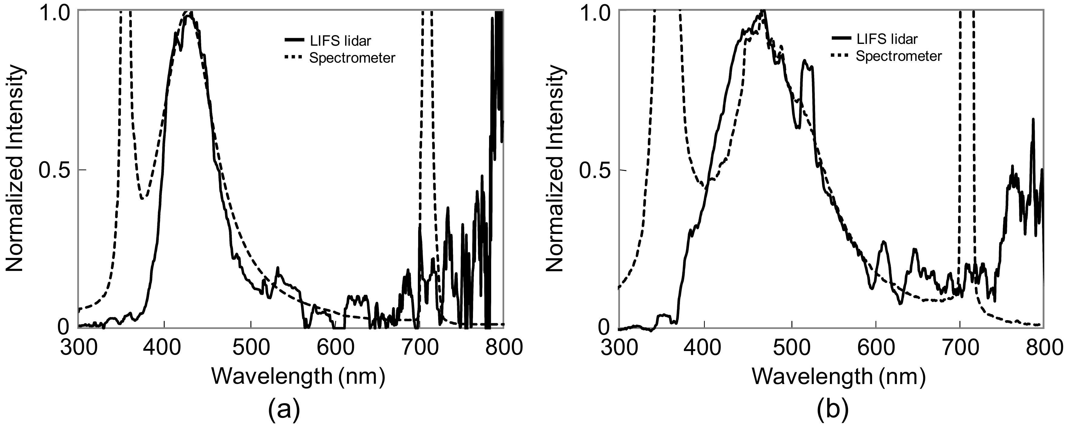
3.2. Performance Check of LIFS Lidar

3.2.1. Detection of False Pollen (Flour Powder)

An air flow device was set on a ladder 20 m away from the LIFS lidar, which consisted of a 40 cm long acrylic pipe with an inner diameter of 20 cm that had two holes of a 8 cm diameter on the long side surface, an air blower under the pipe, and a fan on top of it. Flour powders as false pollens stored in a box were blown up inside the pipe during each run of the LIFS lidar experiment. The LIFS lidar was placed in our laboratory (Figure 3 (right)) and the laser beam was carefully adjusted to pass through the holes. The result shown in Figure 4a depicts a fluorescence spectrum detected by the LIFS lidar and we compare it with the spectrometer reference measurements stored in the database. The operational condition of the LIFS lidar appears in Figure 3 and one spectrum was the averaged value of 100 signals, the measurement time was 10 s. That of the fluorescence spectrometer was that the spectral resolution was 3 nm and the measurement time to cover 200 nm–800 nm was 24 s when the scanning speed of the grating was 1500 nm/min. These conditions were common to Figure 4 and Figure 5.

3.2.2. Detection of Natural Tree Pollen (Japanese Black Pine Tree)

The target for this experiment was Japanese black pine pollens naturally growing in our campus. The LIFS lidar was set on a stretcher and easily carried outside. Electric power was supplied with the generator. The distance between the LIFS lidar and the tree target was about 15 m, with the laser beam passing about 30 cm above the tree. Compared with the result of the flour powder experiment, the fewer number of pollens resulted in a noisier fluorescence spectrum (Figure 4b). However, the experiment suggests the possibility of detection of natural pollens by our LIFS lidar.

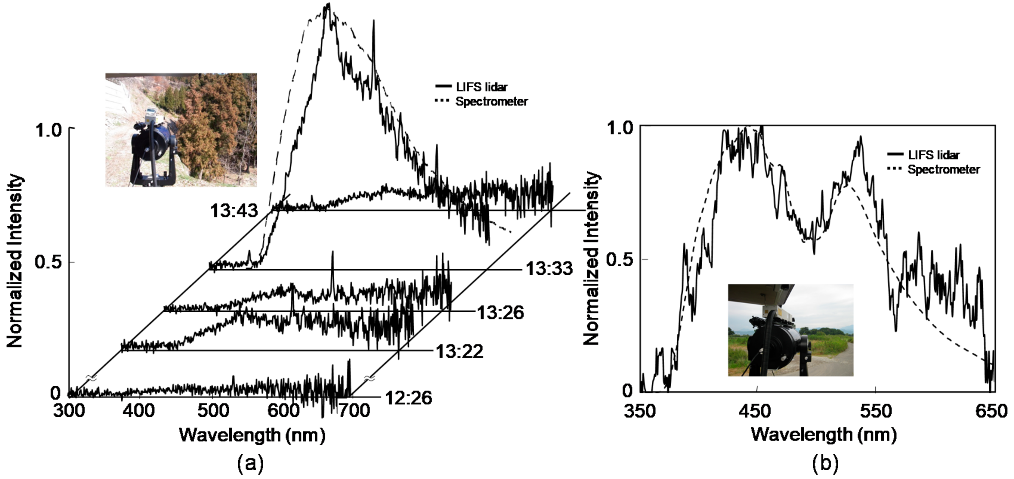
4. Field Observations

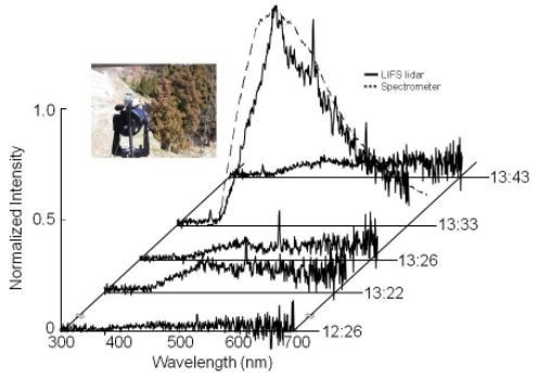
4.1. Cedar Pollen Observations

Spring observations were made at the mountain-side of a town (Matsushiro, Nagano City, Nagano Prefecture, Japan) where a cedar forest had formed, about 20 m (width) × 150 m (length) × 8 m (height). The lidar was placed on the ground so that it was about 3 m higher than the ground of the forest. The distance to the forest was about 20 m and the laser beam passed about 5 m from the end of the forest. The detected fluorescence spectrum is shown in Figure 5a, as well as the spectrum in the database for comparison.

4.2. Ragweed Pollen Observations

Autumn observations were made at a riverbed of a town where the ragweed spread out 500 m along the river in a 200 m width. The laser beam passed horizontally 1 m above the ragweed area. The detected fluorescence spectrum is shown in Figure 5b, which is a running mean value averaged over five successive spectral points (channels) and the spectrum in the database is also given for comparison.

5. Discussions

5.1. System Operations

The database showed that every pollen had its own specific fluorescence spectrum and provides a potential of identification of various pollen species for the LIFS lidar in this work. It should be added that the Excitation-Emission (fluorescence)-Matrix experiments we did show that 355-nm was an applicable wavelength for many aerosol candidate materials, including pollens [31] and EEM itself is much more available for this type of monitoring.

The usefulness of a Nd:YAG laser, a reliable and user-friendly system, was demonstrated in the field studies. A multichannel spectrometer that can cover the whole fluorescence spectrum range over several hundred-nm was necessary to create the spectrum. The synchronous-delay operation of our system was effective in decreasing solar background noise. As the detection period was made shorter, the noise decreased linearly, but the fluorescence signal kept constant in its intensity. The CCD gate time in the field observations was set at 200 ns, which is longer than the fluorescence emission, to compensate for laser jittering occurring around 100 ns. Even in the longer gate times, the effect of the noise reduction was confirmed and daytime observations were successful. The mobile (via compact van) and self-efficient LIFS lidar equipped with a small generator made it possible to conduct environmental monitoring at anytime and at any place without any other infrastructure.

5.2. Pollen Observations in Field

In field experiments, the time dependency of the fluorescence intensity of the cedar pollens was observed. At 12:26, the fluorescence did not appear, then it increased at 13:22, becoming a bit smaller than before at 13:26, and then it reached the peak at 13:33 and there was no pollen detection at 13:43. The lidar could respond to the short-time change in several minutes. The cedars seemed to continuously release pollens, so the increase and decrease in the fluorescence intensity was caused by wind direction, which changed the number of pollens flying into the lidar detection view.

The fluorescence signal of the ragweed pollens was noisy compared to that of the cedar pollens. If the fluorescence efficiency of the ragweed pollens is about the same as the cedar one, it is simply supposed that the number of pollens within the lidar detection view was smaller. The result of the ragweed pollen fluorescence monitoring seems to represent the limitation of our LIFS lidar.

5.3. Estimation of Detected Particle Numbers

We attempted to estimate the number of cedar pollens observed by the LIFS lidar. If we use a lidar equation, we need a fluorescence efficiency of pollen and detector sensitivity.

First, a simple experiment determined the fluorescence efficiency of the cedar pollens. The fluorescence detector was a PMT with an interference filter having a central wavelength of 460 nm and a spectral width of 10 nm. The wavelength matched the peak of the cedar pollen fluorescence. A very small amount of the pollens was placed on a non-fluorescent quartz glass and its number was counted with a particle counter (KC-20, RION, Tokyo, Japan). They were excited by the same laser used for the observations, but the energy was reduced to several hundred micro Joules.

Figure 6 shows the dependency of the PMT output voltage on the number of pollens. The experimental error was about ±4%, most of which was due to the fluctuation of the laser pulse energy. From this, the fluorescence efficiency (fluorescence cross section) of the cedar pollen was calculated as 2 × 10⁻¹⁴ cm² sr⁻¹ nm⁻¹/particle using measurement parameters such as the laser power, PMT voltage, PMT’s sensitivity, divergence formed by the configuration of the laser input and receiver, and the number of pollen. When compared with the cross section of a single particle of pine pollen measured by Stepen that was around 1.7 × 10⁻¹³ cm² sr⁻¹ nm⁻¹/particle at 460 nm with 280-nm excitation [32], there is also an order of magnitude difference between them. The value of the fluorescence cross section varies depending on its species, excitation, and detection wavelengths as we can see in Figure 1. Fluorescence spectrum of pollens of Betula alba, Junglans Nigra, Dactylis Glomerata, and Lycopodium showed a one order magnitude of difference among them even in the same excitation wavelength of 280 nm [33]. In general, biological agents tend to have a stronger fluorescence with shorter excitation wavelengths below 300 nm [18], even in the same species [34]. We concluded the value of fluorescence cross section of cedar pollen obtained can be available in the following discussion.

What we need next is the sensitivity of the multichannel spectrometer PMA-11. Unfortunately, it is not available from the manufacturing company, and the output is displayed as a “count” that may be a value specific to the system itself. On the other hand, lidar systems in general use a PMT detector and measure PMT output voltage (V_PMT) with an oscilloscope. Then we tried a comparative experiment of the PMA detection with the PMT detection.

The experiment was conducted in another LIFS lidar (Figure 7) that we had already set up in our laboratory room and used for the monitoring of atmospheric aerosol fluorescence in which four sets of PMTs with interference filters were changed according to the fluorescence spectral shape of the aerosol we wanted to detect. For the comparative experiment, only one set with 460-nm detection, which is a peak of the Ceder pollen, was needed. A white paper was excited by a 355-nm laser, and the fluorescence at around 460 nm measured by both detection devices was compared.

An input power to both detection devices (P_in (W/nm)) is calculated from the PMT output voltage V_PMT as

P_in = V_PMT/(T_l T_o T_f ∆λ_F S R)

(1)

where T_l and T_f are the transmittance of the lens and the filter, ∆λ_F the bandwidth of the filter, T_o optical efficiency of optical components other than the lens and the filter, S the anode sensitivity of the PMT, and R output resistance of PMT. The PMA sensitivity (count/nm) that is a ratio of monitoring power (P_PMA (count/nm)) using the PMA to that (P_in) using the PMT are expressed using a conversion factor η (count/W)

P_PMA = P_in η

(2)

The comparative experiment resulted in that η was 1.5 × 10¹⁰ (count/W).

Table 1. Calculation Parameters.

	Parameter	Symbol	Value
For PMA sensitivity calculation	Transmittance of lens	Tl	92%
	Optics efficiency	To	93%
	Transmittance of filter	Tf	92%
	Filter spectral width	ΔλF	10 × 10−9 (m)
	PMT anode sensitivity	S	4.4 × 101 (A/W) at −300 (V)
	Resistance	R	50 (Ω)
	PMT output	VPMT	21.42 × 10−3 (V) at −300 (V)
	PMA output	PPMA	53376 (count/3 nm) at gain 8
For pollen number calculation	Laser power	P	10 × 10−3 (/6 ns)
	Fluorescence cross section of Cedar pollen	σ	2 × 10−18 (m2 sr−1 nm−1)
	Overlapping factor	Y	1
	Telescope effective area	A	0.045 (m2)
	Range	r	20 (m)
	Velocity of light	c	3 × 108 (m/s)
	Laser pulse width	tL	6 × 10−9 (s)
	Atmospheric transmittance of laser	TL	0.992 (km−1) at 355 nm for visibility of 20 km [35]
	Atmospheric transmittance of fluorescence	TF	0.995 (km−1) at 460 nm for visibility of 20 km [36]
	PMA output	PPMA	320 (count/3 nm) at gain 8

shows parameters used for the calculation in which P_PMA and V_PMT were given by the comparative experiment.

Following a lidar equation, P_in is as

P_in = P Nσ YA/r² (cτ_L/2)T_LT_D,

(3)

where P is the laser power, N the pollen density, σ the fluorescence cross section of the pollen, Y the overlap factor, A the effective telescope area, c the velocity of light, τ_L laser pulse width, T_L atmospheric transmittance of the laser, and T_F atmospheric transmittance of the fluorescence. Thus, the number of the pollen received by the PMA detector is estimated as follows;

N = P_PMA/{ηPσ YA/r² (Cτ_L/2) T_LT_D}.

(4)

We could calculate the observed particle number of the LIFS lidar as 2.2 × 10⁷ (particle/m³) at 20 m. The parameters for the calculation are listed in Table 1, in which P_PMA was given by the observation.

The number monitored by Hanako-san at the Amori Office of the Nagano Environmental Conservation Research Institute (Amori, Nagano City, Nagano Prefecture, Japan) fluctuated severely 0-several 100 particles/m³ with sudden increase up to 2000 (particles/m³) [6]. The institute is located in a residential area about 7 km away from the cedar pollen observation site. It appears that the higher calculated number of the LIFS lidar observation is due to the proximity to the origin of the pollens just released and the fact that the pollens have not yet spread into a larger space. The pollens were gathered in a limited space, so spectral intensity was strongly affected by the wind direction as seen in Figure 5. The measurements by the Amori Office are lower because the pollens have had time to diffuse during transportation. For example, if the number of 2.2 × 10⁷ (particle/m³) spreads into an even 100 m × 100 m × 100 m area, it will be diluted to 22 (particle/m³).

To use the LIFS lidar as a watchdog system, it is important to predict the direction to where pollen will float as well as the number. Therefore, the information should be obtained in the air close to the source before it moves to and falls on a residential area. Pollen in the air can be freely carried and change the direction of the transportation in several minutes as shown in the field experiment. The LIFS lidar system can respond to those requests.

6. Conclusions

We investigated fluorescence lidar for pollen monitoring. We still need comparative experiments between the LIFS lidar monitoring and a point monitoring using a particle counter at the same location and time. However, field experiments of the fluorescence spectrum detection of cedar and ragweed pollens confirmed that the LIFS lidar is a potential apparatus for this type of monitoring, even in daytime.

We have two plans for further developing the LIFS lidar. One is the construction of a watchdog system that will quickly deliver information. Our LIFS lidar takes 10 s to get one measurement of data. If we average 100 signals using a 10 Hz laser, which needs several minutes to process and save data manually, we can obtain the fluorescence spectrum every 4–10 min, as shown in Figure 5a. We have already succeeded in delivering LIFS lidar data to a personal mobile phone from an observation place directly using a commercial communication system [24]. On the other hand, the gravitational method using a Durham’s sampler that has been used as a traditional and basic method of pollen particle counting needs to one day inform the pollen status to the public. A more advanced one is the volumetric method using a particle counter based on the principle of optical scattering. Hanako-san, introduced in the introduction, is a particle counter. The pollen count is loaded up every hour on its website.

The other plan is to develop it into a scanning lidar, which will allow us to make a three-dimensional (cross-sectional structure with range resolution) map of pollen distribution. We have started the basic experiments with fluorescence monitoring of trees [31].

References

1. Pollen Allergy-Australasian Society of Clinical Immunology and Allergy (ASCIA). Available online: https://www.allergy.org.au/patients/allergic-rhinitis-hay-fever-and-sinusitis/pollen-allergy (accessed on 17 August 2018).
2. Baba, K.; Nakatsu, K. National epidemiological survey of nasal allergy in 2008. Prog. Med. 2008, 28, 145–156. (In Japanese) [Google Scholar]
3. Ishizaki, T.; Koizumi, K.; Ikemori, R.; Ishiyma, Y.; Kushibiki, V. Studies of prevalence of Japanese cedar pollinosis among the residents in a densely cultivated area. Ann. Allergy 1987, 58, 265–270. [Google Scholar] [PubMed]
4. Saito, Y. Japanese Cedar Pollinosis: Discovery, Nomenclature, and Epidemiological Trends. Available online: https://www.jstage.jst.go.jp/article/pjab/90/6/90_203/_article (accessed on 24 September 2018).
5. American College of Allergy. Asthma and Immunology, The Year 2040: Double the pollen, Double the Allergy Suffering. Available online: https://acaai.org/news/year-2040-double-pollen-double-allergy-suffering (accessed on 24 September 2018).
6. Pollen Monitoring System. Available online: http://kafun.taiki/go/jp (accessed on 17 August 2018). (In Japanese).
7. Lee, J.; Kronborg, G.; O’Hehir, R.E.; Hew, M. Who’s risk of thunderstorm asthma? The ryegrass pollen trifecta and lessons learnt from the Melbourne thunderstorm epidemic. Respir. Med. 2017, 132, 46–148. [Google Scholar] [CrossRef] [PubMed]
8. Rousseau, D.D.; Schevin, P.; Ferrier, J.; Jolly, D.; Andreasen, T.; Ascanius, S.E.; Hendriksen, S.E.; Poulsen, U. Long-distance pollen transport from North America to Greenland in spring. J. Geophys. Res. 2008, 113, G02013. [Google Scholar] [CrossRef]
9. Moss, P.T.; Kershaw, A.P.; Grindrod, J. Pollen transport and deposition in riverine and marine environments within the humid tropics of northeastern Australia. Rev. Palaeob. Palyn. 2005, 134, 55–69. [Google Scholar] [CrossRef] [Green Version]
10. Frei, T. Pollen distribution at high elevation in Switzerland: Evidence for medium range transport. Grana 1997, 36, 34–38. [Google Scholar] [CrossRef] [Green Version]
11. Immler, F.; Engelbart, D.; Schrems, O. Fluorescence from atmospheric aerosol detected by a lidar indicates biogenic particles in the lower stratosphere. Atmos. Chem. Phys. 2005, 5, 345–355. [Google Scholar] [CrossRef]
12. Noh, Y.M.; Lee, H.; Mueller, D.; Lee, K.; Shin, D.; Shin, S.; Cho, T.J.; Choi, Y.J.; Kin, K.R. Investigation of the diurnal pattern of the vertical distribution of pollen in the lower troposphere using LIDAR. Atmos. Chem. Phys. 2013, 13, 7619–7629. [Google Scholar] [CrossRef] [Green Version]
13. Cao, X.; Roy, G.; Bernier, R. Lidar polarization discrimination of bioaerosols. Opt. Eng. 2010, 49, 116201. [Google Scholar]
14. Sassen, K. Boreal tree pollen sensed by polarization lidar: Depolarizing biogenic chaff. Geophys. Res. Lett. 2008, 35, L18810. [Google Scholar] [CrossRef]
15. Yee, E.; Kosteniuk, P.R.; Roy, G.; Evans, B.T.N. Remote biodetection performance of a pulsed monostatic lidar system. Appl. Opt. 1992, 31, 2900–2913. [Google Scholar] [CrossRef] [PubMed]
16. Simard, J.R.; Roy, G.; Mathieu, P.; Larochelle, V.; McFee, J.; Ho, J. Standoff sensing of bioaerosols using intensified range-gated spectral analysis of laser-induced fluorescence. IEEE Trans. Geosci. Remote Sens. 2004, 42, 865–874. [Google Scholar] [CrossRef]
17. Wolfbeis, O.S. The Fluorescence of Organic Natural Products. In Moleculaar Luminescence Spectroscopy; Schulman, S.G., Ed.; John Wiley & Sons: New York, NY, USA, 1985. [Google Scholar]
18. Pohlker, C.; Huffman, J.A.; Poschl, U. Autofluorescence of atmospheric bioaerosols-fluorescent biomolecules and potential interferences. Atmos. Meas. Tech. 2012, 5, 37–71. [Google Scholar] [CrossRef] [Green Version]
19. Pan, Y.L. Detection and characterization of biological and other organic-carbon aerosol particles in atmosphere using fluorescence. J. Q. Spec. Radiat. Transfer 2015, 150, 12–35. [Google Scholar] [CrossRef]
20. Carrano, J.C.; Collins, C.J. (Eds.) Optically Based Biological and Chemical Detection for Defence V. Proc. SPIE 2009, 7484. [Google Scholar] [CrossRef]
21. Cerovic, Z.G.; Samson, G.; Morales, F.; Tremblay, N.; Moya, I. Ultraviolet-induced fluorescence for plant monitoring: present state and prospectis. Agronomie 1999, 19, 543–578. [Google Scholar] [CrossRef]
22. Saito, Y. Laser-induced fluorescence spectroscopy/technique as a tool for field monitoring of physiological status of living plants. Proc. SPIE 2007. [Google Scholar] [CrossRef]
23. Pisano, A.M.; Dominicis, D.; Biamino, W.; Bignami, F.; Gherardi, S.; Colao, F.; Coppini, G.; Marullo, S.; Sprovieri, M.; Trivero, P.; et al. An oceanographic survey for oil spill monitoring and model forecasting validation using remote sensing and in situ data in the Mediterranean sea. Deep-Sea Res II 2016, 133, 132–145. [Google Scholar] [CrossRef]
24. Saito, Y.; Kakuda, K.; Yokoyama, M.; Kubota, T.; Tomida, T.; Park, H.D. Design and daytime performance of laser-induced fluorescence spectrum lidar for simultaneous detection of multiple components, dissolved organic matter, phycocyanin, and chlorophyll in river water. Appl. Opt. 2016, 55, 6727–6734. [Google Scholar] [CrossRef] [PubMed]
25. Weibring, P.; Johansson, T.; Edner, H.; Svanberg, S.; Sundner, B.; Raimondi, V.; Cecchi, G.; Pantani, L. Fluorescence lidar imaging of historical monuments. Appl. Opt. 2001, 40, 6111–6120. [Google Scholar] [CrossRef] [PubMed]
26. Raimondi, V.; Cecchi, G.; Lognoli, D.; Palombi, L.; Gronlund, R.; Johansson, A.; Svanberg, S.; Barcup, K.; Hallstorm, J. The fluorescence lidar technique for the remote senseing of photoautotrophic biodeteriogens in the outdoor cultural heritage: A decade of in situ experiments. Intern. Biodet. Biodeg. 2009, 63, 823–835. [Google Scholar] [CrossRef]
27. Hodge, F.E.; Swift, R.N.; Yungel, J.K. Feasibility of airborne detection of laser-induced fluorescence emissions from green terrestrial plants. Appl. Opt. 1983, 22, 2991–3000. [Google Scholar] [CrossRef]
28. Brydegaard, M.; Guan, Z.; Wellenreuther, M.; Svanberg, S. Insect monitoring with fluorescence lidar techniques: feasibility study. Appl. Opt. 2009, 48, 5668–5677. [Google Scholar] [CrossRef] [PubMed]
29. Brydegaard, M.; Lundin, P.; Guan, Z.; Runemark, A.; Akesson, S.; Svanberg, S. Feasibility study: fluorescence lidar for remote bird classification. Appl. Opt. 2010, 49, 4531–4544. [Google Scholar] [CrossRef] [PubMed]
30. Sugimoto, N.; Huang, Z.; Nishizawa, T.; Matsui, I.; Ttatarov, B. Fluorescence from atmospheric aerosols observed with a multi-channel lidar spectrometer. Opt. Exp. 2012, 20, 20800–20807. [Google Scholar] [CrossRef] [PubMed]
31. Saito, Y.; Tomida, T.; Shiraishi, K. Fluorescence lidar seamlessly connecting individual observation of the globl environmental systems. Proceedings of Lidar Remote Sensing for Environmental Monitoring XVI, Honolulu, HI, USA, 24–25 September 2018. [Google Scholar]
32. Stepens, J.R. Fluorescence cross section measurements of biological agent simultants. In Proceedings of the 1996 Edgewood RDEC Scientific Conference on Obscuration and Aerosol Research, Aberdeen, MD, USA, 19–22 November 1996. [Google Scholar]
33. Weichert, R. Determination of backscatter and fluorescence cross-sections of biological aerosols. Landb. Volk. 2002, 34, 83–87. [Google Scholar]
34. Reiner, W.; Klemm, W.; Legenhausen, K.; Pawellek, C. Determination of backscatter and fluorescence ross section of biological aerosols. Part. Syst. Charact. 2002, 19, 216–222. [Google Scholar]
35. Baum, W.A.; Dunkelman, L. Horizontal attenuation of ultraviolet by the lower atmosphere. J. Opt. Soc. Amer. 1995, 45, 166–174. [Google Scholar] [CrossRef]
36. Bertolotti, M.; Mluzii, L.; Sette, D. On the possibility of measuring optical visibility by using a Ruby laser. Appl. Opt. 1969, 8, 117–120. [Google Scholar] [CrossRef] [PubMed]
Figure 1. Fluorescence spectrum of several tree pollens excited at 355 nm.
Remotesensing 10 01533 g001
Figure 2. Display image of fluorescence database which includes information such as pollen name, images, experiment conditions (measurement system, date, place etc.), and comments. Headings are in Japanese.
Remotesensing 10 01533 g002
Figure 3. Photographs of the laser-induced fluorescence spectrum (LIFS) lidar (right) and the field experiment (left).
Remotesensing 10 01533 g003
Figure 4. Flour fluorescence spectrum (a) and Jpn. red pine fluorescence spectrum (b) measured by the LIFS lidar.
Remotesensing 10 01533 g004
Figure 5. Detection of fluorescence spectrum of Jpn. Cedar pollen (a) and Ragweed pollen (b) in the air by the LIFS lidar.
Remotesensing 10 01533 g005
Figure 6. PMT output voltage depending on the number of pollens.
Remotesensing 10 01533 g006
Figure 7. Configuration of comparative experiment, the PMA detection with the PMT detection. M: mirror. DM: dichroic mirror, IF: interference filter.
Remotesensing 10 01533 g007