Typhoon/Hurricane-Generated Wind Waves Inferred from SAR Imagery


1
School of Marine Sciences, Nanjing University of Information Science and Technology, Nanjing 210044, China
2
Department of Oceanography, Dalhousie University, Halifax, NS B3H 4R2, Canada
3
Fisheries and Oceans Canada, Bedford Institute of Oceanography, Dartmouth, NS B2Y 4A2, Canada
4
Department of Engineering Mathematics and Internetworking, Dalhousie University, Halifax, NS B3H 4R2, Canada
*
Authors to whom correspondence should be addressed.
Remote Sens. 2018, 10(10), 1605; https://doi.org/10.3390/rs10101605
Submission received: 29 August 2018
/
Revised: 5 October 2018
/
Accepted: 5 October 2018
/
Published: 9 October 2018
(This article belongs to the Special Issue Sea Surface Roughness Observed by High Resolution Radar)
Abstract
:The wide-swath mode of synthetic aperture radar (SAR) is a good way of detecting typhoon/hurricane winds with a cross-polarization mode. However, its ability to detect wind waves is restricted because of its spatial resolution and nonlinear imaging mechanisms. In this study, we use the SAR-retrieved wind speed, Sentinel-1 SAR wave mode and buoy data to examine fetch- and duration-limited parametric models (denoted H-models), to estimate the wave parameters (significant wave height Hs, dominant wave period Tp) generated by hurricanes or typhoons. Three sets of H-models, in total 6 models, are involved: The H-3Sec model simulates the wave parameters in 3 sections of a given storm (right, left and back); H-LUT models, including the H-LUTI model and H-LUTB model, provide a better resolution of the azimuthal estimation of wind waves inside the storm by analyzing the dataset from Bonnie 1998 and Ivan 2004; and the third set of models is called the H-Harm models, which consider the effects of the radius of the maximum wind speed rm on the wave simulation. In the case of typhoon Krovanh, the comparison with wave-mode measurements shows that the duration-limited models underestimate the high values for the wind-wave Hs, while the fetch models’ results are more accurate, especially for the H-LUTI model. By analyzing 86 SAR wave mode images, it is found that the H-LUTI model is the best among the 6 H-models, and can effectively simulate the wind-wave Hs, except in the center area of the typhoon; root mean square errors (rmse) can reach 0.88 m, and the coefficient correlation (R2) is 0.86. The H-Harm models add rm as an additional factor to be considered, but this does not add significant improvement in performance compared to the others. This limitation is probably due to the fact that the data sets used to develop the H-Harm models have only a limited coverage range, with respect to rm. Applying H-models to RADARSAT-2 ScanSAR mode data, we compare the retrieved wave parameters to collected buoy measurements, showing good consistency. The H-LUTI model, using a fetch-limited function, does the best among these 6 H-models, whose rmse and R2 are 0.86 m and 0.77 for Hs, and 1.06 s and 0.76 for Tp, respectively. Results indicate the potential for H-models to simulate waves generated by typhoons/hurricanes.
1. Introduction
Wind-waves generated by extreme weather, such as typhoons or hurricanes, are among the most important dynamic elements of the marine environment [1,2,3,4,5]. A well-known example is the Perfect Storm in October 1991, which is sometimes known by wave researchers as the Halloween Storm, which generated maximum waves in excess of 30 m [6]. The development of remote sensing has greatly motivated the studies of large storm waves [7,8,9], as in situ observations are spatially sparse and expensive undertakings [10,11,12,13]. Because of its ability to make measurements under almost all weather conditions, day or night, synthetic aperture radar (SAR) is an important way to monitor marine winds and waves.
Over the past decades, studies concerning SAR wave detection and the inversion algorithm methodologies have achieved some developments. Originally, Hasselmann et al. (1991) suggested a wave spectrum inversion algorithm for SAR imaging of waves [14]. On the basis of that approach, many successive nonlinear wave spectral algorithms were proposed, such as SPRA (Semi-Parametric Algorithm) [15], PFSM (Parameterized First-guess Spectrum Method) [16,17,18] and PARSA (Partition Rescaling and Shift Algorithm) [19]. These algorithms need to build a first guess wave spectrum, based on the additional wave information, which might be provided by a numerical wave model or parametric wave spectrum model. However, because SAR imaging of ocean waves is affected by nonlinear imaging mechanisms causing distortion of shorter waves [20,21], it is difficult to observe short wind waves, which is a key problem in observations of storm-generated waves.
Instead of using an image-to-wave spectra inversion scheme, alternative approaches were developed to empirically estimate integral wave parameters, such as significant wave heights or wave periods, from SAR images. CWAVE_ERS [21] and CWAVE_ENVI [22] are empirical models for ERS-2 and Envisat ASAR wave mode images. Based on the Sentinel-1 SAR wave mode, Stopa et al. proposed CWAVE-S1A and Fnn models to retrieve significant wave heights and dominant wave periods by using cut-off wavelength and other SAR image parameters [23]. The imaging range of the SAR wave mode is quite small (~20 km), making it impractical for large-scale monitoring of a wide range of observations of storm generated waves. Alternatively, ScanSAR mode images have a larger swath-width for observations, for example as much as 500 km for RADARSAT-2, making it applicable for monitoring large scale fields of storm winds and waves. However, its low spatial resolution, ranging from 60–100 m for RADARSAT-2, limits its observational ability for short wind waves [24,25,26,27].
Despite the complicated spatiotemporal distribution characteristics of the wind fields associated with storms, many studies show that most of measured 1-D wave spectra under storms are monomodal and suggest that the associated surface waves follow the same similarity concept as the waves that grow in response to steady winds in fetch-limited conditions [28,29,30,31,32]. Young [29] suggested that the nonlinear wave-wave interactions play a central role in stabilizing the shape of unimodal spectrum [33,34]. This is achieved by the transfer of wave energy within the spectrum, from high frequencies to low frequencies, and the other way around, from low to high frequencies [35,36], although the wind input and dissipation by breaking may also be important at this stage of wave growth [11,31,37]. Many parametric models were built on the assumption of the fetch-limited condition, particularly in the 1970s and 1980s [38], providing a rapid means to explore the general characteristics of waves generated by storms, especially the asymmetry of the wave field [39,40,41] and energy [32] inside the storms. Based on the fetch- or duration-limited wind wave growth relations, Hwang et al. [42,43,44] proposed three sets of wind wave models for storms, denoted as the H-models, which use the wind field to estimate the significant wave heights Hs and dominant wave periods Tp directly for the wind waves. Parameters of the wind waves can be estimated in three separate sectors (left, right, and back) of the storm by the H-3Sec model [42]. After analyzing more wind and wave spectral data generated by hurricanes and collected by the Scanning Radar Altimeter (SRA), Hwang and Walsh [43] proposed the H-LUT model, which provides a better azimuthal resolution for estimating the wind wave parameters inside storms. In addition, by considering the influence of the radius of maximum storm winds on the wave estimation, Hwang and Fan [44] further developed the H-Harm models.
At present, SAR has been widely applied for observations of typhoon wind fields, especially the cross-polarization SAR [45,46,47,48,49,50] which appears to be able to largely resolve the signal saturation problem at high winds, experienced in co-polarization SAR and scatterometer observations [51]. Therefore, by combing the relatively accurate storm winds determined from cross-polarization SAR measurements, with the H-models, it is possible to obtain the wind waves generated by typhoon and hurricane environments.
The remainder of the paper is organized as follows: Section 2 describes the Sentinel-1 SAR wave mode, RADARSAT-2 ScanSAR mode and the fetch- and duration-limited wind wave models (H-models). Section 3 shows the detailed validations of H-models for estimating significant wave heights for typhoon Krovanh and other typhoons using Sentinel-1 SAR wave mode wind and wind-wave data. By combing the buoy wave data and RADARSAT-2 ScanSAR mode winds, the H-models are applied to estimate significant wave heights and dominant wave periods for six additional hurricanes. Discussion follows in Section 4, and Conclusions in Section 5.
2. Data and Methods
2.1. Sentinel-1 SAR Wave Mode
Sentinel-1 (S1A) Level-2 Ocean Products, OCN, can provide wind speed and significant wave height from SAR wave mode. Significant wave heights for wind waves are calculated from the nonlinear part of the SAR image through the cross spectrum methodology [52] combined with the SPRA inversion algorithm [15]. S1A was launched on April 2014 and was the first satellite with a SAR observation system among the ESA Sentinel series. The S1A SAR wave mode was put into service in July 2015 for observations of waves over the global ocean. This SAR wave mode has 4 m spatial resolution, with a small imaging range (20 km × 20 km). In addition, S1A operates in the C-Band at two incidence angles, 23° and 36°, alternating along the satellite orbital direction at 100 km intervals. Thus, the S1A SAR wave mode can provide almost continuous sampling, collecting abundant simultaneous wind and wave measurements under storm conditions.
2.2. RADARSAT-2 ScanSAR Mode
RADARSAT-2 is a C-band spaceborne SAR, which was launched on 14 December 2007. The satellite has the capability to provide single-, dual- and quad-polarization SAR imaging mode data, day or night, in almost all-weather, with multi-spatial resolution of the sea surface. We focus on measurements from RADARSAT-2 cross-polarization ScanSAR mode, which provides wide swath (450 km) images and has a pixel spacing of 50 m, which is high potential for hurricane/typhoon monitoring over a relatively large spatial scale.
The wind speeds used to calculate waves are retrieved by the C-2POD (C-band cross-polarized ocean surface wind retrieval model) model [46]. The wind speed range of the fit for C-2POD is 3.7–39.7 m/s, which is an important motivation for using C-2POD to retrieve the wind speeds from dual-polarization SAR images. The model was previously validated against SFMR measurements and H*wind, and the comparisons showed good agreement.
2.3. The Fetch- and Duration-Limited Wind Wave Models (H-Models)
According to recent studies, the fetch- and duration-limited wind wave growth relations derived from steady wind forcing conditions appear to be applicable for waves generated by typhoon/hurricane winds [28,29,30,31,32,33,34,35,36,37,38,39,40,41], which conforms the essential role of nonlinear wave-wave interactions in maintaining the shape of wave spectrum. Based on this assumption, Hwang et al. successively proposed three sets of models for wind waves generated by hurricanes [42,43,44], which are summarized here. The fetch- and duration-limited wind wave growth relations, in terms of the dimensionless variance and dimensionless frequency as functions of significant wave height Hs and wave period Tp, can be represented as equations of dimensionless fetch :
where , , dimensionless fetch is and wind speed at 10 m height is U10. In the same way, the equations of dimensionless duration are:
where dimensionless duration is . The xf and td are fetch and duration respectively. All of the parameters in (1) and (2) above are the functions of wind-wave triplets: Hs, Tp and U10. Substituting these relations into Equations (1) and (2) leads to
and
As shown by these equations, given fetch xf or duration td, Hs and Tp can then be directly calculated from the wind field U10. Wave height and wave period calculated from the fetch-limited growth functions are denoted by FHs and FTp respectively. Wave height and wave period calculated from duration-limited growth functions are denoted by DHs and DTp respectively.
The key to estimating wind-wave information with these growth relations is to first determine the fetch and duration. For a finite water body with a well-defined land-water interface, the fetch and duration can be defined easily according to their definitions. However, it is difficult to directly obtain fetch and duration under inhomogeneous or unsteady wind situations, like storms. By making use of Equations (3) or (4), the equivalent fetch and equivalent duration inside the typhoon/hurricane can also be obtained from the wind-wave triplets. Based on SRA (Scanning Radar Altimeter) measurements of Hs, Tp and U10, Hwang et al. [42,43,44] proposed three groups of typhoon/ hurricane fetch and duration models. They are:
(1) H-3Sec model
Using 60 wave spectra of hurricane Bonnie (1998), Hwang [42] gives the empirically formulas in terms of the fetch (unit: km) and duration (unit: h) for the three sectors of the storm (left, right, back). They are functions of the radial distance r (unit: km) from the hurricane center
The subscripts , , and indicate the variables derived from the equations for , respectively. This model is hereafter denoted as the H-3Sec model.
(2) H-LUT model
Hwang and Walsh [43] analyzed the full set of the SRA wave measurements collected during hurricane Bonnie (1998), which contains 233 spectra along 10 transect flights radiating from the hurricane center, and improved the ability of the H-3Sec model to simulate surface waves in the azimuthal and radial directions under storms. The fetch and duration relations are represented as
The slopes and intercepts in the equations are functions of azimuth angle , which is referenced to the direction of the hurricane motion. The convention is that the angles are positive counterclockwise. Similarly, an alternative set of empirical coefficients is obtained through analyzing the data from hurricane Ivan (2004). The corresponding parametric models above are denoted as the ‘H-LUTB’ model and ‘H-LUTI’ model, respectively.
(3) H-Harm model
By considering the influence of the radius of the maximum wind speed in storms in the fetch- and duration-limited simulations, the third set of models was proposed [44]. Similar to the H-LUT model, fetch and duration are also expressed with radial components r and , like Equations (7) and (8). The slope and intercept can be decomposed as Fourier series,
where q represents the slopes and the intercepts . The harmonic parameters and exhibit a systematic quasi-linear variation with the radius of maximum wind speed,
where Y represents amplitudes
and ; and and are empirical coefficients. Given the storm wind field, and can be calculated by Equation (10), using the radius of maximum wind speed rm. Inserting these variables into Equation (9), the slopes and intercepts in Equations (7) and (8) can be computed. Thus, with the wind speed input, we can determine the equivalent fetches and durations for any point inside the storms by (7) and (8).
Please note the value of N in the Fourier series (9) might affect the results. We denote the models with N = 1, 2, 3 as ‘H-Harm1’, ‘H-Harm2’, and ‘H-Harm3’ respectively. In addition, because of the lack of wave period data in S1A Level-2 products, we can only make comparisons with the significant wave heights for typhoon/hurricane–generated waves using wind measurements of S1A SAR wave mode data.
3. Results
3.1. Validation of H-Models by Sentinel-1A SAR Wave Mode Wind and Wave Data
3.1.1. Typhoon Krovanh
Between 14 and 21 September 2015, Sentinel-1A (S1A) tracks passed over typhoon Krovanh (2015) three times, acquiring 17 SAR wave mode images (Figure 1a). On 14 September, Krovanh proceeded to the east of the Mariana Islands, and then moved northwest. As S1A moved along its descending track on 15 September, S1A captured 6 SAR wave mode images of Krovanh. Because this acquisition occurred within a minute, the measurements of the SAR wave mode images can be regarded as instantaneous sampling relative to the typhoon time scales. The corresponding typhoon center is shown as a red cross in Figure 1a, and the radius of maximum wind speed and the maximum wind speed are 61.7 km and 21.4 m/s, respectively, at that moment. Under the typhoon reference frame (Figure 1b), it is shown that the SAR measurements occurred in the rear portions of both the left and right regions. As Krovanh continued to move northwest, the maximum wind speed continued to increase, up to 33 m/s on 16 September. Thereafter, S1A captured additional four SAR images around Krovanh. The sampling areas are located on the right side of the typhoon. The maximum wind speed reached 40.1 m/s, with radius reduced to 27 km, while the air-sea exchange remained relatively strong. The last sampling by S1A of typhoon Krovanh occurred on September 20, as the typhoon began to dissipate. At that time, the maximum wind speed decreased to 20.6 m/s and the radius increased to 74.08 km. The typhoon track, maximum wind speed and radius of maximum wind speed are provided by the Join Typhoon Warning Centre (JTWC).
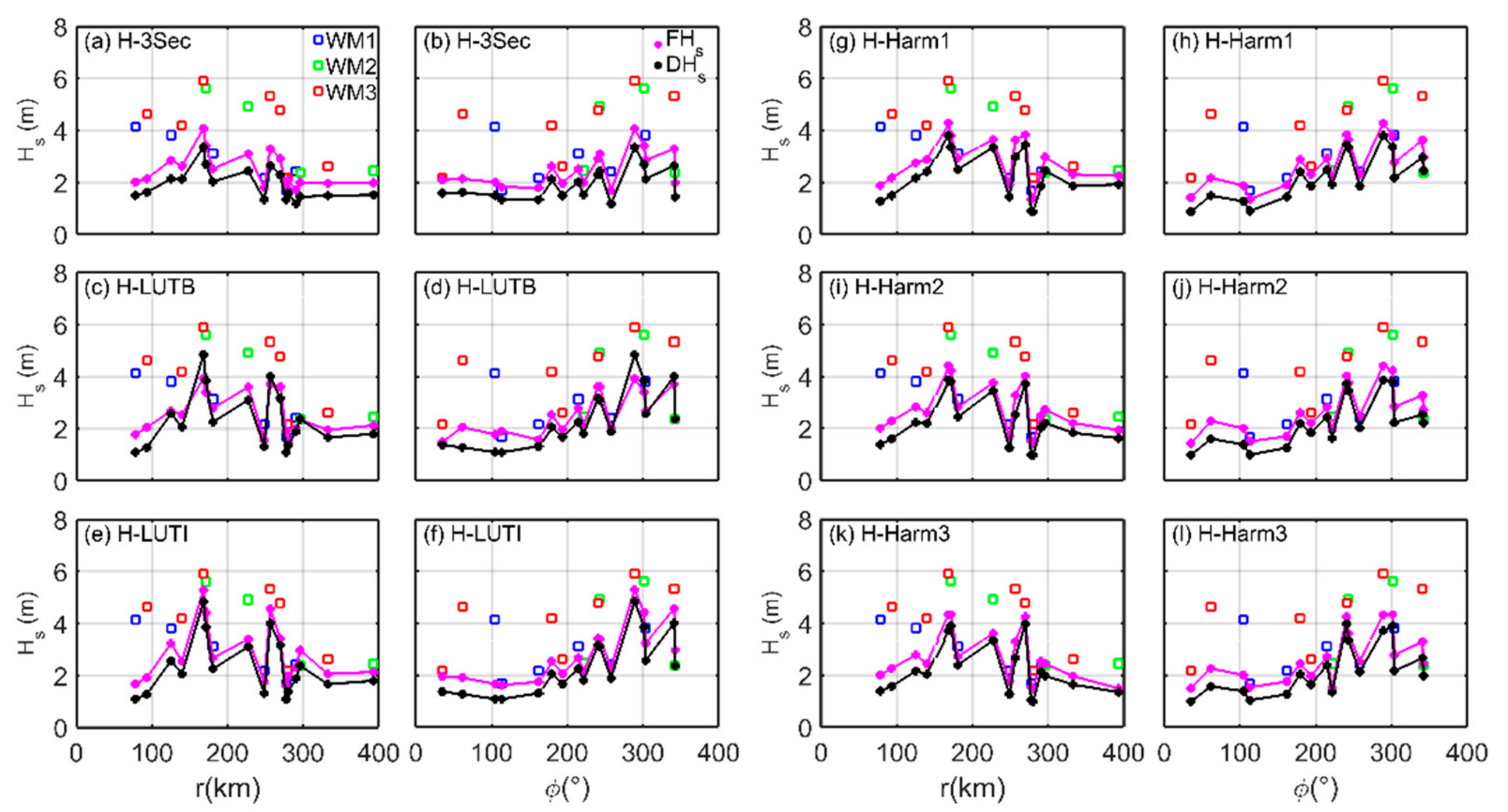
By comparing H-model simulation results (FHs and DHs) to significant wave heights from S1A Level-2 products (Figure 2), it is found that Hs is underestimated to different extents by each model. Values from fetch models FHs are typically slightly larger than those from duration models DHs, and are closer to those measured by S1A. Each H-model has a better performance for the simulation of Hs less than 5 m. However, these models have large differences when simulating regions where the high waves dominate. In particular, estimates from the H-3Sec model seriously underestimate Hs in cases larger than 4 m. Secondly, the set of H-Harm models all have similar simulation performances, although in regions of higher significant wave heights, results from H-Harm2 and H-Harm3 appear to perform slightly better than the simulation by the H-Harm1 model. We conclude that the H-LUT models work best in these sets of models; and the H-LUTI model is clearly better than the H-LUTB model.
In Figure 2, the measurements by S1A are marked with three different colors (of squares), corresponding to those shown in Figure 1a (1st pass: Blue; 2nd pass: Green; 3rd pass: Red), which occurred at different stages of the typhoon development: Generation stage, full maturity stage and decay stage. The highest values of Hs occurred during the typhoon decay stage. Accordingly, the deviations in simulations for these H-models are largest during this stage. Although the maximum wind speed and radius of maximum wind speed during the generation stage are quite similar to those during the collapse of the typhoon, the values for Hs in this former stage are relatively smaller. Of course, this follows the processes that form the growth and development of the waves as the storm progresses through the stages of its life cycle. Thus, the performance of the Hs simulation models is good during the generation stage. The main areas with large deviations are near the radius of maximum wind speed (r = 78.19 km, ). Previous studies [53] have shown that wider angles between wind and wave propagation directions are always in the left regions of the typhoon, which indicates that the wave field is dominated by swell. However, H-modes are based on the wind-wave growth relationships, which perform poorly in the left regions of the typhoons.
3.1.2. 12 Pacific Typhoons
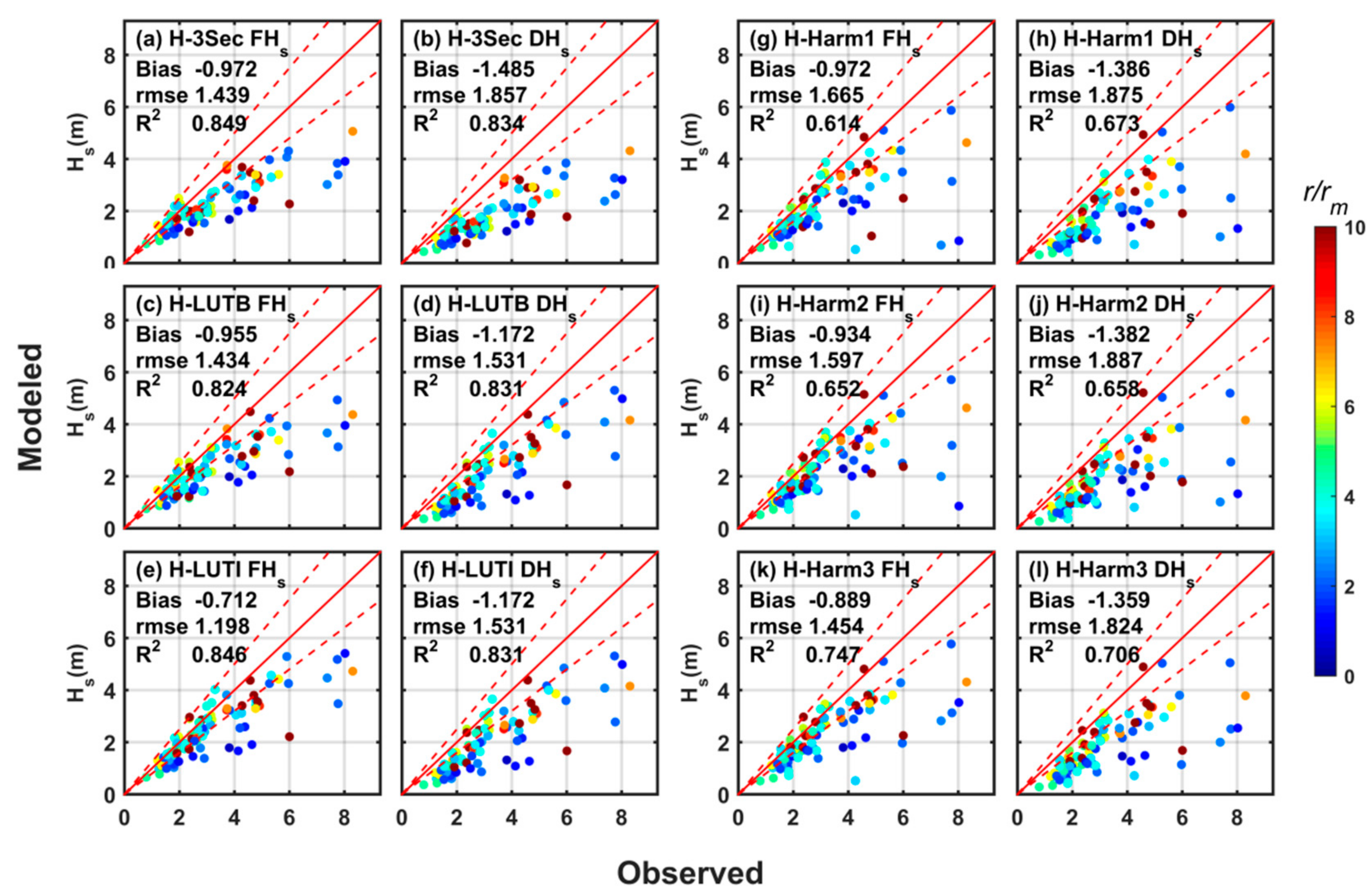
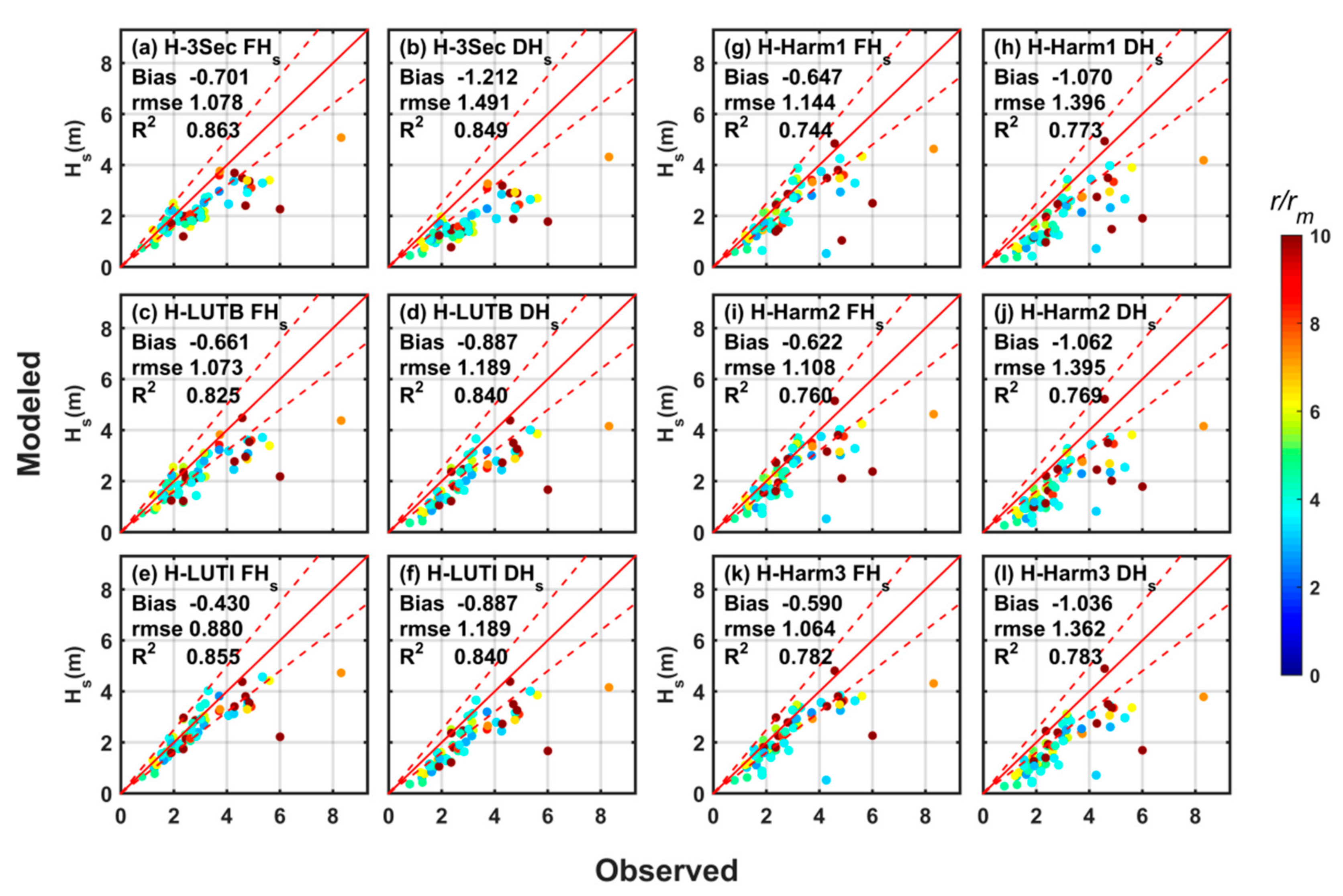
From July 2015 to December 2016, S1A acquired 86 SAR wave modes from 12 typhoons in the Northwest Pacific. Those SAR images are located less than 400 km from the typhoon center. For our selection condition, the maximum wind speed of the typhoon is relaxed to 20 m/s, including some conditions related to measurements in the generation and decay stages of the typhoon. Comparing the H-model simulation results to significant wave heights estimated by S1A, the scatter plots for wave heights (Figure 3) show that the models underestimate Hs to various extents, depending on the specific model; the deviations for results from DHs are generally greater than those from FHs.
The deviation of Hs from H-3Sec appears to be the most significant, especially for DHs. The root mean square error (rmse) reaches to 1.86 m. The models in the H-LUT group have a much finer resolution in the azimuthal direction and therefore better represent the surface wave development inside the typhoon than the H-3Sec model. Essentially, the results from H-LUTI model using the fetch-limited function have a bias of −0.71 m and rmse of 1.20 m, which are better than results from H-LUTB model. The H-Harm model group doesn’t perform very well in terms of the simulation error, though it is the only group of models that consider the impact of the radius of maximum wind speed. By increasing the number of components N in the Fourier series in Equation (9), the deviation and root mean square error of the associated models are reduced slightly. The model with N = 3, namely H-Harm3 appears to have the best performance among this group of models, corresponding to a deviation and rmse of −0.89 m and 1.45 m, respectively.
With respect to the correlation coefficient (R2) for the model results, H-3Sec and the H-LUT group have similar performances, with high values for R2 (about 0.84). They demonstrate that these models can simulate the Hs spatial distribution inside the typhoon well. The third set of models, H-Harm, has relatively poor correlation coefficients (average, 0.68). H-Harm3 is the best among this group with a correlation coefficient of 0.75 for FHs, and 0.71 for DHs. Therefore, based on this analysis, the H-LUTI model (with fetch) produces the most reliable spatial distribution of Hs, for a given wind speed, and has the least bias among these models.
Figure 3 compares estimates of Hs, as modeled by the H-models, with respect to measurements from S1A. The color bar represents the normalized radial distance r/rm from the typhoon center. Higher values of r/rm represent greater distance from the center of the typhoon. All model results show similar characteristics, namely that simulations close to the center of the typhoon have greater deviation from the Hs, compared to locations farther from the typhoon center. Taking the results from FHs of the H-LUTI model as an example, the spatial distribution of simulation errors in waves generated by typhoons is further discussed below.
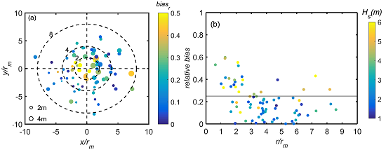
The relative deviations of wave height biasr = |Hs − FHs|/Hs for the H-LUTI model are shown, with the typhoon reference frame in Figure 4a. Overall, the simulated FHs values by H-LUTI model are in good agreement with significant wave heights from S1A. However, the relative deviation of the model is larger near the typhoon center and our results are in good agreement with those of Hwang et al. [42,43,44]. They suggested that these deviations may result from the presence of swell contamination, which may also be complicated by the processes in the typhoon centers and not resolved by relatively simple models. The biasr values are shown as a function of normalized radial distance in Figure 4b. The H-LUTI model has maximum relative deviation (about 60%) near the radius of maximum wind speed. Moreover, biasr constantly decreases with increasing normalized radial distance, until r/rm is more than 2.5, when the biasr is kept within about 25%.
Without including the area near the typhoon center, where r/rm is less than 2.5, the deviation and rmse for FHs simulated by H-LUTI model are reduced to −0.43 m and 0.88 m, respectively. The corresponding correlation coefficient reaches 0.86. Moreover, other H-models also are significantly improved, as shown in Figure 5.
In summary, other than the area near the typhoon center, significant wave heights can be estimated well by using the H-models, driven by of SAR-derived wind speed data. Of all the models, the best one is H-LUTI, which agrees well with the wave heights obtained from S1A measurements.
3.2. Wind Waves from RADARSAT-2 ScanSAR Mode Hurricane Winds
3.2.1. Validation by Wave Buoys
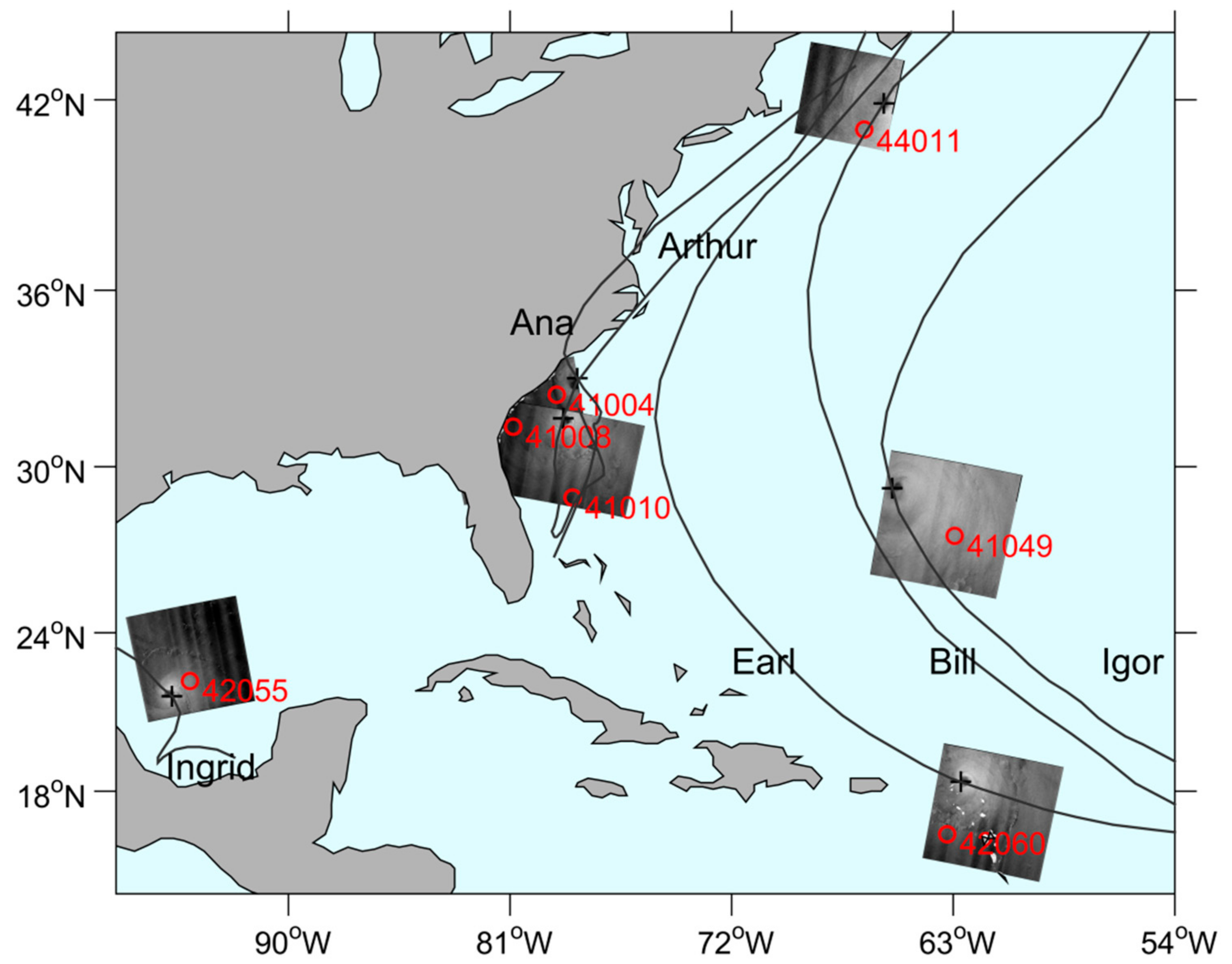
We collected 6 RADARSAT-2 cross-polarization (VH) SAR images covering six hurricanes acquired during the 2007–2017, collocated with 7 National Data Buoy Center (NDBC) buoys in the Gulf of Mexico and northwest Atlantic. The 6 SAR images include the centers of these hurricanes, as shown in Figure 6. Thus, these ScanSAR mode images capture part or the entire hurricane core, not as the wave mode images discussed above which only captured a small-range measurement of the hurricane. The best track data of the hurricanes was provided by NOAA, by the Extended Best Track Dataset. For each hurricane, SAR measurements are required to be within a 30-min window. Since a hurricane continues to move and rotate during this time window, we define the location of hurricane center by interpolation of the time series. A summary of the information for these hurricanes, including the locations of the hurricane center, maximum wind speeds and their radii, is given in Table 1. By using the C-2POD model, we directly obtained the wind speeds from these images, as shown in Figure 7.
The red circles in Figure 6 and Figure 7 show the locations of the buoys. A total of 7 buoys collected hourly wind speed and the wave spectra. Because H-models only apply to the wind waves, the wind waves are separated from wave spectra S(f) by the wave steepness method [54] developed by NDBC, in order to validate the models with buoy data. The significant wave heights of the wind sea are used to validate the H-models’ results, where is the upper frequency limit for wave spectra measurements and is the estimated separation frequency. All buoy wind speeds measured at different heights were adjusted to a reference level 10 m following [55]. To match the observation time of SAR images and buoys, the wave parameters and wind speeds are averaged over hourly intervals.
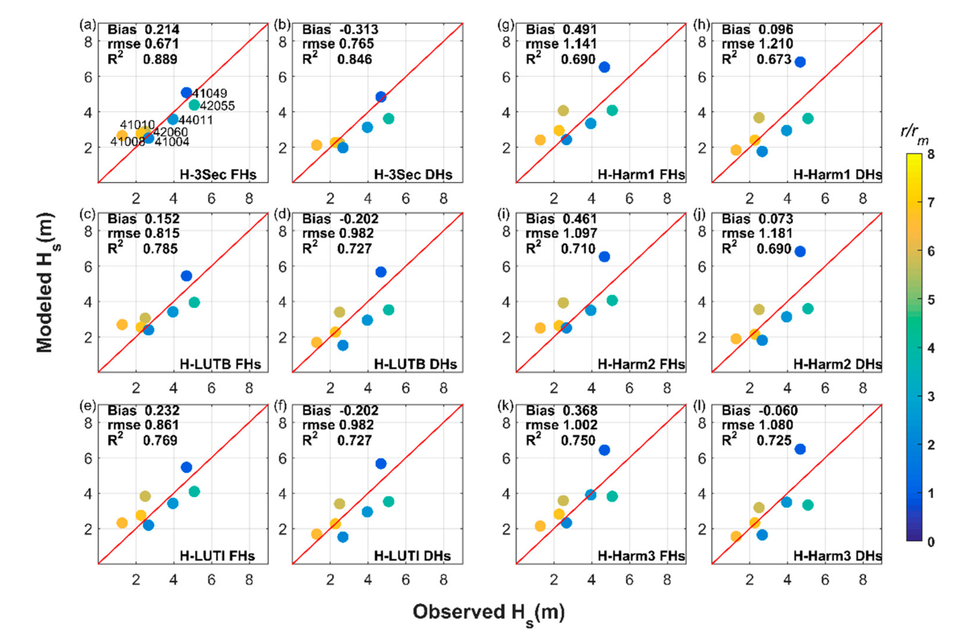
The C-2POD model is utilized to retrieve the hurricane wind fields from the SAR images, which also shows good agreement with the buoy wind measurements in this study (Figure 7g). Using the retrieved wind, the wave height and peak period can be estimated by 6 H-models with fetch- and duration- limited growth functions. Figure 8 presents the wave height comparisons between buoy measurements and retrievals from these SAR winds. The comparison with buoy wave heights supports some conclusions from the wave mode analysis. The computed wave heights using the fetch models are more accurate than those using the duration models, with smaller rmse and greater R2. The duration computations contain more underestimates, causing a negative bias in many H-models. Moreover, the H-3Sec model and the set of H-LUT models are considerably better than H-Harm models (rmse values of 0.67 m to 0.98 m vs. 1.00 m to 1.21 m; correlation coefficients of 0.73 to 0.89 vs. 0.67 to 0.75). The H-LUTI model using the fetch-limited function has rmse of 0.86 m and R2 of 0.77 here. It is also found that H-Harm3 with a higher value of N in the Fourier series (9) does the best simulation among the H-Harm models, whose rmse is 1.00 m and R2 is 0.75 for the fetch model result.
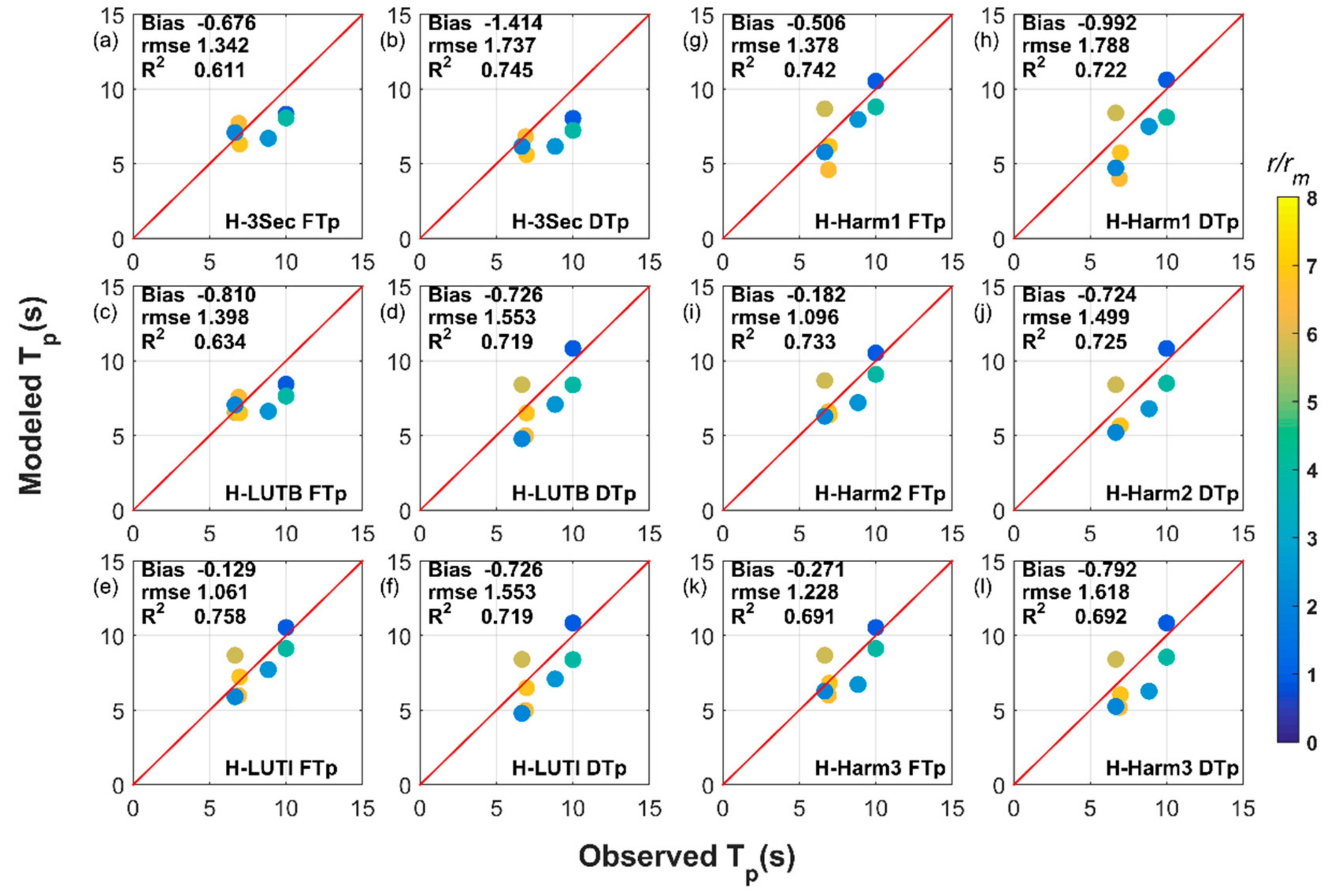
In Figure 9, the retrieved Tp is compared with buoy data. The negative bias for each of the H-models implies a tendency of those models to slightly underestimate the wave period. Similar to the results for the wave heights, the fetch models have better behavior in simulating Tp than the duration models, with rmse of 1.06 s to 1.40 s. The simulated FTp of H-LUTI model has the least rmse of 1.06 s and the highest R2 of 0.76 among the 6 H-models, which illustrates that the H-LUTI model is effective to simulate the dominant wave periods using the fetch-limited function. The wavelengths can be estimated from the dominant wave periods (approximately from 6 s to 10 s) according to the dispersion relationship, taking the water depths of the buoys into account. Thus, wind waves corresponding to 6 s~10 s, with wavelengths less than 150 m, can be retrieved, although they cannot be imaged directly by SAR because of the limited spatial resolution [24] and because of the cutoff caused by velocity bunching [14,15], especially in high sea states typical of tropical storms (e.g., larger than 450 m) [23]. The good agreement with buoy measurements is encouraging and indicates the possibilities for H-models to calculate dominant wave periods under hurricane conditions.
Since buoys tend to have reduced observational capabilities when the wind speeds approach hurricane force conditions, there were few buoys that were able to still function and to be captured in SRA images when hurricanes pass. Although buoys used to validate the H-models are quite limited, the results for the H-models robustly agree well with the buoy measurements. Therefore, H-models can potentially be used to retrieve the wave heights and peak periods from winds retrieved from RADARSAT-2 ScanSAR images, for example with application of the C-2POD model, taking advantage of cross-polarization SAR with its good sensitivity to higher wind speeds.
3.2.2. 2-Dimensional Application
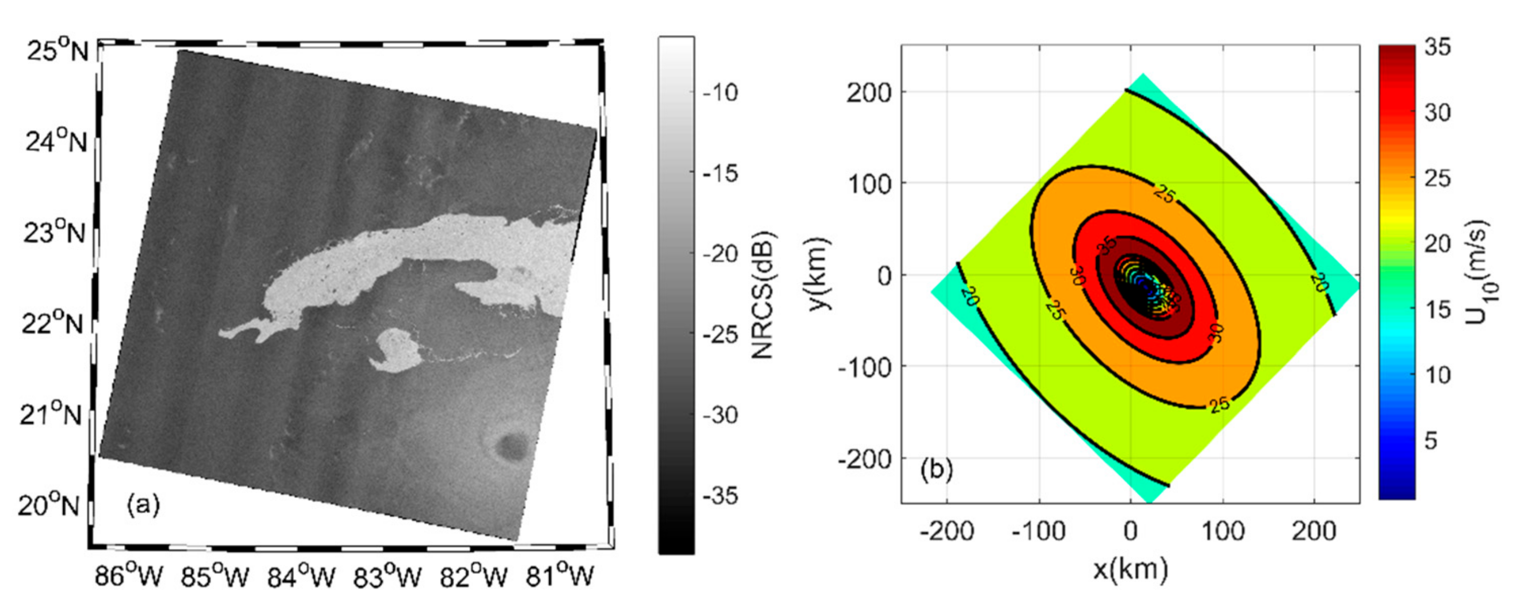
Figure 10a shows a RADARSAT-2 SAR image (only VH-channel image) acquired in ScanSAR mode with a 500 km swath for hurricane Gustav (2008). On basis of the VH-polarization SAR image, we can generate a wind map (Figure 10b) using a newly developed wind-retrieval algorithm, Symmetric Hurricane Estimates for Wind (SHEW) model [49]. The 2D hurricane winds are plotted, with the hurricane heading direction pointing toward the top of the page (unit: km). We only show the main area controlled by the hurricane, with the wind field calculated according to the symmetry of hurricane.
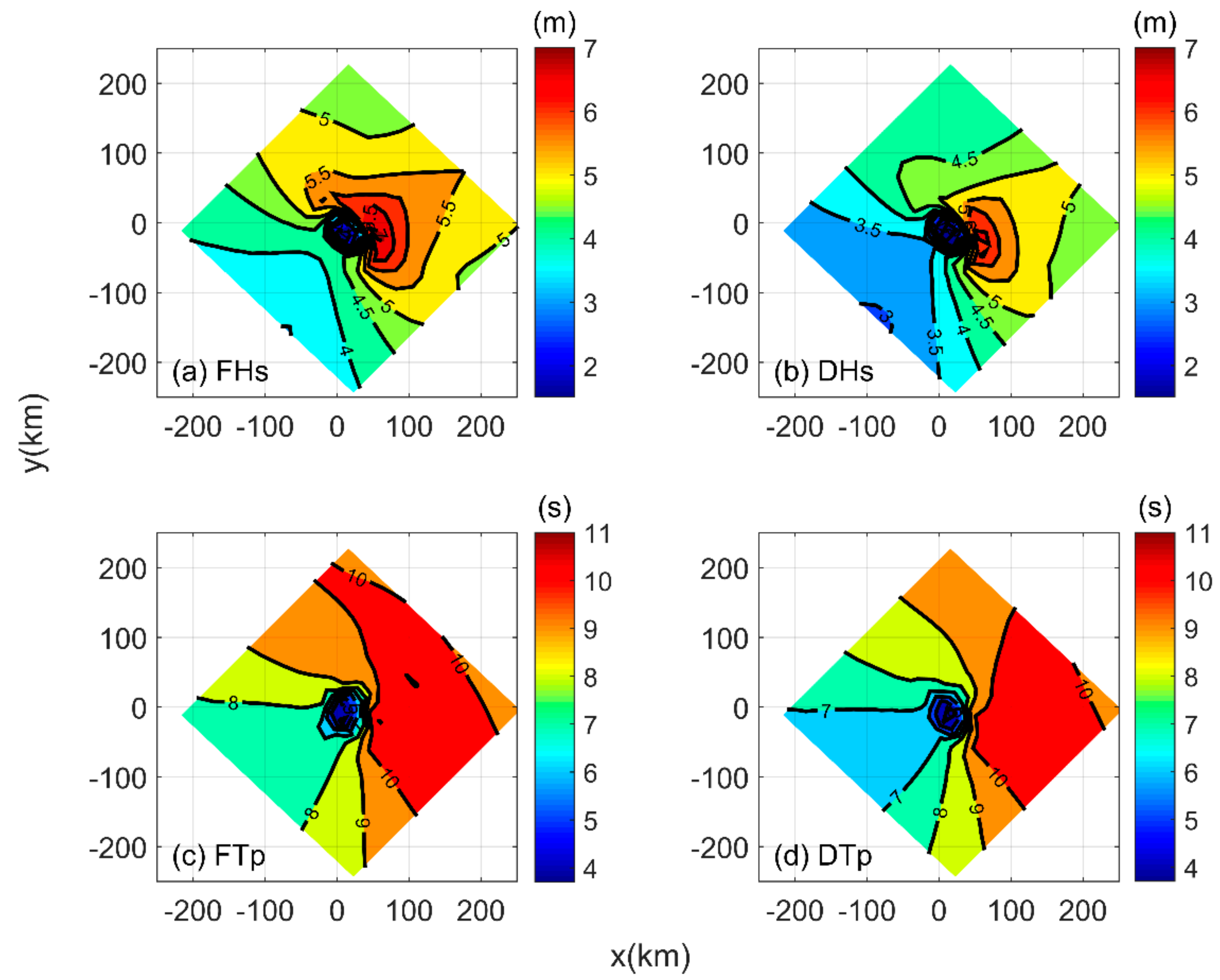
By using the H-LUTI model with the SAR-derived hurricane wind field, the significant wave heights and wave periods can be estimated (Figure 11). The results show that the location of maximum wave heights is within the right front regions, which is consistent with the previous studies of Young [56]. Since the wind vectors tend to be approximately aligned with the direction of propagation of the hurricane, waves generated in this area tend to move forward with the hurricane and hence remain in the intense wind regions for extended period of time (extended fetch), conversely, to the left of the hurricane center. As a result, the spatial distribution of the wave field is not exactly symmetric.
The simulation of Tp is shown in Figure 11c,d. Although the simulation results from the H-LUTI model can describe the wave distribution features well for the longer wave periods on the right front side of the hurricane, the accuracy of the results still needs to be verified in additional studies with more buoy measurements.
4. Discussion
All of the models are based on the implicit initial assumption regarding the essential role of nonlinear wave-wave interactions in maintaining the wave spectrum similarity. Moreover, many studies have shown that most of the spectra are monomodal under extreme conditions, similar to the spectra generated under fetch-limited, steady wind conditions. However, bi-modal spectra are also found in both measurements and model results under intense cyclone conditions [11,29,31], in which case the accuracy of the parametric models used in this study can be degraded. For instance, this is the case in the cyclone’s left forward quadrant where the direction of wind deviates considerably from the wave direction [31]. As shown in a previous study [11], the analysis of directional spectra observed by Extreme Air-Sea Interaction buoys shows that a variety of spectral geometries can exist close to the eyes of typhoons. Thus, the effectiveness of the simple fetch-limited parametric models should be further discussed, in terms of the cyclone quadrant under consideration, and the rate of development or change the intensity of the storm.
In this context, we suggest that the H-LUTI model is the best among the three H-models. Regarding the original studies that developed the H-models, it is not difficult to infer the reasons for this result. Firstly, the H-LUT models simulate wind wave parameters along comparatively more transects radiating from the storm center, improving on the H-3Sec model’s ability to simulate the development of the azimuthal and radial variations of the surface waves. Moreover, as shown in Figure 1 of [44], the dataset from Ivan (2014) used to develop the H-LUTI model contains more observational transects inside the storm coverage region than the dataset from Bonnie (1998) used in development of the H-LUTB model, thus providing a better azimuthal resolution for fitting the empirical model. Many previous studies [39,40,41,56] clearly demonstrate that the equivalent fetch and duration of storm is associated with the relative position of the storm, the velocity of forward movement of the storm, maximum wind speed and the radius of maximum wind speed. However, for the third set of models, the H-Harm models, a systematic quasi-linear variation of the harmonic parameters and with the radius of maximum wind rm (Equation (10)) was established based on only 4 storm datasets. These 4 datasets have different values for rm, which have only a limited coverage range, leading to their relatively poor performance. Therefore, in future studies, it is particularly important to collect a large number of simultaneous wind and wave measurements under conditions appropriate for these storms in order to optimize the wave model.
5. Conclusions
Making use of the fetch- or duration-limited H-models, the basic typhoon/hurricane wind wave parameters can be estimated by only using the SAR-derived wind field data. This approach provides a new method for detecting typhoon/hurricane wind waves from SAR measurements. We show that the H-models can effectively calculate the significant wave heights inside the typhoon based on wind observations from Sentinel-1A (S1A) SAR images, except in the area near the typhoon center. Comparing the results with wave heights measured by S1A, we show that the wave heights calculated from the fetch-limited function (FHs) are always larger than those calculated by the duration-limited function (DHs), and in good agreement with the S1A wave height estimates. Among the results of these three set of H-models, the best one is the H-LUTI model using the fetch-limited function, which has a root mean square error of 0.88 m, and correlation coefficient of 0.86. Operating in ScanSAR mode, the H-models also have the potential to reliably simulate Hs and Tp for wind waves inside hurricanes from RADARSAT-2 ScanSAR mode observations, based on similar statistical properties derived from verifications by buoy data. The H-LUTI model is especially notable with results using the fetch function that are good, with rmse of 0.86 m and R2 of 0.77 for Hs, and rmse of 1.06 s and R2 of 0.76 for Tp. Furthermore, this model works well to describe the high values of significant wave heights and dominant wave periods in the right frontal regions of the typhoons/hurricanes.
Author Contributions
G.L. contributed to the idea of this study and suggested for the topic; L.Z. collected and analyzed the data; L.Z. wrote the original draft; G.Z. helped a lot to prepare the wind finds; G.L., W.P. and Y.H. assisted in manuscript preparation and revision.
Funding
This research was funded by the National Key Research and Development Program of China 2016YFC1401407; National Natural Science Foundation of China under Grant 41506028; Natural Science Foundation of Jiangsu Province under Grant BK20150913; the Startup Foundation for Introducing Talent of NUIST; the International cooperation project of National Natural Science Foundation of China under Grant 41620104003; National Program on Global Change and Air-Sea Interaction under Grant GASI-IPOVAI-04; the Office of Energy Research and Development (OERD) project 1B00.003C; the Canadian Space Agency Data Utilization and Applications Program (DUAP) project 14SURM006; MEOPAR (Marine Environmental Observation Prediction and Response Network) project 1P1.2 and in part by National Natural Science Youth Foundation of China under Grant 41706193.
Acknowledgments
We thank Paul Hwang for sharing the fetch- and duration-limited parametric models’ codes at https://www.researchgate.net/publication/ 315772258_HurricaneFetchDurPackage.
Conflicts of Interest
The authors declare no conflict of interest.
References
- Craig, P.D.; Banner, M.L. Modeling wave-enhanced turbulence in the ocean surface layer. J. Phys. Oceanogr. 1994, 24, 2546–2559. [Google Scholar] [CrossRef]
- Craig, P.D. Velocity profiles and surface roughness under breaking waves. J. Geophys. Res. 1996, 101, 1265–1277. [Google Scholar] [CrossRef]
- Toffoli, A.; McConochie, J.; Ghantous, M.; Loffredo, L.; Babanin, A.V. The effect of wave-induced turbulence on the ocean mixed layer during tropical cyclones: Field observations on the Australian North-West Shelf. J. Geophys. Res. 2012, 117, 1–8. [Google Scholar] [CrossRef]
- Reichl, B.G.; Wang, D.; Hara, T.; Ginis, I.; Kukulka, T. Langmuir turbulence parameterization in tropical cyclone conditions. J. Phys. Oceanogr. 2016, 46, 863–886. [Google Scholar] [CrossRef]
- Perrie, W.; Toulany, B.; Roland, A.; Dutour-Sikiric, M.; Chen, C.; Beardsley, R.C.; Chen, C.; Beardsley, R.C.; Qi, J.; Hu, Y.; et al. Modeling North Atlantic Nor’easters with modern wave forecast models. J. Geophys. Res. 2018, 123, 533–557. [Google Scholar] [CrossRef]
- Cardone, V.J.; Jensen, R.E.; Resio, D.T.; Swail, V.R.; Cox, A.T. Evaluation of contemporary ocean wave models in rare extreme events: The Halloween Storm of October 1991 and the Stormof the Century of March 1993. J. Atmos. Ocean. Technol. 1996, 13, 198–230. [Google Scholar] [CrossRef]
- Beal, R.C.; Gerling, T.W.; Irvine, D.E.; Monaldo, F.M. Spatial variations of ocean wave directional spectra from the Seasat synthetic aperture radar. J. Geophys. Res. 1986, 91, 2433–2449. [Google Scholar] [CrossRef]
- Wright, C.W.; Walsh, E.J.; Vandemark, D.; Krabill, W.B.; Garcia, A.W.; Houston, S.H.; Powell, M.D.; Black, P.G.; Marks, F.D. Hurricane directional wave spectrum spatial variation in the open ocean. J. Phys. Oceanogr. 2001, 31, 2472–2488. [Google Scholar] [CrossRef]
- Walsh, E.J.; Wright, C.W.; Vandemark, D.; Krabill, W.B.; Garcia, A.W.; Houston, S.H.; Murillo, S.T.; Powell, M.D.; Black, P.G.; Marks, F.D., Jr. Hurricane directional wave spectrum spatial variation at landfall. J. Phys. Oceanogr. 2002, 32, 1667–1684. [Google Scholar] [CrossRef]
- Forristall, G.Z.; Ward, E.G.; Cardone, V.J.; Borgmann, L.E. The directional spectra and kinematics of surface gravity waves in tropical storm Delia. J. Phys. Oceanogr. 1978, 8, 888–909. [Google Scholar] [CrossRef]
- Collins, C.O.; Potter, H.; Lund, B.; Tamura, H.; Graber, H.C. Directional wave spectra observed during intense tropical cyclones. J. Geophys. Res. 2018, 123, 773–793. [Google Scholar] [CrossRef]
- Collins, C.O. Typhoon Generated Surface Gravity Waves Measured by NOMAD-Type Buoys. Ph.D. Thesis, University of Miami, Coral Gables, FL, USA, 2014. [Google Scholar]
- Xu, Y.; He, H.; Song, J.; Hou, Y.; Li, F. Observations and Modeling of Typhoon Waves in the South China Sea. J. Phys. Oceanogr. 2017, 47, 1307–1324. [Google Scholar] [CrossRef]
- Hasselmann, K.; Hasselmann, S. On the nonlinear mapping of an ocean wave spectrum into a synthetic aperture radar image spectrum and its inversion. J. Geophys. Res. 1991, 96, 10713–10729. [Google Scholar] [CrossRef]
- Mastenbroek, C.D.; Valk, C.D. A semiparametric algorithm to retrieve ocean wave spectra from synthetic aperture radar. J. Geophys. Res. 2000, 105, 3497–3516. [Google Scholar] [CrossRef] [Green Version]
- Sun, J.; Guan, C.L. Parameterized first-guess spectrum method for retrieving directional spectrum of swell-dominated waves and huge waves from SAR images. Chin. J. Oceanol. Limnol. 2006, 24, 12–20. [Google Scholar]
- Sun, J.; Kawamura, H. Retrieval of surface wave parameters from SAR images and their validation in the coastal seas around Japan. J. Oceanogr. 2009, 65, 567–577. [Google Scholar] [CrossRef]
- Shao, J.; Li, X.; Sun, J. Ocean wave parameters retrieval from TerraSAR-X images validated against buoy measurements and model results. Remote Sens. 2015, 7, 12815–12828. [Google Scholar] [CrossRef]
- Schulz-Stellenfleth, J.; Lehner, S.; Hoja, D. A parametric scheme for the retrieval of two-dimensional ocean wave spectra from synthetic aperture radar look cross spectra. J. Geophys. Res. 2005, 110, 297–314. [Google Scholar] [CrossRef]
- Hasselmann, K.; Raney, R.K.; Plant, W.J.; Alpers, W.; Shuchman, R.A.; Lyzenga, D.R.; Rufenach, C.L.; Tucker, M.J. Theory of synthetic aperture radar ocean imaging: A MARSEN view. J. Geophys. Res. 2005, 90, 4659–4686. [Google Scholar] [CrossRef]
- Schulz-Stellenfleth, J.; König, T.; Lehner, S. An empirical approach for the retrieval of integral ocean wave parameters from synthetic aperture radar data. J. Geophys. Res. 2007, 112, 1–14. [Google Scholar] [CrossRef]
- Li, X.; Lehner, S.; Bruns, T. Ocean wave integral parameter measurements using Envisat ASAR wave mode data. IEEE Trans. Geosci. Remote Sens. 2011, 49, 155–174. [Google Scholar] [CrossRef] [Green Version]
- Stopa, J.E.; Mouche, A. Significant wave heights from Sentinel-1 SAR: Validation and applications. J. Geophys. Res. 2017, 122, 1827–1848. [Google Scholar] [CrossRef]
- Romeiser, R.; Graber, H.C.; Caruso, M.J.; Jensen, R.E.; Walker, D.T.; Cox, A.T. A new approach to ocean wave parameter estimates from C-band ScanSAR images. IEEE Trans. Geosci. Remote Sens. 2015, 53, 1320–1345. [Google Scholar] [CrossRef]
- Zhang, B.; Li, X.; Perrie, W.; He, Y. Synergistic measurements of ocean winds and waves from SAR. J. Geophys. Res. 2015, 120, 6164–6184. [Google Scholar] [CrossRef]
- Zhang, B.; Perrie, W.; He, Y. Validation of RADARSAT-2 fully polarimetric SAR measurements of ocean surface waves. J. Geophys. Res. 2010, 115, 1–11. [Google Scholar] [CrossRef]
- Xie, T.; Perrie, W.; He, Y.; Li, H.; Fang, H.; Zhao, S.; Yu, W. Ocean surface wave measurements from fully polarimetric SAR imagery. Sci. China Earth Sci. 2015, 58, 1849–1861. [Google Scholar] [CrossRef]
- Young, I.R. Observations of the spectra of hurricane generated waves. Ocean Eng. 1998, 25, 361–376. [Google Scholar] [CrossRef]
- Young, I.R. Directional spectra of hurricane wind waves. J. Geophys. Res. 2006, 111, 1–14. [Google Scholar] [CrossRef]
- Ochi, M.K. Hurricane-Generated Seas; Elsevier: Oxford, UK, 2003; pp. 25–53. [Google Scholar]
- Hu, K.; Chen, Q. Directional spectra of hurricane-generated waves in the Gulf of Mexico. Geophys. Res. Lett. 2011, 38, 1–7. [Google Scholar] [CrossRef]
- Kudryavtsev, V.; Golubkin, P.; Chapron, B. A simplified wave enhancement criterion for moving extreme events. J. Geophys. Res-Oceans 2016, 120, 7538–7558. [Google Scholar] [CrossRef]
- Badulin, S.I.; Pushkarev, A.N.; Resio, D.; Zakharov, V.E. Self-similarity of wind-driven seas. Nonlinear Proc. Geoph. 2005, 12, 891–945. [Google Scholar] [CrossRef] [Green Version]
- Zakharov, V.E. Theoretical interpretation of fetch limited wind-drivensea observations. Nonlinear Proc. Geoph. 2005, 12, 1011–1020. [Google Scholar] [CrossRef] [Green Version]
- Resio, D.; Perrie, W. A numerical study of nonlinear energy fluxes due to wave-wave interactions Part 1. Methodology and basic results. J. Fluid Mech. 1991, 223, 603–629. [Google Scholar] [CrossRef]
- Resio, D.; Long, C.; Perrie, W. The effect of nonlinear fluxes on spectral shape and energy source-sink balances in wave generation. J. Phys. Oceanogr. 2011, 41, 781–801. [Google Scholar] [CrossRef]
- Banner, M.L.; Young, I.R. Modeling spectral dissipation in the evolution of wind waves. Part 1. Assessment of existing model performance. J. Phys. Oceanogr. 1994, 24, 1550–1671. [Google Scholar] [CrossRef]
- The SWAMP Group. Sea Wave Modelling Project (SWAMP). An Intercomparison Study of Wind Wave Prediction Models. Part 1: Principal Results and Conclusions; Ocean Wave Modeling; Plenum Press: New York, NY, USA, 1985. [Google Scholar]
- Young, I.R. Parametric hurricane wave prediction model. J. Waterw. Port Coast. Ocean Eng. 1988, 114, 637–652. [Google Scholar] [CrossRef]
- Young, I.R.; Burchell, G.P. Hurricane generated waves as observed by satellite. Ocean Eng. 1996, 23, 761–776. [Google Scholar] [CrossRef]
- Young, I.R.; Vinoth, J. An “extended fetch” model for the spatial distribution of tropical cyclone wind–waves as observed by altimeter. Ocean Eng. 2013, 70, 14–24. [Google Scholar] [CrossRef]
- Hwang, P. Fetch-and duration-limited nature of surface wave growth inside tropical cyclones: With applications to air–sea exchange and remote sensing. J. Phys. Oceanogr. 2016, 46, 41–56. [Google Scholar] [CrossRef]
- Hwang, P.; Walsh, E.J. Azimuthal and radial variation of wind-generated surface waves inside tropical cyclones. J. Phys. Oceanogr. 2016, 46, 2605–2621. [Google Scholar] [CrossRef]
- Hwang, P.; Fan, Y. Effective fetch and duration of tropical cyclone wind fields estimated from simultaneous wind and wave measurements: Surface wave and air–sea exchange computation. J. Phys. Oceanogr. 2017, 47, 447–470. [Google Scholar] [CrossRef]
- Zhang, B.; Perrie, W. Cross-polarized synthetic aperture radar: A new potential measurement technique for hurricanes. Bull. Am. Meteorol. Soc. 2012, 93, 531–541. [Google Scholar] [CrossRef]
- Zhang, B.; Perrie, W.; Zhang, J.A.; Uhlhorn, E.W.; He, Y. High-resolution hurricane vector winds from C-band dual-polarization SAR observations. J. Atmos. Ocean. Technol. 2014, 31, 272–286. [Google Scholar] [CrossRef]
- Horstmann, J.; Wackerman, C.; Falchetti, S.; Maresca, S. Tropical cyclone winds retrieved from synthetic aperture radar. Oceanography 2013, 26, 46–57. [Google Scholar] [CrossRef]
- Van Zadelhoff, G.-J.; Stoffelen, A.; Vachon, P.W.; Wolfe, J.; Horstmann, J.; Belmonte Rivas, M. Retrieving hurricane wind speeds using cross-polarization C-band measurements. Atmos. Meas. Tech. 2014, 7, 437–449. [Google Scholar] [CrossRef] [Green Version]
- Zhang, G.; Perrie, W.; Li, X.; Zhang, J.A. A hurricane morphology and sea surface wind vector estimation model based on C-band cross-polarization SAR imagery. IEEE Trans. Geosci. Remote Sens. 2017, 55, 1743–1751. [Google Scholar] [CrossRef]
- Zhang, G.; Li, X.; Perrie, W.; Hwang, P.A.; Zhang, B.; Yang, X. A Hurricane wind speed retrieval model for C-band RADARSAT-2 cross-polarization ScanSAR images. IEEE Trans. Geosci. Remote Sens. 2017, 55, 4766–4774. [Google Scholar] [CrossRef]
- Mouche, A.A.; Chapron, B.; Zhang, B.; Husson, R. Combined co- and cross-polarized SAR measurements under extreme wind conditions. IEEE Trans. Geosci. Remote Sens. 2017, 55, 6746–6755. [Google Scholar] [CrossRef]
- Engen, G.; Johnsen, H. SAR-ocean wave inversion using image cross spectra. IEEE Trans. Geosci. Remote Sens. 1995, 33, 1047–1056. [Google Scholar] [CrossRef]
- Hwang, P.; Fan, Y.; Ocampo-Torres, F.J.; García-Nava, H. Ocean Surface Wave Spectra inside Tropical Cyclones. J. Phys. Oceanogr. 2017, 47, 2393–2417. [Google Scholar] [CrossRef]
- Gilhousen, D.B.; Hervey, R. Improved estimates of swell from moored buoys. Ocean Wave Meas. Anal. 2001, 2002, 387–393. [Google Scholar]
- Atlas, R.; Hoffman, R.N.; Ardizzone, J.; Leidner, S.M.; Jusem, J.C.; Smith, D.K.; Gombos, D. A cross-calibrated, multiplatform ocean surface wind velocity product for meteorological and oceanographic applications. Bull. Am. Meteorol. Soc. 2011, 92, 157–174. [Google Scholar] [CrossRef]
- Young, I.R. A Review of Parametric Descriptions of Tropical Cyclone Wind-Wave Generation. Atmosphere 2017, 8, 194. [Google Scholar] [CrossRef]
Figure 1.
(a) The best track for typhoon Krovanh. The maximum wind speed (m/s) is denoted by the color of circles. Red crosses represent the typhoon centers as S1A passed through. The colored squares represent the SAR wave mode images observed by S1A (1st pass: blue; 2nd pass: green; 3rd pass: red). (b) SAR wave mode images in the typhoon reference frame (colored squares). The corresponding radius of maximum wind speed is denoted by dashed line. In (b), the coordinates (x, y) are rotated such that the typhoon heading is toward the top of the page. The x and y present the left-right and front-back distances with respect to the typhoon center, respectively.
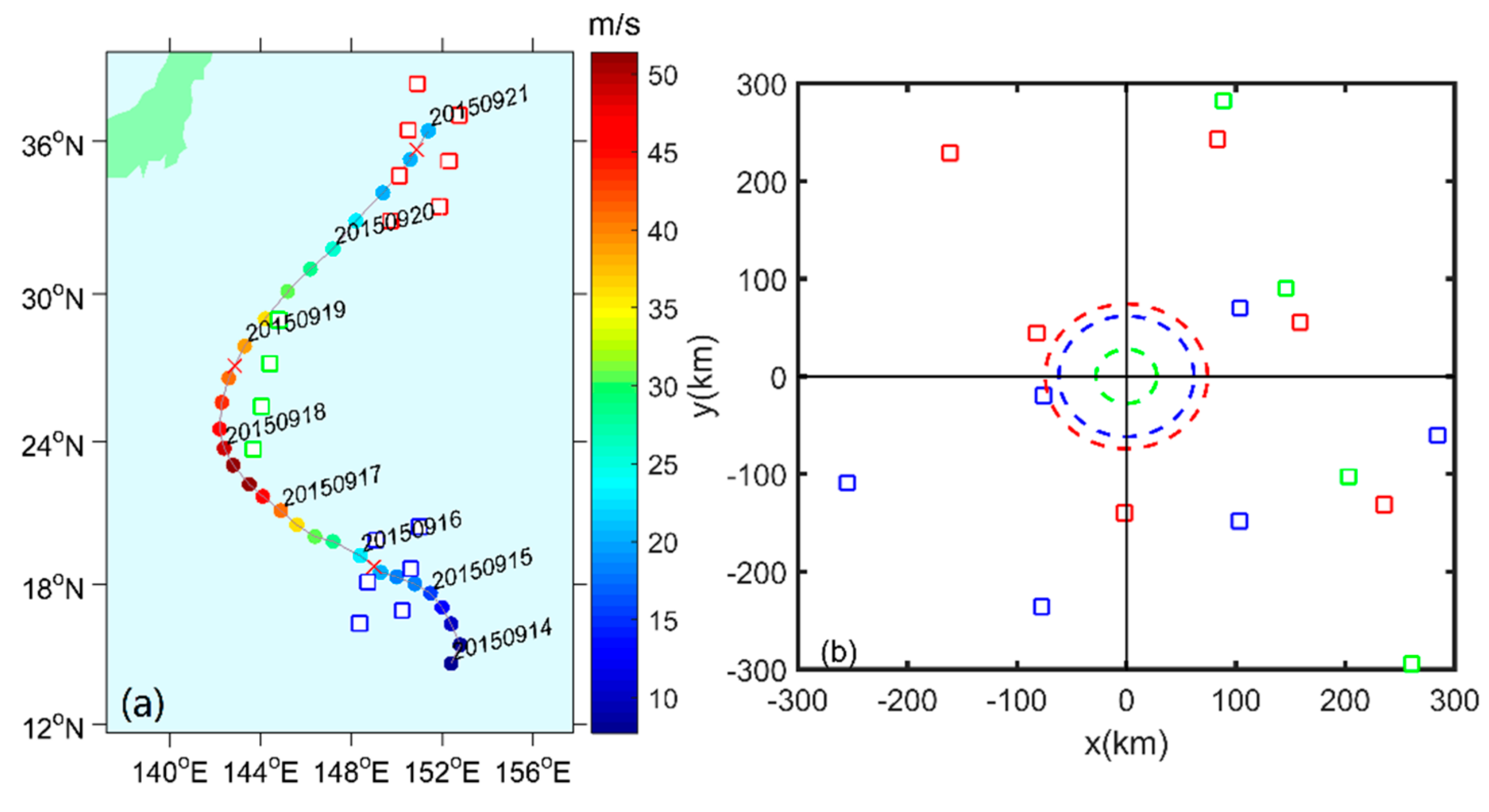
Figure 2.
Radial (a,c,e,g,i,k) and azimuthal (b,d,f,h,j,l) variations of Hs provided by S1A Level-2 products (colored squares) and modeled by H-models (FHs: magenta solid points; DHs: black solid points). The colors of the squares denote the sampling sequence (1st pass: blue; 2nd pass: Green; 3rd pass: red).

Figure 3.
Comparison of Hs provided by S1A measurements and modeled by H-models. The color represents the normalized distance from the typhoon center (r/rm). For reference, the red lines correspond to 1:1 (solid line) and 1:1.25 (1.25:1) (dashed lines).
Figure 3.
Comparison of Hs provided by S1A measurements and modeled by H-models. The color represents the normalized distance from the typhoon center (r/rm). For reference, the red lines correspond to 1:1 (solid line) and 1:1.25 (1.25:1) (dashed lines).

Figure 4.
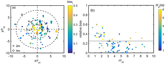
(a) The relative bias of FHs modeled by H-LUTI shown in the typhoon reference frame, with the typhoon center located at the center of the figure and the coordinates showing the distance to the typhoon center scaled by the radius of the maximum wind speed rm. The propagation direction of typhoon is toward the top of the page. The color and size of the solid circles correspond to biasr and Hs, respectively. The larger concentric dashed-line cycles indicate r/rm =2, 4 and 8. (b) the relative bias as the function of r/rm. The color denotes the values for Hs as measured by S1A. The solid line marks the biasr = 0.25.
Figure 4.
(a) The relative bias of FHs modeled by H-LUTI shown in the typhoon reference frame, with the typhoon center located at the center of the figure and the coordinates showing the distance to the typhoon center scaled by the radius of the maximum wind speed rm. The propagation direction of typhoon is toward the top of the page. The color and size of the solid circles correspond to biasr and Hs, respectively. The larger concentric dashed-line cycles indicate r/rm =2, 4 and 8. (b) the relative bias as the function of r/rm. The color denotes the values for Hs as measured by S1A. The solid line marks the biasr = 0.25.
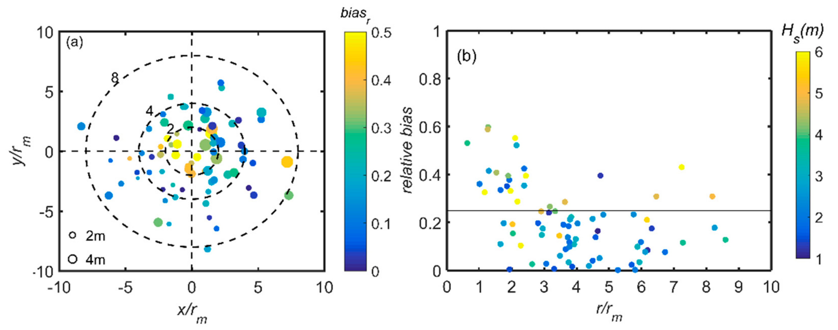
Figure 5.
As Figure 4 but for comparison of Hs provided by S1A measurements to modeled estimates provided by 6 H-models except near the eye region (r/rm < 2.5).
Figure 5.
As Figure 4 but for comparison of Hs provided by S1A measurements to modeled estimates provided by 6 H-models except near the eye region (r/rm < 2.5).

Figure 6.
The RADARSAT-2 ScanSAR images for selected hurricanes with the best track data set; the 7 buoys covered by SAR images are presented as red circles.
Figure 6.
The RADARSAT-2 ScanSAR images for selected hurricanes with the best track data set; the 7 buoys covered by SAR images are presented as red circles.

Figure 7.
(a–f) Hurricane wind speeds retrieved by C-2POD wind retrieval model for the 6 SAR images shown in Figure 6. The superimposed arrows show the hurricane heading direction with the root of the arrow at the hurricane center. The length of the arrows represents the velocity of forward movement of hurricanes: (a) 55.19 km/h (b) 23.40 km/h (c) 23.40 km/h (d) 11.85 km/h (e) 18.65 km/h (f) 9.25 km/h. (g) Comparisons of retrieved wind speeds with collected buoys measurements.
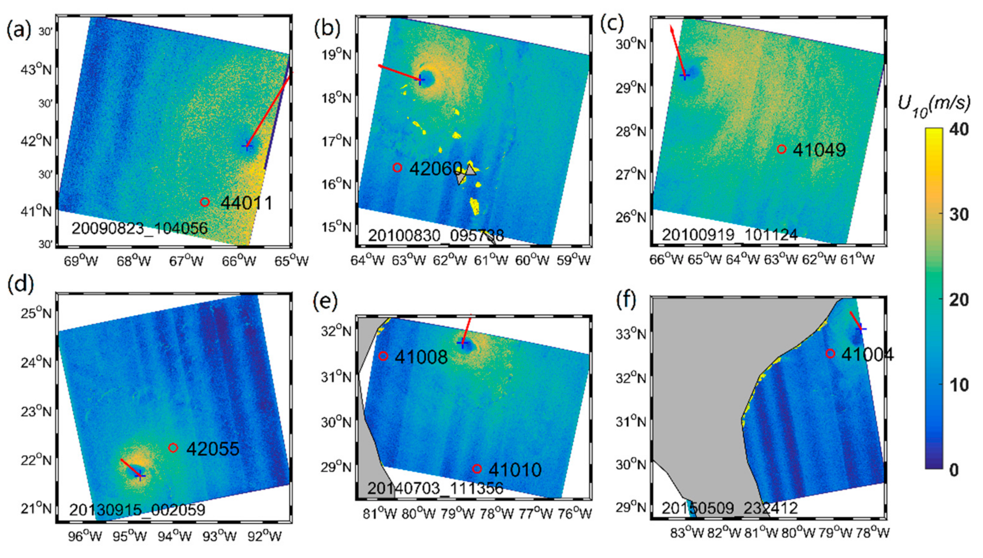
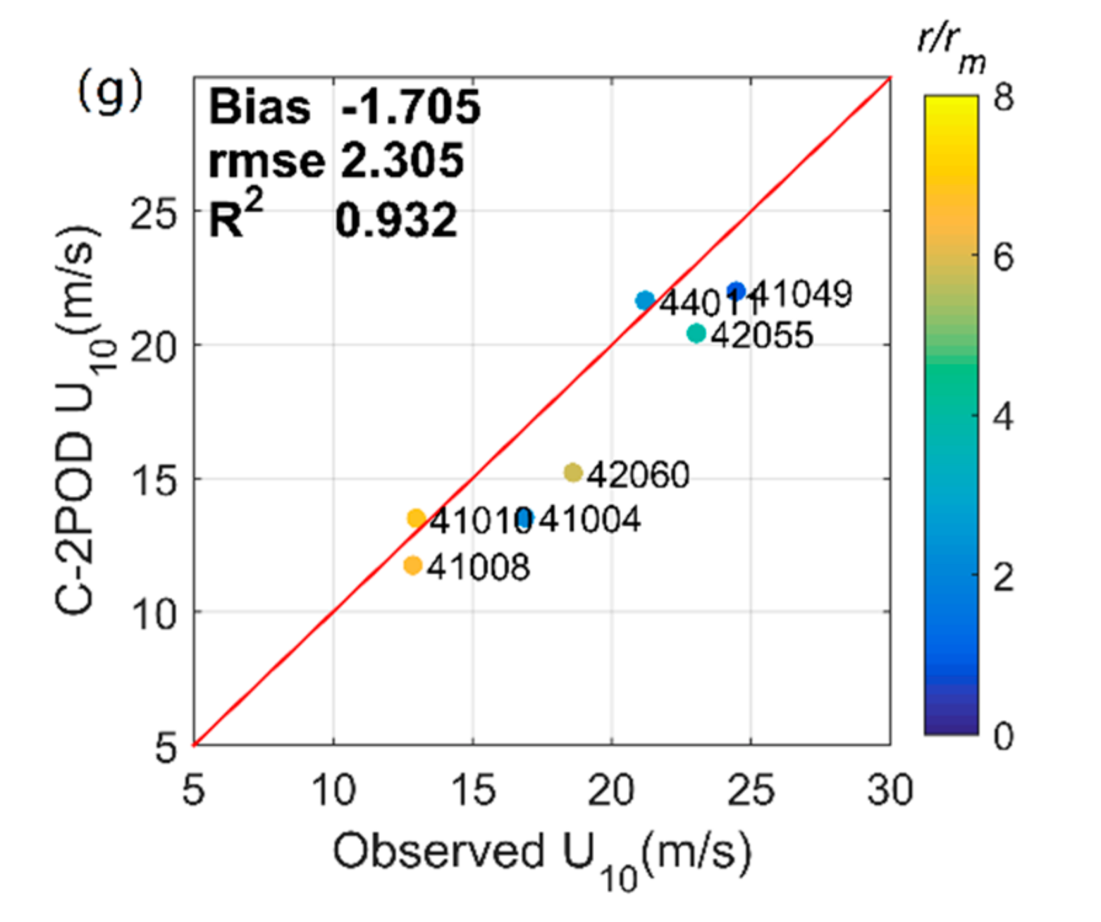
Figure 8.
Comparison of Hs retrieval from SAR-derived winds, using fetch- (a,c,e,g,i,k) or duration-limited (b,d,f,h,j,l) growth models, and the buoy observations. Results for 6 models are presented: H-3Sec, H-LUTB, H-LUTI, H-Harm1, H-Harm2, and H-Harm3.
Figure 8.
Comparison of Hs retrieval from SAR-derived winds, using fetch- (a,c,e,g,i,k) or duration-limited (b,d,f,h,j,l) growth models, and the buoy observations. Results for 6 models are presented: H-3Sec, H-LUTB, H-LUTI, H-Harm1, H-Harm2, and H-Harm3.

Figure 9.
Comparison of Tp retrieved from SAR-derived winds, using fetch- (a,c,e,g,i,k) or duration-limited (b,d,f,h,j,l) growth models, and the buoy observations. Results for 6 models are presented: H-3Sec, H-LUTB, H-LUTI, H-Harm1, H-Harm2, and H-Harm3.
Figure 9.
Comparison of Tp retrieved from SAR-derived winds, using fetch- (a,c,e,g,i,k) or duration-limited (b,d,f,h,j,l) growth models, and the buoy observations. Results for 6 models are presented: H-3Sec, H-LUTB, H-LUTI, H-Harm1, H-Harm2, and H-Harm3.

Figure 10.
(a) RADARSAT-2 ScanSAR image acquired over hurricane Gustav at 1128UTC 30 August 2008. (b) SAR-retrieved wind speed.
Figure 10.
(a) RADARSAT-2 ScanSAR image acquired over hurricane Gustav at 1128UTC 30 August 2008. (b) SAR-retrieved wind speed.

Figure 11.
(a) Wave height from fetch-limited growth function FHs, (b) wave height from duration-limited growth function DHs, (c) wave period from fetch-limited growth function FTp and (d) wave period from duration-limited growth function DTp modeled by H-LUTI.
Figure 11.
(a) Wave height from fetch-limited growth function FHs, (b) wave height from duration-limited growth function DHs, (c) wave period from fetch-limited growth function FTp and (d) wave period from duration-limited growth function DTp modeled by H-LUTI.


Table 1.
Basic information of hurricanes, Bill 2009, Earl 2010, Igor 2010, Ingrid 2013, Arthur 2014 and Ana 2015. The um and rm represent maximum wind speed and radius of maximum wind speed.
Table 1.
Basic information of hurricanes, Bill 2009, Earl 2010, Igor 2010, Ingrid 2013, Arthur 2014 and Ana 2015. The um and rm represent maximum wind speed and radius of maximum wind speed.
| Hurricane Names | Date (yyyy-mm-dd) | Time (UTC) | Center | um (m/s) | rm (km) | |
|---|---|---|---|---|---|---|
| Latitude | Longitude | |||||
| Bill | 2009-08-23 | 10:40:56 | 41.89°N | −65.82°E | 36.57 | 74.08 |
| Earl | 2010-08-30 | 09:57:38 | 18.36°N | −62.69°E | 52.26 | 49.45 |
| Igor | 2010-09-19 | 10:11:24 | 29.24°N | −65.48°E | 38.58 | 92.60 |
| Ingrid | 2013-09-15 | 00:20:59 | 21.62°N | −94.73°E | 38.58 | 37.04 |
| Arthur | 2014-07-03 | 11:13:56 | 31.68°N | −78.84°E | 40.49 | 39.41 |
| Ana | 2015-05-09 | 23:24:12 | 33.06°N | −78.27°E | 23.15 | 74.08 |
© 2018 by the authors. Licensee MDPI, Basel, Switzerland. This article is an open access article distributed under the terms and conditions of the Creative Commons Attribution (CC BY) license (http://creativecommons.org/licenses/by/4.0/).
Share and Cite
MDPI and ACS Style
Zhang, L.; Liu, G.; Perrie, W.; He, Y.; Zhang, G. Typhoon/Hurricane-Generated Wind Waves Inferred from SAR Imagery. Remote Sens. 2018, 10, 1605. https://doi.org/10.3390/rs10101605
AMA Style
Zhang L, Liu G, Perrie W, He Y, Zhang G. Typhoon/Hurricane-Generated Wind Waves Inferred from SAR Imagery. Remote Sensing. 2018; 10(10):1605. https://doi.org/10.3390/rs10101605
Chicago/Turabian StyleZhang, Lei, Guoqiang Liu, William Perrie, Yijun He, and Guosheng Zhang. 2018. "Typhoon/Hurricane-Generated Wind Waves Inferred from SAR Imagery" Remote Sensing 10, no. 10: 1605. https://doi.org/10.3390/rs10101605
Note that from the first issue of 2016, this journal uses article numbers instead of page numbers. See further details here.