Analysis of Livorno Heavy Rainfall Event: Examples of Satellite-Based Observation Techniques in Support of Numerical Weather Prediction

Abstract

This study investigates the value of satellite-based observational algorithms in supporting numerical weather prediction (NWP) for improving the alert and monitoring of extreme rainfall events. To this aim, the analysis of the very intense precipitation that affected the city of Livorno on 9 and 10 September 2017 is performed by applying three remote sensing techniques based on satellite observations at infrared/visible and microwave frequencies and by using maps of accumulated rainfall from the weather research and forecasting (WRF) model. The satellite-based observational algorithms are the precipitation evolving technique (PET), the rain class evaluation from infrared and visible observations (RainCEIV) technique and the cloud classification mask coupling of statistical and physics methods (C-MACSP). Moreover, the rain rates estimated by the Italian Weather Radar Network are also considered to get a quantitative evaluation of RainCEIV and PET performance. The statistical assessment shows good skills for both the algorithms (for PET: bias = 1.03, POD = 0.76, FAR = 0.26; for RainCEIV: bias = 1.33, POD = 0.77, FAR = 0.41). In addition, a qualitative comparison among the three technique outputs, rain rate radar maps, and WRF accumulated rainfall maps is also carried out in order to highlight the advantages of the different techniques in providing real-time monitoring, as well as quantitative characterization of rainy areas, especially when rain rate measurements from Weather Radar Network and/or from rain gauges are not available.

1. Introduction

Extreme rainfall events represent a looming and great threat to human safety and economy. In fact, very heavy precipitation can cause loss of life and serious harm, including the destruction of buildings and infrastructure, such as roads, water systems, and power lines, negatively affecting the economy. In particular, floods are the predominant cause of weather-related disruption to the transport sector [1], while strong winds and lightning thunderstorms represent a high financial risk for the aviation industry [2,3]. The correct prediction of these extreme events and their continuous monitoring are crucial for saving human lives, and to limit damage and economy loss. Numerical weather prediction (NWP) models are not always able to precisely identify magnitude, location, and time of the extreme rainfall events, because of their high variability and discontinuity in time and space [4]. Several algorithms, based on remote sensing observations developed in last years, may be able to support NWP models in detecting and characterizing spatially and temporally extreme rainfall events. In particular, in [5], a detection scheme of convective initiation is proposed by combining two existing algorithms [6,7] that use infrared observations from geostationary data for detecting and tracking convective events. Moreover, in [8], three machine learning approaches for convective initiation detection have been proposed. In [9], hyperspectral infrared observations from geostationary orbit are used to implement a framework for the prediction of local severe storms. The better accuracy of hyperspectral infrared observations in deep convection identification is also demonstrated in [10], where the difference in brightness temperature is investigated to assess the identification of uncertainty for different instruments. To this end, a case study related to airplane accident caused by a not correctly forecast deep convection event is analyzed. In [11], infrared and water vapor wavelengths geostationary observations are explored together with tropopause temperature information provided by an NWP model, to implement a method that aims to stratify a cloud shield to better characterize and track the evolution of convective clouds. Other works [12,13] propose the CMORPH (Climate Prediction Center morphing) method, that uses motion vectors derived from geostationary satellite infrared data to propagate forward in space and time the precipitation measurements retrieved by passive microwave (PMW) radiometers, in order to obtain global precipitation estimates at 8 km of spatial resolution every half hour. Moreover, ref. [14] demonstrated the reliability of different physics-based passive microwave (PMW) precipitation retrieval algorithms of the GPM (global precipitation measurement) mission in providing quantitative description of the precipitation for heavy rainfall events that occurred during the autumn 2014 in Italy. This paper intends to investigate the remote sensing monitoring value in supporting NWP forecast in characterizing the rainfall event evolution, when NWP fails to detect these extreme events as localized both in space and time. To this aim, three satellite based techniques are applied to the extreme rainfall event that hit Livorno on 9 and 10 September 2017, when a series of storms occurred in central Italy and very intense precipitation—more than 150 mm in few hours—was recorded by rain gauges placed in several locations in Tuscany and Lazio. In Livorno, the storm dumped more than twice the mean monthly rainfall in just 2 h (in detail, the rain gauge located in Livorno recorded about 60 mm of rainfall between 20:45 UTC and 22:00 UTC on 9 September 2017 and about 90 mm of rainfall between 01:30 UTC and 03:30 UTC on 10 September 2017), causing the overflow of Rio Maggiore and leading to tragic events and great damage. In a previous paper, we have analyzed the flash flood that occurred near Catania on 21 February 2013 [15], in which the extraordinarily intense rainfall (50 mm in 1 h) caused serious damages to the local infrastructures and economy. In the case of Catania, there was no severe weather warning issued by the Italian Department of Civil Protection (DPC), partially due to low quantitative precipitation forecast by NWP. Conversely, the case study discussed in this work was predicted by the most common NWP models, although the timing and location of the precipitation event occurred over Livorno were slightly mispredicted. This will be evident when comparing the rain rate derived by the Italian Weather Radar Network (WRN) with the maps of accumulated rainfall forecast by weather research forecasting (WRF) model. Thus, even if the DCP issued severe weather warnings, unfortunately, the tragedy was not avoided. In particular, the warning color code was high (“orange”), but not at its maximum (“red”), which is necessary to notify citizen evacuation alert. Moreover, the code was orange for many areas in central Italy, in particular, in Tuscany, but there was a lack of a correct prediction of the areas that would have been hit by heavy rainfall as well as a distinction between high level areas of hydraulic hazard (“red zones”) and areas for which there was no high risk. The missing red alert caused several arguments between the local authorities and the DPC. The “alert system” developed by the local administration for highly dangerous situations had not been triggered. The study does not want to investigate further the abovementioned issues, which have been briefly illustrated just to provide an overview of the Livorno tragic event. The precipitation of 9 and 10 September 2017 in central Italy was forecast by many NWP models and monitored by WRN, and, for this reason, it might seem superfluous to deepen the case study by using remote sensing techniques. As will be explained later, for this case, the NWP forecast missed important information and, in particular, the location and the time of the extreme event, which are crucial for the prevention and securing of the population. The availability of near real-time observations characterized by high spatial and temporal resolution is fundamental to provide continuous monitoring of events in emergency situations. To this aim, rain rate measurements derived from WRN provide support to NWP forecast. However, WRN-derived rain rates are not always available because radar networks do not supply global coverage in contrast to remote sensing techniques. In order to get around lacks and inadequacies in the radar and gauges coverage, a recent study [16] proposes an algorithm that blends the radar, gauges, and satellite quantitative precipitation estimation over areas immediately outside the effective radar coverage. Moreover, the importance of the fusion between WRN and satellite observations in supporting now-casting is investigated in [17], where measurements from the Chinese operational geostationary satellite Fengyun-2E, providing cloud top information at frequent intervals (<1 h), and ground-based weather radars, have been combined to conduct a study of the isolated convection initiation over central eastern China. A different approach has been followed in this study, the application of three satellite-based techniques to the Livorno extreme rainfall event will be shown with the purpose of investigating their usefulness in supplying information about cloud classification and in characterizing rainy areas when WRN information is missing. This information could be very helpful for real-time monitoring of extreme events and for supporting forecasters in warning decisions. In order to better understand the usefulness of satellite-based observations and to have a wide overview of the data contribution to the monitoring of extreme events, the case study is analyzed also by using WRF-accumulated rain maps and the WRN-derived rain rate maps. The applied satellite-based techniques were developed at the National Research Council (CNR) of Italy. They use both passive microwave (PMW) observations from Low-Earth Orbiting (LEO) satellite and infrared (IR)/visible (VIS) observations from Geosynchronous Earth Orbit (GEO) satellite to achieve information about the rain rate/class and cloud classification.

The PMW observations yield precipitation estimates more directly than IR/VIS, since microwave radiation is able to penetrate precipitating cloud [18,19], and it is less affected by cloud droplets than the IR/VIS radiation. However, the spatial resolution of the PMW observations from LEO satellite is relatively low: e.g., the dimensions of the instantaneous field of view (IFOV) of the Atmospheric Sounding Unit-A (AMSU-A) [20] is approximately (48 × 48) km² at the sub-satellite point (SSP), and (80 × 150) km² at the edge of scan line. Similarly, for AMSU-B and microwave humidity sounder (MHS) [21], the IFOVs are approximately (16 × 16) km² at the SSP and (27 × 50) km² at the edge of scan line. For this reason, and for the low LEO satellites’ temporal resolution, PMW observations are not optimal for the continuous monitoring of both large-scale and small-scale precipitation events. Conversely, IR/VIS measurements do not provide direct measurements of precipitation. On the other hand, they are characterized by higher spatial and temporal resolution than PMW observations: e.g., the spatial resolution of the Meteosat Second Generation (MSG) Spinning Enhanced Visible and Infrared Imager (SEVIRI) is about (5 × 7) km² at mid-latitudes with a temporal resolution of 15 min, which better suit the requirements for the continuous monitoring of extreme events. The studies [22,23,24,25,26,27,28,29] are among those that use PMW observations to monitor extreme precipitation events. IR/VIS observations have been used in many techniques proposed to determine rainfall rate; among the others, there are [30,31,32]. The first works combining IR and PMW observations to determine rainfall information are those proposed by [33,34]. Later, [35] proposed a mixed GEO-IR/LEO-PMW technique for the retrieval of rain rates (RR) measurements, which was taken as a role model by [36,37,38].

The precipitation evolving technique (PET) [39] and the rain class evaluation from infrared and visible observations (RainCEIV) [40] technique, exploited in this paper, combine the advantages of geosynchronous IR/VIS and polar PMW observations to get continuous monitoring of the Livorno extreme event, and, to obtain more accurate RR estimates than derived by using IR/VIS observations only. In addition, the cloud classification mask coupling of statistical and physics methods (C-MACSP) [15,40,41] is also used to provide information about the cloud cover with particular regard to the evolution of convective clouds. The peculiarities of these techniques, as well as the WRF model, are summarized in Section 2, while the synoptic analysis of the event, the results obtained by applying C-MACSP, PET, and RainCEIV to the Livorno case study and the WRF forecast of the event, are shown in Section 3.1, Section 3.2 and Section 3.3, respectively. These results are discussed in Section 4. Finally, Section 5 draws the conclusions. Appendix A lists the acronyms used in this work.

2. Materials and Methods

This paragraph describes the remote sensing techniques and the WRF model used for the analysis of the Livorno case study. In addition, the National Weather Radar Network of Italy is also described, whose RR estimates are considered to evaluate the performance of the satellite techniques.

A detailed overview of C-MACSP [15,41,42], RainCEIV [40], and PET [15,39] is proposed in [43]. All of the three remote sensing techniques exploit the high temporal resolution (15 min) of the MSG-SEVIRI [44] to provide a continuous monitoring of the extreme events.

Table 1. Overview of the remote sensing techniques based on satellite observations considered in this study. (All the acronyms are listed in Appendix A.)

Technique	Data Used in Input	Technique Modules	Output
C-MACSP	IR/VIS observations from MSG-SEVIRI	K-NN classifier and physics thresholds tests	Cloud classification
PET	MSG-SEVIRI-IR/VIS observations and RR maps from AMSU-B/MHS PMW observations	Morphing and calibration modules	Rain rate
RainCEIV	C-MACSP maps, MSG-SEVIRI-IR/VIS observations and RR maps from AMSU-B/MHS PMW observations	K-NNM classifier and physics thresholds tests	Rain classes

lists the data used in input by C-MACSP, RainCEIV, and PET, and the modules used for the implementation of each technique. In particular, C-MACSP uses MSG-SEVIRI IR/VIS observations for cloud classification, while RainCEIV and PET combine MSG-SEVIRI observations and PMW-RR maps, at their original spatial and temporal resolution, to give RR classes and RR maps at MSG-SEVIRI spatial and temporal resolution. The PMW RR maps, used for the training phase of RainCEIV and C-MACSP and to initialize PET, were obtained by the operational precipitation estimation at microwave frequencies (OPEMW) [45,46]. These PMW-based algorithms use AMSU-B or MHS observations [47,48]. The AMSU-B/MHS revisit time is once/twice a day at mid-latitudes, while the dimension of their IFOV is about (16 × 16) km² at nadir, and increase up about (27 × 50) km² at the scan-line edge. By contrast, the IR/VIS MSG-SEVIRI spatial sampling is 3 km at the sub-satellite point (along the equator) and increases up to ~11 km at high latitudes. The availability of RR maps at MSG-SEVIRI spatial and temporal resolution is fundamental in extreme situations when continuous monitoring is crucial for alert purposes. PET and RainCEIV handle PMW RR maps and IR/VIS observations differently to obtain information on RR. PET uses the MSG-SEVIRI IR brightness temperature differences between 6.2 µm water vapor channel and the 10.8 µm window channel to propagate forward in time and space the last available RR map. RainCEIV uses the RR maps re-gridded on the MSG-SEVIRI grid to build the training dataset for the K-nearest neighbor mean (K-NNM). K-NMM classifier works with spectral and textural features determined in MSG-SEVIRI IR/VIS images to associate each MSG-SEVIRI pixel to either non-rainy (RR < 0.5 mm/h) or rainy class (moderate-rain when 0.5 ≤ RR ≤ 4 mm/h, heavy-to-very-heavy-rain when RR > 4 mm/h). As RainCEIV, C-MACSP use tonal and textural features properly chosen by the Fisher criterion [49,50] as input for a non-parametric supervised classifier that classifies each pixel as clear, low/middle cloud, high optically thin cloud, high optically thick cloud, and cloud having a high probability to be convective cloud. The case study is analyzed also considering the RR values derived from the Italian WRN which is coordinated by DPC [51,52] in collaboration with research centers, the air traffic control service (ENAV), the regional authorities, and the meteorological service of the Italian Air Force (CNMCA). The network counts 10 C-band weather radars managed by the regional authorities, 2 C-band weather radars managed by ENAV, 6 C-band weather radars, and 2 X-band polarimetric radars belonging to DPC. The surface rate intensity (SRI, corresponding to RR in mm/h) is retrieved applying a reflectivity-rainfall (Z-R) relationship to the reflectivity values at the lowest level of the corrected radar volume. SRI values are compared with PET-RR values and RainCEIV-RR classes. To get a fair comparison, the SRI are collocated into the MSG-SEVIRI grid. The original SRI product is allocated on a grid of 1400 × 1400 km² with a spatial and temporal resolution of about 1 km and 15 min, respectively. For this case study, SRI are available every 30 min. The collocation process of the SRI values into the MSG-SEVIRI grid was implemented as described in [40]. It is important to keep in mind that, due to the MSG-SEVIRI scan principle, the size of the MSG-SEVIRI spatial resolution is not the same all over the disc [53]. In detail, in the center of Italy, the MSG-SEVIRI footprint size is about 4 km (east–west extent) by 5–6 km (north–south extent).

SRI values are compared with PET-RR values and RainCEIV-RR classes. To get a fair comparison, the SRI are collocated into the MSG-SEVIRI grid. The original SRI product is allocated on a grid of 1400 × 1400 km², with a spatial and temporal resolution of about 1 km and 15 min, respectively. For this case study, SRI are available every 30 min. The collocation process of the SRI values into the MSG-SEVIRI grid was implemented as described in [40]. It is important to keep in mind that, due to the MSG-SEVIRI scan principle, the size of the MSG-SEVIRI spatial resolution is not the same all over the disc [53]. In detail, in the center of Italy, the MSG-SEVIRI footprint size is about 4 km (east–west extent) by 5–6 km (north–south extent). The size of each pixel has been determined individually. By looking in North–South direction (Figure 10 in [53]) and in East–West direction (Figure 11 in [53]), it is evident that in the area of interest the major variability of the pixel dimensions is along N–S direction. The size of each MSG-SEVIRI pixel has been determined by assuming that the geographical coordinates refer to the central point of the pixel and that the dimension of each MSG-SEVIRI pixel is the average distance between the MSG-SEVIRI pixel under consideration and the 4 closest MSG-SEVIRI pixels. To summarize the procedure adopted for the collocation of radar samples into the MSG-SEVIRI grid [40], the radar samples totally enclosed into the MSG-SEVIRI pixels will be denominated RS samples. When the percentage of the rainy or non-rainy RS samples is higher than 80%, the SEVIRI pixel is considered for the validation. In particular, when the comparison has been carried out with PET RR results, the corresponding radar RR is the average of the RS RR values. Moreover, the rain class corresponding to the radar RR is also considered for comparison with RainCEIV.

The precipitation maps produced by the WRF model forecast have also been used in this study. The WRF-ARW model [54] is a numerical weather prediction system resulting from a joint effort of different research institutes coordinated by the National Center for Atmospheric Research (NCAR, http://www.wrf-model.org). It has been developed both for research and operational purposes and it has been used over a wide range of scales, from climate studies to large eddy simulations. It solves the fully compressible, non-hydrostatic Euler equations, using the terrain-following, hydrostatic-pressure vertical coordinate with vertical grid stretching. It is based on time-split integration, using a 2nd- or 3rd-order Runge–Kutta scheme with smaller time step for acoustic and gravity-wave modes. The horizontal grid is staggered Arakawa-C. A variety of schemes are provided for the model physics: microphysics schemes ranging from simplified physics suitable for idealized studies to sophisticated mixed-phase physics suitable for process studies and NWP. Advanced Research WRF (ARW) version 3.9.1 has been used for the simulation of the event. The WRF has been configured on a domain consisting of 350 × 380 grid points, and covering Italy and part of the western Mediterranean Sea with a horizontal resolution of 3 km. The European Centre for Medium-Range Weather Forecasts (ECMWF) 40-vertical-level forecasts at 0.125 degrees, with a temporal pass of 6 h, were used to initialize the WRF simulation. The run started at 9 September 00:00 UTC and provided a 36 h forecast. At this resolution, the precipitation is explicitly computed (no cumulus scheme), hydrometeors are calculated using the aerosol-aware Thompson Scheme [55], the Mellor–Yamada–Janjic one-dimensional prognostic turbulent kinetic energy scheme with local vertical mixing [56,57] for the planetary boundary layer (PBL) parameterization is used, and the RRTMG [58] for the longwave and the shortwave radiation scheme.

3. Results: Livorno Case Study (9 and 10 September 2017)

This section shows the mesoscale analysis (Section 3.1) and the results obtained by C-MACSP, PET, RainCEIV (Section 3.2), and WRF (Section 3.3) for the Livorno case under study.

3.1. Mesoscale Analysis

The extraordinary intense rainfall hitting central Italy and reaching its brunt over Livorno city on 9 and 10 September 2017, originated from a large area of low pressure extending from Scandinavia to the western Mediterranean basin. This is clearly visible from the mean sea level pressure and 500 hPa geopotential at 00:00 UTC 10 September 2017, reported in Figure 1a. The low pressure was associated to a cold front moving eastward, which advected low level moist air toward the northwest of Italy, as visible by the thermal, wind, and equivalent temperature (Θ_e) fields in Figure 1b,c. Figure 1a–c show the large cloud system expanding from the West Mediterranean Basin to central/northern Italy, and identify the presence of the warm conveyor belt (WCB), responsible of a structured flux of warm moist air (Figure 1b, values of Θ_e > 320 K) running in front of the cold front (Figure 1b, 20 ms⁻¹ at 700 hPa). The main convective activity was in the warm air ahead of the front and in the narrow cold frontal rain-band as a consequence of the WCB dynamics that is able to generate very intense prefrontal storms [59]. In detail, on 9 September at 00 UTC, a shallow cyclone of 1009 hPa developed over the Balearic Islands and moved eastward. Several mesoscale convective systems (MCS) developed in the north Tyrrhenian coasts, due to the strong potential vorticity (PV) anomaly and the warm temperature advection shown in Figure 1b,d. The movement of the shallow low-pressure area toward the Gulf of Genoa was enhanced by the PV anomaly (Figure 1d) and supported the strengthening of the trough, which reached a value of 999 hPa at 00:00 UTC of 10 September (Figure 1a). The deep trough caused the advection of moist air over the Tyrrhenian coasts and increased the potential instability in the lower atmosphere, allowing for the development of deep convection in the northwest of Italy. This severe event ended due to the weakening and to the rapid southward movement of the cold front.

3.2. Satellite Observations

The results obtained by C-MACSP, PET, and RainCEIV are presented in this subsection. A qualitative analysis, against RR values from the Weather Radar Network (WRN) and the rain gauges located in the area, is reported. The rain gauge RR measurements are provided by the Laboratory for the Environmental Monitoring and Modelling (LAMMA) of the Tuscany region (http://www.lamma.rete.toscana.it/meteo/osservazioni-e-dati/dati-stazioni, accessed on 17 July 2018), the Functional Center of the Tuscan region (http://www.cfr.toscana.it, accessed on 17 July 2018), and by the DEWETRA system [60]. The Livorno heavy rainfall event was characterized by two main peaks of precipitation. The first (Rainfall Peak A) occurred on 9 September 2017 between 20:45 UTC and 22:00 UTC—about 60 mm of accumulated precipitation were measured by the rain gauge located in Livorno (43.54 latitude north, 10.31 longitude east).

The second (Rainfall Peak B) occurred on 10 September 2017 between 01:30 UTC and 03:30 UTC, for which the same rain gauge measured about 90 mm of accumulated precipitation. Moreover, other rainfall peaks were recorded on 9 September 2017 in some stations near Livorno, such as Bocca d’Arno (about 25 km from Livorno) and Stagno (about 10 km from Livorno), where 64 mm between 22:00 UTC and 23:00 UTC, and 52 mm between 19:00 UTC and 20:00 UTC, respectively, were revealed. The rain gauge in Valle Benedetta (about 11 km from Livorno) detected an hourly maximum greater than 90 mm on 10 September 2017 between 01:00 UTC and 03:00 UTC. The rainfall areal distribution corresponding to Rainfall Peak A is shown in Figure 2 from the perspective of the RR maps measured by WRN. The 20:30 UTC RR map shows a heavy precipitation cell that is approaching Livorno from the northwest, and precisely from Bocca d’Arno, where about 30 mm of rainfall were recorded between 20:30 UTC and 21:30 UTC. The 21:00 UTC and 21:30 UTC WRN RR maps show intense precipitation on Livorno, which dissipated around 22:00 UTC while moving north of Livorno. The sequences of time co-located MACSP, RainCEIV, and PET maps are shown in Figure 3, Figure 4 and Figure 5, respectively. The first PET/MACSP/RainCEIV map is related to the temporally closest AMSU-B/MHS overpass in the area of interest (approximately 20:41 UTC). The PMW-RR field, used to initialize PET, was obtained by applying the OPEMW algorithm [33] to the AMSU-B/MHS observations acquired at 20:41 UTC. The PET and RainCEIV detect heavy rainfall (RR > 4 mm/h) between 20:41 UTC and 21:26 UTC in agreement with the WRN RR maps, but it is evident that RainCEIV overestimates rainy areas over the Tyrrhenian sea and northwestern Italy. Specifically, C-MACSP (Figure 3) correctly detects optically thick high cloud located over and near Livorno and convective clouds North of Livorno from 20:41 UTC to 21:56 UTC. In correspondence with optically thick high clouds and convective clouds detected by C-MACSP, RainCEIV (Figure 4) associates heavy and moderate RR class to the pixels over and near Livorno from 20:42 UTC to 21:56 UTC. The rainy area identified by PET is less extended than that detected by RainCEIV, more similarly to the WRN RR maps. All the three satellite-based techniques agree with WRN in tracking the storm evolution. In particular, they correctly individuate the mature stage (from 20:41 UTC to 21:26 UTC) and the dissipating stage (from 21:56 UTC to 22:56 UTC) over Livorno. Moreover, according WRN RR maps, they correctly detect the temporal evolution of convective clouds and heavy precipitation at northwest Livorno, from approximately 22:00 UTC to 03:30 UTC. From 21:56 UTC to 22:56 UTC, C-MACSP does not detect convective activity over and near Livorno, and PET and RainCEIV detect no rainy and moderate rainy in the same area, according to C-MACSP and WRN RR maps. Heavy precipitation begins to approach Livorno from 23:30 UTC, and it reaches its maximum during Rainfall Peak B, as testified also by C-MACSP, RainCEIV, and PET, showing persistent convective clouds and heavy rainfall from 01:30 UTC to 03:00 UTC.

For Rainfall Peak B (from 01:30 UTC to 03:00 UTC of 10 September), the WNR RR, C_MACSP, RainCEIV, and PET RR maps are shown in Figure 6, Figure 7, Figure 8 and Figure 9, respectively. In detail, WRN RR maps show heavy precipitation over and near Livorno from 01:30 UTC to 03:00 UTC of 10 September, and, in agreement with them, the C-MACSP detects convective clouds and high optically thick clouds over the same area, RainCEIV associates to the cloudy pixels detected by C-MACSP to the C₁ and, prevalently, to the C₂ class. Also, in the case of B Rainfall Peak, by a visual comparison with WRN RR maps, it is evident that RainCEIV overestimates the extent of rainy areas, while PET underestimates the rainy areas over the Tyrrhenian sea near Livorno in the 01:26 UTC and 01:56 UTC maps. In the following two maps (02:26 UTC and 02:56 UTC), the rainy areas are well detected by PET. The 02:26 UTC map for PET corresponds to the AMSU overpass, which has been used to initialize the PET; because of this, the PET performs better from 02:26 UTC to 02:56 UTC than in the previous maps. Figure 10 shows the temporal distribution of C₀, C₁, and C₂ RR classes (0, 1, and 2, respectively, in the left panel) and of WRN RR (right panel) in about (20 × 20) km² area surrounding Livorno. The WRN RR at 22:00 UTC is missing near Livorno; in addition, WRN RR maps are not available at 23:00 UTC of 9 September 2017, and at 01:00 UTC of 10 September 2017. In Figure 10, it is evident that WRN detects moderate rain near Livorno at 20:30 UTC of 9 September 2017 in agreement with RainCEIV, while PET detects heavy rain. WRN, PET, and RainCEIV detect heavy rain from 21:00 UTC to 21:30 UTC of 9 September. Moreover, WRN RR is higher than 4 mm h⁻¹ from 23:00 UTC of 9 September 2017 to 03:30 UTC of 10 September 2017, in agreement with both PET and RainCEIV at 00:30 UTC, and from 02:30 UTC to 02:30 UTC of 10 September 2017. PET and RainCEIV agree in detecting moderate rain at 22:30 UTC and from 23:30 UTC of 9 September to 00:00 UTC of 10 September 2017.

3.3. WRF Analysis

The Rainfall Peak A has not been forecast by WRF, as it is evident comparing the 21:00 UTC and 22:00 UTC WRF rainfall accumulated maps (Figure 11) with the corresponding WRN maps (Figure 2). WRF forecasts heavy precipitation in the Ligurian Gulf near Genoa and La Spezia, but no precipitation has been forecast in proximity of Livorno. Figure 12 shows the WRF rainfall cumulated maps of 02:00 UTC and 03:00 UTC. The heavy rainfall that hit Livorno has not been forecast by WRF, which predicts heavy rain only near La Spezia (northwest of Livorno) while moderate rain is predicted on the Tyrrhenian sea southwest of Livorno at 02:00 UTC. Thus, near Livorno, WRF forecasts an hourly accumulated rainfall lower than 4 mm, and no precipitation in the subsequent hour. It is evident that the real-time availability of PET, RainCEIV, and C-MACSP information would have been very useful to observe and provide the continuous monitoring of the event not forecast by the WRF model.

4. Discussion

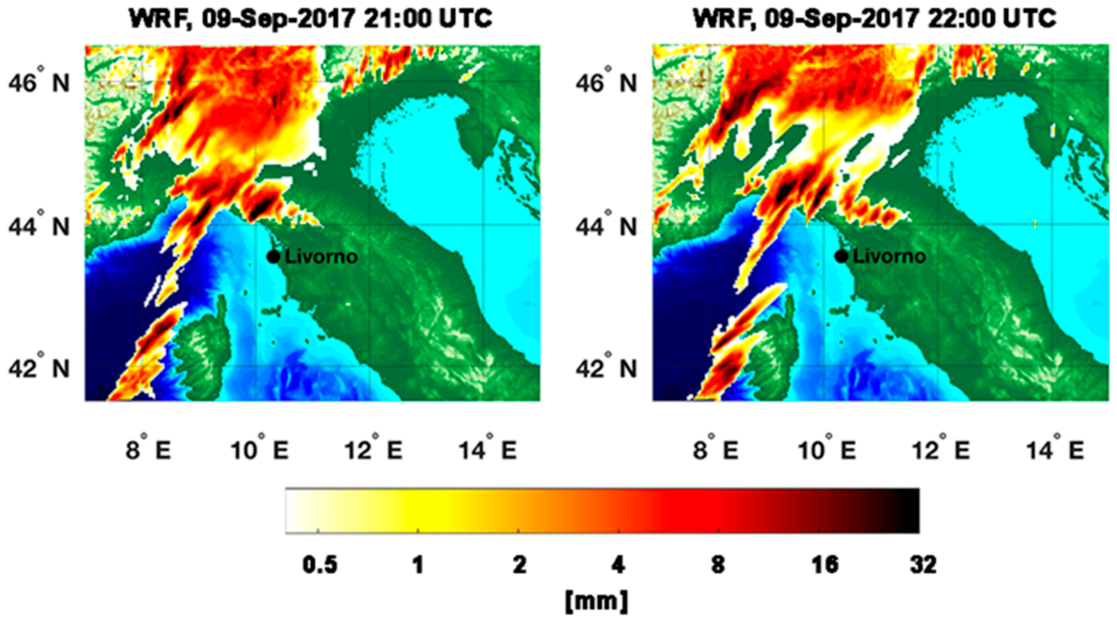
A quantitative evaluation of PET and RainCEIV estimates is performed through a dichotomous statistical assessment. It is important to bear in mind that the PET and Radar RR maps, as well as the RainCEIV RR class map, refers to instantaneous RR values while the WRF RR maps refers to hourly accumulated rainfall. Due to this, we preferred to carry out the quantitative analysis only between instantaneous RR values derived from WRN and from PET and RainCEIV. The dichotomous assessment of PET and RainCEIV is proposed in order to highlight the different performances of the two techniques, and to individuate weakness and strengths and, thus, understand their effectiveness in supporting NWP models. This support could be very useful especially when radar information is not available due to technical problems or partial coverage, e.g., https://www.rainviewer.com/coverage.html (accessed on 2 August 2018). In such cases, the support of satellite-based techniques is vital to forecasters for providing support in managing local alerts. The PET and WRN RR values have been associated to the same RainCEIV RR classes so to have comparable statistics for RainCEIV and PET. Moreover, the radar RR values have been co-located with MSG-SEVIRI, as described in Section 2. In detail, pixels are associated to the class C₀, C₁, or C₂, as defined for RainCEIV [40], when the corresponding RR value satisfies the relation $0\le \mathrm{RR}<0.5\mathrm{mm}{\mathrm{h}}^{-1}$ (C₀, non-rainy class), $0.5\le \mathrm{RR}<4\mathrm{mm}{\mathrm{h}}^{-1}$ (C₁, light to moderate rain class) or $\mathrm{RR}\ge 4\mathrm{mm}{\mathrm{h}}^{-1}$ (C₂, heavy rain class), respectively. This rain classification is arbitrary, and it is based on the observation of rain rate associated to stratiform rain and to convective rain at mid latitudes. In particular, the non-rainy class ranges from 0 mm h⁻¹ to 0.1 or 0.5 mm h⁻¹, because these small values are within the instrument sensitivity and, thus, are included in the non-rainy class. The skill scores used for dichotomous assessment are accuracy, bias score, probability of detection (POD), false alarm ratio (FAR), and Heidke skill score (HSS), described in [61].

Table 2. Contingency table for the dichotomous statistical assessment of RainCEIV for Rainfall Peak A (from 20:30 UTC to 21:30 UTC of 9 September 2017).

		Radar-Derived Rain Rate Results
RainCEIV results		Rain	No rain	Marginal total
	Rain	15,309	8391	23,700
	No rain	3150	25,710	28,860
	Marginal total	18,459	34,101	52,560

and

Table 3. Contingency table for the dichotomous statistical assessment of PET for Rainfall Peak A (from 20:30 UTC to 21:30 UTC of 9 September 2017).

		Radar-Derived Rain Rate Results
PET results		Rain	No rain	Marginal total
	Rain	15,723	3936	19,659
	No rain	2736	30,165	32,901
	Marginal total	18,459	34,101	52,560

summarize the contingency values related to Rainfall Peak A, while the skill scores, calculated for all the classes considered together, as well as for C₁ and C₂ classes separately, are shown in

Table 4. Dichotomous statistical scores (RainCEIV/PET versus radar-derived rain rate measurements) for Rainfall Peak A (from 20:30 UTC to 21:30 UTC of 9 September 2017). The statistical scores are shown for all rainy classes (C₁, C₂), light to moderate rain (C₁), and heavy rain (C₂).

Statistical Scores	C1 (RainCEIV)	C1 (PET)	C2 (RainCEIV)	C2 (PET)	C1, C2 (RainCEIV)	C1, C2 (PET)
Accuracy	0.71	0.85	0.87	0.91	0.78	0.87
Bias	1.79	1.17	1.00	0.30	1.28	1.06
POD	0.71	0.81	0.49	0.28	0.83	0.85
FAR	0.60	0.30	0.51	0.05	0.35	0.20
HSS	0.31	0.65	0.34	0.34	0.55	0.75

for both RainCEIV and PET statistical assessment. For this case study, it is evident that PET performs better than RainCEIV; in fact when classes C₁ and C₂ are considered together, the PET accuracy score (0.87) is higher than that related to RainCEIV (0.78) for all the rainy classes. The bias is slightly higher than 1 for PET (1.06), also showing high POD (0.85) and low FAR (0.20). These scores indicate that PET detects rainy areas with better performances and reduce the overestimation of rainy areas with respect to RainCEIV (bias = 1.28, FAR = 0.35). Although bias is higher for RainCEIV than for PET, due to higher false alarms number for RainCEIV (8391) than PET (3936), POD is high for both the algorithms (0.83 for RainCEIV, 0.85 for PET). HSS is relative to random forecast, and it is based on accuracy corrected by the number of hits that would be expected by chance. HSS can assume values between −1 and 1, and its perfect score is 1, while 0 indicates no skill. HSS values for PET and RainCEIV are 0.75 and 0.55, respectively, demonstrating good performance of the two algorithms in detecting rainy areas and confirming the best performance of PET. The statistical scores related to the C₁ and C₂ classes have been also considered to further analyze the behavior of the two algorithms. In order to better explain the C₁ and C₂ statistical assessment, it is helpful to define the C₁ and C₂ contingency table elements. Specifically, for the dichotomous statistical assessment of C₁/C₂ class, the hits or correct negatives are the pixels for which both the PET/RainCEIV RR class, and the corresponding WRN co-located RR class are C₁/C₂ or C₀ classes, respectively. For the dichotomous statistical assessment of C₁ class, the misses are the pixels for which the WRN co-located RR class is C₁, and the corresponding PET/RainCEIV RR class is C₀, while the false alarms are the pixels for which the PET/RainCEIV RR class is C₁, while the corresponding class is C₀. Finally, for dichotomous statistical assessment of C₂ class, the misses are the pixels for which WRN co-located RR class is C₂, and the corresponding PET/RainCEIV RR class is C₀ or C₁, and the false alarms are the pixels for which PET/RainCEIV RR class is C₂, and the corresponding WRN co-located RR class is C₀ or C₁. The C₁/C₂ accuracy for RainCEIV is 0.71/0.87, which is lower than that of PET (0.85/0.91), consistently with the fact that both hits and correct negatives are higher for PET than for RainCEIV for both the classes. The RainCEIV tendency to overestimate rainy areas is confirmed also for the two classes separately; in fact, the RainCEIV FAR is 0.60 for C₁ and 0.51 for C₂ while the PET FAR is 0.30 and 0.05 for C₁ and C₂ class, respectively. Along with the higher FAR values, RainCEIV shows better performances in detecting rainy pixels belonging both to C₁ and C₂ class. RainCEIV skill in detecting C₂ rainy areas seems better (for Rainfall Peak A) than that of PET: C₂ bias and POD are 1.00 and 0.49 for RainCEIV while 0.30 and 0.28 for PET. This latter result is strongly influenced by the fact that RainCEIV C₂ hits are higher than the PET C₂ hits; on the contrary, C₂ correct negatives are smaller for RainCEIV than for PET, resulting in higher C₂ accuracy for PET (0.91) than for RainCEIV (0.87).

For Rainfall Peak B,

Table 5. Contingency table for the dichotomous statistical assessment of RainCEIV for Rainfall Peak B (from 00:30 UTC to 03:30 UTC of 10 September 2017).

		Radar-Derived Rain Rate Results
RainCEIV results		Rain	No rain	Marginal total
	Rain	16,306	13,412	29,718
	No rain	6950	29,032	35,982
	Marginal total	23,256	42,444	65,700

and

Table 6. Contingency table for the dichotomous statistical assessment of PET for the Rainfall Peak B (from 00:30 UTC to 03:30 UTC of 10 September 2017).

		Radar-Derived Rain Rate Results
PET results		Rain	No rain	Marginal total
	Rain	15,242	6574	21,816
	No rain	8014	35,870	43,884
	Marginal total	23,256	42,444	65,700

summarize the contingency values and

Table 7. Dichotomous statistical scores (RainCEIV/PET versus radar-derived RR measurements) for Rainfall Peak B (from 00:30 UTC to 03:30 UTC of 10 September 2017). The statistical scores are shown for all rainy classes (C₁, C₂), light to moderate rain (C₁), and heavy rain (C₂).

Statistical Scores	C1 (RainCEIV)	C1 (PET)	C2 (RainCEIV)	C2 (PET)	C1, C2 (RainCEIV)	C1, C2 (PET)
Accuracy	0.64	0.73	0.82	0.95	0.69	0.78
Bias	1.56	1.09	1.38	0.83	1.28	0.94
POD	0.52	0.51	0.49	0.69	0.70	0.66
FAR	0.67	0.53	0.64	0.17	0.45	0.30
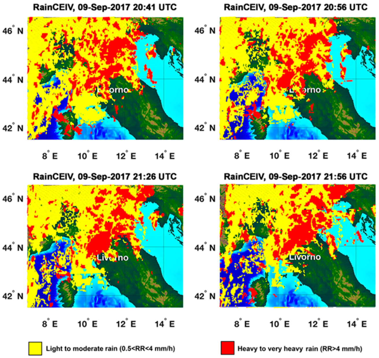
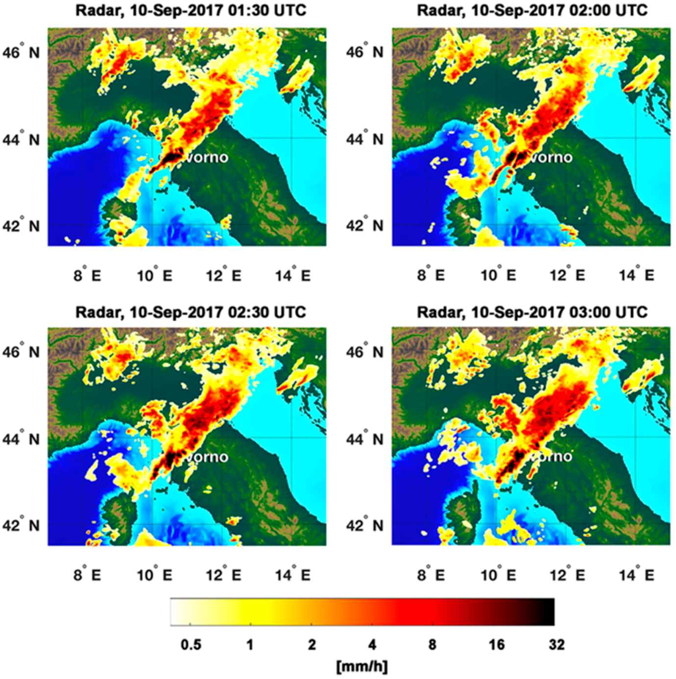
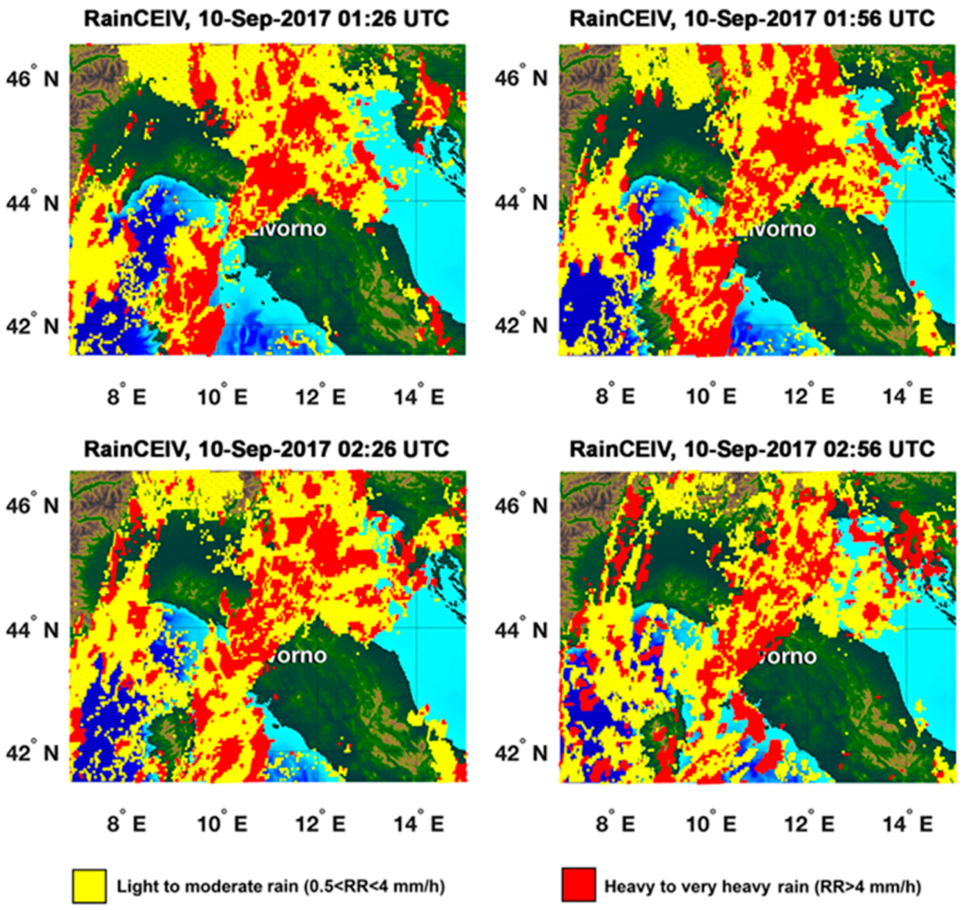
HSS	0.16	0.30	0.22	0.69	0.37	0.51

shows the statistical assessment for all the classes, confirming the good performance of PET (accuracy = 0.78, bias = 0.94, POD = 0.66, FAR = 0.30, HSS = 0.51) for the case study analyzed. The RainCEIV statistical assessment for all the classes reveals accuracy (0.69) and HSS (0.37) skill to be smaller than the corresponding PET statistical scores, the bias (1.28) indicates a tendency in RainCEIV overestimating rainy areas, while POD (0.70) is slightly higher than the PET POD. As evident also by visual comparison of RainCEIV with Radar RR (Section 3.2), it is clear that RainCEIV overestimates rainy areas and, in particular, the C₁ rainy areas (bias = 1.56, FAR = 0.67). 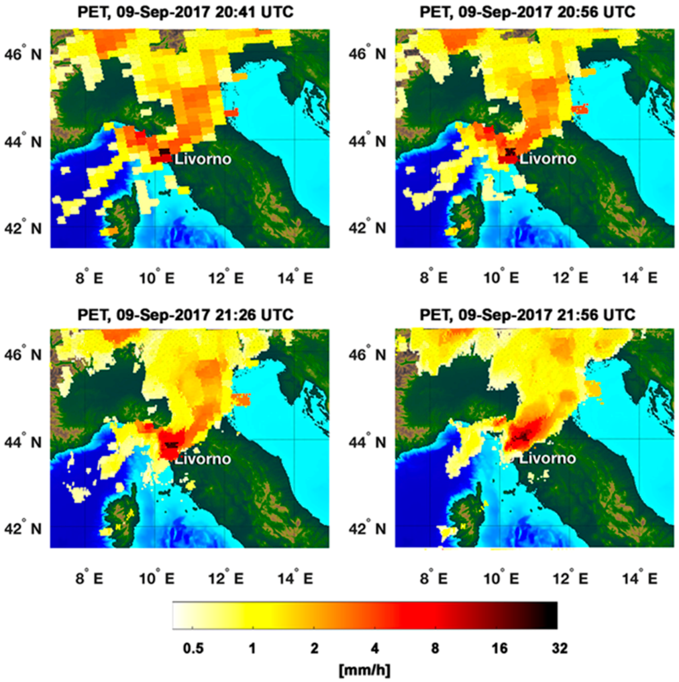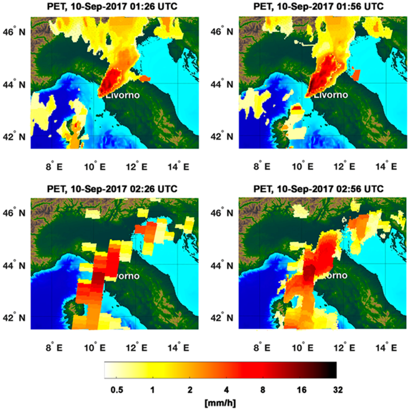For RainCEIV C₂ class, bias (1.38) and FAR (0.64) are slightly better than the C₁ class corresponding values, and when compared with PET C₂ statistical scores, it is possible to note a much smaller FAR (0.17), but also a bias (0.83) that reveals the tendency of PET in underestimating C₂ rainy areas, while this is not the case for C₁ class (bias = 1.09, POD = 0.51). It is evident that, while RainCEIV tendency (overestimation of rainy areas) is the same for the two rainfall peaks, the PET statistical behavior is strongly affected by the fact that at 01:26 UTC and 01:56 UTC PET has been still moving forward the information that corresponds to the 20:42 UTC AMSU initial map. 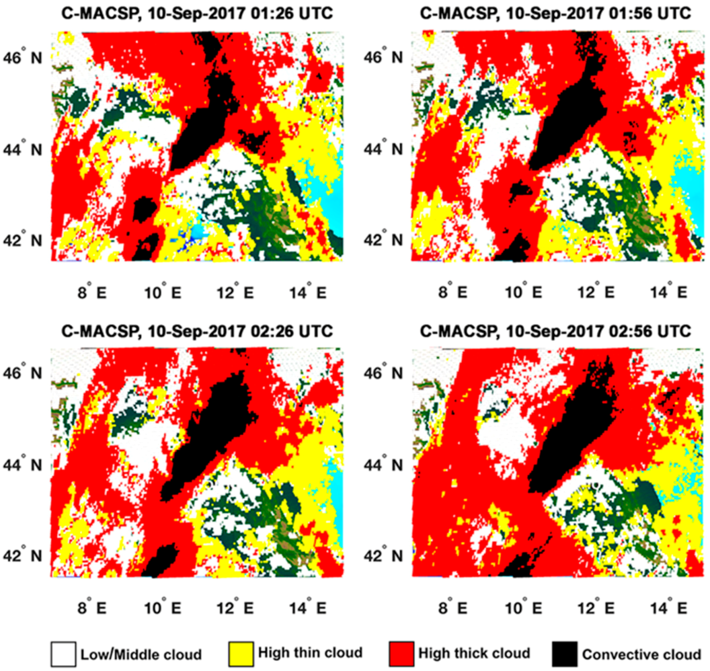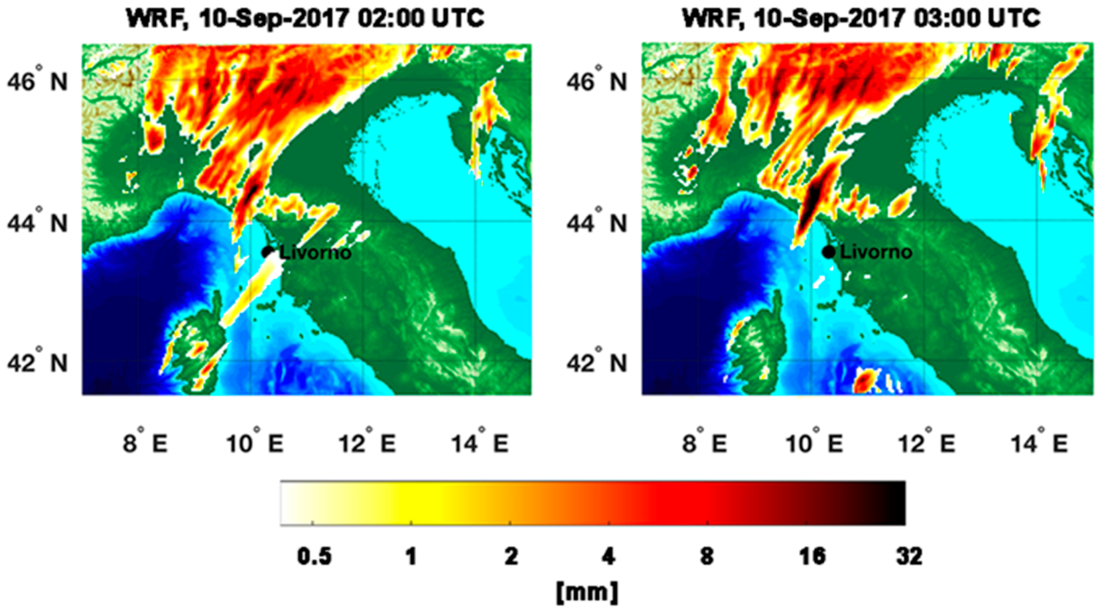This means that the temporal distance from the PMW initialization data is higher than 4 h, while the PET statistical assessment in [39] shows the PET overall ability to propagate rain field at least for 2–3 h. The statistical assessment of RainCEIV and PET is slightly better for Rainfall Peak A than for Rainfall Peak B. This depends on the different developing stages of the storm related to the two peaks. In detail, the storm associated to Rainfall Peak A is composed by convective cells in initial and mature stage whose cloud-tops and the related sub-cloud rain estimations are determined with smaller overestimations than those characterizing the detection of convective cloud top and rain estimations associated with mature and dissipating stages. In fact, the statistical assessment of Rainfall Peak B is strongly influenced by the presence of a large convective activity starting at circa 22:00 UTC northwest Livorno; this is a mix of mature and dissipating stages because of its long duration. The presence of dissipating stage causes the convective cloud top detected by IR to appear larger and, consequently, the rain estimation in sub-cloud area is overestimated. This effect is more evident in RainCEIV than in PET because, in PET, it is mitigated by the direct use of PMW RR.

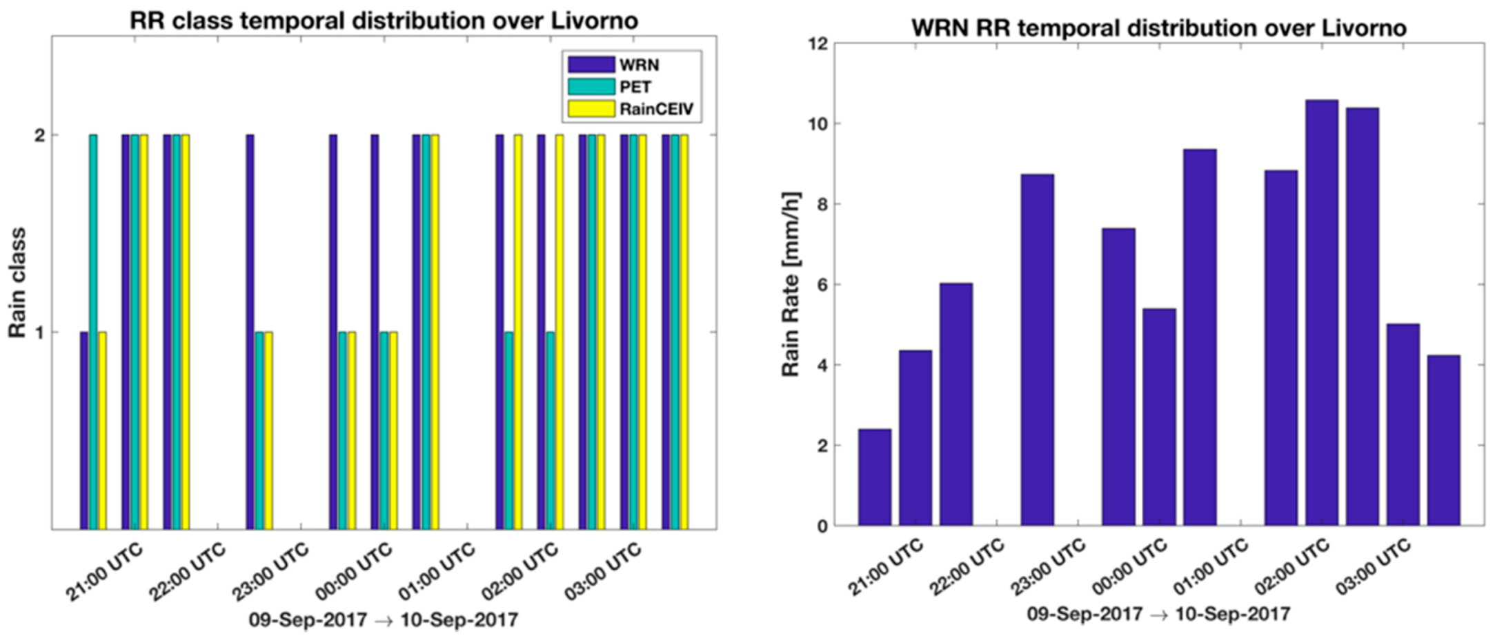
Finally,

Table 8. Contingency table for the dichotomous statistical assessment of PET for the whole storm duration (from 20:30 UTC of 9 September 2017 to 03:30 UTC of 10 September 2017).

		Radar-Derived Rain Rate Results
PET results		Rain	No rain	Marginal total
	Rain	40,142	14,219	54,361
	No rain	12,611	90,708	103,319
	Marginal total	52,753	104,927	157,680

and

Table 9. Contingency table for the dichotomous statistical assessment of RainCEIV for the whole storm duration (from 20:30 UTC of 10 September 2017 to 03:30 UTC of 10 September 2017).

		Radar-Derived Rain Rate Results
RainCEIV results		Rain	No rain	Marginal total
	Rain	40,866	29,448	70,314
	No rain	11,887	75,479	87,366
	Marginal total	52,753	104,927	157,680

show the contingency values related to the whole storm duration (from 21:30 UTC of 10 September 2017 to 03:30 UTC of 10 September 2017) while

Table 10. Dichotomous statistical scores (RainCEIV/PET versus radar -derived RR measurements) for the whole storm duration (from 20:30 UTC of 9 September to 03:30 UTC of 10 September 2017). The statistical scores are shown for both rainy classes (C₁, C₂), light to moderate rain (C₁), and heavy rain (C₂).

Statistical Scores	C1 (RainCEIV)	C1 (PET)	C2 (RainCEIV)	C2 (PET)	C1, C2 (RainCEIV)	C1, C2 (PET)
Accuracy	0.69	0.80	0.85	0.93	0.74	0.83
Bias	1.69	1.16	1.33	0.57	1.33	1.03
POD	0.63	0.69	0.49	0.49	0.77	0.76
FAR	0.62	0.41	0.63	0.13	0.42	0.26
HSS	0.27	0.49	0.25	0.56	0.46	0.62

shows the skill scores, calculated for all the classes considered together, as well as for C₁ and C₂ classes separately, for both RainCEIV and PET statistical assessment. The PET statistical results for all the classes (accuracy = 0.83, POD = 0.76, FAR = 0.26, HSS = 0.62, bias = 1.03) are slightly better than the RainCEIV ones (accuracy = 0.74, POD = 0.77, FAR = 0.42, HSS = 0.46, bias = 1.33), and confirm the RainCEIV tendency in overestimating rainy areas. The statistical scores related to both the algorithms are comparable with the ones obtained by [14], who investigated the reliability of several PMW-based precipitation algorithms [62,63,64,65], obtaining POD values between 0.60–0.76 and FAR between 0.28–0.45, and with the statistical assessment of CMORPH [12], which shows 0.20 < POD < 0.80, 0.15 < FAR < 0.45, and 0.30 < HSS < 0.62.

The proposed satellite-based techniques show their ability in detecting rainy areas and in characterizing them by using cloud type information from C_MACSP. RainCEIV and PET, providing near-real-time estimations of RR and RR classes at the MSG-SEVIRI temporal and spatial resolution (i.e., about 15 min and (5 × 7) km² at mid-latitude), show different performance for both rainfall peaks. Compared to WRN RR, we found better agreement with PET than with RainCEIV, which is attributable to the different way the two techniques deal with the information from PMW RR. In fact, PET propagates forward, in space and in time, the last available PMW RR map that gives direct information on the event to analyze. This influences the slightly worse PET performance in Rainfall Peak B. In fact, it is a consequence of the different delay from the last available PMW observation (PMW delay) used to initialize PET in the two Peaks. In detail, PMW delay is about 1 h for Rainfall Peak A and about 4 h for the 01:26 UTC and 01:56 UTC PET maps of Rainfall Peak B, producing a higher RR overestimation in Peak B than in Peak A. On the contrary, no direct information on the actual rainfall distribution is provided to RainCEIV. The only PMW information that RainCEIV uses is within the training dataset built on a series of PMW RR maps from previous rainfall events. However, in spite of its worse statistical scores, RainCEIV is able to give information on rain class without temporal and spatial limitations (within the observed Earth’s disk), while PET produces RR maps for only a few hours after the last available PMW observations, and only on the region around the PMW swath observations. From the qualitative analysis and statistical assessment, it is evident that the three techniques are complementary in supporting the WRF model forecasting, especially for real-time continuous monitoring of convective events. In particular, PET can provide information about RR for about three hours from the last PMW RR map available on the area of interest, while RainCEIV and C_MACSP can give information about RR class and cloud type with no limitation of space and time within the observed Earth’s disk. When available, PET RR information is preferable to the RainCEIV RR class information. On the other hand, RainCEIV RR class information is useful when PET is not available. For the case study examined in this paper, the information from the three satellite-based techniques could appear redundant as a support for the NWP forecast, because of the availability of WRN-derived RR. In any case, the aim of the analysis presented is to highlight the effectiveness of the satellite techniques as a valid support for NWP forecast, especially when there is no WRN information.

5. Conclusions

The prediction of the intense precipitation that hit central Italy on 9 and 10 September 2017 did not help to avoid the tragic events and serious damage to the local infrastructure in the city of Livorno, although it was forecast by several NWP models. Precipitation was intense everywhere in Tuscany; DPC alerted the whole region at the same level, though Livorno was the only city heavily affected, prevalently for reasons related to the urban development near Rio Maggiore. In this paper, the event has been analyzed by means of remote sensing techniques, to investigate their effectiveness in continuous monitoring of extreme events and their utility in supporting NWP forecast. To this end, precipitation maps from the WRF model forecast have also been analyzed. All the three remote sensing techniques used in this study exploit the high spatial and temporal resolution of MSG-SEVIRI, in order to give information about the cloud classification (C-MACSP), the RR class (RainCEIV), and the RR values (PET). These techniques use the RR information retrieved by the PMW observations differently, and this affects their performance. In detail, PET exploits the latest PMW observations directly, and it provides RR map values every 15 min on the area limited to the PMW swath and for a few hours. On the contrary, RainCEIV and C-MACSP indirectly use the PMW RR maps to build the training dataset, which is not updated with the most recent information on the raining area distribution. RainCEIV RR class maps and C-MACSP cloud classification maps are available every 15 min without temporal and spatial limitation within the Earth’s disk, observed by GEO orbit. It is evident that C-MACSP, PET, and RainCEIV are complementary for the real-time monitoring of extreme events. In fact, C-MACSP gives information about cloud cover and cloud type, while PET and RainCEIV give RR quantitative and qualitative information, respectively. Due to the abovementioned PET temporal and spatial limitations, PET RR values are not always available and, in this case, RainCEIV RR class information, although less efficient than PET quantitative information, is very useful in order to detect and characterize rainy areas. The techniques agree with WRN-RR maps in detecting rainy areas, as confirmed by the qualitative analysis for both A and B rainfall peak. Moreover, the statistical scores determined for the Rainfall Peaks A/B and for the entire of the event’s duration (from 20:30 UTC of 9 September to 03:30 UTC of 10 September 2017) indicate good performances of PET and RainCEIV (for PET: accuracy = 0.82, bias = 1.03, POD = 0.76, FAR = 0.26, HSS = 0.62; for RainCEIV: accuracy = 0.74, bias = 1.33, POD = 0.77, FAR = 0.41, HSS = 0.46). In fact, the bias and FAR are higher for RainCEIV (1.33 and 0.41, respectively) than for PET (bias = 1.03, FAR = 0.26), denoting a tendency to overestimate the extent of rainy areas for RainCEIV. The WRF hourly accumulated precipitation maps do not detect heavy precipitation in Livorno and its surroundings in any of the rainfall peaks analyzed. The three satellite techniques could be very useful for the real-time monitoring purposes, especially when the forecast is not correct and the WRN data are not available as support for forecasters. Clearly, MACSP, PET, and RainCEIV cannot replace the NWP maps in foreseeing the precipitation area, but they can be very useful to characterize the area and observe the severe weather in real-time, especially for the cases in which WRN RR information is missing. In particular, RainCEIV RR class maps are to be used when the PET RR maps are not available, whereas C-MACSP gives information about cloud cover and can be useful to detect areas with high probability for deep convection.

References

1. Pregnolato, M.; Sean, A.F.; Wilkinson, M.; Dawson, R.J. The impact of flooding on road transport: A depth-disruption function. Transp. Res. 2017, 55, 67–81. [Google Scholar] [CrossRef]
2. Mecikalski, J.R.; Berendes, T.A.; Feltz, W.F.; Bedka, K.M.; Bedka, S.T.; Murray, J.J.; Wimmers, A.J.; Minnis, P.; Johnson, D.B.; Haggerty, J.; et al. Aviation Applications for Satellite-Based Observations of Cloud Properties, Convection Initiation, In-Flight Icing, Turbulence, and Volcanic Ash. Bull. Am. Meteorol. Soc. 2007, 88, 1589–1607. [Google Scholar] [CrossRef] [Green Version]
3. Murray, J.J. Aviation weather applications of Earth Science Enter- prise data. Earth Obs. Mag. 2002, 11, 27–30. [Google Scholar]
4. Cuo, L.; Pagano, T.C.; Wang, Q.J. A review of quantitative precipitation forecasts and their use in short- to medium-range streamflow forecasting. J. Hydrometeorol. 2011, 12, 713–728. [Google Scholar] [CrossRef]
5. Merk, D.; Zinner, T. Detection of convective initiation using Meteosat SEVIRI: Implementation in and verification with the tracking and nowcasting algorithm Cb-TRAM. Atmos. Meas. Tech. 2013, 6, 1903–1918. [Google Scholar] [CrossRef]
6. Zinner, T.; Mannstein, H.; Tafferner, A. Cb-TRAM: Tracking and monitoring severe convection from onset over rapid devel- opment to mature phase using multi-channel Meteosat-8 SEVIRI data. Meteorol. Atmos. Phys. 2008, 101, 191–210. [Google Scholar] [CrossRef] [Green Version]
7. Zinner, T.; Forster, C.; de Coning, E.; Betz, H.-D. Validation of the Meteosat storm detection and nowcasting system Cb-TRAM with lightning network data—Europe and South Africa. Atmos. Meas. Tech. 2013, 6, 1567–1583. [Google Scholar] [CrossRef] [Green Version]
8. Mecikalski, J.R.; Bedka, K.M. Forecasting Convective Initiation by Monitoring the Evolution of Moving Cumulus in Day- time GOES Imagery. Mon. Weather Rev. 2006, 134, 49–78. [Google Scholar] [CrossRef]
9. Li, Z.; Li, J.; Wang, P.; Lim, A.; Li, J.; Schmit, T.J.; Atlas, R.; Boukabara, S.A.; Hoffman, R.F. Value-added Impact of Geostationary Hyperspectral Infrared Sounders on Local Severe Storm Forecasts via a Quick Regional OSSE. Adv. Atmos. Sci. 2018, 35, 1217–1230. [Google Scholar] [CrossRef]
10. Ai, Y.; Li, J.; Shi, W.; Schmit, T.J.; Cao, C.; Li, W. Deep convective cloud characterizations from both broadband imager and hyperspectral infrared sounder measurements. J. Geophys. Res. Atmos. 2017, 122, 1700–1712. [Google Scholar] [CrossRef]
11. Neto, C.P.S.; Barbosa, H.A.; Beneti, C.A.A. A method for convective storm detection using satellite data. Atmósfera 2016, 29, 343–358. [Google Scholar] [CrossRef] [Green Version]
12. Joyce, R.J.; Janowiak, J.E.; Arkin, P.A.; Xie, P. Cmorph: A method that produces global precipitation estimates from passive microwave and infrared data at high spatial and temporal resolution. J. Hydrometeorol. 2004, 5, 487–503. [Google Scholar] [CrossRef]
13. Joyce, R.J.; Xie, P. Kalman filter–based cmorph. J. Hydrometeorol. 2011, 12, 1547–1563. [Google Scholar] [CrossRef]
14. Panegrossi, G.; Casella, D.; Dietrich, S.; Marra, A.C.; Sanò, P.; Mugnai, A.; Baldini, L.; Roberto, N.; Adirosi, E.; Cremonini, R.; et al. Use of the GPM Constellation for Monitoring Heavy Precipitation Events over the Mediterranean Region. IEEE J. Select. Top. Appl. Earth Obs. Remote Sens. 2016, 9, 2733–2753. [Google Scholar] [CrossRef]
15. Di Paola, F.; Ricciardelli, E.; Cimini, D.; Romano, F.; Viggiano, M.; Cuomo, V. Analysis of Catania Flash Flood Case Study by Using Combined Microwave and Infrared Technique. J. Hydrometeorol. 2014, 15, 1989–1998. [Google Scholar] [CrossRef]
16. He, Y.; Zhang, Y.; Kuligowski, R.; Cifelli, R.; Kitzmiller, D. Incorporating Satellite Precipitation Estimates into a Radar-Gauge Multi-Sensor Precipitation Estimation Algorithm. Remote Sens. 2018, 10, 106. [Google Scholar] [CrossRef]
17. Huang, Y.; Meng, Z.; Li, J.; Li, W.; Bai, L.; Zhang, M.; Wang, X. Distribution and Variability of Satellite-Derived Signals of Isolated Convection Initiation Events over Central Eastern China. J. Geophys. Res. Atmos. 2017, 122, 21. [Google Scholar] [CrossRef]
18. Weng, F.; Grody, N.C. Retrieval of ice cloud parameters using a microwave imaging radiometer. J. Atmos. Sci. 2000, 57, 1069–1081. [Google Scholar] [CrossRef]
19. Bennartz, R.; Petty, G.W. The sensitivity of microwave remote sensing observations of precipitation to ice particle size distributions. J. Appl. Meteorol. 2001, 40, 345–364. [Google Scholar] [CrossRef]
20. Grody, N.; Zhao, J.; Ferraro, R.; Weng, F.; Boers, R. Determination of precipitable water and cloud liquid water over oceans from the NOAA 15 Advanced Microwave Sounding Unit. J. Geophys. Res. 2001, 106. [Google Scholar] [CrossRef]
21. Bonsignori, R. The Microwave Humidity Sounder (MHS): In-orbit performance assessment. Proc. SPIE 2007, 6744, 6744. [Google Scholar] [CrossRef]
22. Ferraro, R.R.; Weng, F.; Grody, N.C.; Zhao, L.; Meng, H.; Kongoli, C.; Pellegrino, P.; Qiu, S.; Dean, C. NOAA operational hydrological products derived from the Advanced Microwave Sounding Unit. IEEE Trans. Geosci. Remote Sens. 2005, 43, 1036–1049. [Google Scholar] [CrossRef]
23. Wilcox, E.M.; Donner, L.J. The frequency of extreme rain events in satellite rain-rate estimates and an atmospheric general circulation model. J. Clim. 2007, 20, 53–69. [Google Scholar] [CrossRef]
24. Wardah, T.; Abu Bakar, S.H.; Bardossy, A.; Maznorizan, M. Use of geostationary meteorological satellite images in convective rain estimation for flash-flood forecasting. J. Hydrol. 2008, 356, 283–298. [Google Scholar] [CrossRef]
25. Kummerow, C.D.; Ringerud, S.; Crook, J.; Randel, D.; Berg, W. An observationally generated a priori database for microwave rainfall retrievals. J. Atmos. Ocean. Technol. 2010, 28, 113–130. [Google Scholar] [CrossRef]
26. Bennartz, R.; Schroeder, M. Convective activity over Africa and the tropical Atlantic inferred from 20 years of geostationary Meteosat infrared observations. J. Clim. 2012, 25, 156–169. [Google Scholar] [CrossRef]
27. Wu, H.; Adler, R.F.; Hong, Y.; Tian, Y.; Policelli, F. Evaluation of global flood detection using satellite-based rainfall and a hydrologic model. J. Hydrometeorol. 2012, 13, 1268–1284. [Google Scholar] [CrossRef]
28. Casella, D.; Dietrich, S.; di Paola, F.; Formenton, M.; Mugnai, A.; Porcù, F.; Sanò, P. PM-GCD—A combined IR–MW satellite technique for frequent retrieval of heavy precipitation. Nat. Hazards Earth Syst. Sci. 2012, 12, 231–240. [Google Scholar] [CrossRef] [Green Version]
29. Sanò, P.; Panegrossi, G.; Casella, D.; Di Paola, F.; Milani, L.; Mugnai, A.; Petracca, M.; Dietrich, S. The passive microwave Neural network Precipitation Retrieval (PNPR) algorithm for AMSU/MHS observations: Description and application to European case studies. Atmos. Meas. Tech. 2015, 8, 837–857. [Google Scholar] [CrossRef]
30. Adler, R.F.; Negri, A.J. A satellite infrared technique to estimate tropical convective and stratiform rainfall. J. Appl. Meteorol. 1988, 27, 30–51. [Google Scholar] [CrossRef]
31. Adler, R.F.; Markus, M.J.; Fenn, D.D. Detection of severe Midwest thunderstorms using geosynchronous satellite data. Mon. Weather Rev. 1985, 113, 769–781. [Google Scholar] [CrossRef]
32. Wu, R.; Weinman, J.A.; Chin, R.T. Determination of rainfall rates from GOES satellite images by a pattern recognition technique. J. Atmos. Ocean. Technol. 1985, 2, 314–330. [Google Scholar] [CrossRef]
33. Adler, R.F.; Negri, A.J.; Keehn, P.R.; Hakkarinen, I.M. Estimation of monthly rainfall over Japan and surrounding waters from a combination of low-orbit microwave and geosynchronous IR data. J. Appl. Meteorol. 1993, 32, 335–356. [Google Scholar] [CrossRef]
34. Jobard, I.; Desbois, M. Satellite estimation of the tropical precipitation using the Meteosat and SSM/I data. Atmos. Res. 1994, 34, 285–298. [Google Scholar] [CrossRef]
35. Turk, J.F.; Rohaly, G.; Hawkins, J.; Smith, E.A.; Marzano, F.S.; Mugnai, A.; Levizzani, V. Meteorological applications of precipitation estimation from combined SSM/I, TRMM, and geostationary satellite data. In Microwave Radiometry and Remote Sensing of the Environment; Pampaloni, P., Ed.; VSP Intern. Sci. Publisher: Utrecht, The Netherlands, 2000; pp. 353–363. [Google Scholar]
36. Kidd, C.; Kniveton, D.R.; Todd, M.C.; Bellerby, T.J. Satellite rainfall estimation using a combined passive microwave and infrared algorithm. J. Hydrometeorol. 2003, 4, 1088–1104. [Google Scholar] [CrossRef]
37. Marzano, F.S.; Palmacci, M.; Cimini, D.; Giuliani, G.; Turk, J.F. Multivariate Statistical Integration of Satellite Infrared and Microwave Radiometric Measurements for Rainfall Retrieval at the Geostationary Scale. IEEE Trans. Geosci. Remote Sens. 2004, 42, 1018–1032. [Google Scholar] [CrossRef]
38. Heinemann, T.; Lattanzio, A.; Roveda, F. The Eumetsat multi- sensor precipitation estimate (MPE). In Proceedings of the Second International Precipitation Working Group (IPWG) Meeting, Madrid, Spain, 23–27 September 2002. [Google Scholar]
39. Di Paola, F.; Casella, D.; Dietrich, S.; Mugnai, A.; Ricciardelli, E.; Romano, F.; Sanoò, P. Combined MW-IR Precipita- tion Evolving Technique (PET) of convective rain fields. Nat. Hazards Earth Syst. Sci. 2012, 12, 3557–3570. [Google Scholar] [CrossRef] [Green Version]
40. Ricciardelli, E.; Cimini, D.; Di Paola, F.; Romano, F.; Viggiano, M.A. Statistical approach for rain intensity differentiation using Meteosat second generation-spinning enhanced visible and infrared imager observations. Hydrol. Earth Syst. Sci. 2014, 18, 2559–2576. [Google Scholar] [CrossRef] [Green Version]
41. Ricciardelli, E.; Romano, F.; Cuomo, V. Physical and statistical approaches for cloud identification using Meteosat Second Generation-Spinning Enhanced Visible and Infrared Imager Data. Remote Sens. Environ. 2008, 112, 2741–2760. [Google Scholar] [CrossRef]
42. Nilo, S.T.; Romano, F.; Cermak, J.; Cimini, D.; Ricciardelli, E.; Cersosimo, A.; Di Paola, F.; Gallucci, D.; Gentile, S.; Geraldi, E.; et al. Fog Detection Based on Meteosat Second Generation-Spinning Enhanced Visible and InfraRed Imager High Resolution Visible Channel. Remote Sens. 2018, 10, 541. [Google Scholar] [CrossRef]
43. Ricciardelli, E.; Di Paola, F.; Cimini, D.; Romano, F.; Viggiano, M. Satellite Remote Sensing for clouds and precipitation. In Advances in Watershed Hydrology; Water Resource Publications, LLC: Littleton, CO, USA, 2015; pp. 69–82. ISBN 154-196, 978-1-887201-85-8. [Google Scholar]
44. Schmetz, J.; Pili, P.; Tjemkes, S.; Just, D.; Kerkmann, J.; Rota, S.; Ratier, A. An Introduction to Meteosat Second Generation (MSG). Bull. Am. Meteorol. Soc. 2002, 83, 977–992. [Google Scholar] [CrossRef]
45. Di Tomaso, E.; Romano, F.; Cuomo, V. Rainfall estimation from satellite passive microwave observations in the range 89 GHz to 190 GHz. J. Geophys. Res. 2009, 114, D18203. [Google Scholar] [CrossRef]
46. Cimini, D.; Romano, F.; Ricciardelli, E.; Di Paola, F.; Viggiano, M.; Marzano, F.S.; Colaiuda, V.; Picciotti, E.; Vulpiani, G.; Cuomo, V. Validation of satellite OPEMW precipitation product with ground-based weather radar and rain gauge networks. Atmos. Meas. Tech. 2013, 6, 3181–3196. [Google Scholar] [CrossRef] [Green Version]
47. Kramer, H.J. Observation of the Earth and Its Environment; Springer: Berlin, Germany, 2002; p. 1510. [Google Scholar]
48. Kleespies, T.J.; Watts, P. Comparison of simulated radiances, jacobians and linear error analysis for the Microwave Humidity Sounder and the Advanced Microwave Sounding Unit-B. Q. J. R. Meteorol. Soc. 2007, 132, 3001–3010. [Google Scholar] [CrossRef]
49. Ebert, E. A pattern recognition technique for distinguishing surface and cloud types in the polar regions. J. Clim. Appl. Meteorol. 1987, 26, 1412–1427. [Google Scholar] [CrossRef]
50. Parikh, J. A comparative Study of Cloud Classification Techniques. Remote Sens. Environ. 1977, 6, 67–81. [Google Scholar] [CrossRef]
51. Vulpiani, G.; Pagliara, P.; Negri, M.; Rossi, L.; Gioia, A.; Giordano, P.; Alberoni, P.P.; Cremonini, R.; Ferraris, L.; Marzano, F.S. The Italian radar network within the national early-warning system for multi-risks management. In Fifth European Conference on Radar in Meteorology and Hydrology (ERAD 2008); Finnish Meteorological Institute: Helsinki, Finland, 2008. [Google Scholar]
52. Vulpiani, G.; Montopoli, M.; Delli Passeri, L.; Gioia, A.G.; Giordano, P.; Marzano, F.S. On the Use of Dual- Polarized C-Band Radar for Operational Rainfall Retrieval in Mountainous Areas. J. Appl. Meteorol. Climatol. 2012, 51, 405–425. [Google Scholar] [CrossRef]
53. MSG Level 1.5 Image Data Format Description. 2017. Available online: https://www.eumetsat.int/website/home/Data/TechnicalDocuments/index.html (accessed on 12 July 2018).
54. Skamarock, W.C.; Joseph, B.K.; Dudhia, J.; Gill, D.O.; Barker, D.M.; Duda, M.G.; Huang, X.Y.; Wang, W.; Powers, J.G. A Description of the Advanced Research WRF Version 3; NCAR: Boulder, CO, USA, 2008. [Google Scholar]
55. Thompson, G.; Eidhammer, T. A study of aerosol impacts on clouds and precipitation development in a large winter cyclone. J. Atmos. Sci. 2014, 71, 3636–3658. [Google Scholar] [CrossRef]
56. Janjic, Z.I.; Gerrity, J.P., Jr.; Nickovic, S. An alternative approach to nonhydrostatic modeling. Mon. Weather Rev. 2001, 129, 1164–1178. [Google Scholar] [CrossRef]
57. Mellor, G.L.; Yamada, T. Development of a turbulence closure model for geophysical fluid problems. Rev. Geophys. 1982, 20, 851–875. [Google Scholar] [CrossRef]
58. Iacono, M.J.; Delamere, J.S.; Mlawer, E.J.; Shephard, M.W.; Clough, S.A.; Collins, W.D. Radiative forcing by long-lived greenhouse gases: Calculations with the AER radiative transfer models. J. Geophys. Res. 2008, 113, D13103. [Google Scholar] [CrossRef]
59. Catto, J.L.; Jakob, C.; Nicholls, N. Can the CMIP5 models represent winter frontal precipitation? Geophys. Res. Lett. 2015. [Google Scholar] [CrossRef]
60. Comellas, A.; Llasat, M.C.; Molini, L.; Parodi, A.; Siccardi, F. Severe rainfall prediction systems for civil protection purposes. In Proceedings of the 12th EGU Plinius Conference on Mediterranean Storms Plinius Conference Abstracts, Corfu, Greece, 1–4 September 2010. [Google Scholar]
61. Ebert, E. Forecast Verification Issues, Methods and FAQ. Available online: http://www.cawcr.gov.au/projects/verification/ (accessed on 12 July 2018).
62. Casella, D.; Panegrossi, G.; Sano, P.; Dietrich, S.; Mugnai, A.; Smith, E.A.; Tripoli, G.J.; Formenton, M.; Di Paola, F.; Leung, W.-Y.H.; et al. Transitioning from CRD to CDRD in Bayesian retrieval of rainfall from satellite overcoming database profile selection ambiguity by consideration of meteorological control on microphysics. IEEE Trans. Geosci. Remote Sens. 2013, 51, 4650–4671. [Google Scholar] [CrossRef]
63. Sanò, P.; Casella, D.; Mugnai, A.; Schiavon, G.; Smith, E.A.; Tripoli, G.J. Transitioning from CRD to CDRD in Bayesian retrieval of rainfall from satellite passive microwave measurements: Part 1. Algorithm description and testing. IEEE Trans. Geosci. Remote Sens. 2013, 51, 4119–4143. [Google Scholar] [CrossRef]
64. Mugnai, A.; Smith, E.A.; Tripoli, G.J.; Bizzarri, B.; Casella, D.; Dietrich, S.; Di Paola, F.; Panegrossi, G.; Sanò, P. CDRD and PNPR satellite passive microwave precipitation retrieval algorithms: EuroTRMM/EURAINSAT origins and H-SAF operations. Nat. Hazards Earth Syst. Sci. 2013, 13, 887–912. [Google Scholar] [CrossRef] [Green Version]
65. Global Precipitation Measurement (GPM) Mission Algorithm Theoretical Basis Document Version 1.4 (GPROF2014 Conical Version Running at the PPS). Available online: http://rain.atmos.colostate.edu/ATBD/ATBD_GPM_Aug1_2014.pdf (accessed on 3 September 2018).
Figure 1. (a) Synoptic analysis at 00:00 UTC, 10 September 2017: European Centre for Medium-Range Weather Forecasts (ECMWF) 500 hPa geopotential height (white lines) and ECMWF mean sea level pressure; (b) Synoptic analysis at 18:00 UTC, 9 September 2017: ECMWF 850 hPa specific humidity (g/kg) and horizontal wind (speed greater than 20 m/s) at 700 hPa by ECMWF (barbs); (c) Synoptic analysis at 18:00 UTC, 9 September 2017: ECMWF 925 hPa temperature (°C) and horizontal wind at 925 hPa by ECMWF (barbs); (d) Synoptic analysis at 18:00 UTC, 9 September 2017: ECMWF height in hPa, where the potential vorticity (PV) equals 1.5 PV units and water vapor channel 6.2 µm of MSG—source: https://www.eumetrain.org.
Remotesensing 10 01549 g001aRemotesensing 10 01549 g001b
Figure 2. WRN (Weather Radar Network) rain rate maps for 9 September 2017 from 20:30 (left) to 22:00 (right).
Remotesensing 10 01549 g002
Figure 3. C-MACSP (cloud Classification–MAsk Coupling of Statistical and Physical methods) maps for 9 September 2017 from 20:26 UTC to 21:56 UTC (Rainfall Peak A).
Remotesensing 10 01549 g003
Figure 4. RainCEIV (Rain Class Evaluation from Infrared and Visible observations) maps for 9 September 2017 from 20:41 UTC to 21:56 UTC (Rainfall Peak A).
Remotesensing 10 01549 g004
Figure 5. PET (Precipitation Evolving Technique) maps for 9 September 2017 from 20:41 UTC to 21:56 UTC (Rainfall Peak A). The spatial resolution appears coarser in the first PET RR map (20:41 UTC); this is due to the direct resampling of the 20:41 UTC PMW RR map into the MSG-SEVIRI grid without applying the PET modules. PET modules have been applied subsequently, giving better spatial resolution to the following images.
Remotesensing 10 01549 g005
Figure 6. WRN RR maps for 10 September 2017 from 01:30 UTC to 03:00 UTC: Rainfall Peak B over Livorno.
Remotesensing 10 01549 g006
Figure 7. C-MACSP maps for 10 September 2017 from 01:26 UTC to 02:56 UTC (Rainfall Peak B).
Remotesensing 10 01549 g007
Figure 8. RainCEIV maps for 10 September 2017 from 01:26 UTC to 02:56 UTC (Rainfall Peak B).
Remotesensing 10 01549 g008
Figure 9. PET maps for 10 September 2017 from 01:26 UTC to 02:56 UTC (Rainfall Peak B). The coarser resolution of the 02:26 UTC is due to the fact that PET has been re-initialized by using the PMW RR information available at 02:26 UTC.
Remotesensing 10 01549 g009
Figure 10. Temporal intervals distributions of WRN, PET, and RainCEIV RR classes (left panel) and WRN RR temporal distribution (right panel) over Livorno from 20:30 UTC of 9 September 2017 to 03:30 UTC of 10 September 2017.
Remotesensing 10 01549 g010
Figure 11. WRF (Weather Research and Forecasting) rainfall accumulated maps for 9 September 2017 at 21:00 UTC and 22:00 UTC.
Remotesensing 10 01549 g011
Figure 12. WRF rainfall accumulated maps for 10 September 2017 at 02:00 UTC and 03:00 UTC.
Remotesensing 10 01549 g012