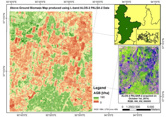
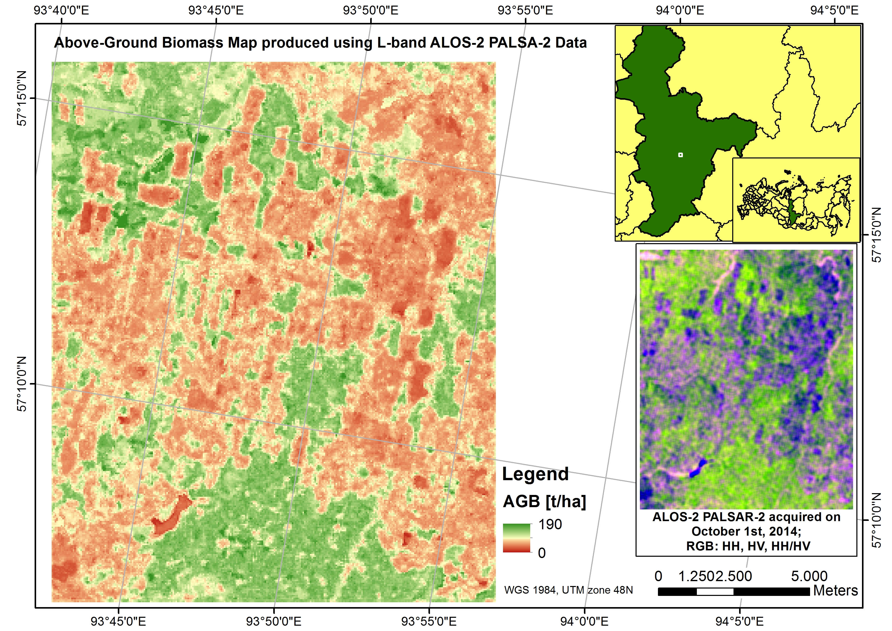
Estimation of Above-Ground Biomass over Boreal Forests in Siberia Using Updated In Situ, ALOS-2 PALSAR-2, and RADARSAT-2 Data

Abstract

The estimation of above-ground biomass (AGB) in boreal forests is of special concern as it constitutes the highest carbon pool in the northern hemisphere. Particularly, monitoring of the forests in the Russian Federation is important as some regions have not been inventoried for many years. This study explores the combination of multi-frequency, multi-polarization, and multi-temporal radar data as one key approach to provide an accurate estimate of forest biomass. The data from L-band Advanced Land Observing Satellite 2 (ALOS-2) Phased Array L-Band Synthetic Aperture Radar 2 (PALSAR-2), together with C-band RADARSAT-2 data, were applied for AGB estimation. Backscatter coefficients from L- and C-band radar were used independently and in combination with a non-parametric model to retrieve AGB data for a boreal forest in Siberia (Krasnoyarskiy Kray). AGB estimation was performed using the random forests machine learning algorithm. The results demonstrated that high estimation accuracies can be achieved at a spatial resolution of 0.25 ha. When the L-band data alone were used for the retrieval, a corrected root-mean-square error (RMSE_cor) of 29.4 t ha⁻¹ was calculated. A marginal decrease in RMSE_cor was observed when only the filtered L-band backscatter data, without ratio and texture, were used (29.1 t ha⁻¹). The inclusion of the C-band data reduced the over and underestimation; the bias was reduced from 5.5 t ha⁻¹ to 4.7 t ha⁻¹; and a RMSE_cor of 30.2 t ha⁻¹ was calculated.

1. Introduction

The importance of forests and above-ground forest biomass (AGB) are manifold. On the one hand, they strongly influence climate change as they act as a carbon sink taking part in the global carbon cycle. However, on the other hand, they are essential to the economy as a source of renewable energy and valuable forest products such as wood, paper, and pulp. Since one-third of the total forest area is used for production purposes, forest policies rely on quantitative estimates of the current and future forest biomass.

Above-ground biomass is defined as the amount of all organic matter growing above ground per unit area at a particular time (t ha⁻¹, Mg ha⁻¹ or kg m⁻²) [1]. It is an essential climate variable [2] that is applied in climate-related global vegetation models [3]. In forestry, the total tree AGB is measured either from ground measurements by felling a tree or using tree-level regression models [4]. The models are based on the allometric relation between biomass and tree elements such as the height and/or diameter at the breast height (dbh). However, due to the sampling nature of the field measurements, and their high acquisition costs, they are limited in time and space. The measurements are carried out by the national forest inventories which are afterwards used for producing forest policies at local, regional, and national levels. Furthermore, the national forest inventories are obligated to report the distribution of the forest AGB to the Food and Agriculture Organization of the United Nations (FAO) as per the Global Forest Resources Assessment (FRA) [5]. The estimation of AGB in boreal forests is of special concern as it constitutes the highest carbon pool in the northern hemisphere. The total forest carbon in boreal forests in Asia was estimated to be 22.1 ± 8.3 Pg C, with a mean carbon density of 4.00 ± 1.54 kg C m⁻² [6]. Data collection for the FRA 2020 has begun in 2018, even though in many countries up-to-date quantitative estimates on the AGB are not available. For example, in the Russian Federation, which has the largest forest area in the world, some forest regions have not been recorded for more than 25 years [7]. At the same time, due to more frequent fires and illegal logging, (which is estimated to make up approximately 20% of all logging activity in Russia), according to the World Bank and the World Wide Fund for Nature (WWF) [8], the AGB experiences dynamic change within a given period of time. Therefore, it is crucial to support national efforts in providing accurate and up-to-date AGB estimates. This can be achieved by means of e earth observation techniques. Even though remote sensing does not provide a direct measurement of AGB, satellite technology together with prior information, e.g., insitu measurements, allow accurate and relatively cost-efficient AGB estimates. In particular, synthetic aperture radar (SAR) systems are of interest as they provide systematic, weather and sun independent observations. Moreover, SAR shows higher sensitivity to AGB in comparison with the optical sensors [9]. The latest results of biomass estimation using optical data (Landsat) showed measures of moderate accuracy, with a relative mean absolute error (rMAE) of approximately 36%, in the boreal zone [10].

For more than 30 years SAR data have been investigated in the context of forest biomass or volume retrieval. In the early 1990s, the airborne platforms (HUTSCAT scatterometer, AIRSAR flying laboratory) were used, after which data from the spaceborne sensors were investigated (ERS-1/2, JERS-1). Studies were mainly conducted over boreal forests because the spaceborne SAR data, despite the saturation effect, were found to have sufficient sensitivity for the estimated biomass ranges, showing correlation coefficients of up to approximately 0.9 [11,12,13,14]. Forest biomass has been estimated using parametric empirical [15,16,17], semi-empirical and physical models [18,19,20]. With the availability of new algorithms, e.g., machine learning, non-parametric models have been introduced [21,22,23].

In boreal forests the focus was mainly on the estimation of growing stock volume (GSV); i.e., wood volume above ground per unit area in m³ ha⁻¹. However, only a few studies were about AGB retrieval. The researchers successfully applied the following SAR properties to estimate the GSV or AGB: backscattering intensity [24,25,26], interferometric SAR (InSAR) [20,27,28,29,30], polarimetric signature [31,32,33], as well as SAR tomography and radargrammetry [34,35,36]. It was found that the backscatter data acquired under unfrozen conditions are superior to winter acquisitions [37,38]. In particular, spaceborne SAR data at longer wavelengths, e.g., L-band due to its deeper penetration into the forest canopy and higher saturation level, have provided accurate estimates of GSV or AGB [39,40]. Data in one frequency were mainly used. Multi-frequency approaches were investigated estimating AGB from the airborne AIRSAR sensor (C-, L-, and P-band) [40,41], as well as using data acquired by the spaceborne imaging radar mission SIR-C/X-SAR [14,42,43,44], or classifying GSV levels from the ERS-1/2 InSAR coherence and JERS-1 backscatter data [45]. No further research using multi-frequency approach has been found over boreal forests. Recent multi-frequency SAR analyses have been reported only in the case of AGB estimation over temperate and Mediterranean forests [46,47,48], tropical forests [49,50,51], mangrove forests [52], and mapping savannah woody structures [53].

For the boreal forests, a biomass (AGB or GSV) estimation error of approximately 20% was calculated for forest stands greater than 10 ha [40,54,55,56,57] or approximately 40% for a spatial resolution of 25 m [7,22]. Current studies using X-band interferometric SAR height information derived over highly managed forest, reported an estimation error of 16% [20]. Over poorly managed Siberian boreal forests the GSV or AGB estimation error can range from 15% to more than 50% depending on: (i) spatial resolution; (ii) type and number of observations; (iii) environmental and forest stand conditions; and (iv) quality of reference data [7,19,22,55,56,57,58,59,60,61]. The lowest estimation error for GSV of 15%was calculated using hyper-temporal C-band data at a resolution of 0.5° [19]. Multi-temporal approaches performed better than mono-temporal as they compensate for changing weather conditions, and show better model transferability [25,62]. For L-band data the retrieval error was calculated to be 25% in the best cases using backscatter data (46 t ha⁻¹) [56], or InSAR coherence (44 m³ ha⁻¹) [61]. The root-mean-square error (RMSE) of 16 m³ ha⁻¹ was calculated using the polarimetric HHVV-coherence for forest stands larger than 30 ha and relative stocking greater than 70% [57]. When multi-temporal HHVV-coherence was combined with multi-temporal HV-backscatter the RMSE of 32.2 m³ ha⁻¹ was reported [33]. The L-band data in HV polarization showed only slightly better potential for GSV or AGB estimation than backscatter in HH polarization for Siberian boreal forests [23,61]. The InSAR coherence and the multi-temporal speckle filtered backscatter data have been shown to be of the highest importance for AGB estimation [23]. The repeat-pass coherence calculated from data acquired under frozen (winter) and stable conditions demonstrated potential for use for biomass estimation over Siberian forests [23,61,63].

Analysis of the previous mentioned results showed that only a few studies implemented multi-frequency SAR data for biomass retrieval over boreal forests. As also highlighted by Santoro and Cartus [64] in their survey study, there is still “an almost unexplored field of investigation for forest biomass retrieval” using multi-frequency, multi-temporal SAR as well as multi-temporal metrics, textural parameters, and n-th intensity moment of histograms.

This paper discusses the application of multi-frequency, multi-polarization, and multi-temporal data for forest biomass estimation. Therefore, the results should be of special interest for researchers dealing with AGB estimation. The use of multi-frequency, multi-polarization, and multi-temporal SAR data is of particular interest, due to the long-term data security within new and upcoming SAR missions; e.g., PAZ, Sentinel-1-C/D, NISAR, SAOCOM, ALOS-4 PALSAR-3, TanDEM-L, and BIOMASS. In summary, the aim of this paper is to:

• investigate for the first time the multi-frequency, multi-polarization, and multi-temporal SAR observations from SAR C- and L-band backscatter using a non-parametric algorithm for AGB estimation over boreal forests;
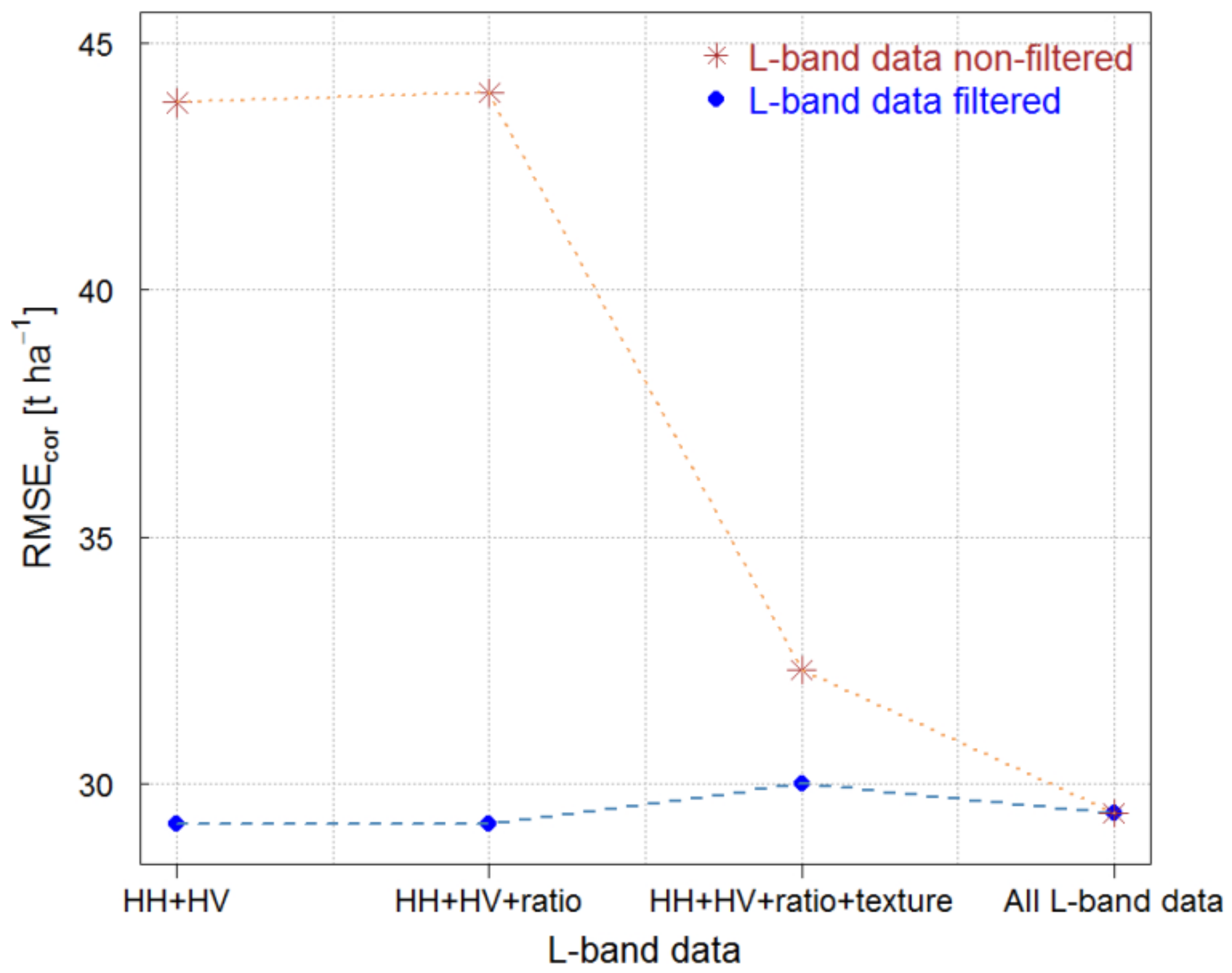
• examine the merit of the additional measures from the SAR backscatter for AGB retrieval.

2. Study Area and Data

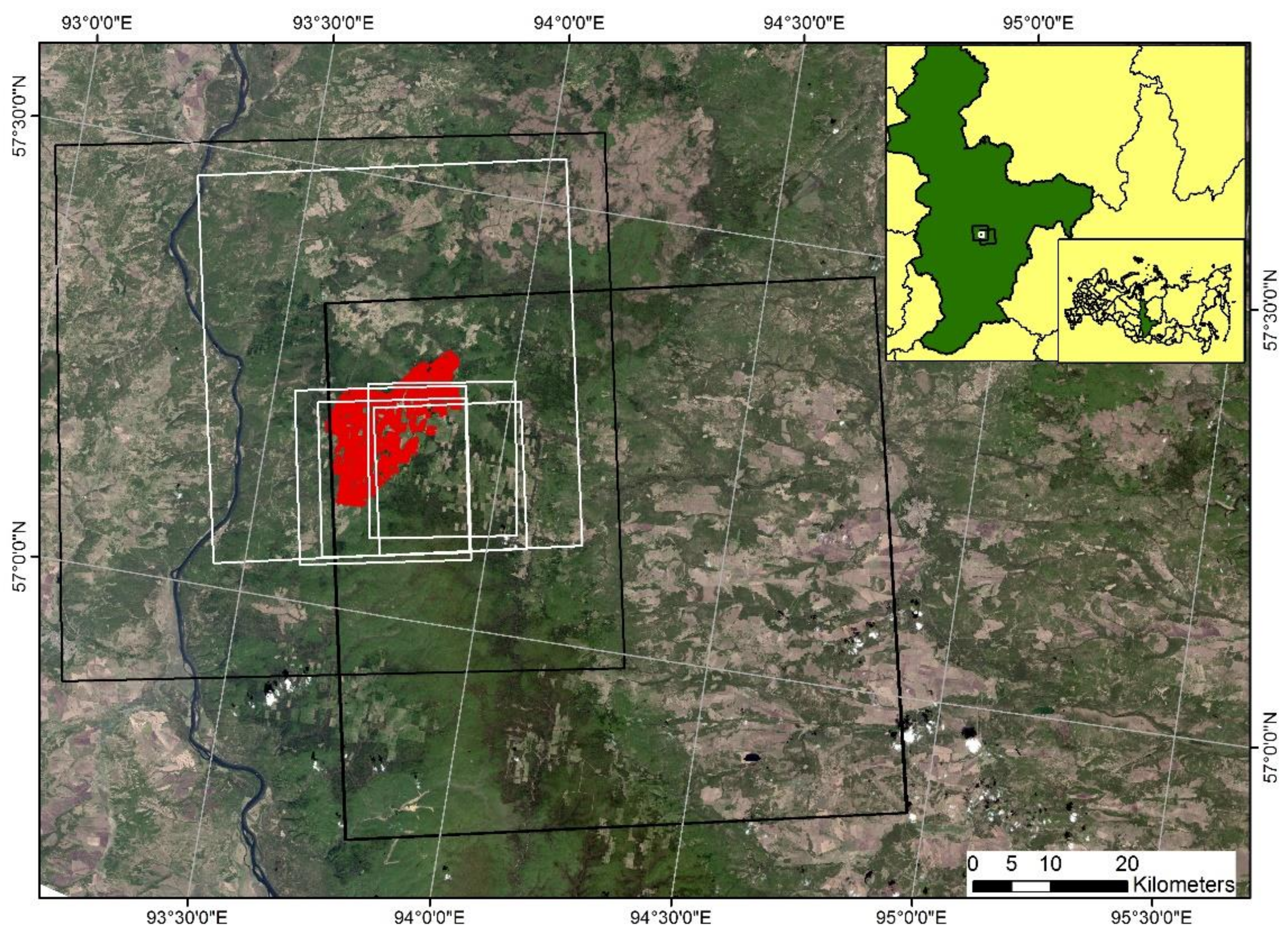
2.1. Study Area

Siberia is a vast region in Russia that accounts for more than three-quarters of the country’s land. The region is divided into three main parts: Western, Central and Eastern Siberia. In this study, a research area located in the southern part of Central Siberia was investigated for AGB estimation (Figure 1). The study area belongs to the Bolshe Murtinsky forest enterprise, located in the boreal forest ecosystem with a total carbon density (tree stems + branches + roots + foliage) of more than 6 kg C m⁻² [6]. Forests in the area of interest are dense and partially managed with dynamic logging activities. They are characterized by a continental climate with long, severe winters and short, warm, and wet summers. From mid-October until the beginning of April, the mean temperature is approximately −15 °C, while in summer the mean temperature is approximately +15 °C. The annual precipitation is below 450 millimetres. The dominant tree species are Fir (Abies sibirica), Birch (Betula pendula, Betula pubescens), Aspen (Populus tremula), Siberian Pine (Pinus sibirica), Pine (Pinus sylvestris), Spruce (Picea obovota) and Larch (Larix sibirica, Larix dahurica). In terms of topography, the study area has a gentle relief with heights from 150 m above sea level (a.s.l.) up to 520 m a.s.l., with an average height of 280 m a.s.l. The slopes range from 0° to 36°, with a mean value of 8°. The research covered an area of more than 210 km² and consisted of overlapping remote sensing data along with updated inventory data.

2.2. Above-Ground Biomass Reference Data

AGB reference data were derived from the growing stock volume (GSV) values collected and reported in the State Forest Account [65]. The forest inventory consisted of a polygon layer and the associated attribute table. For each forest stand, i.e., homogenous area in terms of forest structure and composition as well as geology, the following information was available: land category, density, age of dominant species, mean height, mean diameter at 1.3 meters above ground (dbh), and GSV calculated from these measurements. This inventory dated back to 1998. Because of the gap of 16 years between the inventory and the SAR data acquisitions, the field data were updated to = 2014 (see Section 3.1 for more details). The resulting AGB values are presented in the histogram (Figure 2) and ranged from 0 (non-forest) to 211 t ha⁻¹, with a mean value of 94 t ha⁻¹. The forest stand size varied from 3 ha to 127 ha, with a mean value of 18.5 ha. The stand age varied from 0 years to 292 years. In total, 494 forest stands were available for the investigation.

2.3. SAR Data

Data from two SAR satellites were used: Data from the L-band radar of the Phased Array Type L-band Synthetic Aperture Radar 2 (PALSAR-2) aboard the Advanced Land Observing Satellite (ALOS-2) of the Japan Aerospace Exploration Agency (JAXA) were combined with the C-band data from the RADARSAT-2 satellite of the Canadian Space Agency (CSA). The ALOS-2 PALSAR-2 data were available within the Kyoto and Carbon Initiative [66], whereas the RADARSAT-2 data were provided by the European Space Agency and CSA within the Second Call of the Sciences and Operational Application Research over Europe and Canada (SOAR-2). The ALOS-2 PALSAR-2 is an active sensor that has been in operation since 2014. It acquires SAR data from the sun-synchronous orbit (mean altitude 628 km) with a 14-day revisit time. The RADARSAT-2 mission has been active since 2007 and acquires data from the sun-synchronous polar orbit (mean altitude 798 km) with a 24-day revisit time. Both data sources were used to estimate AGB for the study area for the year 2014.

The data were acquired in single (horizontal transmitted, horizontal received, HH) and dual (HH and horizontal transmitted, vertical received, HV) polarizations in single look complex format (SLC). The ALOS-2 PALSAR-2 data were acquired in stripmap fine observation mode and the RADARSAT-2 data in ultrafine and fine mode. In total, four ALOS-2 PALSAR-2 and seven RADARSAT-2 images were available for this study (see

Table 1. Summary of SAR data available for the study area.

Satellite	Scene/Product ID	Image Name	Acquisition Time (YYYY/MM/DD; HH:MM UTC)	Observation Mode (Polarization)	Incidence Angle [°]/Ground Range; Azimuth [m]
ALOS-2 PALSAR-2	ALOS2018571143-140926	PSAR2_20140926_HH PSAR2_20140926_HV	2014/09/26; 17:16	Fine Dual (HH, HV)	31.4/ 4.3; 3.2
	ALOS2019311140-141001	PSAR2_20141001_HH PSAR2_20141001_HV	2014/10/01; 17:23	Fine Dual (HH, HV)	36.3/ 4.3; 3.7
RADARSAT-2	PDS_03827460	RSAT2_20140625_HV	2014/06/25; 11:21	Ultrafine (HV)	32.2/ 2.5; 2.1
	PDS_03827470	RSAT2_20140719_HH RSAT2_20140719_HV	2014/07/19; 19:21	Fine (HH, HV)	32.0/ 8.9; 4.8
	PDS_03932440	RSAT2_20140729_HV	2014/07/29;11:30	Ultrafine (HV)	39.2/ 2.1; 2.1
	PDS_03932470	RSAT2_20140805_HH	2014/08/05; 11:25	Ultrafine (HH)	35.4/ 2.3; 2.1
	PDS_04058330	RSAT2_20141002_HH RSAT2_20141002_HV	2014/10/02; 11:34	Fine (HH, HV)	42.1/ 7.1; 4.7

for summary).

The comparison of the C- and L-band data acquired in different image modes can be seen in Figure 3. Based on these examples, the influence of the radar frequency can be observed. The influence of the incidence angle can be ignored, as it is similar for all presented examples. The radiation from the C-band sensor penetrates only small objects, such as tree leaves on top of the tree canopy, that equal the wavelength, λ = 5.5 cm. On the other hand, data acquired with the L-band (λ = 23.8 cm) radar enables deeper imaging depth providing information related to branches and eventually tree trunks.

Both HH and HV polarizations were applied for above-ground biomass (AGB) estimation. Due to the lack of data acquired under frozen stable conditions, calculation of the InSAR coherence was not considered in this study.

The digital elevation model (DEM) from the Shuttle Radar Topography Mission (SRTM) version 4.1 [67,68] was used to pre-process the SAR data; i.e., for terrain correction and geocoding.

2.4. Weather Data

Since the penetration depth of the electromagnetic wave in an object is inversely proportional to its dielectric properties (water content), information about the weather conditions during the acquisition time were recorded. The corresponding weather conditions during data acquisition were available from the Kazachinskoye weather station, collected from http://www.sibessc.uni-jena.de/ (

Table 2. Weather conditions during SAR data acquisition. (Data source: NOAA National Climatic Data Center).

Image Name	Weather Conditions (Temperature Temp. in °C; mean wind speed WDSP in m s−1; Precipitation PRCP in mm)
PSAR_20140926_HH PSAR_20140926_HV	Temp. −1.3 °C; WDSP 1.2; PRCP 0
PSAR2_20141001_HH PSAR2_20141001_HV	Temp. 7.7 °C; WDSP 1.1; PRCP 0
RSAT2_20140625_HV	Temp. 22.2 °C; WDSP 1.6; PRCP 0
RSAT2_20140719_HH RSAT2_20140719_HV	Temp. 17.4 °C; WDSP 1.9; PRCP 0.5
RSAT2_20140729_HV	Temp. 17.8 °C; WDSP 1.9; PRCP 3
RSAT2_20140805_HH	Temp. 19.9 °C; WDSP 1; PRCP 0; 4 days before high PRCP
RSAT2_20141002_HH RSAT2_20141002_HV	Temp. 8.6 °C; WDSP 1.2; PRCP 0

). The weather parameters are given as a mean from eight daily measurements.

3. Methods

3.1. Above-Ground Biomass Data

For updating the available forest inventory data, the semi-empirical phytomass models and growth (i.e., yield) tables that were developed by the International Institute for Applied Systems Analyses (IIASA) in collaboration with V.N. Sukachev Institute of Forests, Siberian Branch, Russian Academy of Sciences, and Moscow State Forest University, were used [69,70]. The implementation of the models and tables in forestry and forest management in Russia has been recommended by the Council of the Federal Agency of Forest Management (Protocol No 2 dated 8 June 2006). The yield models satisfactorily, i.e., root-sum-square difference did not exceed ±3%, represented growth of Northern Eurasia’s boreal forests [70]. The improvement of the old inventory data was done using the information about mean tree height and mean age of a stand. In the first step, the site index (SI) of a forest stand was calculated. SI is defined as the edaphic and climatic characteristics of a site which have an impact on the growth and yield of a given tree species [4]. Next, the growth rate was derived by implementing the growth function. The new GSV was calculated as a sum of the GSV measured in the field and the GSV growth derived for an age difference between the available forest inventory and the reference year 2010. In the final step, the GSV was converted to AGB using a regional allometric model. The model was developed using freely available in situ measurements of forest live biomass (phytomass) [71]. Details about the insitu data update and conversion from the GSV into the AGB are given in Reference [23]. Additionally, the forest stands with logging areas after 2010 were removed by means of visual interpretation against the SAR data available for this study. The forest stands were buffered by 2 pixels, and the updated forest inventory database was used for AGB model calibration and validation. In total, 349 polygons were used for further analysis.

3.2. SAR Data Processing and Analysis

First, the SAR data were calibrated and multi-looked. The multi-looking factor (MLI) in the case of the ALOS-2 PALSAR-2 data was 2 × 4 and 2 × 5 in range and azimuth, for an image acquired in September and in October, respectively. The resulting resolution was approximately 15 m. Similarly, the RADARSAT-2 data were multi-looked with the MLI 5 × 5 and 2 × 4 in range and azimuth in the case of the ultrafine and fine acquisition modes, respectively. This produced a spatial resolution of 15 m and 20 m. Next, the backscattering coefficient γ⁰ was calculated in dB which includes a correction taking into account the local incidence angle [72].

Additionally, the ratio between the polarizations HH and HV was calculated. It was observed that integration of the ratios improves the estimation of AGB by increasing the saturation level [13,14,47]. Furthermore, ratios can reduce errors resulting from topography [73,74,75] and forest structure [13,14].

In order to decrease the speckle effect in the images, the enhanced Lee filter [76] was used. The filter uses local statistics (coefficient of variation), reducing speckle and at the same time preserving texture information in the radar data. In the case of homogenous areas, the pixel value is replaced by the average of the filter window; in the case of heterogeneous areas, the pixel value is replaced by a weighted average; and in the case of point objects, the pixel value is not changed. This filter outperformed other speckle filtering methods [77]. A window size of 5 × 5 and 3 × 3 was used for ALOS-2 PALSAR-2 and RADARSAT-2 data, respectively. As a result of filtering, the equivalent number of looks (ENL) of the images increased from two to three times. The ENL was estimated from the image statistics for a homogenous region, where the backscatter coefficient is assumed to be constant.

Additionally, texture measures were calculated to produce additional features by making use of spatial variations within the image. The gray level co-occurrence matrix (GLCM) proposed by Haralick et al. [78] is one of the most widely used methods to compute second-order texture measures. The measures were calculated as a probability of the occurrence of two gray levels separated by a given distance in a given direction. The texture measures were performed using data without speckle filtering because filtering reduces texture characteristics. The texture measures showed potential for biomass estimation [79]. The following measures were computed: sum average (mean), variance, homogeneity, contrast, dissimilarity, entropy, second moment, and correlation. For AGB estimation, the sum average co-occurrence matrix was selected by means of visual interpretation.

Altogether, forty-five SAR products were generated, out of which eighteen were from the ALOS-2 PALSAR-2 and twenty-seven were from the RADARSAT-2 data. The SAR products were resampled to a resolution of 50 m (0.25 ha) using the nearest neighbor method.

3.3. Above-Ground Biomass Retrieval

The SAR data and the forest inventory data were used as inputs for a non-parametric data fusion machine learning algorithm, random forests (RF) [80]. The workflow used for AGB estimation is shown graphically in Figure 4. The RF algorithm is widely used in ecology [81,82,83] as well as in forestry research [84,85,86]. Recent studies [87,88] have shown that RF is superior to other methods such as support vector machine (SVM), back propagation neural networks (BPNN), k-nearest neighbor (KNN), Gaussian processes (GP), and step-wise linear models (SLM).

RF is an ensemble learning method, which operates by combining random decision trees with bootstrap aggregation (bagging). The predictors are aggregated using bootstrap samples from training sets, and it has been shown that this method produces more accurate resultant predictors than the original predictor [89].

In general, five models using the regression mode of RF were constructed. The models consisted of: L-band data (Model 1); C-band data acquired in two modes ultrafine and fine (Model 2); C-band data in ultrafine mode (Model 3); C-band data in fine mode (Model 4); and L- and C-band data combined (Model 5).

In addition to bagging, the models were resampled during the model tuning using 10-fold cross-validation. Two thousand samples were used per AGB class for model calibration. The sample points within the AGB class were randomly distributed.

3.4. Unbiased Validation

An independent validation was performed using approximately 30% of the forest inventory data (117 forest stands). The prediction models were evaluated using the following four quantitative measures:

• corrected root mean squared error, defined as:

  $$RMS{E}_{cor}=\sqrt{RMS{E}_{Sat}^2-RMS{E}_{Ref}^2},$$

  (1)

  where $RMS{E}_{Sat}$ represents the root mean squared error in satellite-derived estimation of AGB and $RMS{E}_{Ref}$ is the root mean square error in forest inventory data. According to the manual on forest inventory and planning in Russian forests, the maximum error of RMSE_Ref is expected to be 15% [90].
• corrected relative root-mean-square error, defined as:

  $$relRMS{E}_{cor}=\frac{RMS{E}_{cor}}{{\overline{AGB}}_{Ref}}$$

  (2)

  shows that $RMS{E}_{cor}$ is divided by the mean of reference AGB.
• bias of the mean estimation error, defined as:

  $$bias=\frac{{{\displaystyle \sum }}_{i=1}^n\left( {\widehat{AGB}}_i-AG{B}_{ref\left(i\right)}\right)}{n}$$

  (3)

  represents $AG{B}_{ref\left(i\right)}$ as AGB reference value for stand i, $\widehat{AG{B}_i}$ as predicted AGB, and n as the number of AGB observations. Positive values of bias express overestimation, and vice versa.
• coefficient of determination, shown as:

  $$R^2=1-\frac{S{S}_{res}}{S{S}_{tot}},$$

  (4)

  where $S{S}_{res}$ is the sum of squares of the residuals and $S{S}_{tot}$ represents the total sum of squares.

The validation was performed using 1000 randomly distributed samples per AGB class.

4. Results

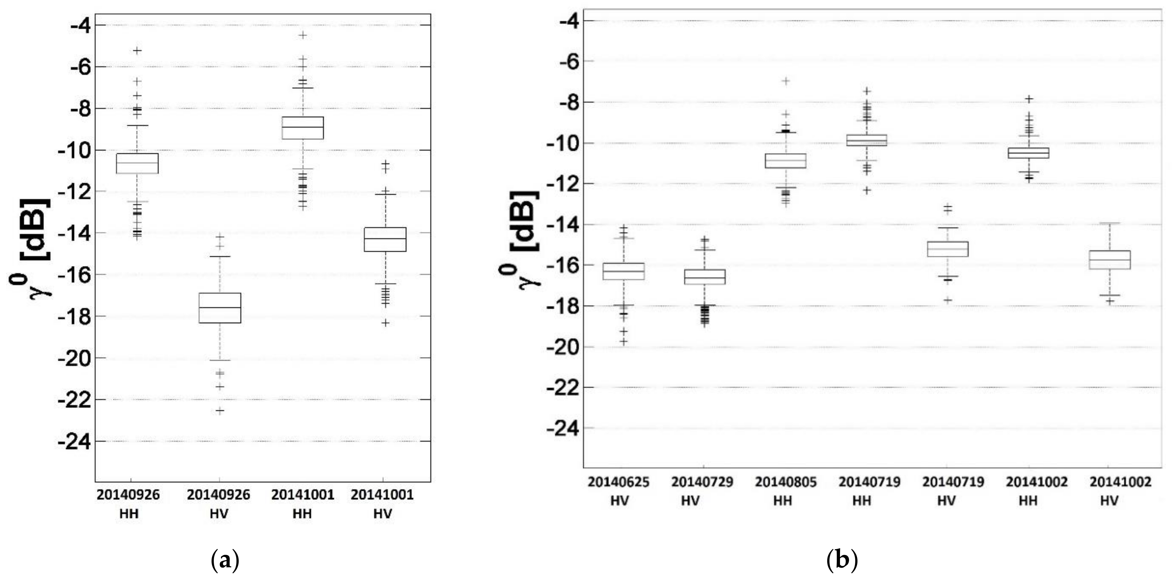
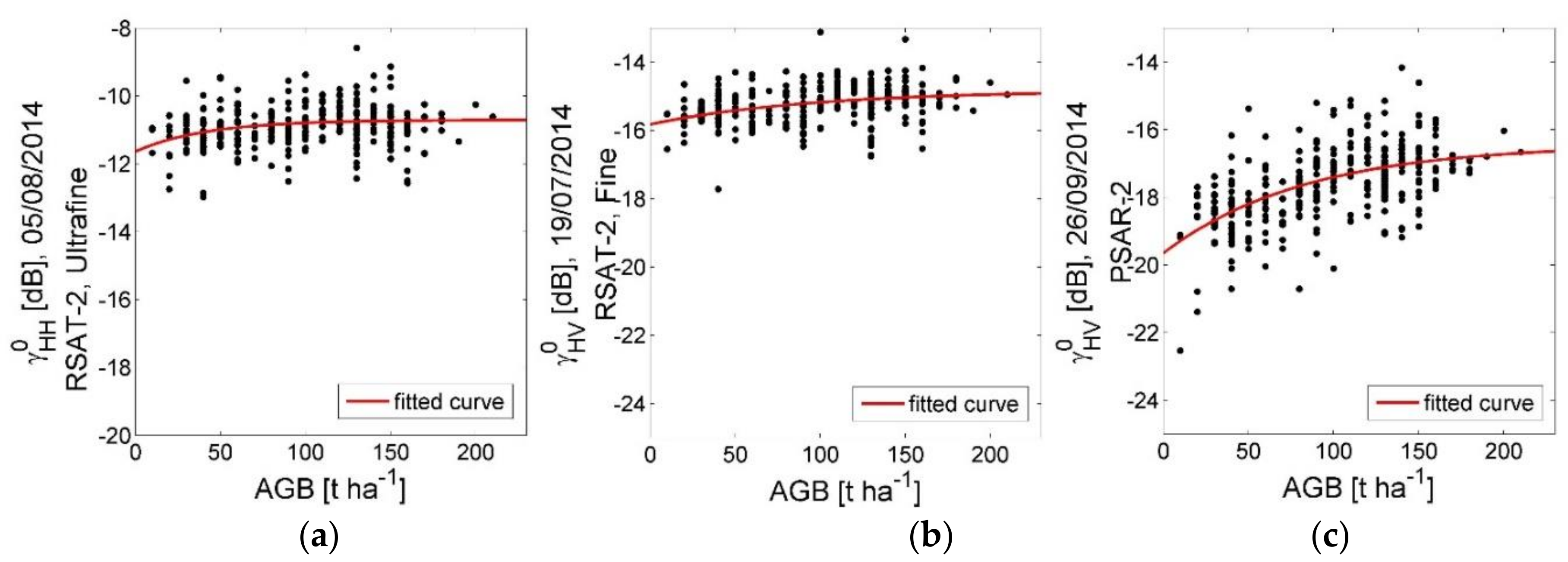
4.1. SAR Data Analysis

The results of the SAR data analysis are presented in Figure 5 and Figure 6. The boxplots show the backscattering coefficient statistics for available forest stands: the minimum (the horizontal line at the bottom of each plot), the median (50th percentile), the 25th and 75th percentile (the lower and upper quartile, respectively), the SAR image maximum (the horizontal line at the top of each plot) as well as outliers. A dynamic range of 7 dB and 4 dB was observed for ALOS-2 PALSAR-2 and RADARSAT-2 data, respectively. We present three examples of the data acquired in fine and ultrafine mode to show the correlation of the SAR backscatter with the AGB. An exponential model was applied to express these relations as described in [29,37].

The following exponential model was applied:

$${\mathsf{\gamma }}^0\left(AGB\right)=a{e}^{-cAGB}+b(1-e^{-cAGB})$$

(5)

where a and b are unknown coefficients that can be derived from the training data; a represents backscatter from ground, b represents backscatter from forest, and c represents the empirical coefficient that depends on forest structure and dielectric properties of the canopy. For unfrozen conditions an approximation of 0.008 was found to be reasonable [91]. The model corresponds to the simplified version of the water cloud model by Attema and Ulaby [92]. As expected, the C-band data showed the well-known saturation effect earlier. No significant relations were observed between the C-band data and field-estimated AGB.

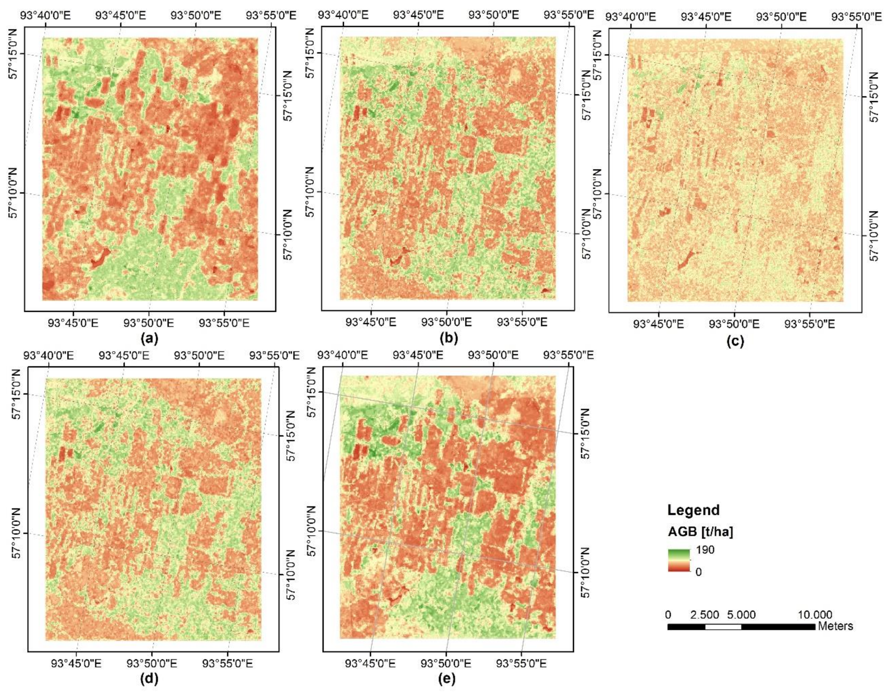
4.2. Above-Ground Biomass Maps

Figure 7 shows the resulting AGB maps with a pixel spacing of 50 m. The maps were derived using Models 1 to 5. The predicted results were expressed in t ha⁻¹. The statistics of the estimated AGB are given in

Table 3. Estimated AGB values for forest stands.

Model	Data	AGB Statistics [t ha−1]
		Min	Max	Mean
Model 1	PALSAR-2 18 products	8.8	166.7	89.5
Model 2	RADARSAT-2 27 products	14.8	166.5	89.5
Model 3	RADARSAT-2 Ultrafine 9 products	21.3	155	86.7
Model 4	RADARSAT-2 Fine 18 Products	21.7	161.4	89.7
Model 5	PALSAR-2 and RADARSAT-2 45 products	6.8	173.8	90.1

. When examining the results visually, differences could be observed among the maps in terms of the spatial variability of AGB values and the AGB value range. The AGB maps estimated from the C-band data acquired in ultrafine mode (Model 3) were characterized by the homogenous AGB values, whereas the AGB values estimated from the L-band (Model 1) and combined L- and C-band data (Model 5) showed the highest heterogeneity.

The AGB ranges from Model 1 (L-band data) and Model 5 (combination of L- and C-band data) corresponded most highly with the reference AGB values. This could be also observed on the scatterplots of estimated AGB displayed against the reference (Figure 8). All plots showed overestimation of AGB values < 80 t ha⁻¹ and underestimation > 80 t ha⁻¹. However, the AGB values estimated using the C-band data showed larger over and underestimation than the L-band based results.

It could be observed that the inclusion of the C-band data reduced the over and underestimation to some extent. The over and underestimation were partly caused by the ensemble (averaging) of regression trees, and partly by SAR saturation effects at high AGB ranges, and moisture and roughness effects at low AGB values.

The feature importance of the multi-looked backscattering coefficient calculated from C- and L-band data was presented and discussed in Reference [93]. The authors reported that the PALSAR-2 data acquired on 26/09/2014 in HV polarization were the most important for the retrieval of AGB, while the least important variable was the RADARSAT-2 data acquired on 19/07/2014 in fine mode, in HH polarization.

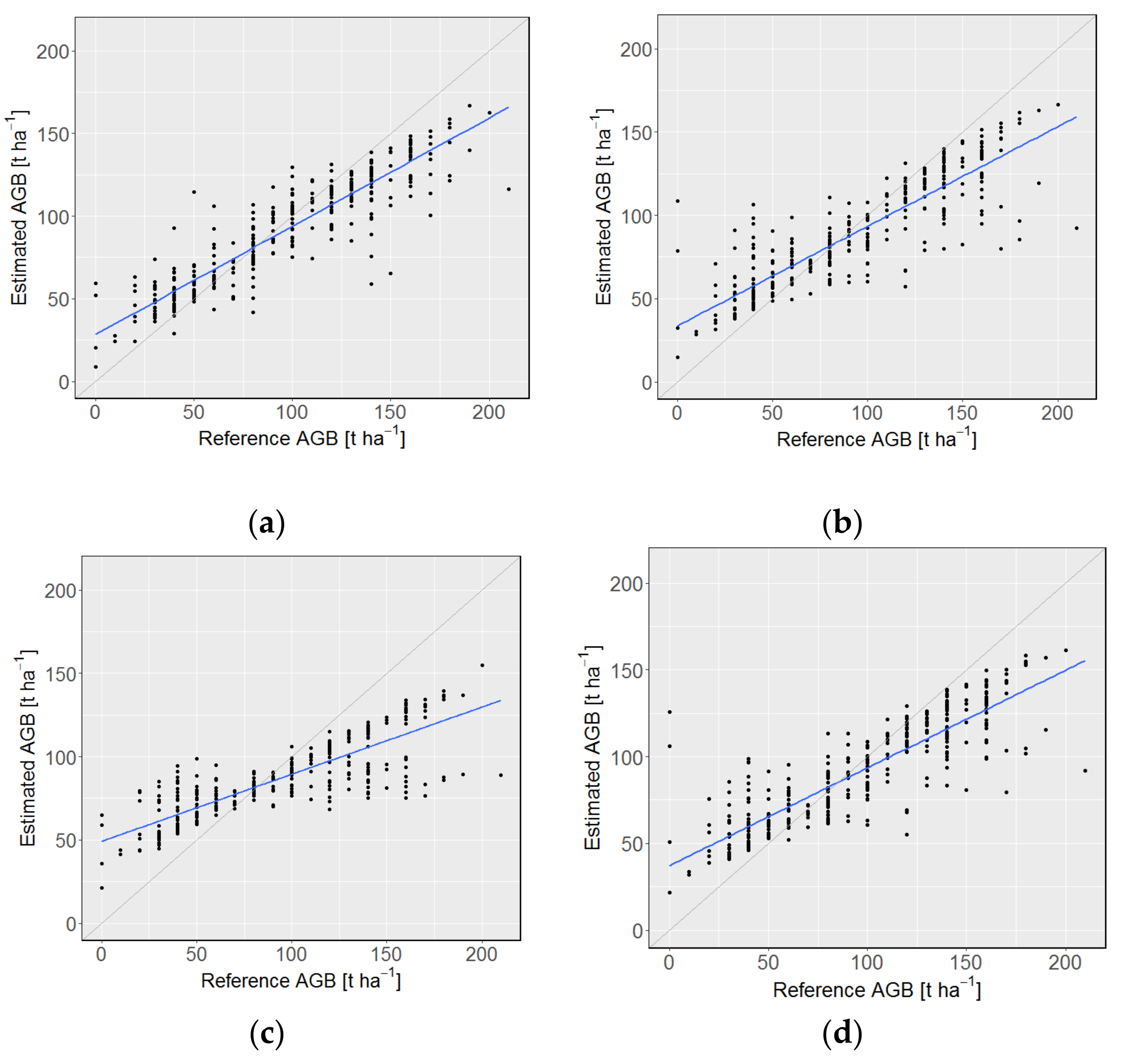
4.3. Unbiased Validation

Table 4. Validation statistics.

Model	Data	RMSEcor [t ha−1]	rel. RMSEcor	R2	Bias [t ha−1]
Model 1	PALSAR-2 18 products	29.4	0.31	0.53	5.5
Model 2	RADARSAT-2 27 products	39.5	0.42	0.23	5.6
Model 3	RADARSAT-2 Ultrafine 9 products	44.6	0.47	0.04	10.6
Model 4	RADARSAT-2 Fine 18 Products	41.1	0.44	0.17	3.9
Model 5	PALSAR-2 and RADARSAT-2 45 products	30.2	0.32	0.51	4.7

summarizes the validation results of the predicted AGB using the machine learning algorithm from the L-band ALOS-2 PALSAR-2 and C-band RADARSAT-2 backscatter data.

Additionally, a detailed investigation of the RMSE_cor in the case of the L-band data was performed (Figure 9). The comparison of the RMSE_cor has shown that it is sufficient to use the filtered L-band data in HH and HV polarization for the estimation of AGB. Inclusion of the ratio and texture measure in the retrieval slightly increased the AGB estimation error.

In general, the results obtained from L-Band data (Model 1) and combined L- and C-band data (Model 5) showed lower estimation errors. The RMSE_cor of 29.4 t ha⁻¹ (29.1 t ha⁻¹ in case of L-band filtered data used alone) and of 30.2 t ha⁻¹ (combination of L- and C-band backscatter intensities) were calculated, respectively. The highest RMSE_cor was derived when the C-band data alone were used; 44.6 t ha⁻¹ for C-band data acquired in ultrafine mode (Model 3), 41.1 t ha⁻¹ for C-band data acquired in fine mode (Model 4), and 39.5 t ha ⁻¹ for all available C-band data (Model 2). The coefficient of determination (R²) varied from 0.53 to 0.04 in the case of AGB estimations using Model 1 (L-band data) and that with Model 3 (C-band lutrafine mode). Overall, all models provided overestimated AGB values, with bias varying from 3.9 (C-band in fine mode) to 10.6 (C-band in ultrafine mode).

5. Discussion

Multi-frequency, multi-polarization, and multi-temporal data from L-band ALOS-2 PALSAR-2 and from C-band RADARSAT-2, together with updated in situ data were utilized for the first time to evaluate the improvement of above-ground biomass (AGB) estimation using a non-parametric biomass model. This allowed us to isolate the data source that provided the most information on forest biomass. Backscatter coefficients from L- and C-band radar were used independently, and in combination, to assess a boreal forest study area in, Siberia (Krasnoyarskiy Kray). Furthermore, the effects of including texture measures in AGB retrieval were investigated. The data from both SAR systems, as well as the additional generated SAR features, were combined in a machine learning algorithm (random forests).

As expected, the AGB modeling results indicated that the longer wavelength L-band data in HH and HV polarizations performed better than C-band data in HH and HV polarizations. This finding is in line with previous studies (e.g., References [25,44,62,93,94]). When the L-band data alone were used for the retrieval, a corrected relative root-mean-square error (RMSE_cor) of 29.4 t ha⁻¹ was calculated. The RMSE_cor decreased when only the filtered L-band backscatter data, without ratio and texture, were applied (29.1 t ha⁻¹). The ratio of backscatter was not found to be effective, similar to the research results reported in Reference [79]. The first multi-frequency approaches for boreal forests reported errors of 37.6 t ha⁻¹ [44] or 25.7 t ha⁻¹ [43] using the SIR-C/X-SAR data. It was shown that the L-band in HV polarization was the most important variable for AGB estimation [95], the same as in Reference [42]. Using the empirical parametric model (stepwise regression procedure) the L-band data in HV polarization were selected as the best information for biomass estimation for boreal forests, followed by the L-band in HH, L-band in VV, and C-band in HV polarization. Moreover, the ratio of HV backscatter from a longer wavelength to that from a shorter wavelength, as well as the ratio of texture measures, have been reported to provide good results for mapping the biomass [14,73,75,96]. The inclusion of the C-band data for AGB estimation only marginally improved the retrieval results. The over and underestimation was reduced, the bias decreased from 5.5 t ha⁻¹ to 4.7 t ha⁻¹, and the estimated AGB range corresponded to the reference data. However, the RMSE_cor increased by approximately 1% when calculated in combination with C-band and L-band data (30.2 t ha⁻¹) as opposed to when only using the latter (29.4 t ha⁻¹). In the case of African savannah a small improvement of 0.6 t ha⁻¹ was reported [53]. Moreover, the authors observed an improvement in the modeling estimations of the complete savannah vegetation structure. It is expected that integration of seasonal and/or annual time series of C-band acquisitions, i.e., from Sentinel-1, should improve the AGB retrieval. Hyper-temporal or multi-temporal (10 stacks of 3-month scenes) approaches using C-band data can provide accurate AGB estimations of approximately 15–20% RMSE, as reported in References [48,60].

The better performance in the first scenario, i.e., when only L-band data were used, was due to deeper wavelength penetration into the canopy, providing information from trunks and big branches that are better correlated with the forest AGB, especially in case of dense forests. The information from the C-band data comes mainly from tree leaves and small branches at the top of the canopy. Moreover, the RADARSAT-2 data acquired in the ultrafine mode showed more sensitivity to the roughness of the objects, decreasing the correlation between the SAR and the reference data, and thus generating higher estimation errors. This shows that the long wavelength SAR is better suited for the high forest biomass values and the short wavelength SAR for low biomass ranges. This finding also corresponds to recently reported results in the case of the African savannah test site [53], as well as tropical forests in Indonesia, where instead of C-band the X-band data were combined with L-band [49].

In general, the AGB estimation using L-band data alone, and in combination with C-band data was successful. However, it is important to mention the additional sources of error which were not taken into account in this study. The first source of error relates to the time difference between the SAR datasets and the insitu data, as well as the implementation of yield models. Even though the reference data have been updated using recommended growth models and include removal of the forest stands with extensive logging activities, it is very probable that local changes in the forest structure caused by smaller events, such as selective logging and local fires, were not taken into account. However, it was assumed that the main forest structure had not been changed. Different time and weather conditions resulting in different forest states during the SAR acquisitions could also influence the obtained AGB estimates.

AGB estimations in boreal forests using multi-frequency, multi-polarization and multi-temporal data are not very common. It is assumed that retrieval of AGB over boreal forests can be further improved by using texture ratio and multi-temporal InSAR coherence, and by implementing further SAR frequencies (X-band and P-band) in the analysis. The use of multi-frequency data should improve AGB estimation, as the biomass-related information in the SAR data acquired using different wavelengths comes from different forest compartments; i.e., trunks, branches, and foliage. Moreover, the inclusion of optical data can further reduce the estimation error, as this type of data provide important information on the deciduous/evergreen dominance [48]. Additionally, the use of a deep learning based workflow can increase the AGB accuracy as reported by Reference [88].

6. Conclusions

This study investigated the potential use of multi-frequency (C- and L-band), multi-polarization (HH and HV), and multi-temporal SAR data for AGB estimation in boreal forests. In total forty-five predictor layers were generated using RADARSAT-2 and ALOS-2 PALSAR-2 data, including texture measures.

The research showed that the inclusion of C-band data to the AGB non-parametric retrieval procedure marginally improved the estimation. It is assumed that the use of longer time series of the multi-frequency data will improve the AGB estimation, as the biomass-related information in the SAR data acquired using different wavelengths represents different tree parts and forest structures. The lowest estimation error RMSE_cor was calculated for L-band filtered data alone and was 29.1 t ha⁻¹ (rel RMSE_cor of 30%). In previous studies where mono-frequency or multi-frequency data were applied, relative estimation errors in the range of 30–40% for Siberian boreal forests were reported [e.g., References 7,23,57,61]. However, the lowest estimation error was obtained for coarse spatial resolutions (e.g., 1 km). This study showed that for local applications at a scale of 0.25 ha highly accurate AGB estimations can be obtained.

It is expected that AGB estimations could be further improved by including multi-temporal metrics, texture ratio, and InSAR coherence as predictor variables, as well as optical data. Moreover, the use of hyper-temporal C-band data with long wavelength SAR data can further reduce the over and underestimation that is presented when using e non-parametric, i.e., machine or deep learning, algorithms.

References

1. FAO. Terrestrial Essential Climate Variables. For Climate Change Assessment, Mitigation and Adaptation—BIOMASS; FAO: Rome, Italy, 2009. [Google Scholar]
2. Bojinski, S.; Verstraete, M.; Peterson, T.C.; Richter, C.; Simmons, A.; Zemp, M. The concept of essential climate variables in support of climate research, applications, and policy. Bull. Am. Meteorol. Soc. 2014, 95, 1431–1443. [Google Scholar] [CrossRef]
3. Thurner, M.; Beer, C.; Ciais, P.; Friend, A.D.; Ito, A.; Kleidon, A.; Lomas, M.R.; Quegan, S.; Rademacher, T.T.; Schaphoff, S.; et al. Evaluation of climate-related carbon turnover processes in global vegetation models for boreal and temperate forests. Glob. Chang. Biol. 2017, 23, 3076–3091. [Google Scholar] [CrossRef] [PubMed] [Green Version]
4. Van Laar, A.; Akca, A. Forest Mensuration: Chapter 8 Tree and Stand Biomass; von Gadow, K., Pukkala, T., Tome, M., Eds.; Springer: Dordrecht, The Netherlands, 2007; Volume 13, pp. 183–199. [Google Scholar]
5. FAO. Global Forest Resources Assessment 2015; FAO: Rome, Italy, 2015. [Google Scholar]
6. Thurner, M.; Beer, C.; Santoro, M.; Carvalhais, N.; Wutzler, T.; Schepaschenko, D.; Shvidenko, A.; Kompter, E.; Ahrens, B.; Levick, S.R.; et al. Carbon stock and density of northern boreal and temperate forests. Glob. Ecol. Biogeogr. 2014, 23, 297–310. [Google Scholar] [CrossRef]
7. Hüttich, C.; Korets, M.; Bartalev, S.; Zharko, V.; Schepaschenko, D.; Shvidenko, A.; Schmullius, C. Exploiting Growing Stock Volume Maps for Large Scale Forest Resource Assessment: Cross-Comparisons of ASAR- and PALSAR-Based GSV Estimates with Forest Inventory in Central Siberia. Forests 2014, 5, 1753–1776. [Google Scholar] [CrossRef] [Green Version]
8. FAO. The Russian Federation Forest Sector Outlook Study to 2030; FAO: Rome, Italy, 2012. [Google Scholar]
9. Stelmaszczuk-Górska, M.; Thiel, C.; Schmullius, C. Remote Sensing for Aboveground Biomass Estimation in Boreal Forests. In Earth Observation for Land and Emergency Monitoring..; Balzter, H., Ed.; John Wiley & Sons Ltd.: West Sussex, UK, 2017; pp. 33–55. [Google Scholar]
10. Ji, L.; Wylie, B.K.; Nossov, D.R.; Peterson, B.; Waldrop, M.P.; McFarland, J.W.; Rover, J.; Hollingsworth, T.N. Estimating aboveground biomass in interior Alaska with Landsat data and field measurements. Int. J. Appl. Earth Obs. Geoinf. 2012, 18, 451–461. [Google Scholar] [CrossRef]
11. Le Toan, T.; Beaudoin, A.; Riom, J.; Guyon, D. Relating forest biomass to SAR data. IEEE Trans. Geosci. Remote Sens. 1992, 30, 403–411. [Google Scholar] [CrossRef]
12. Beaudoin, A.; Le Toan, T.; Goze, S.; Nezry, E.; Lopes, A.; Mougin, E.; Hsu, C.C.; Han, H.C.; Kong, J.A.; Shin, R.T. Retrieval of forest biomass from SAR data. Int. J. Remote Sens. 1994, 15, 2777–2796. [Google Scholar] [CrossRef]
13. Dobson, M.C.; Ulaby, F.T.; Pierce, L.E.; Sharik, T.L.; Bergen, K.M.; Kellndorfer, J.; Kendra, J.R.; Li, E.; Lin, Y.C.; Nashashibi, A.; et al. Estimation of forest biophysical characteristics in Northern Michigan with SIR-C/X-SAR. IEEE Trans. Geosci. Remote Sens. 1995, 33, 877–895. [Google Scholar] [CrossRef]
14. Ranson, K.J.; Sun, G. Mapping biomass of a northern forest using multifrequency SAR data. IEEE Trans. Geosci. Remote Sens. 1994, 32, 388–396. [Google Scholar] [CrossRef]
15. Fransson, J.E.S.; WaLter, F.; Ulander, L.M.H. Estimation of forest parameters using CARABAS-II VHF SAR data. IEEE Trans. Geosci. Remote Sens. 2000, 38, 720–727. [Google Scholar] [CrossRef] [Green Version]
16. Rauste, Y. Multi-temporal JERS SAR data in boreal forest biomass mapping. Remote Sens. Environ. 2005, 97, 263–275. [Google Scholar] [CrossRef]
17. Soja, M.J.; Sandberg, G.; Ulander, L.M.H.; Member, S. Regression-based retrieval of boreal forest biomass in sloping terrain using P-band SAR backscatter intensity data. IEEE Trans. Geosci. Remote Sens. 2013, 51, 2646–2665. [Google Scholar] [CrossRef]
18. Soja, M.J.; Persson, H.J.; Ulander, L.M.H. Estimation of forest biomass from two-level model inversion of single-pass InSAR data. IEEE Int. Geosci. Remote Sens. Symp. 2015, 53, 3886–3889. [Google Scholar] [CrossRef]
19. Santoro, M.; Cartus, O.; Fransson, J.; Shvidenko, A.; McCallum, I.; Hall, R.; Beaudoin, A.; Beer, C.; Schmullius, C. Estimates of Forest Growing Stock Volume for Sweden, Central Siberia, and Québec Using Envisat Advanced Synthetic Aperture Radar Backscatter Data. Remote Sens. 2013, 5, 4503–4532. [Google Scholar] [CrossRef] [Green Version]
20. Askne, J.; Fransson, J.; Santoro, M.; Soja, M.; Ulander, L. Model-based biomass estimation of a hemi-boreal forest from multitemporal TanDEM-X acquisitions. Remote Sens. 2013, 5, 5574–5597. [Google Scholar] [CrossRef]
21. Karjalainen, M.; Kankare, V.; Vastaranta, M.; Holopainen, M.; Hyyppä, J. Prediction of plot-level forest variables using TerraSAR-X stereo SAR data. Remote Sens. Environ. 2012, 117, 338–347. [Google Scholar] [CrossRef]
22. Wilhelm, S.; Hüttich, C.; Korets, M.; Schmullius, C. Large area mapping of boreal Growing Stock Volume on an annual and multi-temporal level using PALSAR L-band backscatter mosaics. Forests 2014, 5, 1999–2015. [Google Scholar] [CrossRef]
23. Stelmaszczuk-Górska, M.; Rodriguez-Veiga, P.; Ackermann, N.; Thiel, C.; Balzter, H.; Schmullius, C. Non-Parametric Retrieval of Aboveground Biomass in Siberian Boreal Forests with ALOS PALSAR Interferometric Coherence and Backscatter Intensity. J. Imaging 2016, 2, 24. [Google Scholar] [CrossRef]
24. Pulliainen, J.T.; Heiska, K.; Hyyppa, J.; Hallikainen, M.T. Backscattering properties of boreal forests at the C- and X-bands. IEEE Trans. Geosci. Remote Sens. 1994, 32, 1041–1050. [Google Scholar] [CrossRef]
25. Fransson, J.E.S.; Israelsson, H. Estimation of stem volume in boreal forests using ERS-1 C- and JERS-1 L- band SAR data. Int. J. Remote Sens. 1999, 20, 123–137. [Google Scholar] [CrossRef]
26. Antropov, O.; Rauste, Y.; Ahola, H.; Häme, T. Stand-level stem volume of boreal forests from spaceborne SAR imagery at L-band. IEEE Trans. Geosci. Remote Sens. 2013, 6, 4776–4779. [Google Scholar] [CrossRef]
27. Solberg, S.; Astrup, R.; Gobakken, T.; Næsset, E.; Weydahl, D.J. Estimating spruce and pine biomass with interferometric X-band SAR. Remote Sens. Environ. 2010, 114, 2353–2360. [Google Scholar] [CrossRef]
28. Koskinen, J.T.; Pulliainen, J.T.; Hyyppä, J.M.; Engdahl, M.E.; Hallikainen, M.T. The seasonal behavior of interferometric coherence in boreal forest. IEEE Trans. Geosci. Remote Sens. 2001, 39, 820–829. [Google Scholar] [CrossRef]
29. Santoro, M.; Askne, J.; Smith, G.; Fransson, J.E.S. Stem volume retrieval in boreal forests from ERS-1/2 interferometry. Remote Sens. Environ. 2002, 81, 19–35. [Google Scholar] [CrossRef]
30. Næsset, E.; Bollandsås, O.M.; Gobakken, T.; Solberg, S.; McRoberts, R.E. The effects of field plot size on model-assisted estimation of aboveground biomass change using multitemporal interferometric SAR and airborne laser scanning data. Remote Sens. Environ. 2015, 168, 252–264. [Google Scholar] [CrossRef]
31. Papathanassiou, K.P.; Cloude, S.R. Single-baseline polarimetric SAR interferometry. IEEE Trans. Geosci. Remote Sens. 2001, 39, 2352–2363. [Google Scholar] [CrossRef]
32. Neumann, M.; Saatchi, S.S.; Ulander, L.M.H.; Fransson, J.E.S. Assessing performance of L- and P-Band polarimetric interferometric SAR data in estimating boreal forest above-ground biomass. IEEE Trans. Geosci. Remote Sens. 2012, 50, 714–726. [Google Scholar] [CrossRef]
33. Antropov, O.; Rauste, Y.; Häme, T.; Praks, J. Polarimetric ALOS PALSAR Time Series in Mapping Biomass of Boreal Forests. Remote Sens. 2017, 9, 999. [Google Scholar] [CrossRef]
34. Tebaldini, S.; Rocca, F. Multibaseline polarimetric SAR tomography of a boreal forest at P- and L-bands. IEEE Trans. Geosci. Remote Sens. 2012, 50, 232–246. [Google Scholar] [CrossRef]
35. Persson, H.; Fransson, J. Forest variable estimation using radargrammetric processing of TerraSAR-X images in boreal forests. Remote Sens. 2014, 6, 2084–2107. [Google Scholar] [CrossRef]
36. Vastaranta, M.; Niemi, M.; Karjalainen, M.; Peuhkurinen, J.; Kankare, V.; Hyyppä, J.; Holopainen, M. Prediction of forest stand attributes using TerraSAR-X stereo imagery. Remote Sens. 2014, 6, 3227–3246. [Google Scholar] [CrossRef]
37. Santoro, M.; Eriksson, L.; Fransson, J. Reviewing ALOS PALSAR Backscatter Observations for Stem Volume Retrieval in Swedish Forest. Remote Sens. 2015, 7, 4290–4317. [Google Scholar] [CrossRef] [Green Version]
38. Eriksson, L.E.B. Satellite-borne L-band Interferometric Coherence for Forestry Applications in the Boreal Zone. Doctoral Thesis, University of Jena, Jena, Germany, 2004. [Google Scholar]
39. Le Toan, T.; Beaudoin, A.; Riom, J.; Guyon, D. Relating Forest Biomass to SAR Data. IEEE Trans. Geosci. Remote Sens. 1994, 30, 403–411. [Google Scholar] [CrossRef]
40. Rignot, E.; Way, J.; Williams, C.; Viereck, L. Radar estimates of aboveground biomass in boreal forests of interior Alaska. IEEE Trans. Geosci. Remote Sens. 1994, 32, 1117–1124. [Google Scholar] [CrossRef] [Green Version]
41. Saatchi, S.S.; Moghaddam, M. Estimation of crown and stem water content and biomass of boreal forest using polarimetric SAR imagery. IEEE Trans. Geosci. Remote Sens. 2000, 38, 697–709. [Google Scholar] [CrossRef] [Green Version]
42. Ranson, K.J.; Sun, G.; Lang, R.H.; Chauhan, N.S.; Cacciola, R.J.; Kilic, O. Mapping of boreal forest biomass from spaceborne synthetic aperture radar. J. Geophys. Res. 1997, 102, 29599–29610. [Google Scholar] [CrossRef] [Green Version]
43. Ranson, K.J.; Sun, G.; Member, S. Effects of Environmental Conditions on Boreal Forest Classification and Biomass Estimates with SAR. IEEE Geosci. Remote Sens. 2000, 38, 1242–1252. [Google Scholar] [CrossRef]
44. Ranson, K.J.; Sun, G.; Lang, R.H.; Chauhan, N.S.; Cacciola, R.J.; Kilic, O. An evaluation of AIRSAR and SIR-C/X-SAR images for mapping northern forest attributes in Maine, USA. Remote Sens. Environ. 1997, 59, 203–222. [Google Scholar] [CrossRef]
45. Wagner, W.; Luckman, A.; Vietmeier, J.; Tansey, K.; Balzter, H.; Schmullius, C.; Davidson, M.; Gaveau, D.; Gluck, M.; Le, T.; et al. Large-scale mapping of boreal forest in SIBERIA using ERS tandem coherence and JERS backscatter data. Remote Sens. Environ. 2003, 85, 125–144. [Google Scholar] [CrossRef] [Green Version]
46. Tsui, O.W.; Coops, N.C.; Wulder, M.A.; Marshall, P.L.; McCardle, A. Using multi-frequency radar and discrete-return LiDAR measurements to estimate above-ground biomass and biomass components in a coastal temperate forest. ISPRS J. Photogramm. Remote Sens. 2012, 69, 121–133. [Google Scholar] [CrossRef]
47. Harrell, P.A.; Kasischke, E.S.; Bourgeau-Chavez, L.L.; Haney, E.M.; Christensen, N.L. Evaluation of approaches to estimating aboveground biomass in Southern pine forests using SIR-C data. Remote Sens. Environ. 1997, 59, 223–233. [Google Scholar] [CrossRef]
48. Laurin, G.V.; Balling, J.; Corona, P.; Mattioli, W.; Papale, D.; Puletti, N.; Rizzo, M.; Truckenbrodt, J.; Urban, M. Above-ground biomass prediction by Sentinel-1 multitemporal data in central Italy with integration of ALOS2 and Sentinel-2 data. J. Appl. Remote Sens. 2018, 12, 18. [Google Scholar] [CrossRef]
49. Englhart, S.; Keuck, V.; Siegert, F. Aboveground biomass retrieval in tropical forests—The potential of combined X- and L-band SAR data use. Remote Sens. Environ. 2011, 115, 1260–1271. [Google Scholar] [CrossRef]
50. Englhart, S.; Member, S.; Keuck, V.; Siegert, F. Modeling Aboveground Biomass in Tropical Forests Using Multi-Frequency SAR Data—A Comparison of Methods. IEEE J. Sel. Top. Appl. Earth Obs. Remote Sens. 2012, 5, 298–306. [Google Scholar] [CrossRef]
51. Backscatter, P.R.; Neeff, T.; Dutra, L.V.; Freitas, C. Tropical Forest Measurement by Interferometric Height Modeling and P-Band Radar Backscatter. Biomass 2005, 51, 585–594. [Google Scholar]
52. Mougin, E.; Proisy, C.; Marty, G.; Fromard, F.; Puig, H.; Betoulle, J.L.; Rudant, J.P. Multifrequency and multipolarization radar backscattering from mangrove forests. IEEE Trans. Geosci. Remote Sens. 1999, 37, 94–102. [Google Scholar] [CrossRef]
53. Naidoo, L.; Mathieu, R.; Main, R.; Kleynhans, W.; Wessels, K.; Asner, G.; Leblon, B. Savannah woody structure modelling and mapping using multi-frequency (X-, C- and L-band) Synthetic Aperture Radar data. ISPRS J. Photogramm. Remote Sens. 2015, 105, 234–250. [Google Scholar] [CrossRef] [Green Version]
54. Askne, J.; Santoro, M.; Smith, G.; Fransson, J.E.S. Multitemporal repeat-rass SAR interferometry of boreal forests. IEEE Trans. Geosci. Remote Sens. 2003, 41, 1540–1550. [Google Scholar] [CrossRef]
55. Santoro, M.; Shvidenko, A.; Mccallum, I.; Askne, J.; Schmullius, C. Properties of ERS-1/2 coherence in the Siberian boreal forest and implications for stem volume retrieval. Remote Sens. Environ. 2007, 106, 154–172. [Google Scholar] [CrossRef]
56. Peregon, A.; Yamagata, Y. The use of ALOS/PALSAR backscatter to estimate above-ground forest biomass: A case study in Western Siberia. Remote Sens. Environ. 2013, 137, 139–146. [Google Scholar] [CrossRef]
57. Chowdhury, T.A.; Thiel, C.; Schmullius, C. Growing stock volume estimation from L-band ALOS PALSAR polarimetric coherence in Siberian forest. Remote Sens. Environ. 2014, 155, 129–144. [Google Scholar] [CrossRef]
58. Rodriguez-Veiga, P.; Stelmaszczuk-Górska, M.; Hüttich, C.; Schmullius, C.; Tansey, K.; Balzter, H. Aboveground Biomass Mapping in Krasnoyarsk Kray (Central Siberia) using Allometry, Landsat, and ALOS PALSAR. In Proceedings of the RSPSoc Annual Conference, Aberystwyth, UK, 15 June 2014. [Google Scholar]
59. Santoro, M.; Eriksson, L.; Askne, J.; Schmullius, C. Assessment of stand-wise stem volume retrieval in boreal forest from JERS-1 L-band SAR backscatter. Int. J. Remote Sens. 2006, 27, 3425–3454. [Google Scholar] [CrossRef]
60. Santoro, M.; Beer, C.; Cartus, O.; Schmullius, C.; Shvidenko, A.; McCallum, I.; Wegmüller, U.; Wiesmann, A. Retrieval of growing stock volume in boreal forest using hyper-temporal series of Envisat ASAR ScanSAR backscatter measurements. Remote Sens. Environ. 2011, 115, 490–507. [Google Scholar] [CrossRef]
61. Thiel, C.; Schmullius, C. The potential of ALOS PALSAR backscatter and InSAR coherence for forest growing stock volume estimation in Central Siberia. Remote Sens. Environ. 2016, 173, 258–273. [Google Scholar] [CrossRef]
62. Kurvonen, L.; Pulliainen, J.; Hallikainen, M. Retrieval of biomass in boreal forests from multitemporal ERS-1 and JERS-1 SAR images. IEEE Trans. Geosci. Remote Sens. 1999, 37, 198–205. [Google Scholar] [CrossRef]
63. Eriksson, L.E.B.; Santoro, M.; Wiesmann, A.; Schmullius, C.C. Multitemporal JERS repeat-pass coherence for growing-stock volume estimation of Siberian forest. IEEE Trans. Geosci. Remote Sens. 2003, 41, 1561–1570. [Google Scholar] [CrossRef]
64. Santoro, M.; Cartus, O. Research pathways of forest above-ground biomass estimation based on SAR backscatter and interferometric SAR observations. Remote Sens. 2018, 10, 608. [Google Scholar] [CrossRef]
65. Schmullius, C.; Baker, J.; Balzter, H.; Davidson, M.; Eriksson, L.; Gaveau, D.; Gluck, M.; Holz, A.; Le Toan, T.; Luckman, A.; et al. SAR Imaging for Boreal Ecology and Radar Interferometry Applications SIBERIA Project (Contract No. ENV4-CT97-0743-SIBERIA)—Final Report; Microwaves and Radar Institute: Jena, Germany, 2001. [Google Scholar]
66. Rosenqvist, Å.; Milne, A.; Lucas, R.; Imhoff, M.; Dobson, C. A review of remote sensing technology in support of the Kyoto Protocol. Environ. Sci. Policy 2003, 6, 441–455. [Google Scholar] [CrossRef]
67. CGIAR CSI. Available online: http://srtm.csi.cgiar.org (accessed on 15 April 2014).
68. Reuter, H.I.; Nelson, A.; Jarvis, A. An evaluation of void filling interpolation methods for SRTM data. Int. J. Geogr. Inf. Sci. 2007, 21, 983–1008. [Google Scholar] [CrossRef]
69. Shvidenko, A.; Schepaschenko, D.; Nilsson, S.; Bouloui, Y. Semi-empirical models for assessing biological productivity of Northern Eurasian forests. Ecol. Modell. 2007, 204, 163–179. [Google Scholar] [CrossRef]
70. Shvidenko, A.; Schepaschenko, D.; Nilsson, S.; Boului, Y. Tables and Models of Growth and Productivity of Forests of Major Forming Species of Northern Eurasia (Standard and Reference Materials); Federal Agency of Forest Management: Moscow, Russia, 2008. [Google Scholar]
71. IIASA Russian Forests & Forestry. Live Biomass & Net Primary Production—Measurements of Forest Phytomass in Situ. Available online: http://webarchive.iiasa.ac.at/Research/FOR/forest_cdrom/english/for_prod_en.html (accessed on 10 January 2014).
72. Ulander, L.M.H. Radiometrie slope correction of synthetic-aperture radar images. IEEE Trans. Geosci. Remote Sens. 1996, 34, 1115–1122. [Google Scholar] [CrossRef]
73. Ranson, K.J.; Saatchi, S.S.; Sun, G. Boreal Forest Ecosystem Characterization with SIR-C / XSAR. IEEE Trans. Geosci. Remote Sens. 1995, 33, 867–876. [Google Scholar] [CrossRef]
74. Soja, M.J.; Sandberg, G.; Ulander, L.M.H. Topographic correction for biomass retrieval from P-band SAR data in boreal forests. IEEE Int. Geosci. Remote Sens. Symp. 2010, 4776–4779. [Google Scholar] [CrossRef]
75. Ranson, K.J.; Sun, G.; Kharuk, V.I.; Kovacs, K. Characteristics of Forests in Western Sayani Mountains, Siberia from SAR Data. Remote Sens. Environ. 2001, 75, 188–200. [Google Scholar] [CrossRef]
76. Lopes, A.; Touzi, R.; Nezry, E. Adaptive Speckle Filters and Scene Heterogeneity. IEEE Trans. Geosci. Remote Sens. 1990, 28, 992–1000. [Google Scholar] [CrossRef]
77. Joshi, N.; Mitchard, E.; Schumacher, J.; Johannsen, V.; Saatchi, S.; Fensholt, R. L-band SAR backscatter related to forest cover, height and aboveground biomass at multiple spatial scales across Denmark. Remote Sens. 2015, 7, 4442–4472. [Google Scholar] [CrossRef]
78. Haralick, R.M.; Shanmugam, K.; Dinstein, I. Textural Features for Image Classification. IEEE Trans. Syst. Man. Cybern. 1973, SMC-3, 610–621. [Google Scholar] [CrossRef]
79. Sarker, M.L.R.; Nichol, J.; Ahmad, B.; Busu, I.; Rahman, A.A. Potential of texture measurements of two-date dual polarization PALSAR data for the improvement of forest biomass estimation. ISPRS J. Photogramm. Remote Sens. 2012, 69, 146–166. [Google Scholar] [CrossRef]
80. Breiman, L. Random Forests. Mach. Learn. 2001, 45, 5–32. [Google Scholar] [CrossRef] [Green Version]
81. Prasad, A.M.; Iverson, L.R.; Liaw, A. Newer classification and regression tree techniques: Bagging and random forests for ecological prediction. Ecosystems 2006, 9, 181–199. [Google Scholar] [CrossRef]
82. Hüttich, C.; Herold, M.; Strohbach, B.J.; Dech, S. Integrating in-situ, Landsat, and MODIS data for mapping in Southern African savannas: Experiences of LCCS-based land-cover mapping in the Kalahari in Namibia. Environ. Monit. Assess. 2011, 176, 531–547. [Google Scholar] [CrossRef] [PubMed]
83. Cutler, D.R.; Edwards, T.C.; Beard, K.H.; Cutler, A.; Hess, K.T.; Gibson, J.; Lawler, J.J. Random forests for classification in ecology. Ecology 2007, 88, 2783–2792. [Google Scholar] [CrossRef] [PubMed]
84. Cartus, O.; Kellndorfer, J.; Rombach, M.; Walker, W. Mapping Canopy Height and Growing Stock Volume Using Airborne Lidar, ALOS PALSAR and Landsat ETM+. Remote Sens. 2012, 4, 3320–3345. [Google Scholar] [CrossRef]
85. Cartus, O.; Kellndorfer, J.; Walker, W.; Franco, C.; Bishop, J.; Santos, L.; Fuentes, J. A National, Detailed Map of Forest Aboveground Carbon Stocks in Mexico. Remote Sens. 2014, 6, 5559–5588. [Google Scholar] [CrossRef] [Green Version]
86. Baccini, A.; Laporte, N.; Goetz, S.J.; Sun, M.; Dong, H. A first map of tropical Africa’s above-ground biomass derived from satellite imagery. Environ. Res. Lett. 2008, 3, 9. [Google Scholar] [CrossRef]
87. Fassnacht, F.E.; Hartig, F.; Latifi, H.; Berger, C.; Hernández, J.; Corvalán, P.; Koch, B. Importance of sample size, data type and prediction method for remote sensing-based estimations of aboveground forest biomass. Remote Sens. Environ. 2014, 154, 102–114. [Google Scholar] [CrossRef]
88. Shao, Z.; Zhang, L.; Wang, L. Stacked Sparse Autoencoder Modeling Using the Synergy of Airborne LiDAR and Satellite Optical and SAR Data to Map Forest Above-Ground Biomass. IEEE J. Sel. Top. Appl. Earth Obs. Remote Sens. 2017, 10, 5569–5582. [Google Scholar] [CrossRef]
89. Breiman, L. Bagging predictors. Mach. Learn. 1996, 24, 123–140. [Google Scholar] [CrossRef] [Green Version]
90. Federal Forestry Agency. Manual on Forest Inventory and Planning in Russian Forest; Federal Forestry Agency: Moscow, Russia, 1995. [Google Scholar]
91. Cartus, O.; Santoro, M.; Kellndorfer, J. Mapping forest aboveground biomass in the Northeastern United States with ALOS PALSAR dual-polarization L-band. Remote Sens. Environ. 2012, 124, 466–478. [Google Scholar] [CrossRef]
92. Attema, E.P.W.; Ulaby, F.T. Vegetation Modeled as a Water Cloud. Radio Sci. 1978, 13, 357–364. [Google Scholar] [CrossRef]
93. Harrell, P.A.; Bourgeau-Chavez, L.L.; Kasischke, E.S.; French, N.H.F.; Christensen, N.L., Jr. Sensitivity of ERS-1 and JERS-1 radar data to biomass and stand structure in Alaskan boreal forest. Remote Sens. Environ. 1995, 54, 247–260. [Google Scholar] [CrossRef]
94. Balzter, H.; Baker, J.R.; Hallikainen, M.; Tomppo, E. Retrieval of timber volume and snow water equivalent over a Finnish boreal forest from airborne polarimetric Synthetic Aperture Radar. Int. J. Remote Sens. 2002, 23, 3185–3208. [Google Scholar] [CrossRef] [Green Version]
95. Stelmaszczuk-Górska, M.; Thiel, C.; Schmullius, C. Retrieval of aboveground biomass using multi-frequency SAR. In Proceedings of the ESA Living Planet Symposium 2016, Prague, Czech Republic, 9–13 May 2016. [Google Scholar]
96. Sarker, L.R.; Nichol, J.; Iz, H.B.; Ahmad, B.; Rahman, A.A. Forest Biomass Estimation Using Texture Measurements of High-Resolution Dual-Polarization C-Band SAR Data. IEEE Trans. Geosci. Remote Sens. 2013, 51, 3371–3384. [Google Scholar] [CrossRef]
Figure 1. Location of the study area: footprints in black and white represent ALOS-2 PALSAR-2 and RADARSAT-2, respectively; the in situ measurements are presented in red. Landsat 5 Imagery acquired on 2 June 2007 is shown in the background. Landsat Image courtesy of the U.S. Geological Survey.
Remotesensing 10 01550 g001
Figure 2. Number of forest stands per above-ground biomass class.
Remotesensing 10 01550 g002
Figure 3. Multi-looked backscattering coefficient calculated for C- and L-band data: (a) optical image acquired by RapidEye on 11 June 2012; (b) C-band RADARSAT-2 image acquired in ultrafine mode on 5 August 2014; (c) C-band RADARSAT-2 image acquired in fine mode HH (on the left), HV (on the right) on 19 July 2014; (d) ALOS-2 PALSAR-2 image acquired in fine mode dual HH (on the left), HV (on the right) on 26 September 2014. The scale of images is 1:40,000.
Remotesensing 10 01550 g003
Figure 4. Above-ground biomass estimation processing steps.
Remotesensing 10 01550 g004
Figure 5. Backscattering coefficient statistics given for the data acquisition time (YYYYMMDD) and polarization (HH or HV): (a) ALOS-2 PALSAR-2 data; (b) RADARSAT-2 data.
Remotesensing 10 01550 g005
Figure 6. Synthetic Aperture Radar (SAR) backscatter as a function of forest above-ground biomass (AGB); red line represents exponential fit. Data from: (a) RADARSAT-2 ultrafine mode; (b) RADARSAT-2 fine mode; (c) ALOS-2 PALSAR-2 fine dual mode.
Remotesensing 10 01550 g006
Figure 7. Above-ground biomass maps: (a) estimated from ALOS-2 PALSAR-2 data (Model 1); (b) estimated from RADARSAT-2 data (Model 2); (c) estimated from RADARSAT-2 data acquired in ultrafine mode (Model 3); (d) estimated from RADARSAT-2 data acquired in fine mode (Model 4); (e) estimated from ALOS-2 PALSAR-2 data combined with RADARSAT-2 data (Model 5).
Remotesensing 10 01550 g007
Figure 8. Estimated AGB vs. reference AGB: (a) estimated from ALOS-2 PALSAR-2 data (Model 1); (b) estimated from RADARSAT-2 data (Model 2); (c) estimated from RADARSAT-2 data acquired in ultrafine mode (Model 3); (d) estimated from RADARSAT-2 data acquired in fine mode (Model 4); (e) estimated from ALOS-2 PALSAR-2 data combined with RADARSAT-2 data (Model 5). Gray line represents 1:1 line; blue line represents linear fit.
Remotesensing 10 01550 g008aRemotesensing 10 01550 g008b
Figure 9. Comparison of corrected relative root-mean-square error RMSEcor between the multi-looked and filtered backscatter from L-band data. All data means data acquired in HH, HV polarization, and ratio HH/HV multi-looked and filtered as well as texture measure (sum average).
Remotesensing 10 01550 g009