Technical Note

Remote Sensing Image Classification Based on Stacked Denoising Autoencoder

1
School of Remote Sensing and Information Engineering, Wuhan University, Wuhan 430072, China
2
Department of Land Surveying and Geo-Informatics, The Hong Kong Polytechnic University, Hong Kong, China
*
Author to whom correspondence should be addressed.
Remote Sens. 2018, 10(1), 16; https://doi.org/10.3390/rs10010016
Submission received: 29 November 2017 / Revised: 19 December 2017 / Accepted: 20 December 2017 / Published: 22 December 2017

Abstract

:
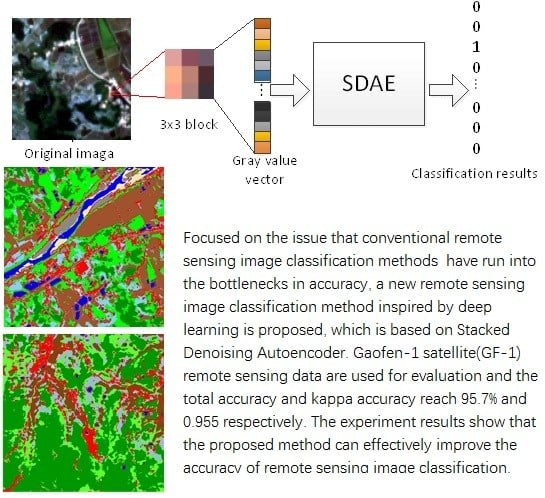
Focused on the issue that conventional remote sensing image classification methods have run into the bottlenecks in accuracy, a new remote sensing image classification method inspired by deep learning is proposed, which is based on Stacked Denoising Autoencoder. First, the deep network model is built through the stacked layers of Denoising Autoencoder. Then, with noised input, the unsupervised Greedy layer-wise training algorithm is used to train each layer in turn for more robust expressing, characteristics are obtained in supervised learning by Back Propagation (BP) neural network, and the whole network is optimized by error back propagation. Finally, Gaofen-1 satellite (GF-1) remote sensing data are used for evaluation, and the total accuracy and kappa accuracy reach 95.7% and 0.955, respectively, which are higher than that of the Support Vector Machine and Back Propagation neural network. The experiment results show that the proposed method can effectively improve the accuracy of remote sensing image classification.

Graphical Abstract

1. Introduction

Remote sensing image classification has always been a hot spot in remote sensing technology. It refers to the process of assigning each pixel in the remote sensing image to a semantic interpretation of the land cover or land use category. With the rapid increase in the amount of remote sensing image data and the gradual improvement in resolution, remote sensing image classification technology plays an increasingly important role in urban planning, environmental protection, resource management, mapping, and other fields. In general, remote sensing image classification is mainly divided into parametric and nonparametric methods [1]. Since parametric classifier requires knowing the distribution of data in advance, this is often difficult to achieve in remote sensing images. Therefore, the nonparametric classifier has been widely used, including artificial neural network, expert system, Support Vector Machine (SVM), decision tree, and so on [2,3,4,5,6]. All of the above methods, however, require analysis and extraction of a manually designed feature, and the overall classification accuracy is to be improved.
In recent years, with the difficulty in training problem of the deep neural network successfully solved by Hinton et al. [7,8], deep learning has widely concerned researchers, and has gradually been an upsurge in internet big data and artificial intelligence. The deep neural network is used to simulate the multi-layer structure of the human brain, abstract the original data layer by layer, and finally obtain the features suitable for classification. Today, deep learning has achieved great success in handwriting character recognition, speech recognition, and other fields, and it also provides a new idea for remote sensing image recognition technology. Presently, Hinton [9] used the DBN model to realize the road recognition of airborne remote sensing images. Wang et al. [10] used SAE to extract water from remote sensing images. Tang et al. [11] used a deep neural network for ship detection. Convolution neural networks have been widely used in remote sensing for scene classification [12], image segmentation [13] and target classification in SAR data [14], and recurrent neural network is utilized for learning land cover change [15]. Stacked Denoising Autoencoder (SDAE), an improved model of SAE, has made outstanding achievements in areas such as speech recognition [16] and other domains. Its excellent capacity for feature abstraction can be also utilized in remote sensing image classification so as to reach the higher accuracy just like it did in other domains. However, it has not been found that SDAE is used for relevant research of remote sensing classification.
In this paper, a remote sensing image classification method based on SDAE is proposed and verified by GF-1 remote sensing data. The experiment results show that the proposed method can achieve better classification effect compared with SVM and BP neural network.

2. Stacked Denoising Autoencoder Model

Stacked Denoising Autoencoder was proposed by Pascal Vincent el al. in 2010 [17], the core idea of which is to add the noise through each layer of the encoder input to train and learn more robust feature expression. From the structural point of view, SDAE is composed of a multi-layer of unsupervised denoising autoencoder network and a layer of supervised BP neural network. Figure 1 is the schematic of SDAE.
The learning process of SDAE has two steps: unsupervised learning and supervised learning. First, unlabeled samples are used for denoising autoencoder’s greedy layer-wise training, in which raw data is used to feed the first layer of DAE for unsupervised training, and then the parameter w ( 1 ) of the first hidden layer is obtained. In each subsequent step, the front k 1 trained layers as input are used to train the k th layer and obtain the parameter w ( k ) . The weight from training of each layer is taken as the weight of the final deep network’s initialization. Second, BP neural network with labeled data is carried out for supervised learning. While getting parameters of the associated feature and category of the last layer, the parameters of the entire network are fine-tuned by error back propagation so that the parameters converge to the position that is in or near the global optimum.

2.1. Denoising Autoencoder

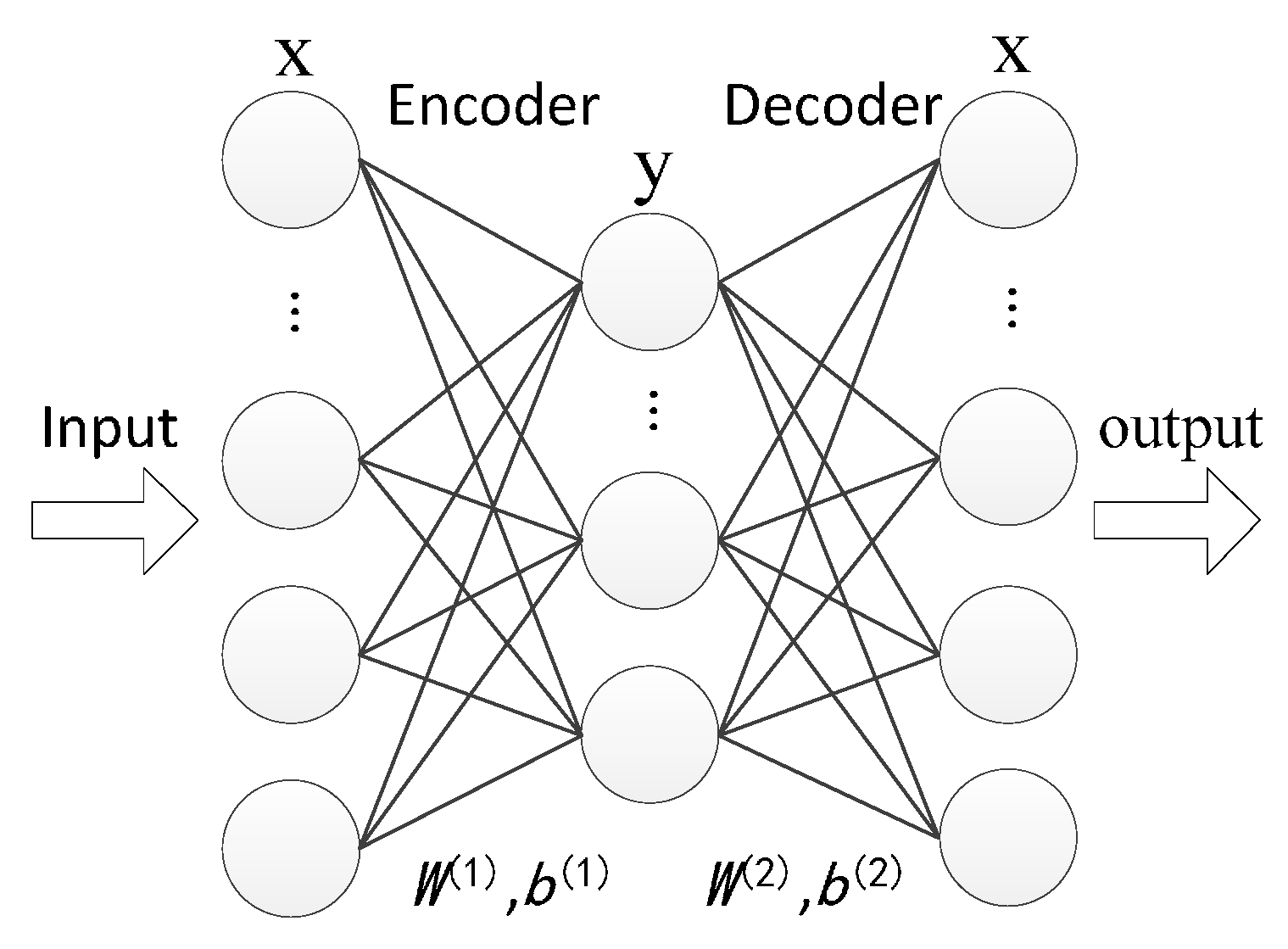
Autoencoder is a kind of unsupervised three-layer neural network [18], which consists of two parts of encoder and decoder, including an input layer, a hidden layer, and an output layer. The network structure is shown in Figure 2.
The role of the encoder is to map the input vector to the hidden layer and then get a new feature expression. The function is expressed as follows:
y = f ( x ) = s ( W ( 1 ) x + b ( 1 ) )
where x R d × 1 is input vector, d is the dimension of the input data, y R r × 1 , r is the number of hidden layer units, W ( 1 ) R r × d is the input weight for the hidden layer, and b ( 1 ) R r × 1 is the input bias for the hidden layer. s is the activation function, which is usually non-linear. The commonly used activation functions are sigmoid function s ( x ) = 1 1 + e x and tanh function s ( x ) = e x e x e x + e x .
The role of the decoder is to map the expression y of the hidden layer back to the original input. The function is expressed as follows:
x = g ( y ) = s ( W ( 2 ) y + b ( 2 ) )
where W ( 2 ) R d × r , b ( 2 ) R d × 1 . Thus, the reconstruction error for each data is
L = x g ( f ( x ) ) 2
Define the cost function as
J ( W , b ) = [ 1 N i = 1 N ( 1 2 x ( i ) g ( f ( x ( i ) ) ) 2 ) ] + λ 2 l = 1 2 i = 1 S l j = 1 S l + 1 ( W j i ( l ) ) 2
where x ( i ) is the i th sample, W j i ( l ) is connection weight between the i th unit of the l th layer and the j th unit of the ( l + 1 ) th layer, N is the number of samples, and S l is the number of units in the l th layer.
The optimal solution W and b of the model can be obtained by the error back propagation and the batch gradient descent algorithm.
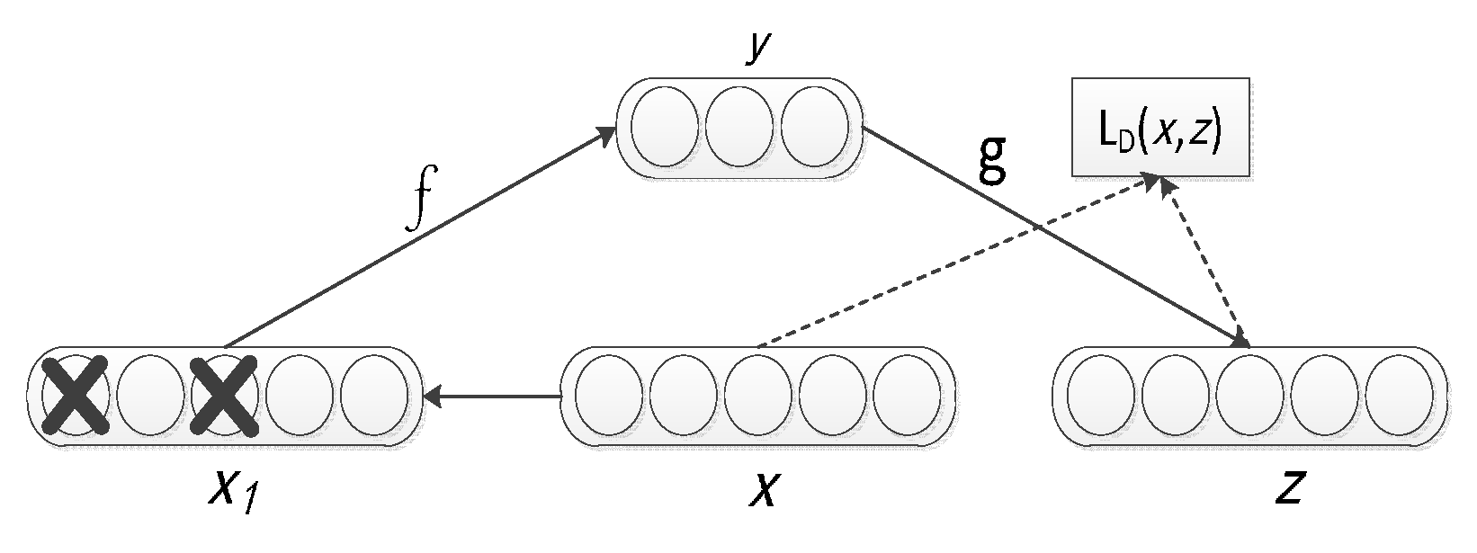
Denoising Autoencoder (DAE) is based on the autoencoder. Noise (Gaussian noise generally, or setting the data to zero randomly) will be added to the training data, and the autoencoder is forced to learn to remove noise so that uncontaminated input data can be obtained. In the case of corrupted input, the autoencoder can find more stable and useful features, which constitute a more advanced description of the input data, and enhance the robustness of the entire model. The principle of denoising training is shown in Figure 3:
In Figure 3, x is the initial input data, x 1 is the corrupted input data, y is the new feature obtained by encoding x 1 , and z is the output obtained by decoding y . The reconstruction error is
L D = x g ( f ( x 1 ) ) 2
The cost function is
J D ( W , b ) = [ 1 m i = 1 N ( 1 2 x ( i ) g ( f ( x 1 ( i ) ) ) 2 ) ] + λ 2 l = 1 2 i = 1 S l j = 1 S l + 1 ( W j i ( l ) ) 2
In general, we only need to randomly set the units in x to zero according to the noise figure k   ( k [ 0 ,   1 ] ) , and then x 1 will be obtained. The method of solving the parameters is the same as that of the autoencoder.

2.2. BP Neural Network

The BP neural network proposed by scientists Rumelhart el al. in 1986 [19] is a multi-layer feedforward network trained by an error back propagation algorithm. In this paper, we use the BP neural network for supervised classification of the features learned by DAE with labeled data. The feature vector can be associated with the corresponding label. At the same time, through the error back propagation, the parameters of the DAE will be fine-tuned, so that the entire network can converge further. The training of the BP neural network is mainly divided into two processes: forward propagation and error back propagation. First, the input feature vector is calculated in the forward direction, and the predicted category is obtained at the output layer. Then, the predicted category is compared with the actually corresponding category to get the classification error. After this, the parameters of the BP neural network are trained by error back propagation algorithm, and the parameters of DAE in each layer will be fine-tuned.
In the process of error back propagation, the residual δ (which denotes the contribution to the error) of each layer is calculated first. For each output unit i of the output layer, the formula of δ is
δ i = a i ( 1 a i ) ( a i y i )
For the other hidden layers, the formula of δ is
δ i l = a i l ( 1 a i l ) j = 1 S l + 1 W j i l δ i l + 1
where l is the l th layer of network, S l + 1 is number of the neurons of the ( l + 1 ) th layer, a i l is the output value of the i th unit of the l th layer.
After calculating the residuals of each layer, tune the parameters of the SDAE network layers according to Equations (9) and (10), α is the tuning coefficient.
W j i l = W j i l α a i l δ i l + 1
b i l = b i l α δ i l + 1

3. Remote Sensing Image Classification Method Based on SDAE

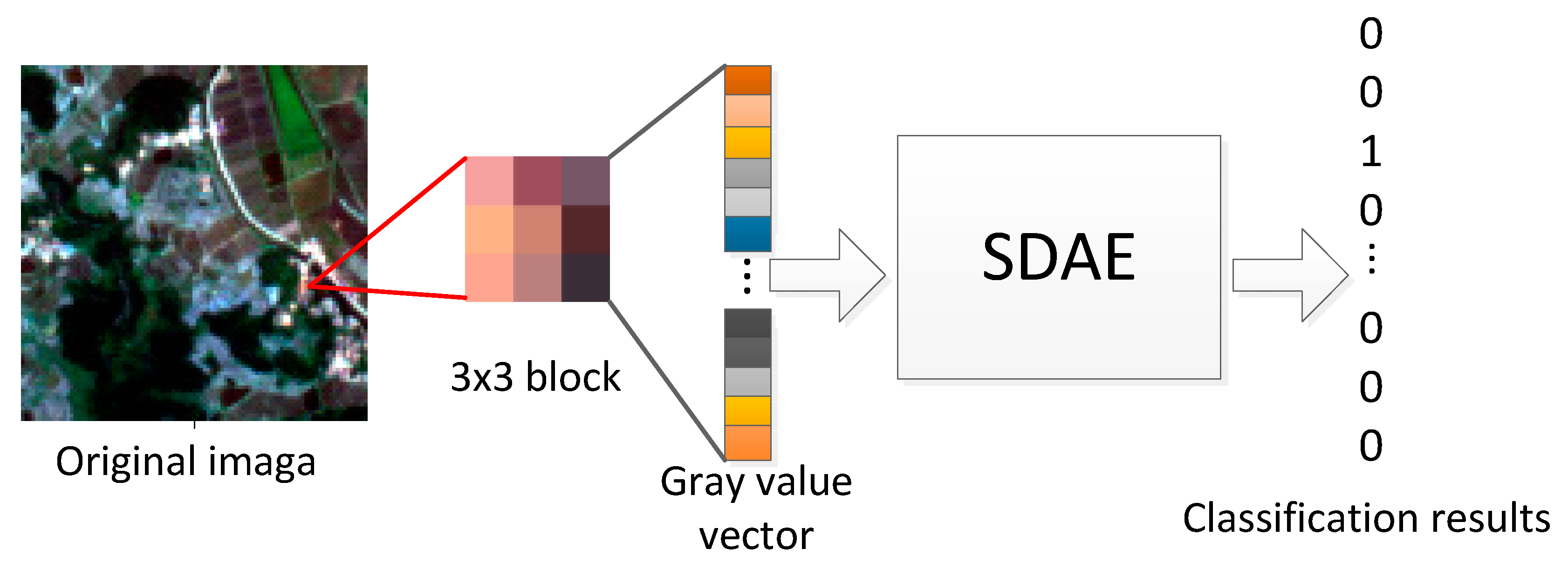
The purpose of remote sensing image classification in this paper is determining every pixel of image into a land cover category, and the result is supposed to be consistent with the ground truth. Because of the spatial correlation between each pixel and its neighboring pixels, such as texture, shape, etc., we use a S × S square image block centered on the point to be classified as the input of SDAE, which can avoid the interference of noise (Gaussian noise, speckle noise, and so on) with classification. The image block contains a variety of information such as spectrum, texture, shape, and so on. SADE can implicitly learn these features and use them for classification without the manual extraction of features. The larger the S is, the more information the image block contains, which is more conducive to classification. However, when the S is too large, there may be a variety of objects in an image block to affect the classification results. Based on the resolution of the experimental data, we choose the 4-band gray value of the 3 × 3 image block as the input for SDAE’s learning. So, the dimension of the input vector is 3 × 3 × 4 . The label of each image block is a vector whose dimension is the total number n of categories. Each node of the vector only takes two values: 0 and 1. If the image block belongs to the m th category, the m th number of the vector is set to 1, and the others are 0. Similarly, if the m th number of the output vector of SDAE is the largest, it denotes that the input image block is classified as the m th category. The process of our method is shown in Figure 4.

4. Results and Discussion

4.1. Experimental Data

In this paper, GF-1 remote sensing data is adopted, and the image resolution is 8 m (4-band in total). The study area is Qichun County, Hubei Province. The geographical coordinates are 115.6 degrees east longitude and 30.2 degrees north latitude. The main categories of this land cover are forest, grass, water, bare land (BL), architecture (ARC), sand ground (SD), crop, and river shoal (RS). BL mainly refer to soil or sparsely vegetated ground. The difference between SD and RS is that SD is above water and RS is under water. The ground truth is obtained manually using Google Earth. Experiment data is a 4548 × 4544 pixels image which is divided into two disjoint parts: one part is testing area that is formed by two 300 × 300 image patches with different terrain, and the other part is the rest of image that is used for training. The training and testing areas are separated to validate the robustness of the proposed approach. The experimental training samples are randomly selected from the training area with a total of 9410 blocks, of which the number of samples belonging to each object category is positively correlated with the actual number of such objects of this category. After the model trained, two 300 × 300 areas that are called testing area, above, are selected from the original image as the test image. The one area is flatland, the other is mountainous area, and 4800 points of each area are randomly and uniformly selected for the confusion matrix’s construction to evaluate the accuracy.

4.2. Evaluation Index for Classification Accuracy

In general, the confusion matrix is used to evaluate the classification accuracy of remote sensing images. The confusion matrix is shown below.
M = [ m 11 m 21 m 12 m 22 m 1 n m 2 n m n 1 m n 2 m n n ]
where m i j is the number of that the pixel of the actual object category i in the test area is assigned to the category j . n is the total number of categories, and m i i is the total number of that pixels belonging to the category i are correctly classified.
In this paper, we use the overall accuracy and kappa coefficient to evaluate the classification accuracy. The expression of the overall accuracy is
OA = i = 1 n m i i j = 1 n i = 1 n m i j
From Equation (12), it can be seen that the magnitude of the overall accuracy is only affected by the diagonal elements, and it is more likely to be affected by categories that contain more elements, so it is not sufficient to comprehensively evaluate the classification accuracy of all categories. Researchers have proposed the comprehensive index of classification accuracy’s evaluation, which is the kappa coefficient that utilizes all elements of the confusion matrix and reflects the consistency between classification result and ground truth. The expression of kappa coefficient is
K = N i = 1 n m i j i = 1 n m i + m + i N 2 i = 1 n m i + m + i
where N is the total number of pixels, n is the total number of categories, and m i + and m + i represent the sum of the elements of the ith row and the sum of the i t h column of the confusion matrix, respectively.

4.3. Results and Discussion

In our experiment, we study the following aspects:
  • The impact of the amount of hidden layers in the network and the neural units per layer on remote sensing image classification results;
  • The impact of the denoising process on classification ability of the model;
  • Comparison with SVM and the conventional artificial neural network.

4.3.1. The Impact of the Amount of Hidden Layer and the Neurons per Layer

The role of SDAE is to extract new features by multi-layer abstraction of original data. With the increase in the number of layers, SDAE can use the limited neural units to train to get more complex model, so as to learn more high-order features. These abstract features can describe the target more fundamentally. When the number of layers is too large, it is easy to overfit that the target is described with an overly complex model. Therefore, the selection of the network depth depends on the complexity of the actual condition. There is currently no guiding principle for the selection of the number of neurons in each hidden layer. When the number of neurons in hidden layer is small, the characteristic of the data cannot be adequately learned, while the large number of neurons will also result in overfitting and a large increase in the learning time of the network. In this paper, we choose 1 to 4 hidden layers in the network in this experiment. The number of neurons per layer is selected from 60 to 600, noise figure k is 0.5. The experimental results are shown in Figure 5.
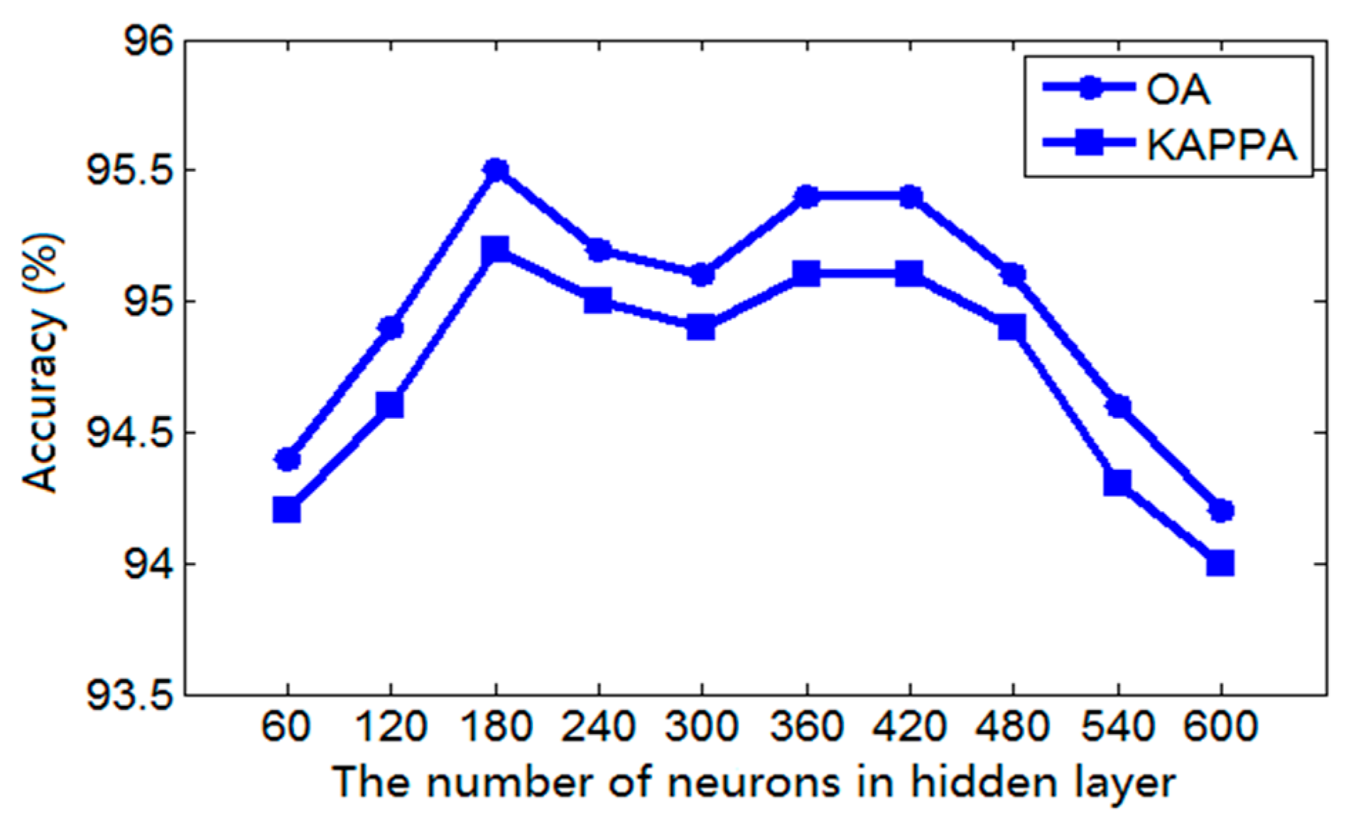
As shown in Figure 5, when the number of hidden layers is 2, the classification result is better. At this point, we use the SDAE network with 2 hidden layers and change the number of neurons per layer to do the experiment again. The experimental results are shown in Figure 6, where it can be seen that when the number of units in each hidden layer is 180, the overall accuracy and Kappa accuracy is largest. In addition, with the increase of the number of hidden layer units, the training time will increase rapidly.

4.3.2. The Impact of Denoising Pre-Training on Classification Ability of the Model

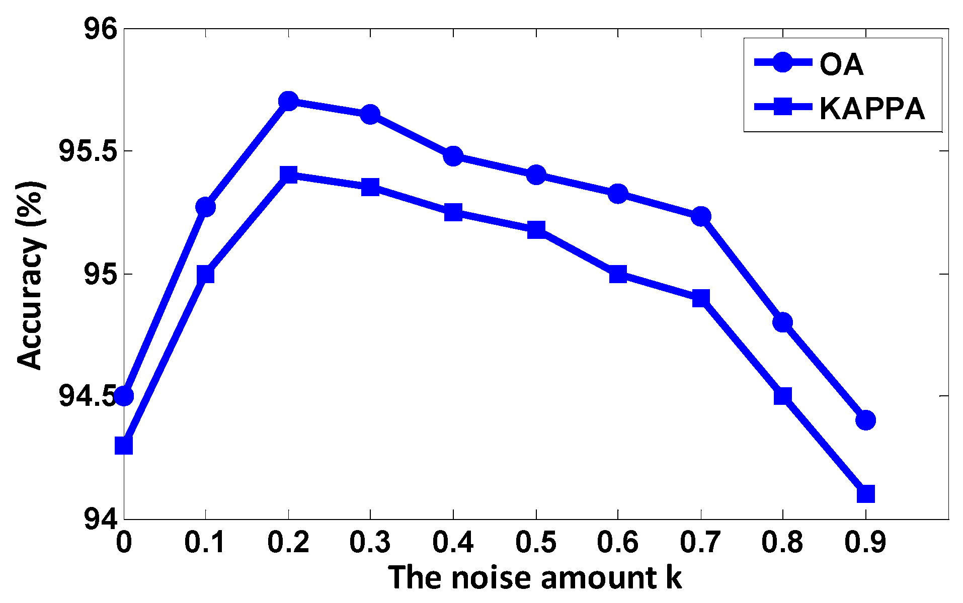
In the pre-training process of SDAE, in order to learn more useful features from the original data and enhance the robustness of the model, noise was manually added to the DAE input of each layer. Specifically, according to the proportion k, the input unit of DAE is randomly set to 0 in each training process, while AE of each layer in SAE directly uses training data. In order to explore the effect of denoising pre-training and the impact of different levels of noise added to the training data on the classification ability of the model, we choose a different k ranging from 0 to 1 for the experiment and compare the experimental results with SAE. The selected SAE model has the same network structure as that of SDAE model, the number of hidden layers is 2, and each layer has 180 units. The experimental results are shown in Figure 7.
In Figure 7, when k is 0, the ordinate value is the classification accuracy of SAE. We can conclude that a reasonable level of denoising pre-training significantly improves the classification accuracy of the model. When the noise figure k is 0.2, the classification accuracy of SDAE is the highest, and when it is greater than 0.9, the accuracy is lower than that of SAE, which indicates that noisy training data will reduce the learning ability of the model and result in the decrease of classification accuracy.

4.3.3. Comparison with Conventional Remote Sensing Images Classification Method

According to the experimental result of Section 4.3.1 and Section 4.3.2, it can be determined that when the number of SDAE’s hidden layers is 2, the number of units of each layer is 180, and the denoising coefficient is 0.2, classification performance is optimal. In order to verify the superiority of the proposed method, the classification results are compared with that of conventional methods: the SVM and BP neural network. The SVM model is established by the open source libsvm toolbox, the radial basis function is selected as kernel function, the optimal gamma parameters are obtained by grid search and cross validation, and the classification results at this time are taken as the final results. The search range in experiment is 0.1 to 5, and the optimal gamma is 0.6. The BP neural network uses the same network structure as SDAE, with a topology of 36-180-180-8. The experimental results are shown in Table 1. The results of remote sensing image classification based on SDAE are obviously better than the other two methods, whether it is evaluated according to OA accuracy or KAPPA accuracy.
Compared to the BP neural network, the initial connection weights of the SDAE network are obtained by layer-wise pre-training rather than random initialization. By pre-training, the initial connection weights are in the vicinity of the optimal value, and then, through fine-tuning, the weights can converge to the ideal value. The BP neural network’s random initialization easily results in the fact that parameters are difficult to converge to ideal value or even fall into the local minimum value in the training process, which leads to training failure. This is more easily reflected in the training of the deep network, so the classification results of SDAE are better than those of the BP neural network. SDAE has stronger classification ability than SVM because its deep nonlinear network abstracts the original data layer by layer and gets the features that can describe the nature of the object better, which makes them easily classified. The robustness of the extracted features is further increased by denoising pre-training of DAE per layer, and the spatial features of the remote sensing data are more fully excavated. In terms of time, SDAE takes more than SVM because almost all of deep network models require a large number of iterations to make the parameters converge to the optimal value.
Table 2 and Table 3 are the confusion matrixes from classification results using SDAE for flatland area and mountainous area respectively. It can be seen that in both results Water, Forest, BL, and Crop have the classification accuracy over 96%, and that of ARC is only 88% and 90.3%. A considerable part of ARC is wrong classified as SD. This is because different buildings have many ways of performance in the image, and the features of some kinds of buildings are similar to that of sand ground.
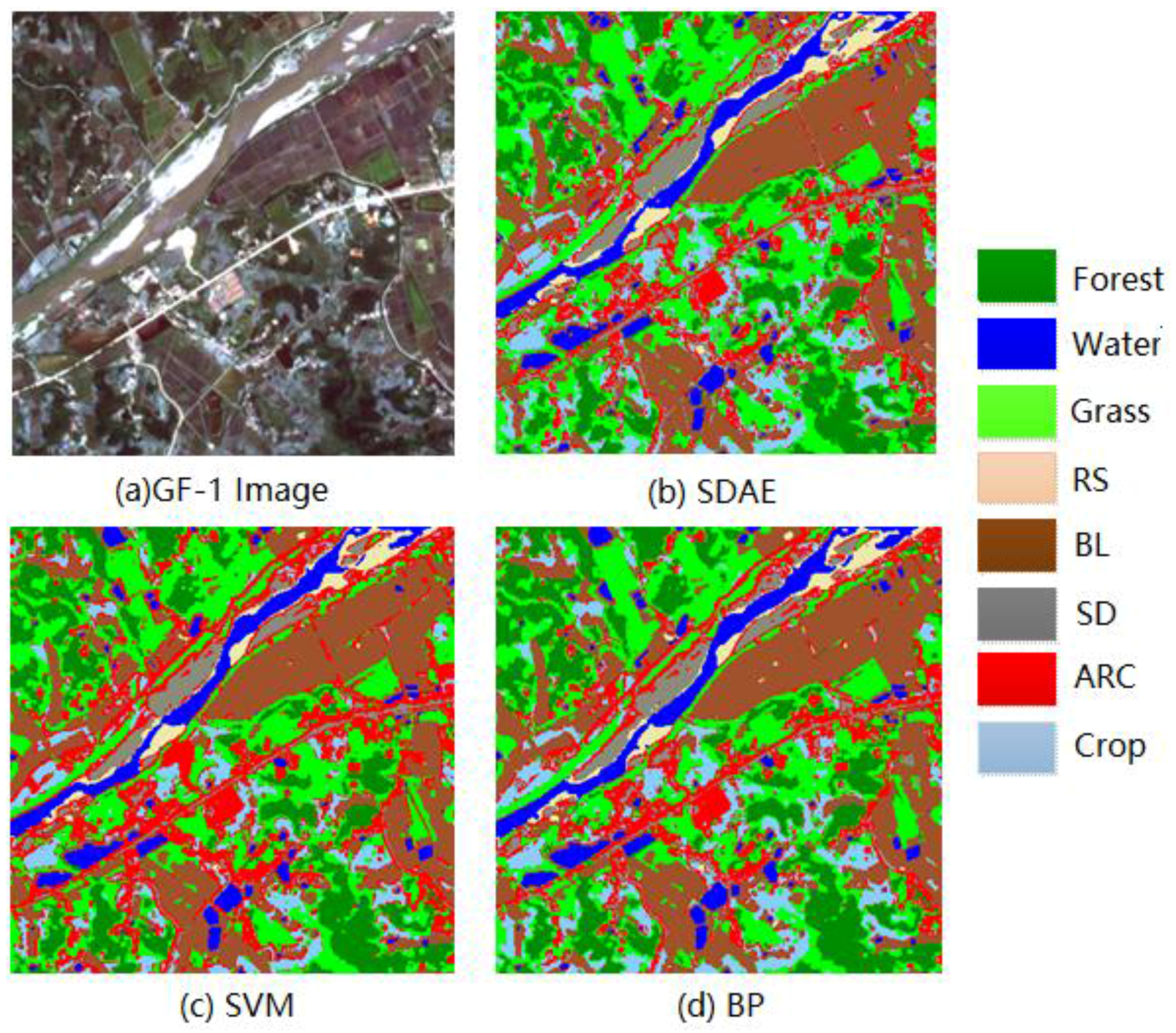
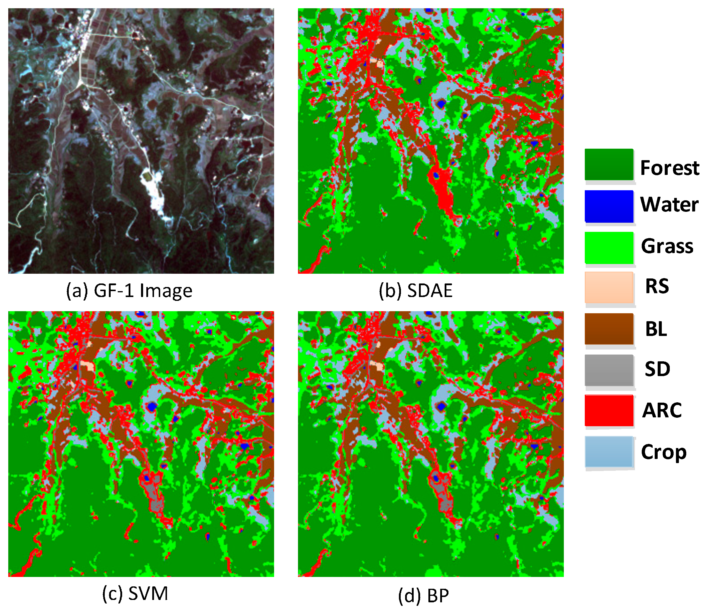
Figure 8 shows the classification results of the flatland area by several methods. We can see that compared with the SVM and BP neural network, DAE significantly reduces the number of pixels that belong to BL, SD, or Crop, but wrongly classified them as the ARC category. In addition, the classification accuracy of SD has been significantly improved, which indicates that the method based on SDAE can better preserve the details of the objects than other conventional methods. Figure 9 is the classification results of the mountainous area. It can be observed obviously that many ARC pixels are wrongly classified as SD in the results of SVM and BP, but they are correctly determined by SDAE.

5. Conclusions

In this paper, a remote sensing image classification method based on SDAE is proposed. First, greedy layer-wise training is used for training every layer except the last of SDAE. This step is unsupervised, and it is fed with image data without label. Noise is put into data so the model could be more robust. Then, a back propagation algorithm is used for training the total network, the last layer is trained, and others are fine-tuned. Finally, the SDAE model is used for determining the category of every block in the test area, and accuracy assessment is done. With GF-1 remote sensing data in experiment, the SDAE model achieves better classification results than the classical model SVM and BP neural network but also results in a larger time cost. Since the time cost will certainly constrain the application of a large-scale and deep SDAE model, we will compare SDAE with other deep learning methods in the future and try to use the parallelization framework to improve the accuracy and speed of remote sensing image classification.

Author Contributions

Peng Liang and Wenzhong Shi conceived and designed the experiments; Peng Liang performed the experiments; Peng Liang and Wenzhong Shi analyzed the data; Xiaokang Zhang contributed materials and analysis tools; Peng Liang wrote the paper.

Conflicts of Interest

The authors declare no conflict of interest.

References

  1. Jia, K.; Li, Q.Z.; Tian, Y.C.; Wu, B.F. A Review of Classification Methods of Remote Sensing Imagery. Spectrosc. Spectr. Anal. 2011, 31, 2618–2623. [Google Scholar]
  2. Srivastava, P.K.; Han, D.; Rico-Ramirez, M.A.; Bray, M.; Islam, T. Selection of classification techniques for land use/land cover change investigation. Adv. Space Res. 2012, 50, 1250–1265. [Google Scholar] [CrossRef]
  3. Niu, X.; Ban, Y.F. Multi-temporal RADARSAT-2 polarimetric SAR data for urban land cover classification using an object based support vector machine and a rule-based approach. Int. J. Remote Sens. 2013, 34, 1–26. [Google Scholar] [CrossRef]
  4. Bazi, Y.; Melgani, F. Toward an optimal SVM classification system for hyperspectral remotesensing images. IEEE Trans. Geosci. Remote Sens. 2006, 44, 3374–3385. [Google Scholar] [CrossRef]
  5. Mishra, P.; Singh, D.; Yamaguchi, Y. Land cover classification of PALSAR images by knowledge based decision tree classifier and supervised classifiers based on SAR observables. Prog. Electromagn. Res. B 2011, 30, 47–70. [Google Scholar] [CrossRef]
  6. Gan, S.; Yuan, X.P.; He, D.M. An application of vegetation classification in Northwest Yunnan with remote sensing expert classifier. J. Yunnan Univ. (Nat. Sci. Ed.) 2003, 25, 553–557. [Google Scholar]
  7. Hinton, G.E.; Osindero, S. A fast learning algorithm for deep belief nets. Neural Comput. 2006, 18, 1527–1554. [Google Scholar] [CrossRef] [PubMed]
  8. Bengio, Y. Learning Deep Architectures for AI; Foundations and Trends® in Machine Learning; Now Publishers Inc.: Hanover, MA, USA, 2009; Volume 2, pp. 1–127. [Google Scholar]
  9. Mnih, V.; Hinton, G.E. Learning to detect roads in high resolution aerial images. In Proceedings of the 2010 European Conference Computer Vision, Heraklion, Crete, Greece, 5–11 September 2010; pp. 210–223. [Google Scholar]
  10. Wang, Z.Y.; Yu, L.; Tian, S.W.; Wang, Z.; Long, Y.U.; Tian, S.; Qian, Y.; Ding, J.; Yang, L. Water body extraction method based on stacked autoencoder. J. Comput. Appl. 2015, 35, 2706–2709. [Google Scholar]
  11. Tang, J.; Deng, C.; Huang, G.B.; Zhao, B. Compressed-domain ship detection on spaceborne optical image using deep neural network and extreme learning machine. IEEE Trans. Geosci. Remote Sens. 2014, 53, 1174–1185. [Google Scholar] [CrossRef]
  12. Hu, F.; Xia, G.S.; Hu, J.W. Transferring deep convolutional neural networks for the scene classification of high-resolution remote sensing imagery. Remote Sens. 2015, 7, 14680–14707. [Google Scholar] [CrossRef]
  13. Längkvist, M.; Kiselev, A.; Alirezaie, M.; Loutfi, A. Classification and segmentation of satellite orthoimagery using convolutional neural networks. Remote Sens. 2016, 8, 329. [Google Scholar] [CrossRef]
  14. Chen, S.; Wang, H.; Xu, F.; Jin, Y.Q. Target classification using the deep convolutional networks for SAR images. IEEE Trans. Geosci. Remote Sens. 2016, 54, 4806–4817. [Google Scholar] [CrossRef]
  15. Lyu, H.; Lu, H.; Mou, L. Learning a transferable change rule from a Recurrent Neural Network for Land Cover Change Detection. Remote Sens. 2016, 8, 506. [Google Scholar] [CrossRef]
  16. Noda, K.; Yamaguchi, Y.; Nakadai, K.; Okuno, H.G.; Ogata, T. Audio-visual speech recognition using deep learning. Appl. Intell. 2015, 42, 722–737. [Google Scholar] [CrossRef]
  17. Vincent, P.; Larochelle, H.; Lajoie, I.; Bengio, Y.; Manzagol, P.A. Stacked denoising autoencoders: Learning useful representations in a deep network with a local denoising criterion. J. Mach. Learn. Res. 2010, 11, 3371–3408. [Google Scholar]
  18. Baldi, P. Autoencoders, unsupervised learning, and deep architecture. In Proceedings of the ICML Workshop on Unsupervised and Transfer, Bellevue, WA, USA, 2 July 2011; Volume 27, pp. 37–50. [Google Scholar]
  19. Rumelhart, D.E.; Hinton, G.E.; Williams, R.J. Learning representations by back-propagation errors. Nature 1986, 323, 533–536. [Google Scholar] [CrossRef]
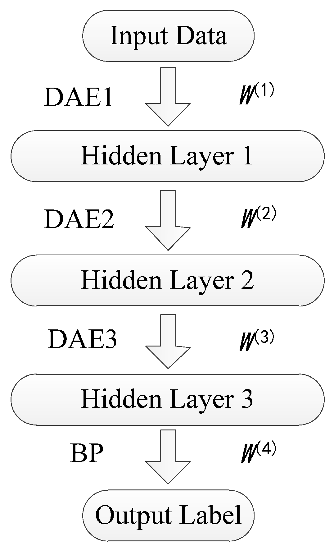
Figure 1. Stacked Denoising Autoencoder (SDAE).
Remotesensing 10 00016 g001
Figure 2. Autoencoder.
Remotesensing 10 00016 g002
Figure 3. The principle of denoising training.
Remotesensing 10 00016 g003
Figure 4. The process of Remote sensing image classification method based on SDAE.
Remotesensing 10 00016 g004
Figure 5. The impact of the number of SDAE hidden layers on classification accuracy.
Remotesensing 10 00016 g005
Figure 6. The impact of the number of neurons in hidden layers on classification accuracy.
Remotesensing 10 00016 g006
Figure 7. The impact of noise coefficient on classification accuracy.
Remotesensing 10 00016 g007
Figure 8. Classification results of flatland area by several methods.
Remotesensing 10 00016 g008
Figure 9. Classification results of mountainous area by several methods.
Remotesensing 10 00016 g009
Table 1. Comparison of classification results among different methods.
AreaClassSDAESVMBP
Flatland areaOA/%95.794.192.4
KAPPA0.9550.9360.921
mountainous areaOA/%96.294.293.7
KAPPA0.9580.9370.936
Computation Time/s51.247.158.4
Table 2. Confusion matrix of classification results using SDAE for a flatland area.
ClassClassification ResultTotalAccuracy/%
ForestWaterGrassRSBLSDARCCrop
Forest72001604 00074097.3
Water045202002055699.1
Grass426860428471096.4
RS21804500010448493.0
BL042074228075897.9
SD2000041224244093.6
ARC00084444821255088.6
Crop0202001264666297.6
Total7284787044627544605466684800100
Table 3. Confusion matrix of classification results using SDAE for a mountainous area.
ClassClassification ResultTotalAccuracy/%
ForestWaterGrassRSBLSDARCCrop
Forest228784507 041235297.2
Water0310010003296.9
Grass1408260408485696.6
RS0000000000
BL315258809361196.2
SD 000000000
ARC01311023408645290.3
Crop109060447749796.0
Total2305418883616234334914800100