Mapping Latent Heat Flux in the Western Forest Covered Regions of Algeria Using Remote Sensing Data and a Spatialized Model

Abstract
:1. Introduction
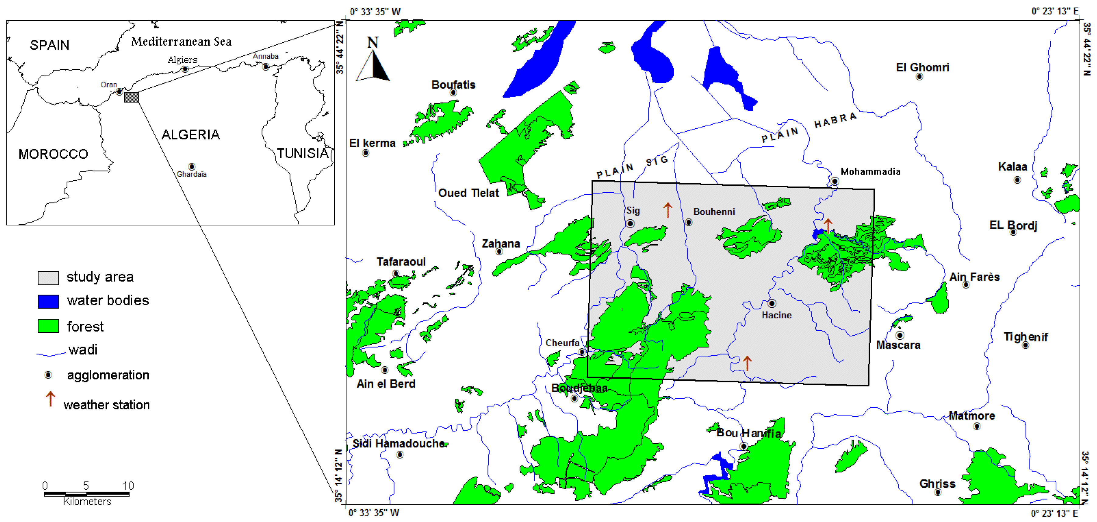
2. Site Description
3. Data Use and Input Parameters

| Parameter | Unit | TM day 150 |
|---|---|---|
| Solar declination | rad | 0.3797 |
| Sun-earth distance | AU | 1.0138 |
| Solar angle hour | rad | 0.3938 |
| Solar zenith angle | rad | 0.4187 |
4. Methodology for Estimating Latent Heat Flux

5. Results and Discussion
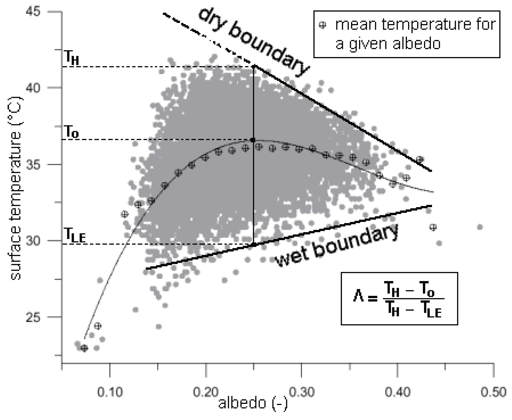
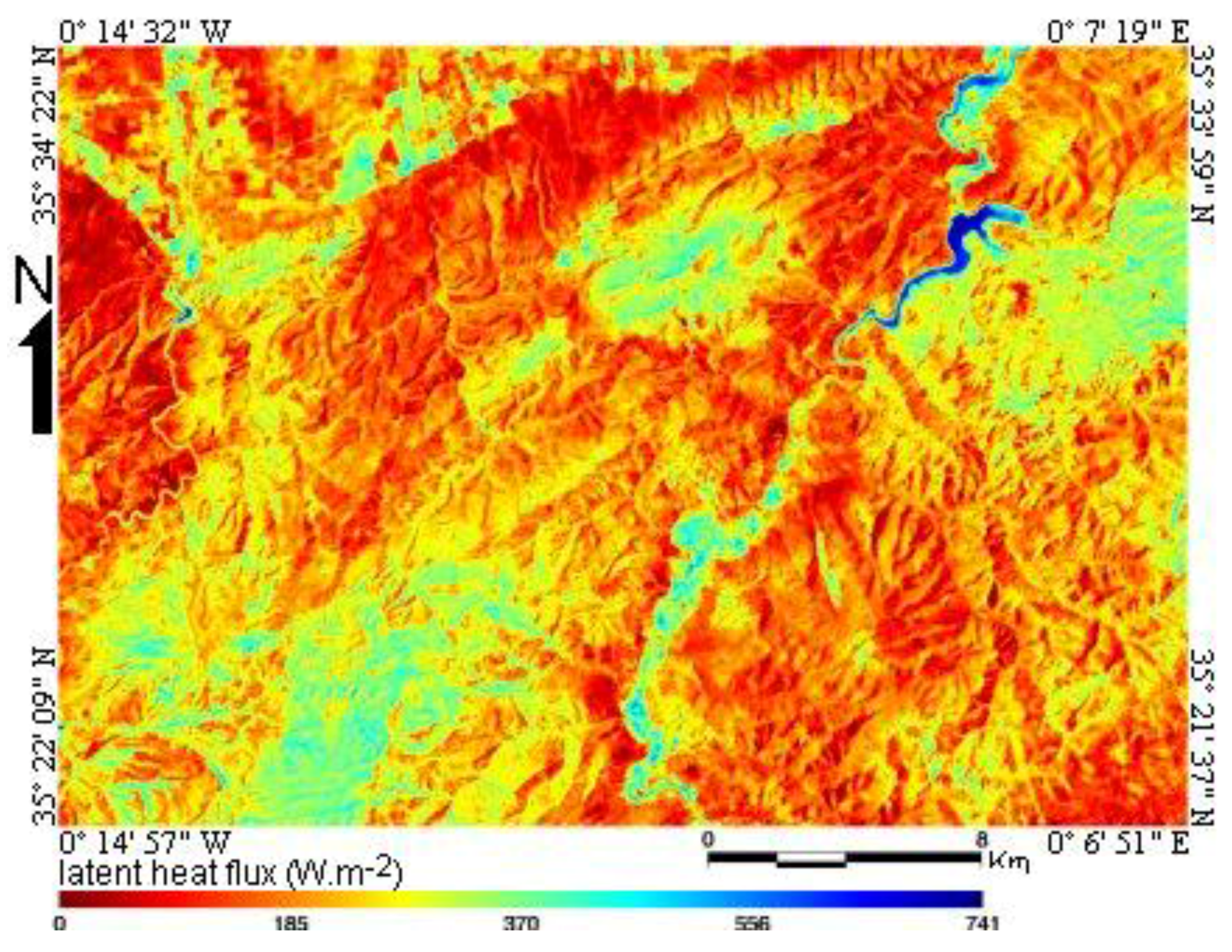
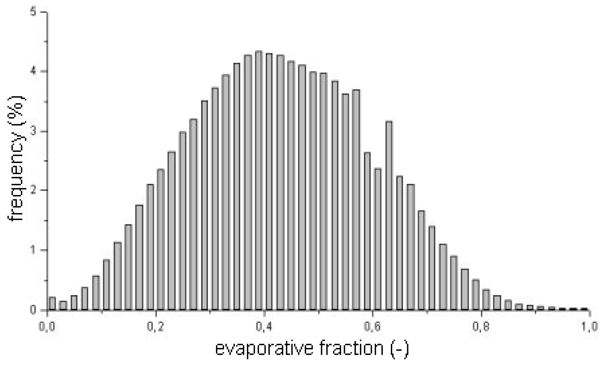
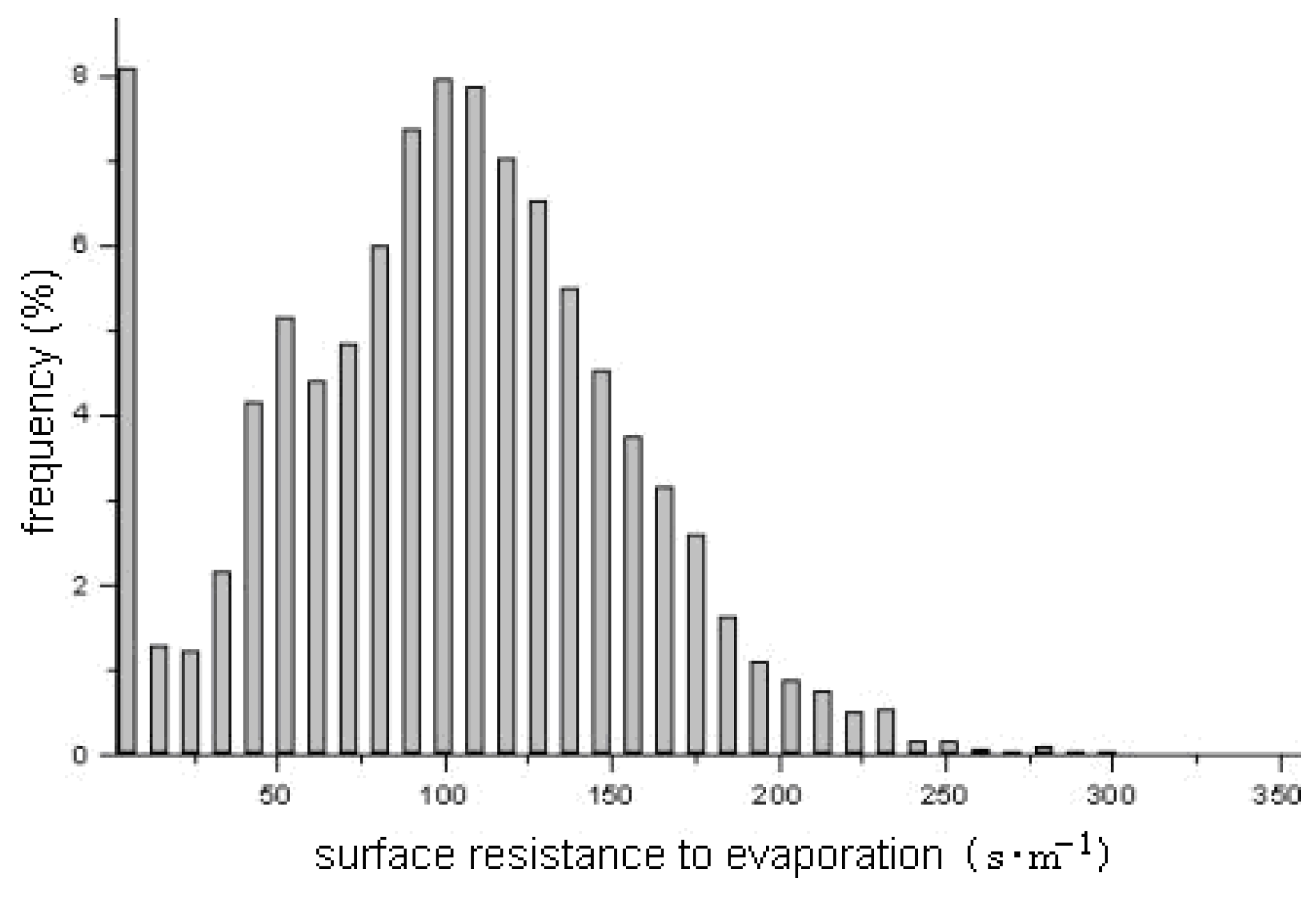
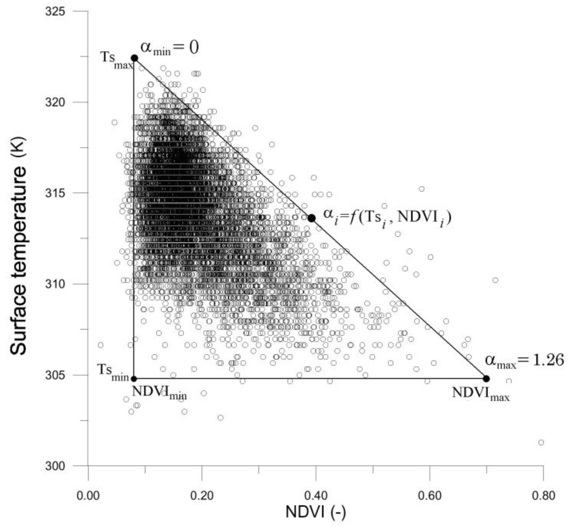
5.1. Results Obtained with S-SEBI Method
| Parameter | Unit | Dry pixels | Wet pixels |
|---|---|---|---|
| NDVI | – | 0.117 | −0.084 |
| Albedo | – | 0.310 | 0.120 |
| Surface temperature | K | 325.9 | 300.8 |
| Emissivity | – | 0.926 | 1.00 |
| Net radiation | W∙m−2 | 597.6 | 713.5 |
| Soil heat flux | W∙m−2 | 140.9 | 57.4 |
| Sensible heat flux | W∙m−2 | 466.6 | 0.0 |
| Latent heat flux | W∙m−2 | 0.0 | 656.1 |
| Evaporation Fraction | – | 0.0 | 1.0 |
| Near-surface air temperature difference | K | 295.9 | 275.2 |
| Aerodynamic resistance to heat transfer | s∙m−1 | 58.7 | 223.4 |
| Surface resistance to evaporation | s∙m−1 | 3990.6 | 0.0 |
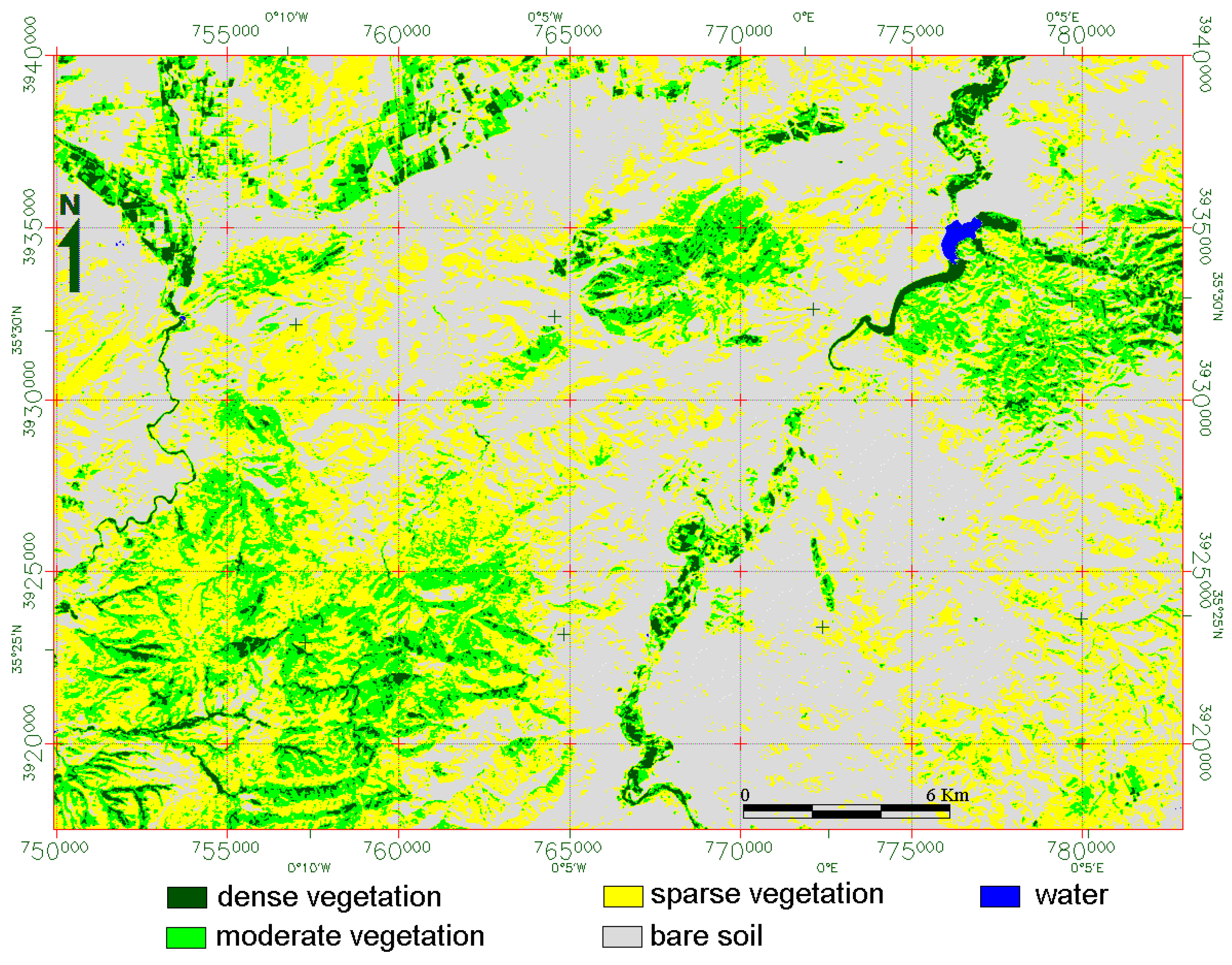
| Land use | Rn(W∙m−2) | G0(W∙m−2) | H(W∙m−2) | LE(W∙m−2) | Λ(–) |
|---|---|---|---|---|---|
| Water | 745.91 | 64.48 | 23.17 | 658.25 | 0.96 |
| Dense vegetation | 650.09 | 92.78 | 164.15 | 393.15 | 0.71 |
| Moderate vegetation | 636.57 | 105.41 | 222.82 | 308.33 | 0.58 |
| Sparse vegetation | 618.56 | 115.91 | 279.67 | 222.97 | 0.44 |
| Urban and bare soil | 583.18 | 119.61 | 296.86 | 166.69 | 0.36 |
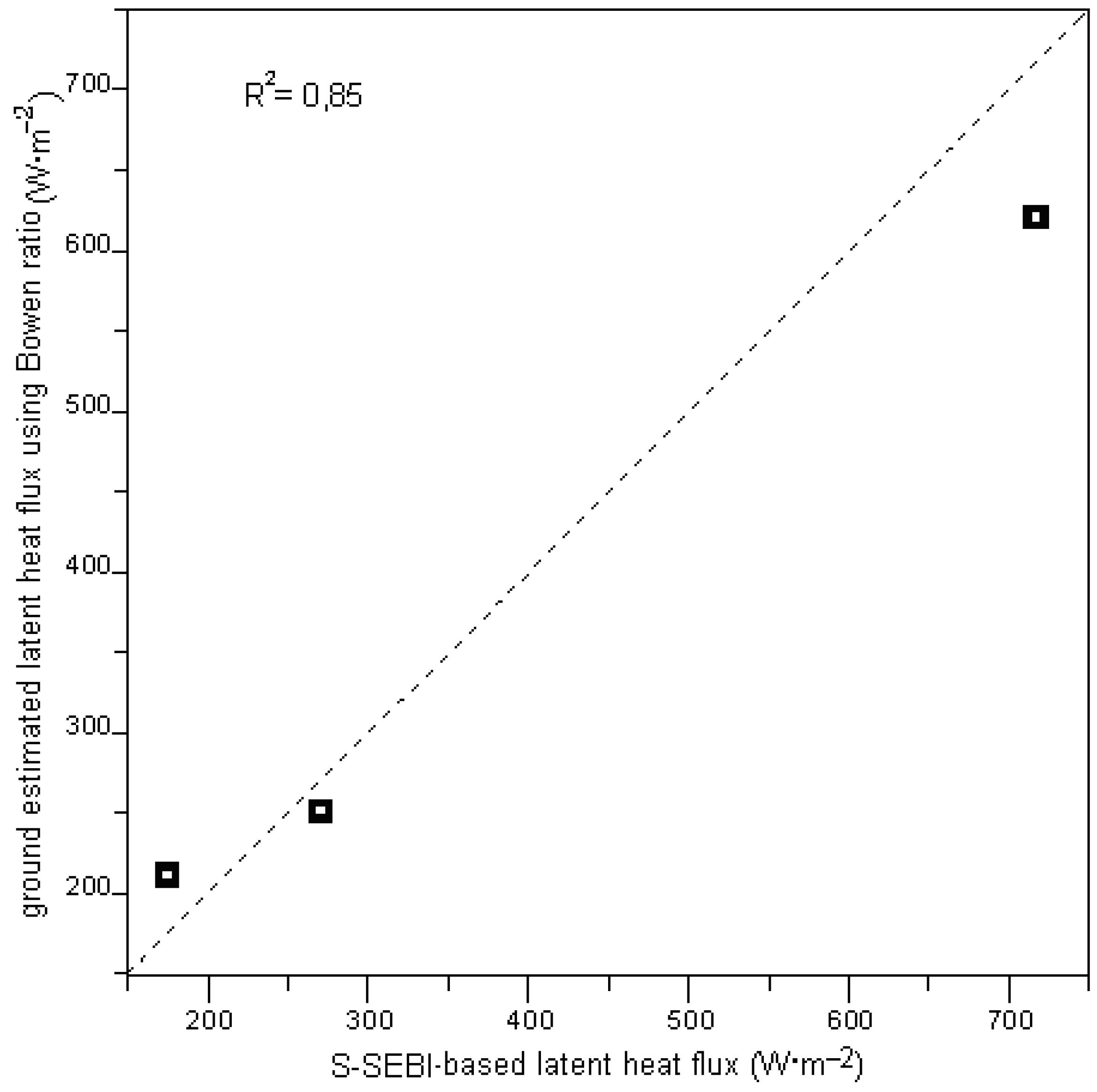
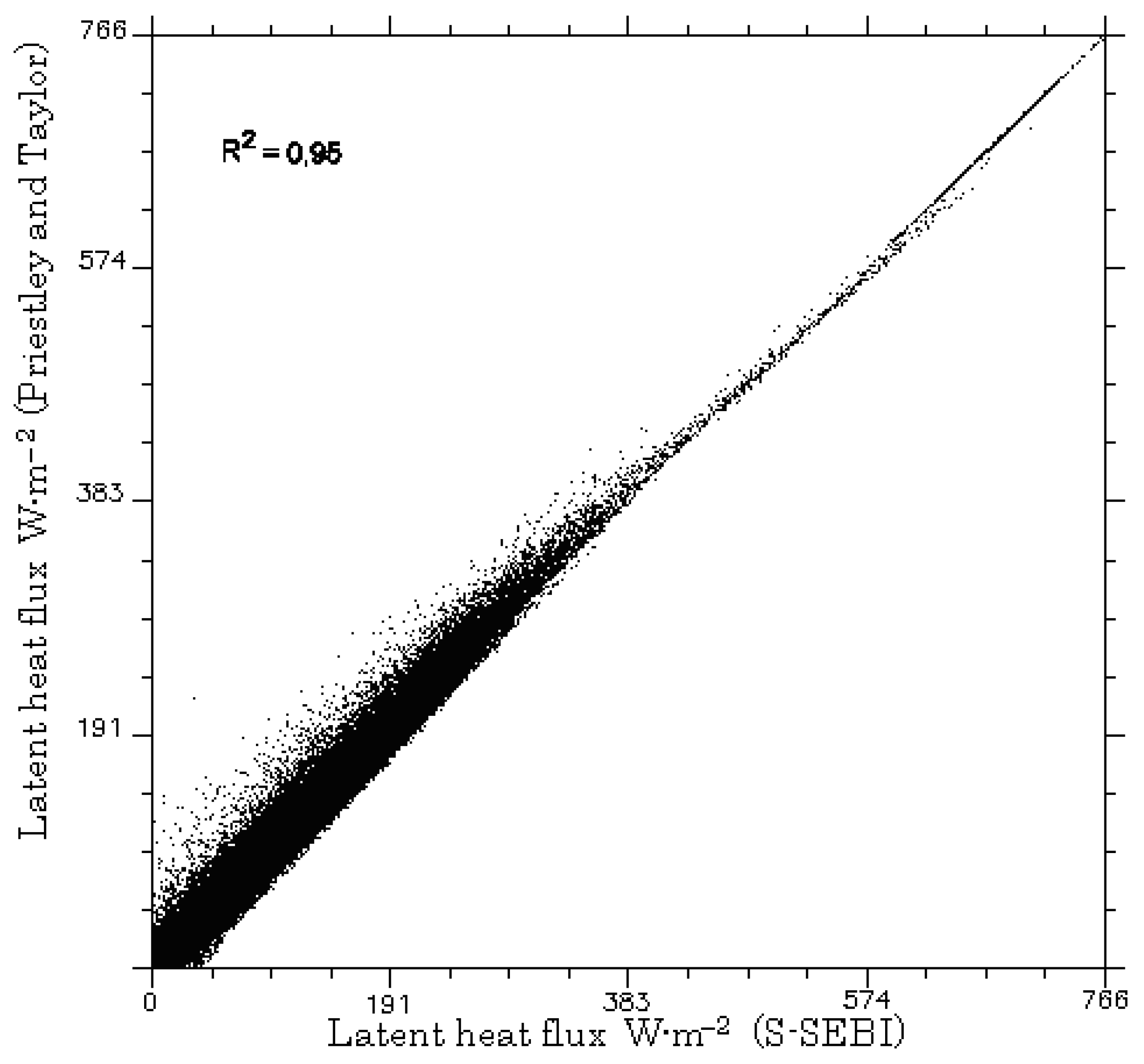
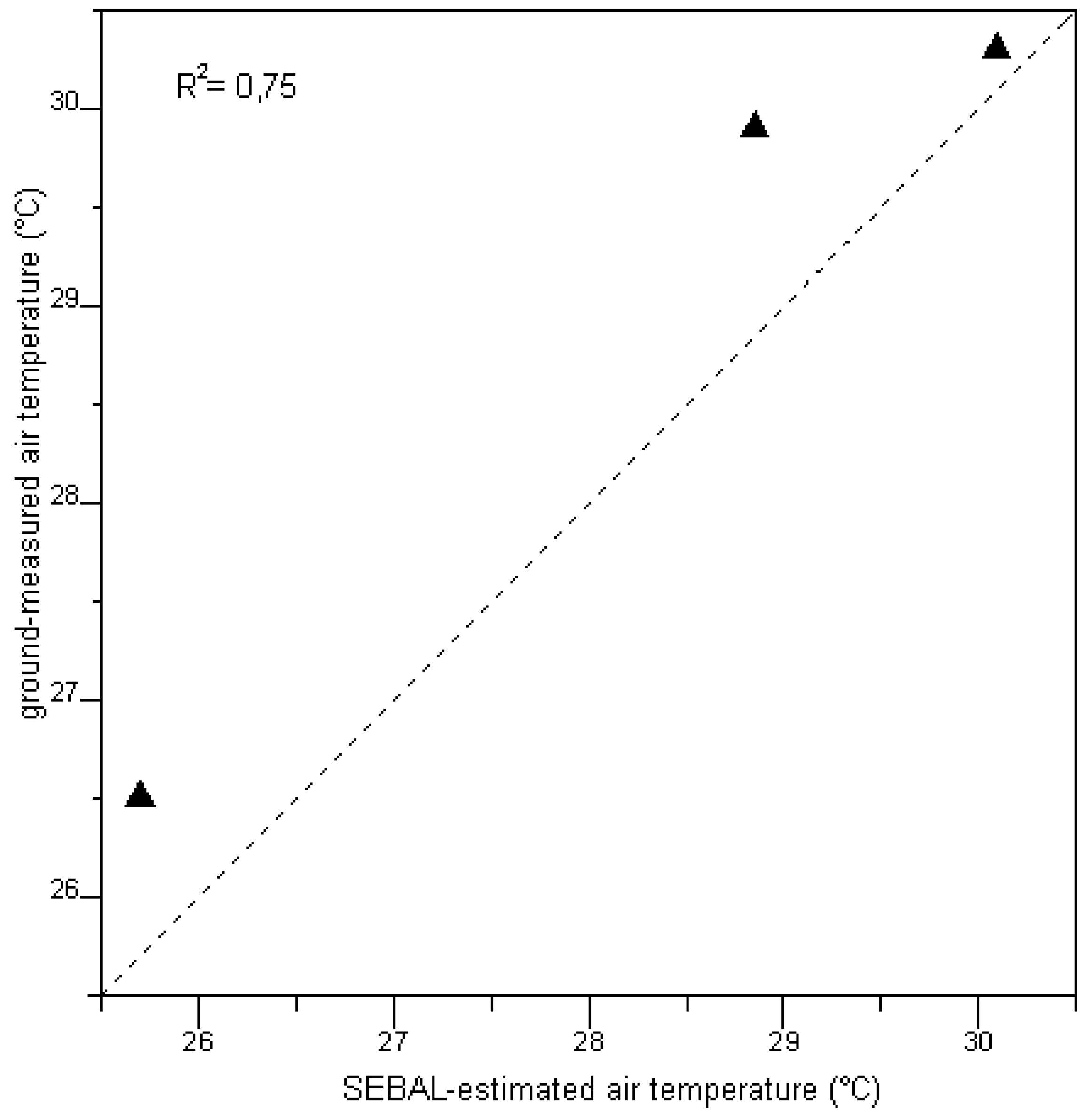
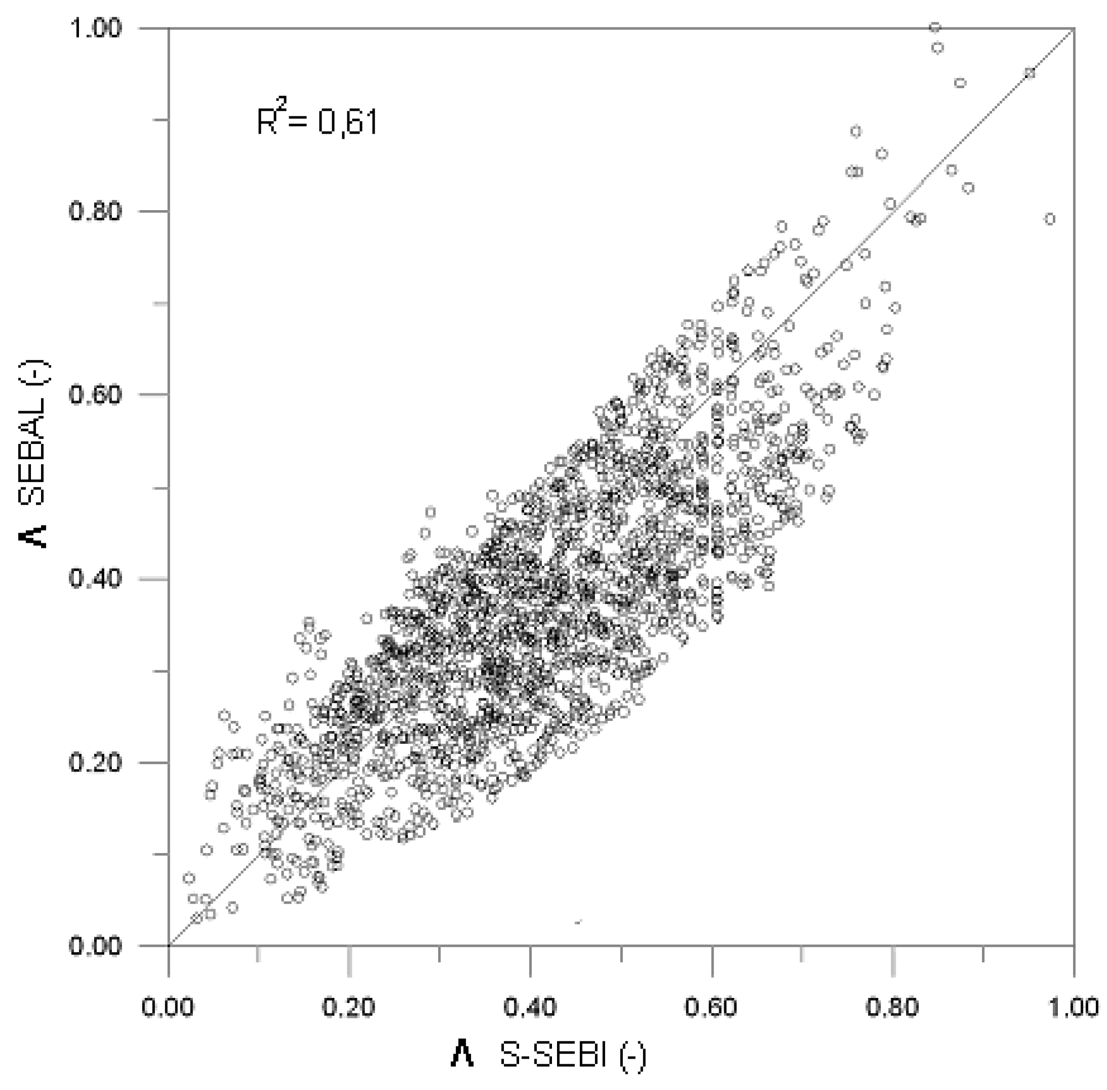
5.2. Evaluation Method


5.3. Sensitivity Analysis
6. Conclusions
Acknowledgements
References and Notes
- Peñuelas, J.; Filella, I.; Biel, C.; Serrano, L.; Save´, R. The reflectance at the 950–970 nm region as an indicator of plant water status. Int. J. Remote Sens. 1993, 14, 1887–1905. [Google Scholar] [CrossRef]
- Maki, M.; Ishiahra, M.; Tamura, M. Estimation of leaf water status to monitor the risk of forest fires by using remotely sensed data. Remote Sens. Environ. 2004, 90, 441–450. [Google Scholar] [CrossRef]
- Larcher, W. Physiological Plant Ecology. In Ecophysiology and Stress Physiology of Functional Groups, 3rd ed.; Springer: New York, NY, USA, 1995; p. 528. [Google Scholar]
- Jackson, R.D. Remote sensing of biotic and abiotic plant stress. Annu. Rev. Phytopathol. 1986, 24, 265–287. [Google Scholar] [CrossRef]
- Chuvieco, E.; Deshayes, M.; Stach, N.; Cocero, D.; Riaño, D. Short-Term Fire Risk: Foliage Moisture Content Estimation From Satellite Data. In Remote Sensing of Large Wildfires in the European Mediterranean Basin; Chuvieco, E., Ed.; Alcala´ University press: Madrid, Spain, 1999; p. 228. [Google Scholar]
- Desbois, N.; Pereira, J.M.; Beaudoin, A.; Chuvieco, E.; Vidal, A. Short Term Fire Risk Mapping Using Remote Sensing. In A Review of Remote Sensing Methods for the Study of Large Wildland Fires; Chuvieco, E., Ed.; Megafires: Alcala´, Spain, 1997; pp. 29–60. [Google Scholar]
- Clothier, B.E.; Clawson, K.L.; Pinter, P.J.; Moran, M.S.; Reginato, R.J.; Jackson, R.D. Estimation of soi1 heat flux from net radiation during the growth of alfalfa. Agr. Forest Meteorol. 1986, 37, 319–329. [Google Scholar] [CrossRef]
- Desbois, N.; Vidal, A. La télédétection dans la prévision des incendies de forêts. Ingénieries-EAT 1995, 1, 21–29. [Google Scholar]
- Jarvis, P.; James, G.; Landesburg, J. Coniferous Forest in Vegetation and the Atmosphere; Monteith, J.L., Ed.; Academic press: New York, NY, USA, 1976; Volume 2, pp. 171–236. [Google Scholar]
- Gao, B.C.; Goetz, A.F.H. Retrieval of equivalent water thickness and information related to biochemical components of vegetation canopies from AVIRIS data. Remote Sens. Environ. 1995, 52, 155–162. [Google Scholar] [CrossRef]
- Gao, B.C. NDWI-A normalized difference water index for remote sensing of vegetation liquid water from space. Remote Sens. Environ. 1996, 58, 257–266. [Google Scholar] [CrossRef]
- Peñuelas, J.; Piñol, J.; Ogaya, R.; Filella, I. Estimation of plant water concentration by the reflectance Water Index WI (R900/R970). Int. J. Remote Sens. 1997, 18, 2869–2875. [Google Scholar] [CrossRef]
- Zarco-Tejada, P.J.; Rueda, C.A.; Ustin, S.L. Water content estimation in vegetation with MODIS reflectance data and model inversion methods. Remote Sens.Environ. 2003, 85, 109–124. [Google Scholar] [CrossRef]
- Ustin, S.L.; Roberts, D.A.; Gamon, J.A.; Asner, G.P.; Green, R.O. Using imaging spectroscopy to study ecosystem processes and properties. BioScience 2004, 54, 523–534. [Google Scholar] [CrossRef]
- Peñuelas, J.; Filella, I.; Biel, C.; Serrano, L.; Savé, R. The reflectance at the 950–970 nm region as an indicator of plant water status. Int. J. Remote Sens. 1993, 14, 1887–1905. [Google Scholar] [CrossRef]
- Hamimed, A.; Mederbal, K.; Khaldi, A. Utilisation des données satellitaires TM de Landsat pour le suivi de l’état hydrique d’un couvet végétal dans les conditions semi-arides en Algérie. Télédétection 2001, 2, 29–38. [Google Scholar]
- Ustin, S.L.; Roberts, D.A.; Jacquemoud, S.J.; Pinzón, S.; Gardner, M.; Scheer, G.; Castaneda, C.M.; Palacios-Orueta, A. Estimating canopy water content of chaparral shrubs using optical methods. Remote Sens. Environ. 1998, 65, 280–291. [Google Scholar] [CrossRef]
- Chuvieco, E.; Cocero, D.; Riaño, D.; Martin, P.; Martınez-Vega, J.; Riva, J.; Perez, F. Combining NDVI and surface temperature for the estimation of live fuel moisture content in forest fire danger rating. Remote Sens. Environ. 2004, 92, 322–331. [Google Scholar] [CrossRef]
- Riaño, D.; Vaughan, P.; Zarco-Tejada, E.; Ustin, P.J. Estimation of fuel moisture content by inversion of radiative transfer models to simulate equivalent water thickness and dry matter content. Analysis at leaf and canopy level. IEEE Trans. Geosci. Remote Sens. 2005, 43, 819–826. [Google Scholar] [CrossRef]
- Petropoulos, G.; Carlson, T.N.; Wooster, M.J.; Islam, S. A review of Ts/VI remote sensing based methods for the retrieval of land surface energy fluxes and soil surface moisture. Prog. Phys. Geo. 2009, 33, 224–250. [Google Scholar] [CrossRef]
- Carlson, T.N.; Gillies, R.R.; Perry, E.M. A method to make use of thermal infrared temperature and NDVI measurements to infer surface soil water content and fractional vegetation cover. Remote Sens. Rev. 1994, 9, 161–173. [Google Scholar] [CrossRef]
- Moran, M.S.; Clarke, T.R.; Inoue, Y.; Vidal, A. Estimating crop water deficit using the relation between surface—air temperature and spectral vegetation index. Remote Sens. Environ. 1994, 49, 246–263. [Google Scholar] [CrossRef]
- Boegh, E.; Soegaard, H.; Hanan, N.; Kabat, P.; Lesch, L. A remote sensing study of the NDVI-Ts relationship and the transpiration from sparse vegetation in the Sahel based on highresolution satellite data. Remote Sens. Environ. 1999, 69, 224–240. [Google Scholar] [CrossRef]
- Moran, M.S. Thermal Infrared Measurement as an Indicator of Planet Ecosystem Health. In Thermal Remote Sensing in Land Surface Processes; Quattrochi, D.A., Luvall, J.C., Eds.; Tailor and Francis: London, 2004; pp. 257–282. [Google Scholar]
- Luquet, D.; Vidal, A.; Dauzat, J.; Bégué, A.; Olioso, A.; Clouvel, P. Using direccional TIR measurements and 3D simulations to assess the limitations and opportunities of water stress indices. Remote Sens. Environ. 2004, 90, 53–62. [Google Scholar] [CrossRef]
- Batra, N.; Islam, S.; Venturini, V.; Bisht, G.; Jiang, L. Estimation and comparison of evapotranspiration from MODIS and AVHRR sensors for clear sky days over the Southern Great Plains. Remote Sens. Environ. 2006, 103, 1–15. [Google Scholar] [CrossRef]
- Menenti, M.; Bastiaanssen, W.G.M.; Van Eick, D.; Abl El Karim, M.A. Linear relationships between surface reflectance and temperature and their application to map evaporation of groundwater. Adv. Space Res. 1989, 9, 165–176. [Google Scholar] [CrossRef]
- Bastiaanssen, W.G.M.; Menenti, M.; Feddes, R.A.; Holtslag, A.A.M. A Remote sensing surface energy balance algorithm for land (SEBAL). 1. Formulation. J. Hydrol. 1998, 213, 198–212. [Google Scholar] [CrossRef]
- Kustas, W.P.; Norman, J.M. Use of remote sensing for evapotranspiration monitoring over land surfaces. Hydrol. Sci. J. 1996, 41, 495–516. [Google Scholar] [CrossRef]
- Su, Z.; Pelgrum, H.; Menenti, M. Aggregation effects of surface heterogeneity in land surface processes. Hydrol. Earth Syst. Sci. 1999, 3, 549–563. [Google Scholar] [CrossRef]
- Jackson, R.D.; Idso, S.B.; Reginato, R.J.; Pinter, P.J. Canopy temperature as a crop water stress indicator. Water Resour. Res. 1981, 17, 1133–1138. [Google Scholar] [CrossRef]
- Jackson, R.D.; Kustas, W.P.; Choudhury, B.J. A reexaminationof the crop water stress index. Irrig. Sci. 1988, 9, 309–317. [Google Scholar] [CrossRef]
- Choudhury, B.J.; Reginato, R.J.; Idso, S.B. An analysis of infrared temperature observations over wheat and calculation of latent heat flux. Agr. Forest Meteorol. 1986, 37, 75–88. [Google Scholar] [CrossRef]
- Kalma, J.D.; Jupp, D.L.B. Estimating evaporation from pasture using infrared thermometry: evaluation of a one-layer resistance model. Agr. Forest Meteorol. 1990, 51, 223–246. [Google Scholar] [CrossRef]
- Zhan, X.; Kustas, W.P.; Humes, K.S. An intercomparison study on models of sensible heat flux over partial canopy surfaces with remotely sensed surface temperature. Remote Sens. Environ. 1996, 58, 242–256. [Google Scholar] [CrossRef]
- Su, Z.; Schmugge, T.; Kustas, W.P.; Massman, W.J. An evaluation of two models for estimation of the roughness height for heat transfer between the land surface and the atmosphere. J. Appl. Meteorol. 2001, 40, 1933–1951. [Google Scholar] [CrossRef]
- Roerink, G.J.; Su, Z.; Menenti, M. S-SEBI: A simple remote sensing algorithm to estimate the surface energy balance. Phys. Chem. Earth 2000, 25, 147–157. [Google Scholar] [CrossRef]
- Verstraeten, W.W.; Veroustraete, F.; Feyen, J. Estimating evapotranspiration of european forests from noaa-imagery at satellite overpass time: Towards an operational processing chain for integrated optical and thermal sensor data products. Remote Sens. Environ. 2005, 96, 256–276. [Google Scholar] [CrossRef]
- Moran, M.S.; Jackson, R.D.; Raymond, L.H.; Gay, L.W.; Slater, P.N. Mapping surface energy balance components by combining Landsat Thematic Mapper and ground-based meteorological data. Remote Sens. Environ. 1989, 30, 77–87. [Google Scholar] [CrossRef]
- Sourcebook on Remote Sensing and Biodiversity Indicators; Strand, H.; Höft, R.; Strittholt, J.; Horning, N.; Miles, L.; Fosnigh, E.; Turner, W. (Eds.) Secretariat of the Convention on Biological Diversity: Montreal, Canada, 2007; Technical series No. 32.
- FIDA (International Fund for Agricultural Development). Projet Pilote de Développement des Monts de Béni-Chougrane. Exploitation et Conservation des Ressources Naturelles; FIDA press: Rome, Italy, 1991; Final report. [Google Scholar]
- Souidi, Z. Application de la Télédétection et des SIG Pour L'amÉNagement des Terres de Montagne: Cas des Monts de Béni-Chougrane (Mascara); Thèse magister en science forestière, Faculté des sciences, Université de Tlemcen: Algeria, 2001; pp. 66–103. [Google Scholar]
- Berk, A.; Anderson, G.P.; Bernstein, L.S.; Acharya, P.K.; Dothe, H.; Matthew, M.W.; Adler-Golden, S.M.; Chetwynd, J.H.; Richtsmeier, S.C.; Pukall, B.; Allred, C.L.; Jeong, L.S.; Hoke, M.L. MODTRAN4 radiative transfer modeling for atmospheric correction. Proc. SPIE 1999, 1, 348–353. [Google Scholar]
- Liang, S.; Shuey, C.; Russ, A.; Fang, H.; Chen, M.; Walthall, C.; Daughtry, C. Narrowband to Broadband Conversions of Land Surface Albedo: II. Validation. Remote Sens. Environ. 2002, 84, 25–41. [Google Scholar] [CrossRef]
- Rouse, J.; Deering, D. Monitoring the Vernal Advancement and Retrogradation of Natural Vegetation; Type III final report to the NASA/GSFC: Greenbelt, MD, USA, 1974. [Google Scholar]
- Wukelic, G.E.; Gibbons, D.E.; Martucci, L.M.; Foote, H.P. Radiometric calibration of Landsat Thematic Mapper thermal band. Remote Sens. Environ. 1989, 28, 339–347. [Google Scholar] [CrossRef]
- Van de Griend, A.A.; Owe, M. On the relationship between thermal emissivity and the normalized difference vegetation index for natural surfaces. Int. J. Remote Sens. 1993, 14, 1119–1131. [Google Scholar] [CrossRef]
- Barsi, J.A.; Barker, J.L.; Schott, J.R. An Atmospheric Correction Parameter Calculator for a Single Thermal Band Earth-Sensing Instrument. Proc. IEEE Int. 2003, 5, 3014–3016. [Google Scholar]
- Irish, R.R. Landsat 7 science data user's handbook; Report 430-15-01-003-0; National Aeronautics and Space Administration, 2000. [Online] http://ltpwww.gsfc.nasa.gov/IAS/handbook/handbook_toc.html (accessed on 19 October 2009).
- Mauser, W.; Stephan, S. Modelling the spatial distribution of evapotranspiration on different scales using remote sensing data. J. Hydrol. 1998, 212–213; 250–267. [Google Scholar] [CrossRef]
- Menenti, M.; Choudhury, B.J. Parameterization of land surface evapotranspiration using a location dependent potential evapotranspiration and surface temperature range. In Proceedings of Exchange Processes at the Land Surface for a Range of Space and Time Scales; Bolle, H.J., Feddes, R.A., Kalma, J.D., Eds.; IAHS: Wallingford, UK, 1993; Volume 212, pp. 561–568. [Google Scholar]
- Engman, E.T.; Gurney, R.J. Remote Sensing in Hydrology; Chapman and Hall: London, UK, 1991. [Google Scholar]
- Duffie, J.A.; Beckman, W.A. Solar Engineering of Thermal Process, 2nd ed.; John Wiley & Sons: New York, NY, USA, 1991. [Google Scholar]
- Brutsaert, W. On a derivable formula for longwave radiation from clear skies. Water Resour. Res. 1975, 11, 742–744. [Google Scholar] [CrossRef]
- Crago, R.D. Conservation and variability of the evaporative fraction during the daytime. J. Hydrol 2000, 180, 173–194. [Google Scholar] [CrossRef]
- Shuttleworth, W.J.; Gurney, R.J.; Hsu, A.Y.; Ormsby, J.P. FIFE: The Variation in Energy Partitioning at Surface Flux Sites; IAHS Red Book: Wallingford, UK, 1989; Series No. 186; pp. 67–74. [Google Scholar]
- Bastiaanssen, W.G.M.; Pelgrum, H.; Meneti, M.; Feddes, R.A. Estimation of Surface Resistance and Priestley-Taylor α Parameter at Different Scales. In Scaling Up in Hydrology Using Remote Sensing; Stewart, J.B., Engman, E.T., Feddes, R.A., Kerr, Y., Eds.; Institute of Hydrology: Wallingford, UK, 1996; pp. 93–111. [Google Scholar]
- Sobrino, J.A.; Gómez, M.; Jiménez-Muñoz, J.C.; Oliosob, A.; Chehbouni, G. A simple algorithm to estimate evapotranspiration from DAIS data: Application to the DAISEX campaigns. J. Hydrol. 2005, 315, 117–125. [Google Scholar] [CrossRef] [Green Version]
- Jia, L. Modeling Heat Exchanges at the Land-Atmosphere Interface Using Multi-Angular Thermal Infrared Measurements; Wageningen University: Wageningen, Netherlands, 2004. [Google Scholar]
- Jaeger, L.; Gessler, A.; Kastendeuch, P.; Kodama, N.; Lehner, I.; Najjar, G.; Parlow, E.; Paul, P.; Rennenberg, H.; Post, J.; Viville, D.; Vogt, R.; Zygmuntowski, M. Impacts des changements climatiques sur le comportement de la végétation dans le fossé de Rhénan. Ann. assoc. climatol. 2005, 2, 137–149. [Google Scholar] [CrossRef]
- Prospert-Laget, V. A satellite index of risk of forest fire occurrence in summer in the mediterranean area. Int. J. Wildland Fire 1998, 8, 173–182. [Google Scholar] [CrossRef]
- Bougeault, P.; Noilhan, J.; Lacarere, P.; Mascart, P. An experiment with an advanced surface parameterization in a meso-beta-scale model. Part I: Implementation. Monthly Weather Rev. 1991, 119, 2358–2373. [Google Scholar] [CrossRef]
- Bastiaanssen, W.G.M.; Van Der Wall, T.; Visser, T.N.M. Diagnosis of regional evaporation by remote sensing to support irrigation performance assessment. Irrig. Drain. Syst 1996, 10, 1–23. [Google Scholar] [CrossRef]
- Guyot, G. Climatologie de l’environnement; Dunod: Paris, France, 1999. [Google Scholar]
- Wilegepolage, K. Estimation of Spatial and Temporal Distribution of Evapotranspiration by Satellite Remote Sensing; ITC press: Enschede, Netherlands, 2005. [Google Scholar]
- Jiang, L.; Islam, S. A methodology for estimation of surface evapotranspiration over large areas using remote sensing observations. Geophys. Res. Lett. 1999, 26, 2773–2776. [Google Scholar] [CrossRef]
- Jiang, L.; Islam, S. An intercomparison of regional latent heat flux estimation using remote sensing data. Int. J. Remote Sens. 2003, 24, 2221–2236. [Google Scholar] [CrossRef]
- Stisen, S.; Sandholt, I.; Nørgaard, A.; Fensholt, R.; Jensen, K.H. Combining the triangle method with thermal inertia to estimate regional evapotranspiration – Applied to MSG/SEVIRI data in the Senegal River basin. Remote Sens. Environ. 2008, 112, 1242–1255. [Google Scholar] [CrossRef]
- Carlson, T. An overview of the "Triangle Method" for estimating surface evapotranspiration and soil moisture from satellite imagery. Sensors 2007, 7, 1612–1629. [Google Scholar] [CrossRef]
- Gomez, M.; Olioso, A.; Sobrino, J.A.; Jacob, F. Retrieval of Evapotranspiration Over the Alpilles/ReSeDA Experimental Site Using Airborne POLDER Sensor and a Thermal Camera. Remote Sens. Environ. 2005, 96, 399–408. [Google Scholar] [CrossRef]
- Were, A.; Villagarcia, L.; Domingo, F.; Alados-Arboledas, L.; Puigdefabregas, J. Analysis of effective resistance calculation methods and their effect on modelling evapotranspiration in two different patches of vegetation in semi-arid se spain. HESSD 2007, 4, 1–44. [Google Scholar]
- Sobrino, J.A.; Gómez, M.; Jiménez-Muñoz, J.C.; Olioso, A. Application of a simple algorithm to estimate the daily evapotranspiration from NOAA-AVHRR images for the Iberian Peninsula. Remote Sens. Environ. 2007, 110, 139–148. [Google Scholar] [CrossRef]
- Fan, L.; Liu, S.; Bernhofer, C.; Liu, H.; Berger, F.H. Regional land surface energy fluxes by satellite remote sensing in the Upper Xilin River Watershed (Inner Mongolia, China). Theor. Appl. Climatol. 2007, 88, 231–245. [Google Scholar] [CrossRef]
© 2009 by the authors; licensee Molecular Diversity Preservation International, Basel, Switzerland. This article is an open-access article distributed under the terms and conditions of the Creative Commons Attribution license ( http://creativecommons.org/licenses/by/3.0/).
Share and Cite
Zahira, S.; Abderrahmane, H.; Mederbal, K.; Frederic, D. Mapping Latent Heat Flux in the Western Forest Covered Regions of Algeria Using Remote Sensing Data and a Spatialized Model. Remote Sens. 2009, 1, 795-817. https://doi.org/10.3390/rs1040795
Zahira S, Abderrahmane H, Mederbal K, Frederic D. Mapping Latent Heat Flux in the Western Forest Covered Regions of Algeria Using Remote Sensing Data and a Spatialized Model. Remote Sensing. 2009; 1(4):795-817. https://doi.org/10.3390/rs1040795
Chicago/Turabian StyleZahira, Souidi, Hamimed Abderrahmane, Khalladi Mederbal, and Donze Frederic. 2009. "Mapping Latent Heat Flux in the Western Forest Covered Regions of Algeria Using Remote Sensing Data and a Spatialized Model" Remote Sensing 1, no. 4: 795-817. https://doi.org/10.3390/rs1040795