1. Introduction
Although overlapping geospatial information from multiple sources is becoming more and more available (LiDAR, multispectral, and stereo pair aerial imagery), many areas still exist with coverage from only a single nadir aerial image. A nadir, aerial image is defined as an image taken from the perspective of the sky overhead looking towards the Earth and taken at a high enough altitude such that there is only minute geometric distortion. Applications for automatic building detection from aerial imagery include geographic information system (GIS) database and map updating, change detection, target recognition, urban planning and site modeling.
Even with the increasing resolution of newer sensors to capture overhead aerial imagery, several factors still present challenges which hinder perfect building detection. These factors, as reported in [
1], include the scene complexity, building variability, and sensor resolution. Another factor is overlapping multiple sensor coverage of the same scene: fusing different sensor data together could reduce the difficulty of detecting buildings for that scene. Rottensteiner
et al. in [
2,
3] and Vosselman
et al. in [
4] make use of both Light Detection and Ranging (LiDAR) data and a single nadir, aerial image for automatic building detection and vegetation identification. Other approaches such as those benchmarked in the PRRS 2008 contest [
5] and Jin and Davis in [
6] make use of multispectral imagery.
Most building detection from aerial imagery approaches can be classified according to whether they are automatic or supervised (require a training phase) and whether they extract geometric features such as lines, corners,
etc. or are area based. There are of course exceptions and some hybrid methods employ both geometric features and areas or have both automatic phases and semiautomatic supervised phases. Lefevere
et al. in [
7] propose an area based automatic building detection from aerial image approach which employs morphological filtering. First, binary images are created by clustering the aerial image’s grey scale histogram. Then, multiple clusters are fused together and added to the original set of binary images. Finally, morphological opening, followed by the hit or miss transform and then geodesic reconstruction are performed for building detection. Their approach realized a pixel level completeness of 63.6% and a pixel level correctness of 79.4% (no building level completeness or correctness were reported). While the authors approach is automatic, it unfortunately implements the assumption that buildings are square or rectangular. The authors compute a two-dimensional granulometry of the binary images varying the width and length of the rectangular window. Because they do not vary the orientation of the window, they assume the rectilinear buildings are all parallel with one another and that the image has been rotated so that the sides of the buildings are parallel with the edges of the image.
Muller
et al. in [
8] implement an area and feature based algorithm for building detection from aerial imagery. The image is converted to grayscale and then segmented with a region growing algorithm. Then both photometric and geometric features are detected in each segmented region. Finally, a linear regression classifier then identifies building regions based on the extracted features. Their method is automatic and only takes 45 to 75 minutes on a 6,400 × 6,400 pixel image. Unfortunately, they implement the assumption that building rooftop hues primarily exist in the red channel of the RGB image. Furthermore, of the results pictorially presented in their paper for the 240 tested buildings (most of which have red roof tops), their algorithm had trouble correctly identifying several of the non-red roof top buildings. For the data sets their algorithm was tested on, the authors report a mean completeness and correctness for 79.5% and 78.5% (respectively).
Persson
et al in [
9] implement a supervised approach for building detection using an ensemble of self organizing maps (ESOM). Then, using the Hue Saturation Value (HSV) representation of the color aerial image, the ESOM is trained to recognize red roofs, light roofs, dark roofs and copper roofs. Rectangles are detected and then classified by ESOM as building or non-building. Their approach realizes a completeness and correctness of 53% and 93% respectively for a campus area. Because their approach is supervised, it requires a training phase. Furthermore, because only rectangles are classified as building/non-building, the approach assumes buildings are rectilinear. Results based on testing across 17 buildings are presented.
Sirmacek
et al. in [
10] have developed a feature and area based approach employing color invariant features [
11] and shadow information for building detection from aerial imagery. Shadows are detected by Otsu thresholding [
12] a blue color invariant image and red building roof tops are detected by thresholding the red color invariant image. They estimate the illumination direction by calculating the average direction between all the red roof top centroids and their adjacent shadow centroids. Then the illumination angle is used to find other non-red roof top regions by searching from the shadow region opposite of the illumination angle to nearby adjacent regions. A canny edge detector is run on the image and then a novel box fitting algorithm is grown within candidate building regions by minimizing an energy function. The inside of the rectilinear box is then assumed to be a building. The authors present results for only 177 buildings with a completeness of 86.6% (no correctness reported). Their approach assumes buildings are rectilinear and at least some portion of the data set contains red roofs. The illumination angle estimation is based on red roofs only and then is used to verify which adjacent region shadows have been cast from. Furthermore, their approach also assumes buildings are composed of either a single texture or a single roof plane. The canny edge detector will pick up edges where two textures or roof panels join and the box fitting algorithm will stop prematurely at the single roof panel adjacent to the shadow, not growing to accompany other adjoining panels of different color or texture.
Liu
et al. in [
13] use a feature and area based approach coupled with a probability function to identify building regions. Their algorithm starts out segmenting the image. Then a set of features (such as contour edges, shadow ratios, shape features, region entropy,
etc.) are identified in each region. Then the probability function calculates the confidence value that the given region is in fact a region corresponding to building. Some of the parameters of the probability function are determined from a training set where buildings were manually identified. They report a completeness and correctness of 94.5% and 83.4% on a data set having 277 buildings. The authors notice a problem with shadows as they vary under different illumination directions, and they plan to extend their work by testing their approach on different imagery at various resolutions.
Benediktsson
et al. in [
14] propose a paradigm for classifying different objects in an aerial image. The approach includes three steps. First, a differential morphological profile (DMP) is built by using a collection of geodesic opening and closing operations of different size on a gray tone aerial image. Then, due to the large number of features contained in the DMP, feature extraction is applied. Finally, the third step consists of using a supervised neural network to classify the features extracted in the second step. The authors test their proposed method on two data sets, the first being a satellite image with 5 m pixel resolution covering Athens (Greece) and the second being a satellite image with 1 m pixel resolution covering Reyjavik (Iceland). In the first experiment, the authors trained the neural network with one third of the samples provided and used the rest for testing. However, in the second experiment, the authors trained the neural network using half the training samples and the rest for testing. The proposed method realized an overall average accuracy of 80% on the first data set and 95.1% on the second data set. Observe that a different proportion of training samples has to be used for each data set and that the algorithm has to be retrained for the different data sets.
Surveying the related literature, several common issues arrive in automatic and semi-automatic/supervised building detection approaches from aerial imagery. Some will make limiting assumptions which may reduce the ability of the algorithm when executed for data sets other than what were presented in the associated paper. Examples of such limiting assumptions would be buildings only having specific root top colors [
8,
9,
10], buildings only existing at right angle corners and/or buildings having parallel sides [
7,
10]. Rather than saying all buildings have parallel sides or right angle corners, a more general assumption would be that buildings tend to have convex hull rooftop sections. Furthermore, many houses have a variety of different color roof tops (other than red) and commercial and industrial building roof tops include (but are not limited to) grey, black and white. Finally, the results should be tested on several hundred or even thousands of buildings of varying sizes, shapes, orientations, roof top colors, and roof top textures. Several of the current related papers in the literature [
8,
9,
10,
13] only present results from a couple of hundred buildings. While the semi-automatic/supervised approaches [
9,
13,
14] tend to have good accuracy, they rely on manually extracting features from 1/4 to as much as 1/2 the data set. Furthermore, unless an emphasis was placed on training the algorithm with data set invariant features, the algorithm will have to be retrained for each data set to achieve relatively close accuracy as what is presented in the associated paper. Furthermore, both completeness and correctness should be reported both on a global pixel level as well as a function of the building size.
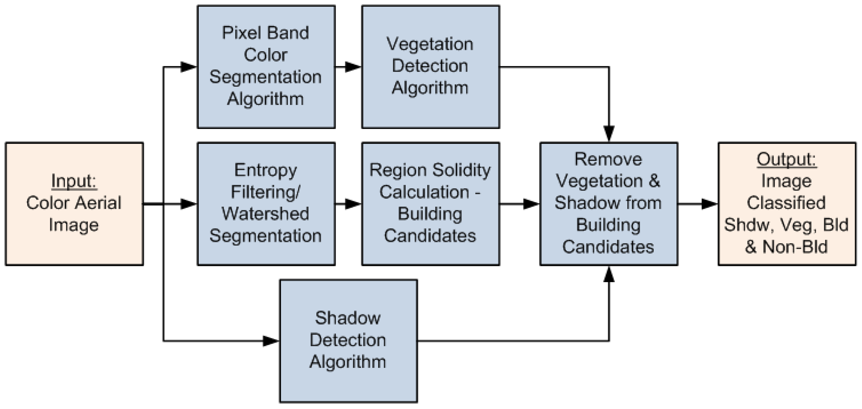
We therefore propose an automated approach to building detection from a single, nadir, color aerial image with making very few assumptions about the buildings being detected. In striving to achieve automatic building detection, we have also come up with an automated approach for detecting vegetation as well from a single nadir, color aerial image. Results are presented for a given data set containing thousands of buildings of varying sizes, roof top colors and shapes. In
Section 2, a detailed description of the proposed approach is presented. In
Section 3, some characteristics about the two different data sets are described, evaluation metrics are discussed and results from the algorithm being tested on the two data sets are presented. In
Section 4 we draw conclusions and future work is presented in
Section 5.
3. Experimental Results
3.1. Empirical Parameters
The entropy image threshold (0.75), the color segmentation bin quantization (17), the region solidity (0.7) and the vegetation region threshold (0.6) were empirically determined by qualitatively examining the visually best results demonstrated on a small subset of the Fairfield data set (five images totaling in size to 7% of the actual dataset). Note, in evaluating the parameter selection, those images were visually examined; the reference set was never consulted during this phase nor were parameter sweeps done. These parameters were then held fixed for the algorithm’s execution across both the Fairfield and Anchorage data sets.
3.2. Data Sets
The proposed algorithm has been tested on two different data sets. The first data set depicts a 2 × 2 km
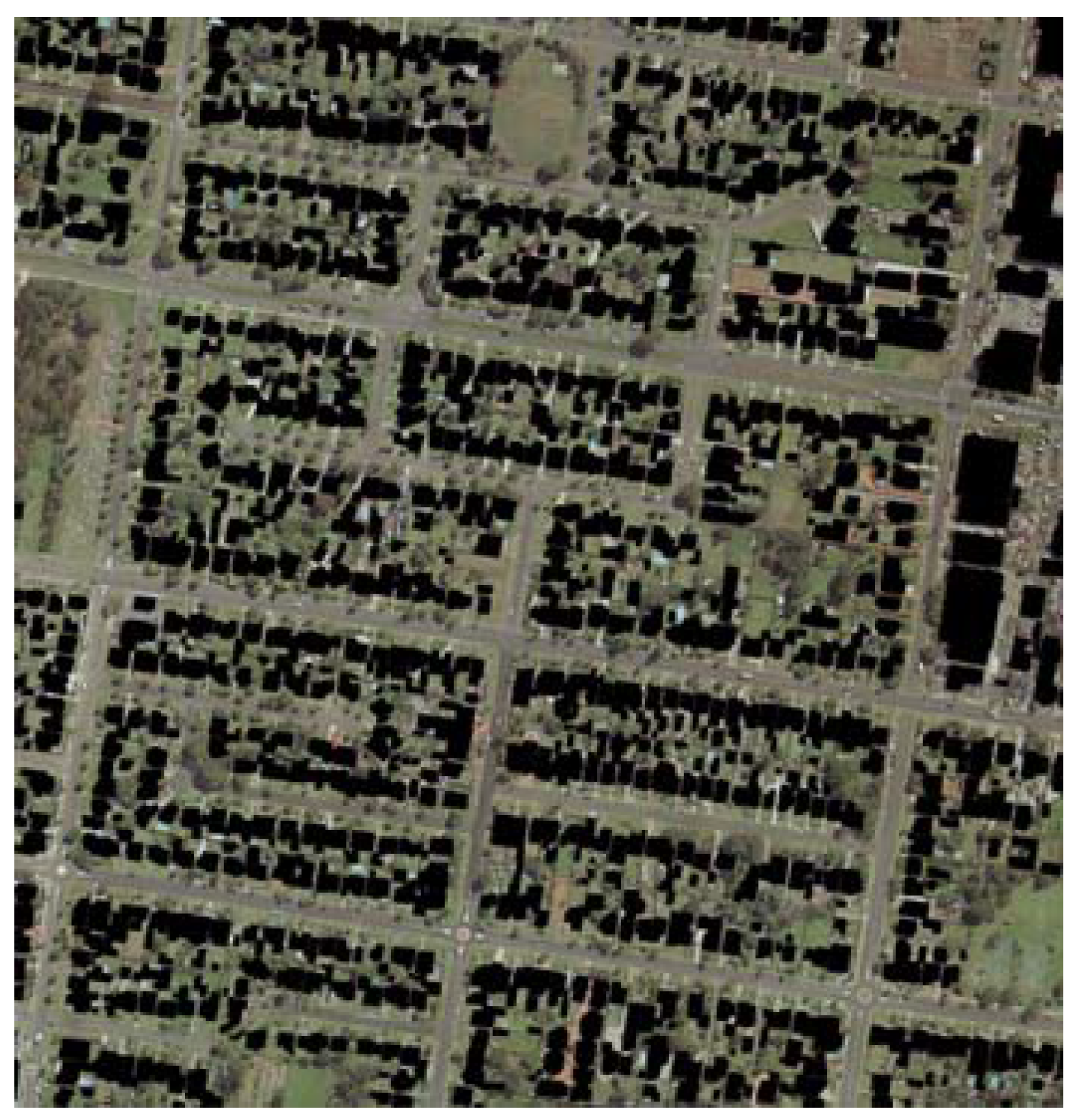
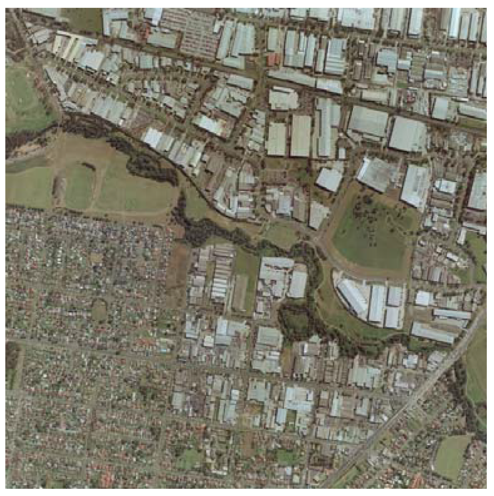
2 area from Fairfield (Australia) and is referred to from here on out as “the Fairfield data set”. This data set includes LiDAR data, containing first and last return pulse information, as well as returned pulse intensity. The data set also has a RGB aerial color image, which is depicted in
Figure 9, having 15 cm pixel resolution. A suburban area exists to the southwest whereas the northeast mostly contains industrial buildings.
Figure 9.
Fairfield Data Set Aerial Imagery.
Figure 9.
Fairfield Data Set Aerial Imagery.
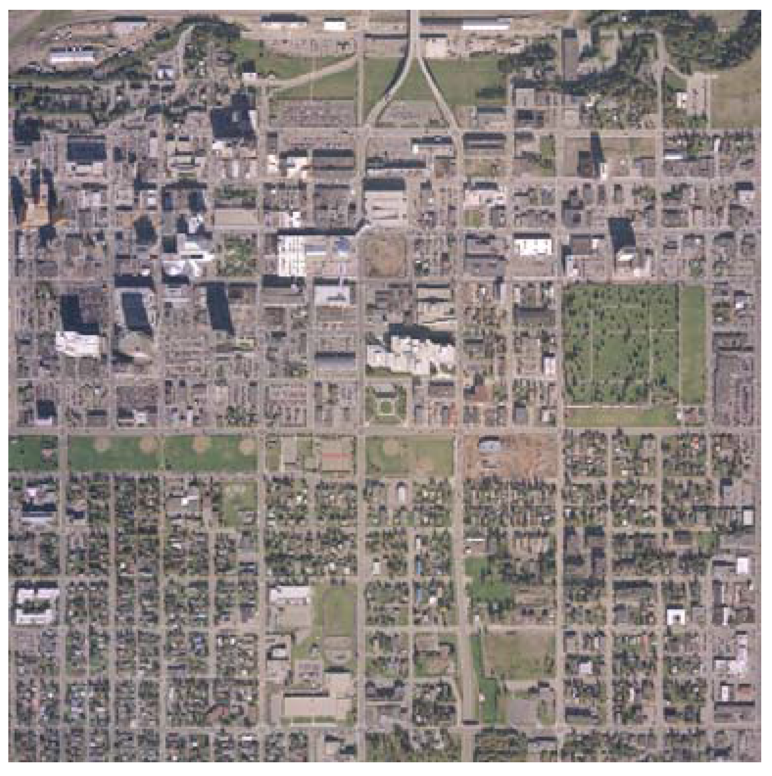
Figure 10.
Anchorage Data Set Aerial Imagery.
Figure 10.
Anchorage Data Set Aerial Imagery.
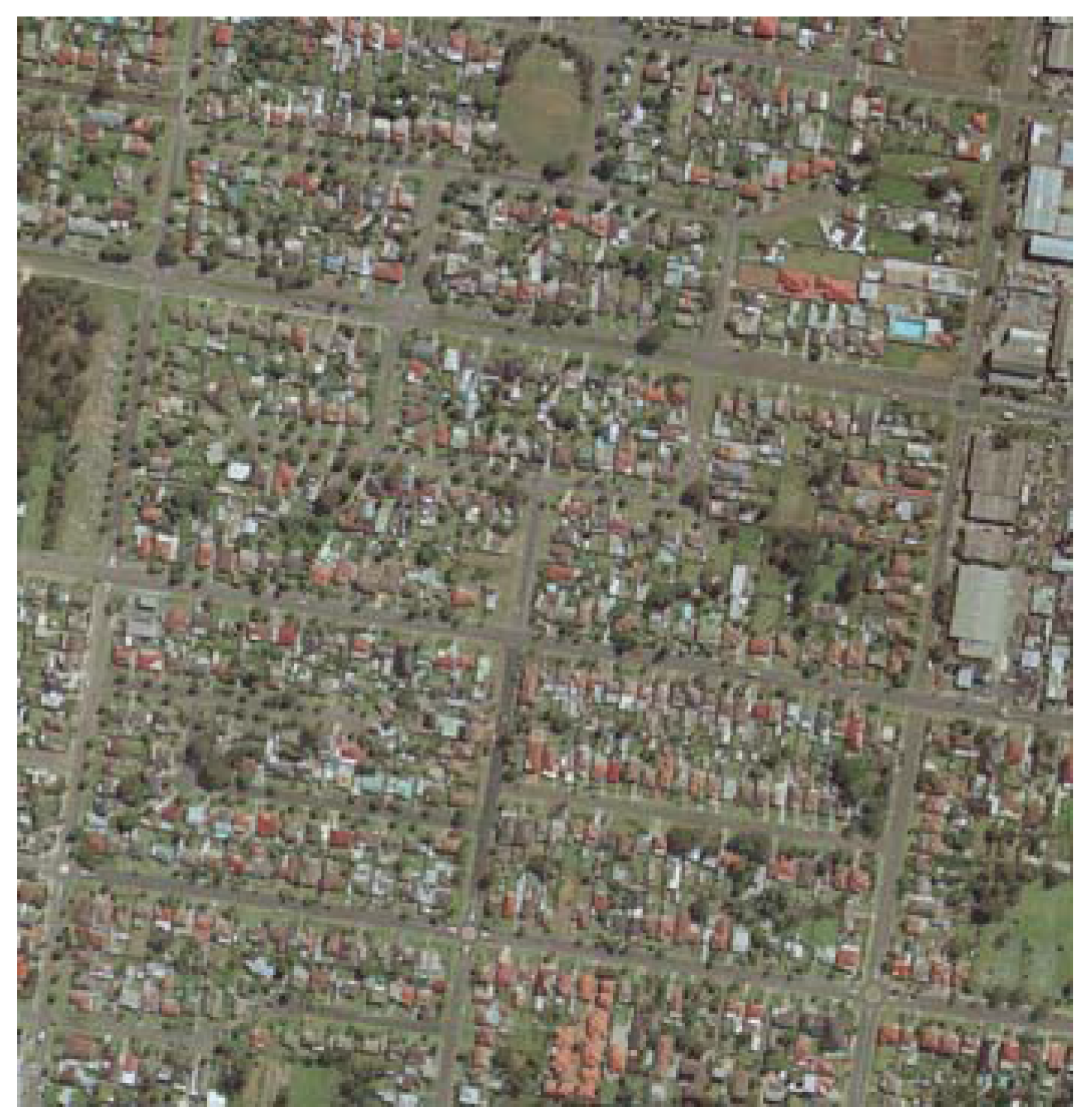
A cropped portion of
Figure 9, showing the residential buildings existent in the south west portion of the data set, is shown in
Figure 11. The manual identification of the buildings in
Figure 11 is shown in
Figure 12.
Figure 11.
Cropped Residential Portion of the Fairfield Data Set Aerial Imagery.
Figure 11.
Cropped Residential Portion of the Fairfield Data Set Aerial Imagery.
Figure 12.
Cropped Residential Portion of the Manually Identified Buildings in Fairfield Data Set.
Figure 12.
Cropped Residential Portion of the Manually Identified Buildings in Fairfield Data Set.
The second data set depicts a 1.67 × 1.67 km
2 area from Anchorage (Alaska, USA) and from here on out is referred to as “the Anchorage data set”. This data set includes both LiDAR data, with first return pulses and no last return nor returned intensity, and aerial imagery, shown in
Figure 10, existing as an RGB color image at 15 cm pixel resolution with a planned horizontal accuracy of 60 cm.
In both data sets, the LiDAR data and the aerial image depict the terrain from a nadir/top down perspective and the accompanying aerial image has been ortho rectified. The Fairfield data set has different building and terrain characteristics when compared to the Anchorage data set. The industrial portion of the Fairfield data set is not by any means equivalent to the commercial portion of the Anchorage data set. The buildings in the industrial portion of the Fairfield data set, for the most part, lie relatively low and have a large base, whereas some of the commercial buildings in the Anchorage data set rise fairly high. Because the sun is lower to the ground when the Anchorage data set was captured, the shadows in the Anchorage are longer than the Fairfield data set. Furthermore, the Anchorage data set to the North East contains a highly populated urban area filled with a great deal of concrete and little vegetation. There is some dense forestry to the North West of the Anchorage data set. Whereas there exists more vegetation in the industrial part of the Fairfield Data Set to the North West (in comparison to the Anchorage data set’s commercial sector) and there’s a dense forestry spanning through the center of the data set.
In order to evaluate the accuracy of the proposed algorithm, building pixels were first manually identified in both data sets. The Fairfield data set contained a total of 1,401 building regions and the Anchorage Data set contained 1,242 building regions. This set of manually labeled points will be referred to as the reference set. The proposed building detection algorithm labels all points belonging to different buildings with unique building labels. From here on out this will be referred to as the automatic set.
3.3. Evaluation Metrics
For evaluating the automatically extracted buildings, using a reference data set, two performance metrics are pertinent—the completeness and the correctness of the results [
20]. On a pixel level, the completeness represents the percentage of pixels belonging to buildings that were correctly detected by the algorithm. The correctness represents the percentage of pixels labeled by the algorithm as building that actually correspond to building points.
On a building level, the completeness represents the percentage of buildings that are correctly detected by the algorithm and the correctness represents the percentage of buildings that the algorithm identified that are actually buildings which exist in the reference set. The building level completeness and correctness metrics used in this research are calculated the same way in which they are defined by Rottensteiner
et al. in Section 3.2 of [
2] which were also used in [
3].
3.4. Building Detection Results: Pixel and Building Level Completeness and Correctness
The pixel level completeness and pixel level correctness achieved by the proposed building detection algorithm for the Fairfield data set are 0.8258 and 0.6163, respectively. This means that 82.6% of the pixels belonging to buildings, according to the reference set, were correctly detected by the algorithm in the automatic set and that 61.6% of the pixels labeled as building by the algorithm in the automatic set were actually also labeled building in the reference set. The pixel level completeness and pixel level correctness for the Anchorage data set are 0.7486 and 0.4154, respectively. Again, 74.9% of the pixels belong to buildings were correctly detected by the algorithm and 41.5% of the pixels labeled as building by the algorithm actually corresponded to building pixels. Confusion matrices for the results from both data sets are shown in
Table 1 and
Table 2. The algorithm realized a kappa value of 0.5613 on the Fairfield Data set and 0.34109 for the Anchorage Data set.
Table 1.
Confusion Matrix for Fairfield Data Set.
Table 1.
Confusion Matrix for Fairfield Data Set.
| | | Auto |
|---|
| | | Bld | Non-Bld |
|---|
| Ref | Bld | 42,279,727 | 8,920,741 |
| Non-Bld | 26,321,752 | 100,433,380 |
Table 2.
Confusion Matrix for Anchorage Data Set.
Table 2.
Confusion Matrix for Anchorage Data Set.
| | | Auto |
|---|
| | | Bld | Non-Bld |
|---|
| Ref | Bld | 20,260,940 | 6,803,900 |
| Non-Bld | 28,515,278 | 63,142,698 |
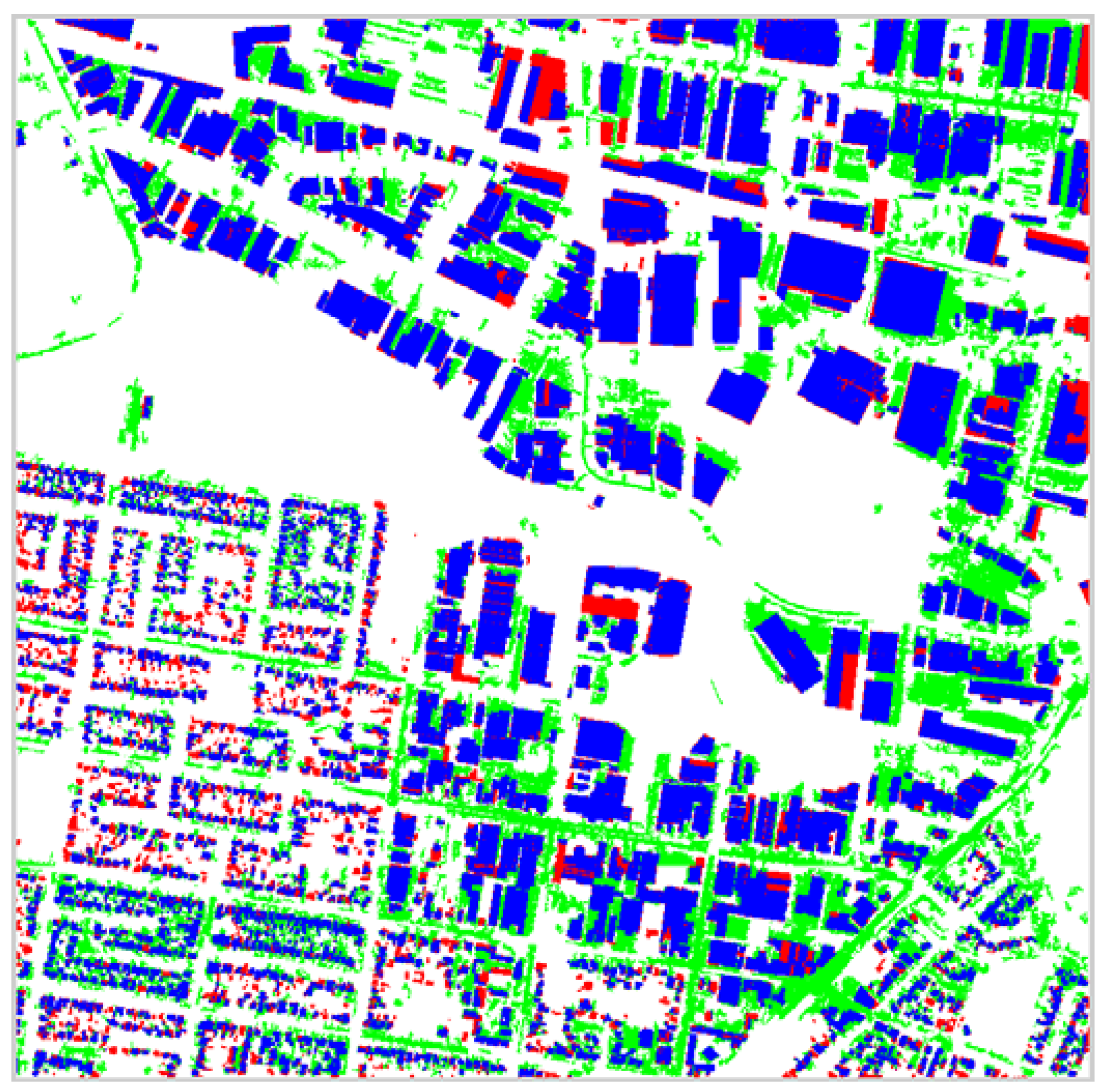
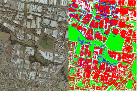
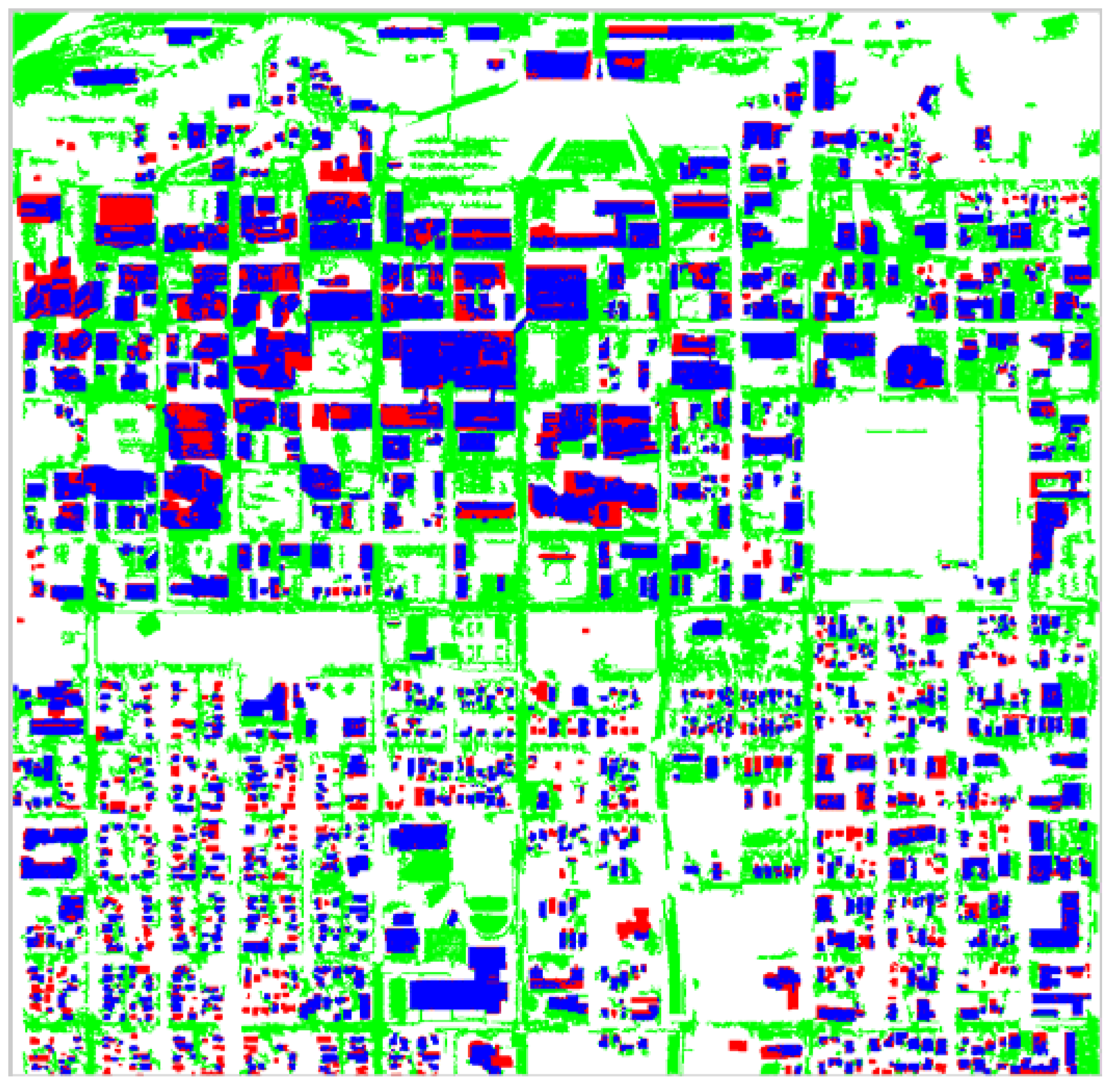
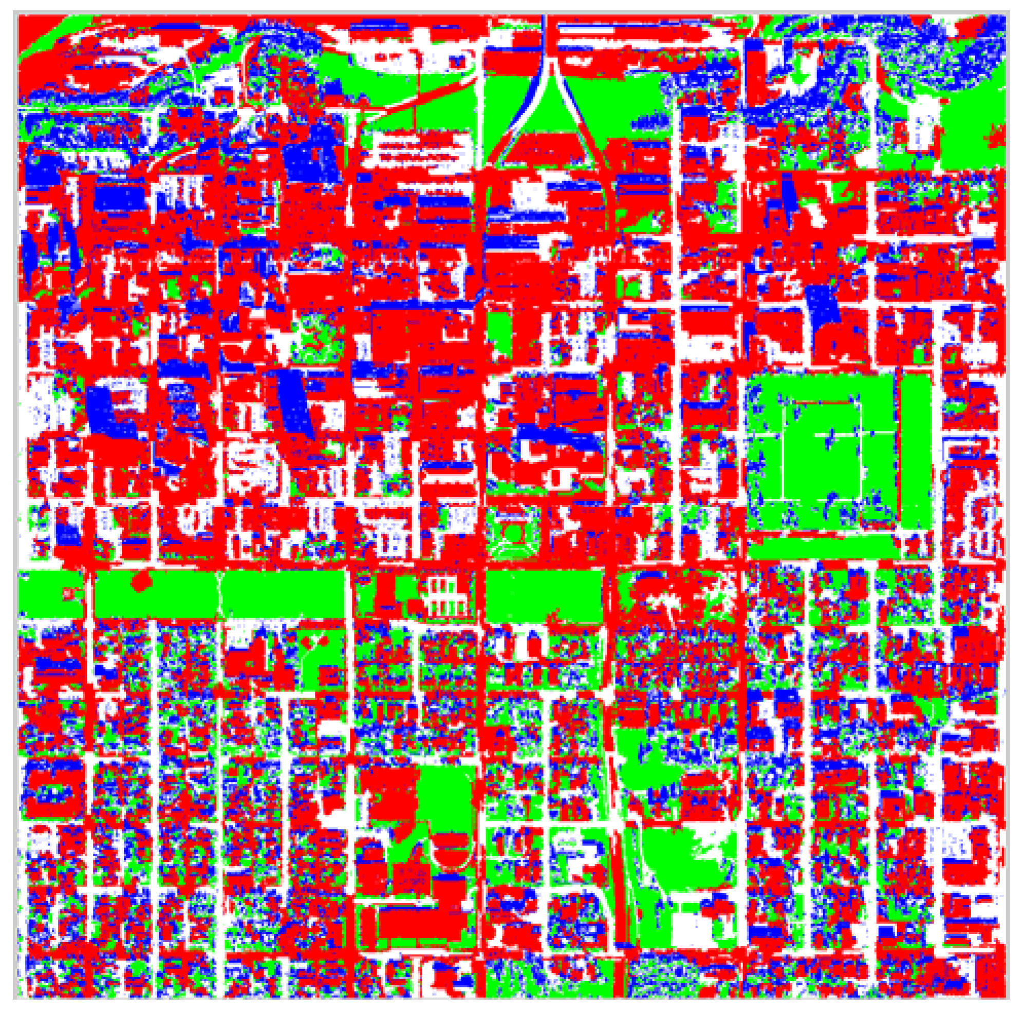
Figure 13 and
Figure 14 presents pixel level results for the entire Anchorage and Fairfield data sets respectively. In these figures, the blue color corresponds to correctly detected points, the light green color corresponds to false positives (points the algorithm classified as belonging to buildings in the automatic set but were in fact identified as not belonging to buildings in the reference set) and the red color corresponds to false negatives (points that were identified as belonging to buildings in the reference set but classified as not belonging buildings in the automatic set by the algorithm). The white in these figures corresponds to points not identified as building by both the algorithm in the automatic set and the manual extraction in the reference set (true negatives).
Observe that in
Figure 13 and
Figure 14 almost all of the false positive pixels correspond to either roads, sidewalks, parking lots, or dirt. Some of the roads have been correctly classified as non-building because their solidity is too low when represented by a single segment. The majority of the false negatives are smaller buildings or are due to buildings casting shadows on other buildings. The algorithm performs very well in not mistaking vegetation for building.
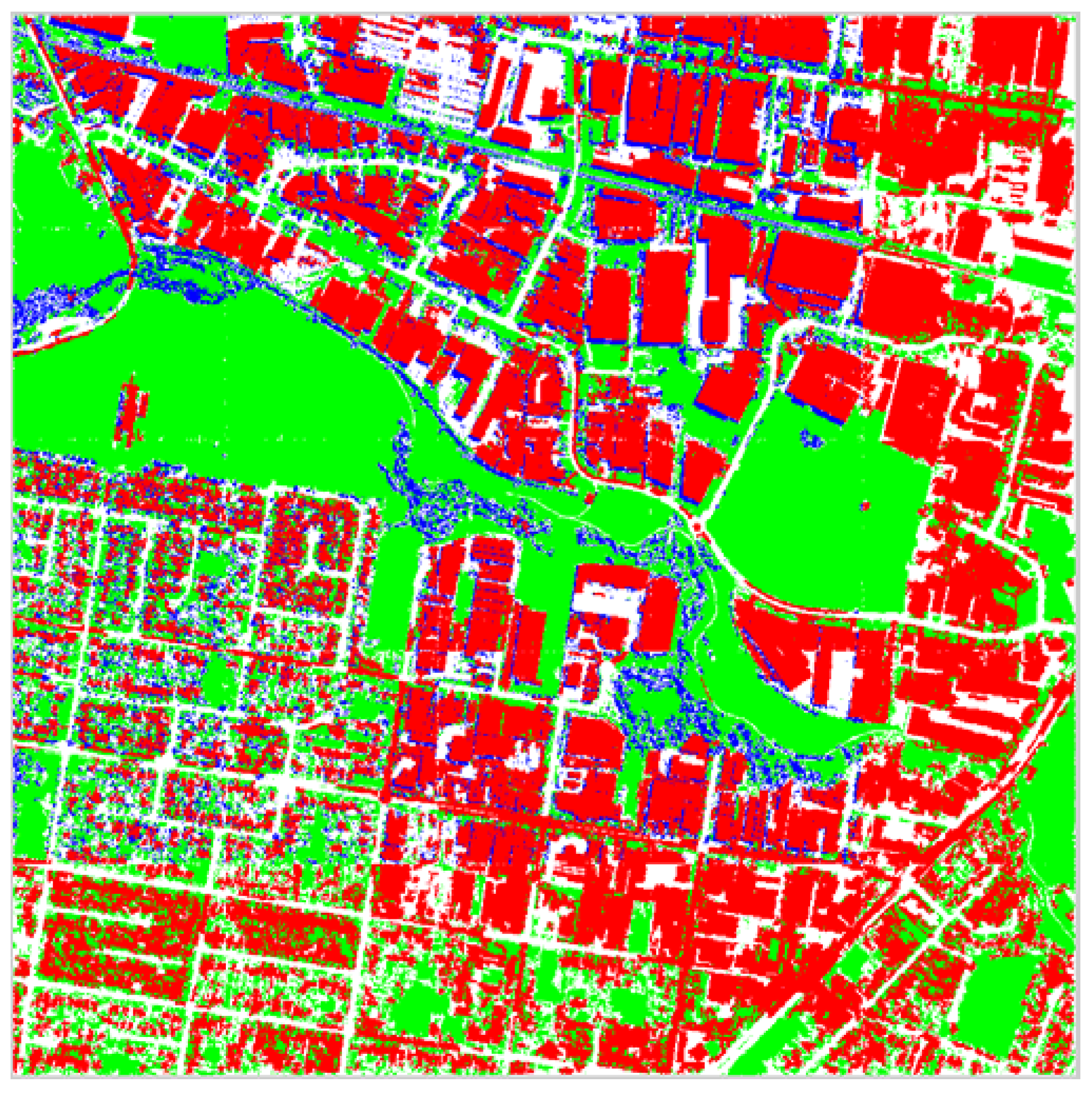
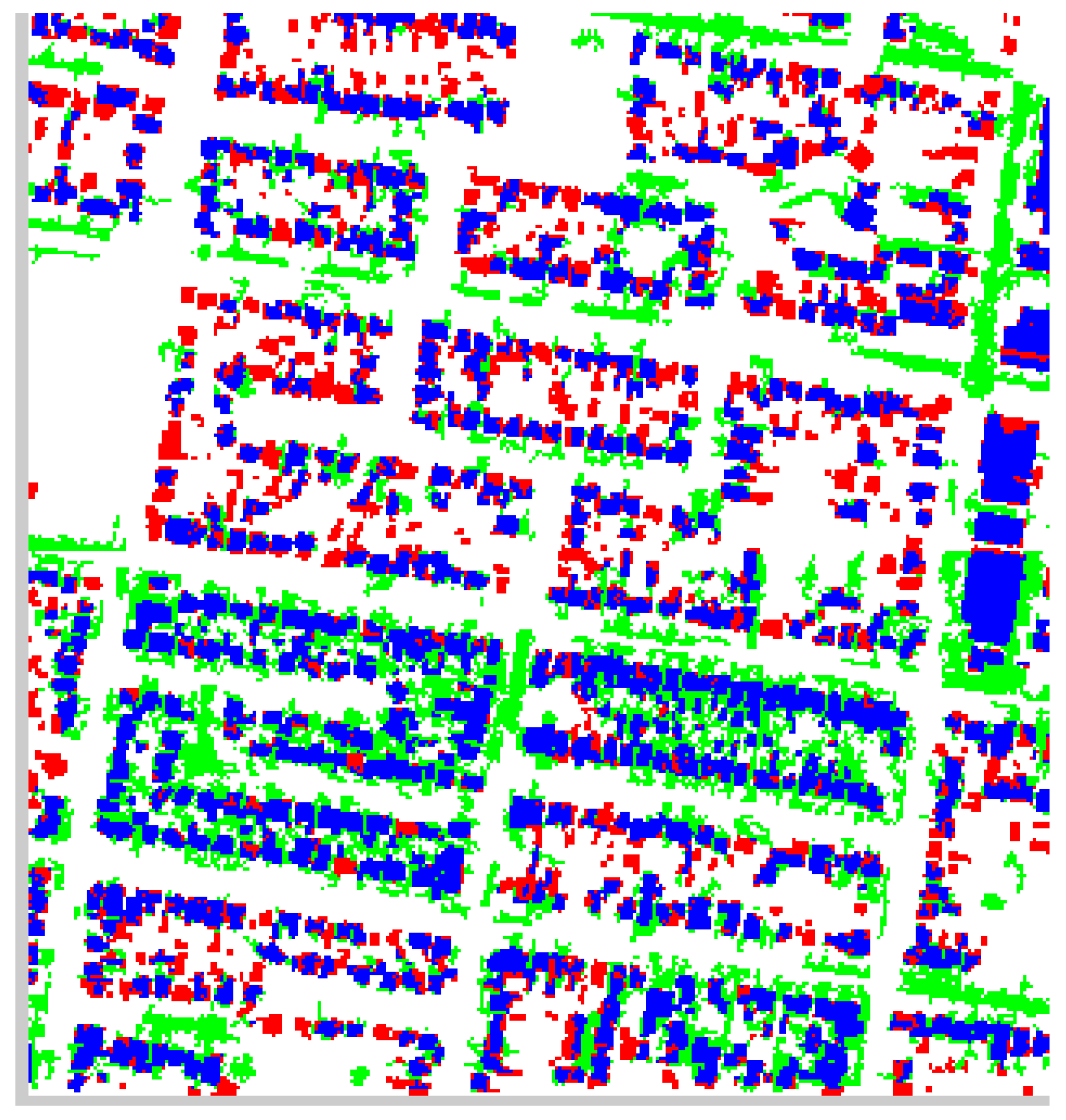
Figure 15 and
Figure 16 present pixel classification results as buildings, non-buildings, shadow and vegetation for entire the Anchorage and Fairfield data sets respectively. The red pixels correspond to what the proposed algorithm classified as building, the green pixels as vegetation, the blue pixels as shadow and the white pixels as non-building. Unfortunately, the darker side of trees is often classified as shadow, which is correct however the trees typically overcast vegetation. Most of the non-building correctly corresponds to concrete surfaces such as roads or parking lots, which are not parts of buildings. Again, observe that the algorithm performs very well in identifying the sun side part of the dense forestry and the rest of the vegetation existent in the data set.
Figure 13.
Building Pixel Accuracy for the Anchorage Data Set.
Figure 13.
Building Pixel Accuracy for the Anchorage Data Set.
Figure 14.
Building Pixel Accuracy for the Fairfield Data Set.
Figure 14.
Building Pixel Accuracy for the Fairfield Data Set.
Figure 15.
Pixel Classification for Anchorage Data Set.
Figure 15.
Pixel Classification for Anchorage Data Set.
Figure 16.
Pixel Classification for Fairfield Data Set.
Figure 16.
Pixel Classification for Fairfield Data Set.
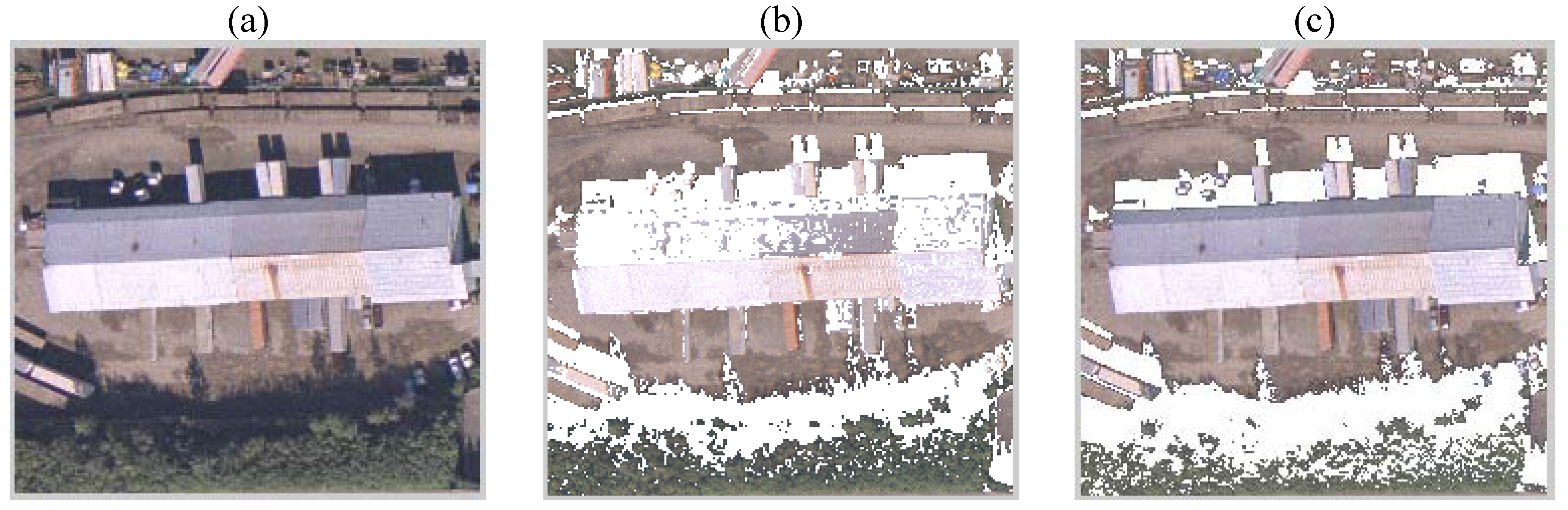
Figure 17 and
Figure 18 present pixel level results for a cropped residential portion of the Fairfield data set.
Figure 17.
Cropped Residential Portion of the Building Pixel Accuracy for the Fairfield Data Set.
Figure 17.
Cropped Residential Portion of the Building Pixel Accuracy for the Fairfield Data Set.
Figure 18.
Cropped Residential Portion of the Pixel Classification for Fairfield Data Set.
Figure 18.
Cropped Residential Portion of the Pixel Classification for Fairfield Data Set.
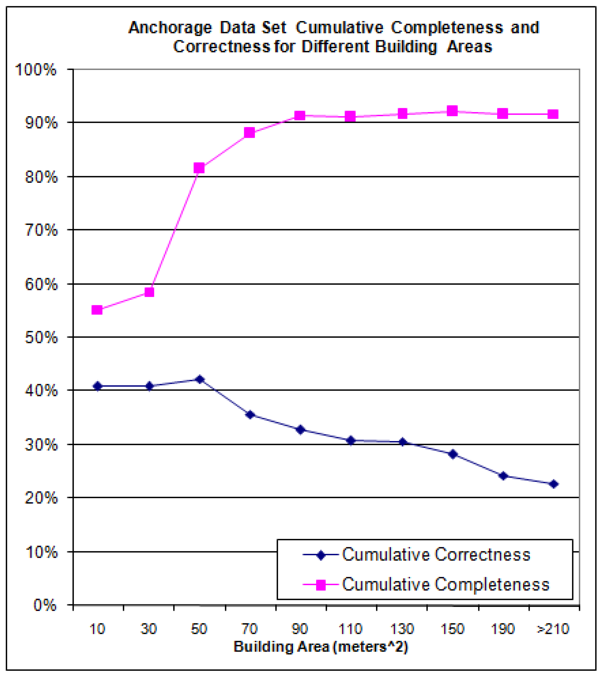
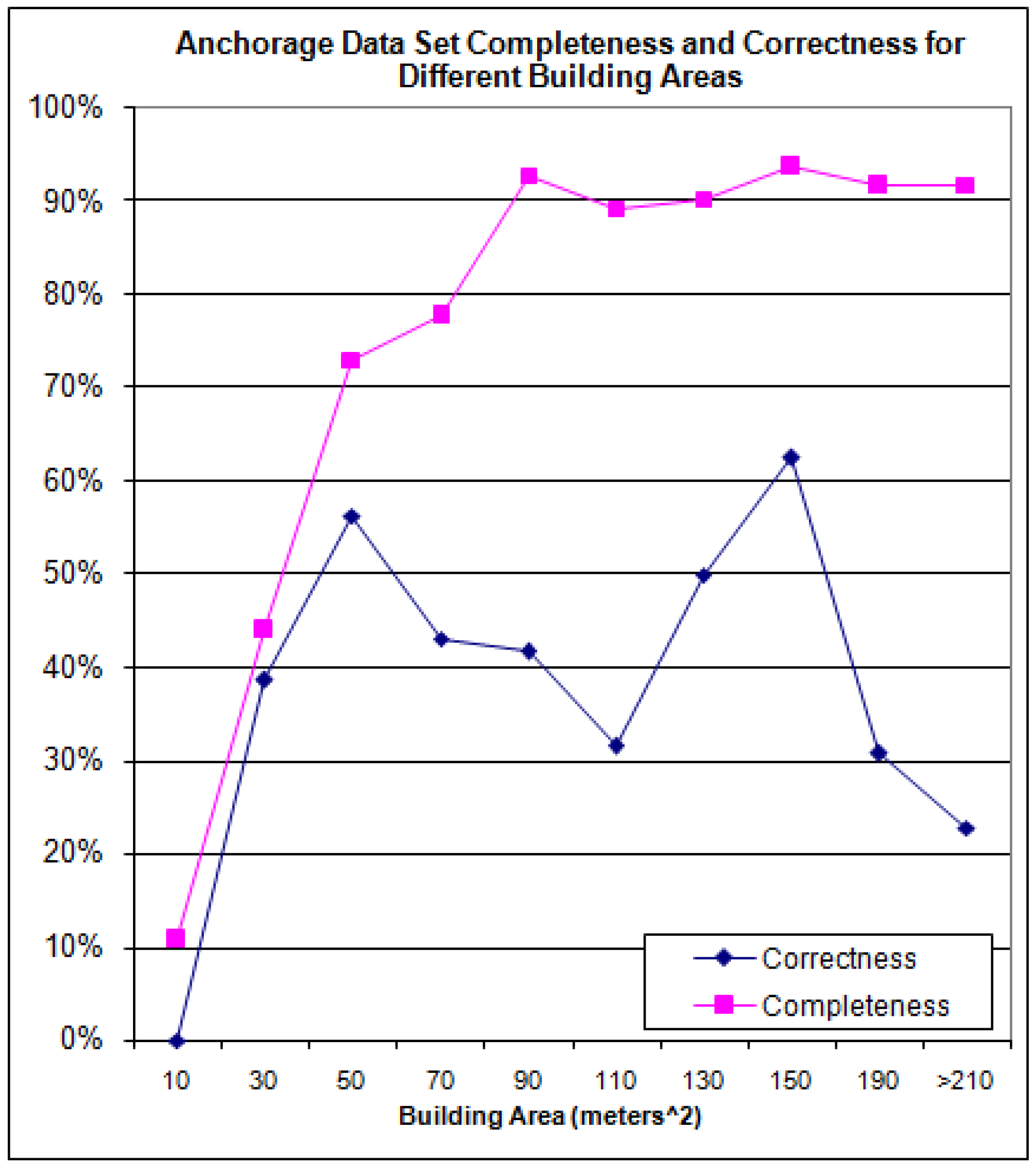
The building level completeness and correctness results, as a function of various building areas, for the Anchorage data set are shown in
Figure 19.
Figure 20 presents cumulative completeness and correctness which is simply the algorithm’s completeness and correctness for all buildings having an area greater than the value shown on the x-axis.
Figure 19.
Completeness and Correctness for the Anchorage Data Set.
Figure 19.
Completeness and Correctness for the Anchorage Data Set.
Figure 20.
Cumulative Completeness and Correctness for the Anchorage Data Set.
Figure 20.
Cumulative Completeness and Correctness for the Anchorage Data Set.
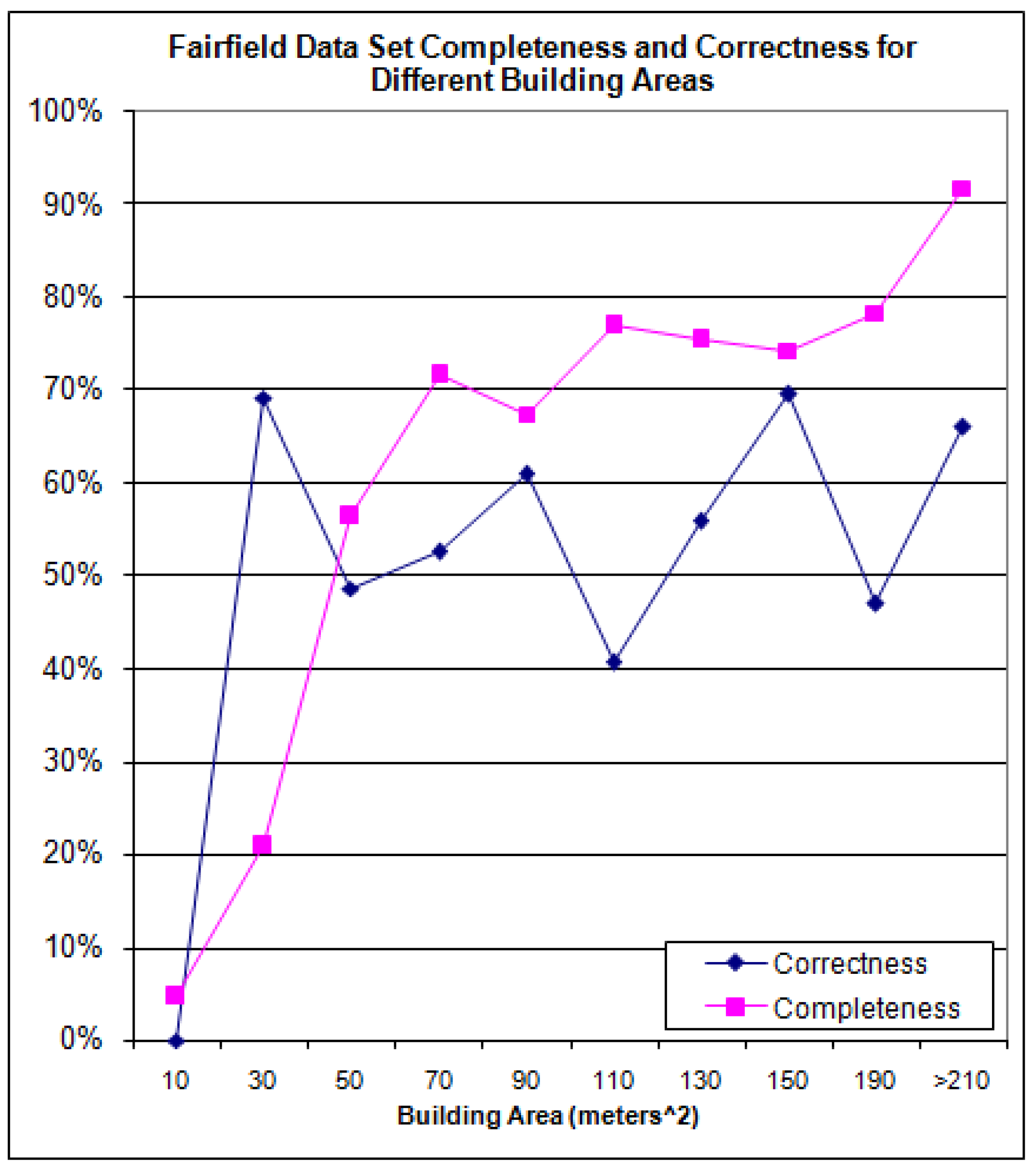
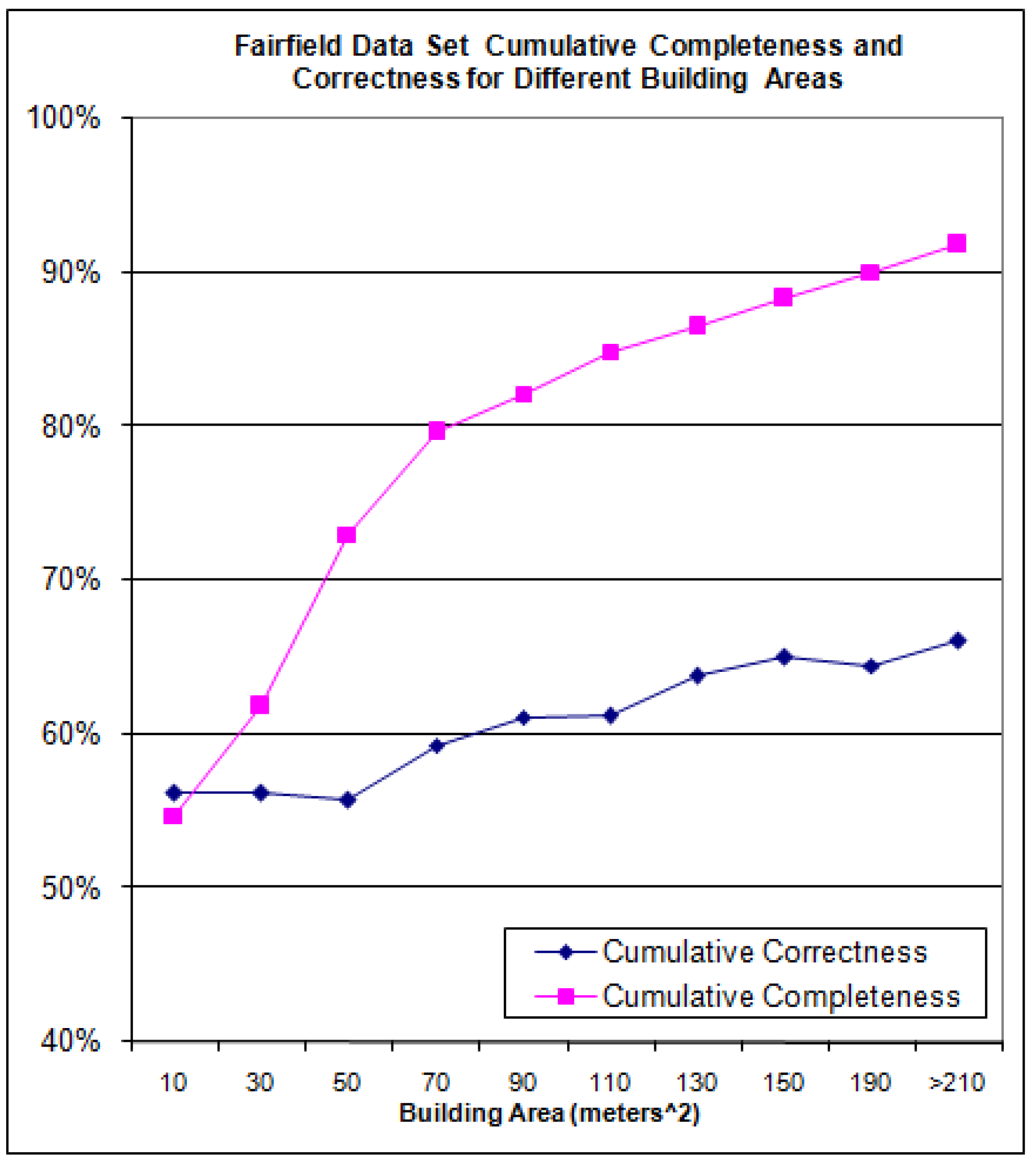
The building level completeness and correctness for the Fairfield data set is shown in
Figure 21 and the cumulative completeness and correctness in
Figure 22.
Figure 21.
Completeness and Correctness for the Fairfield Data Set.
Figure 21.
Completeness and Correctness for the Fairfield Data Set.
Figure 22.
Cumulative Completeness and Correctness for the Fairfield Data Set.
Figure 22.
Cumulative Completeness and Correctness for the Fairfield Data Set.
In
Figure 22 note that for a building area of 150 m
2 for the Fairfield data set, the algorithm has a cumulative completeness and cumulative correctness of approximately 88% and 65%, respectively. This simply means that the algorithm’s completeness and correctness for all buildings having an area of 150 m
2 and greater is 88% and 65% (respectively). The range was plotted from between 10 m
2 to 210 m
2 as after 210 m
2. The algorithm detects 80% of the buildings larger than 70 m
2 but at the same time its correctness suffers at the expense of false positives. The reason for the mediocre correctness is the algorithm is completely automated: no parameters change during the execution across the data sets. Also, no assumptions are implemented to tailor to a specific building size or shape. As it is shown soon via the data set building histogram, there are a variety of different building sizes in the data set. Finally, the mediocre correctness is also because the automatic algorithm is detecting these buildings from only a single nadir aerial image.
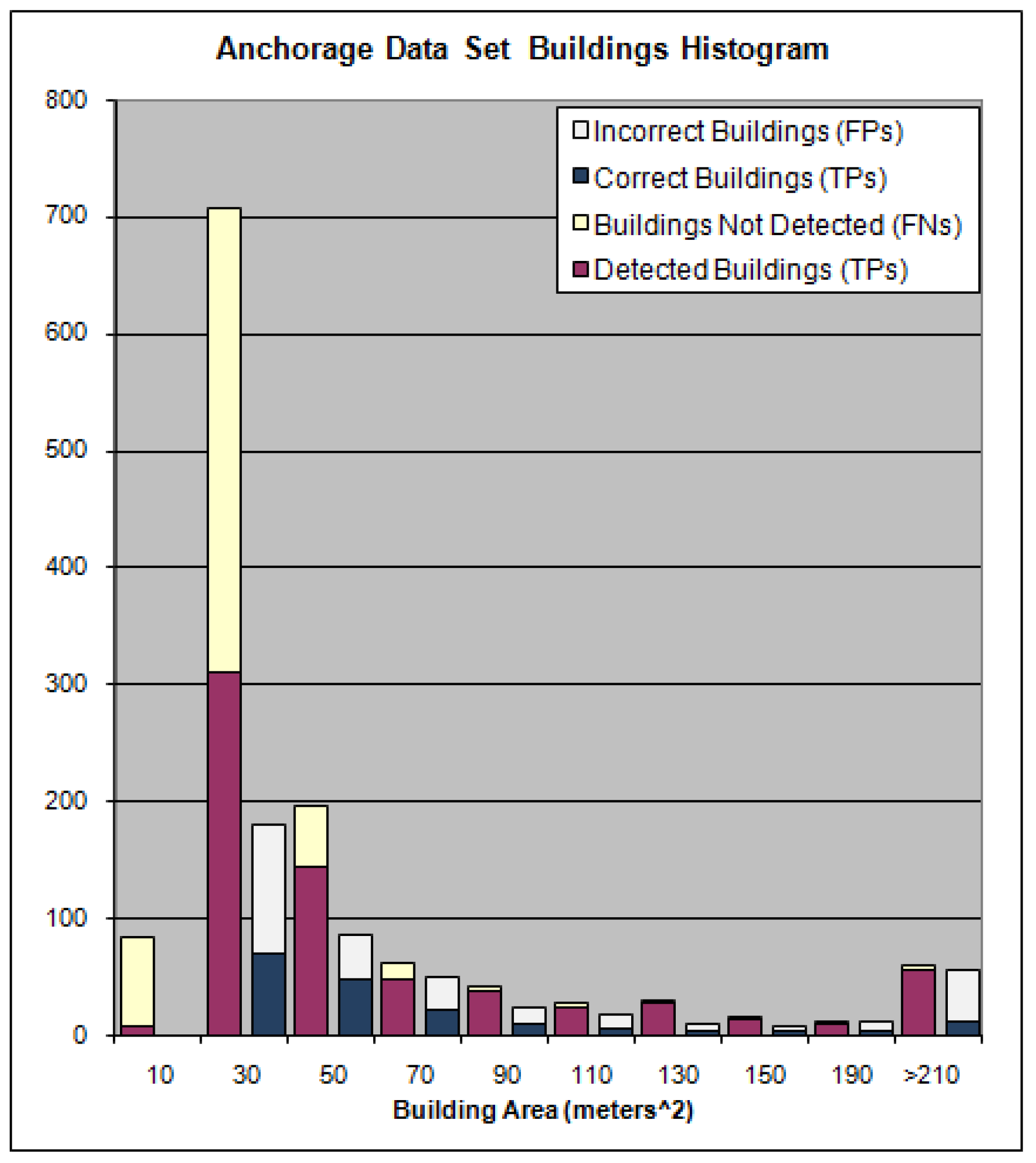
The histogram for building sizes the Anchorage data set is shown in
Figure 23 and for the Fairfield data set in
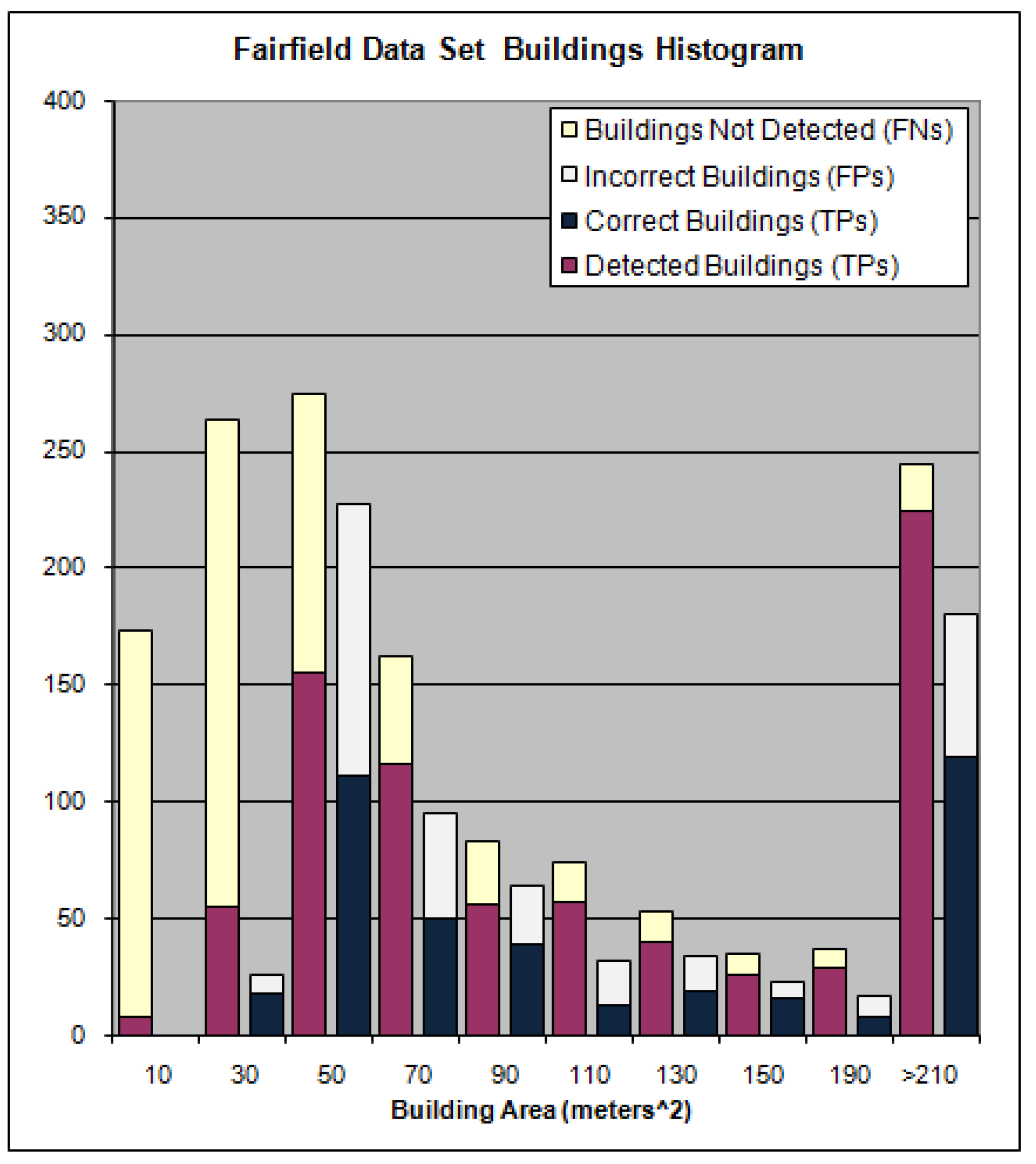
Figure 24. The height of the red and yellow bars represent the total number of buildings manually extracted for the building area listed on the x–axis. The height of the blue and gray bars represent the total number of buildings identified by the algorithm for the building area listed on the x–axis. The red part of the red and yellow bar is proportional to the amount of those buildings which were detected by the algorithm whereas the yellow portion of the bar represents the buildings the algorithm failed to detect for the given area on the x–axis. The blue portion of the blue and gray bars represents the number of buildings the algorithm detected which actually corresponded to buildings in the reference set and the gray portion represents the number of buildings the algorithm claimed to be building but did not correspond to any buildings identified in the reference set for the building area listed on the x–axis.
Figure 23.
Anchorage Data Set Histogram.
Figure 23.
Anchorage Data Set Histogram.
Figure 24.
Fairfield Data Set Histogram.
Figure 24.
Fairfield Data Set Histogram.
3.5. Vegetation Detection Results: Pixel Correctness and Percent Coverage
We mentioned earlier that for the Fairfield data set there is also LiDAR data because it is possible to use the returned LiDAR intensity and one of the channels from the aerial image to compute a pseudo normalized difference vegetation index (NDVI) and threshold that NDVI image to identify vegetation. Rottensteiner
et al. in [
3] propose using the pseudo NDVI image calculate it by taking the difference of the returned LiDAR intensity at pixel (i,j) and the red color component for that same pixel (from the RGB image) and divide that quantity by the sum of the returned LiDAR intensity and the red color component of the pixel. Note that in order to use the NDVI image, the LiDAR data must be interpolated and registered to the aerial imagery so that the LiDAR intensity at pixel (i,j) and the red color component at (i,j) correspond to the same location in the depicted scene.
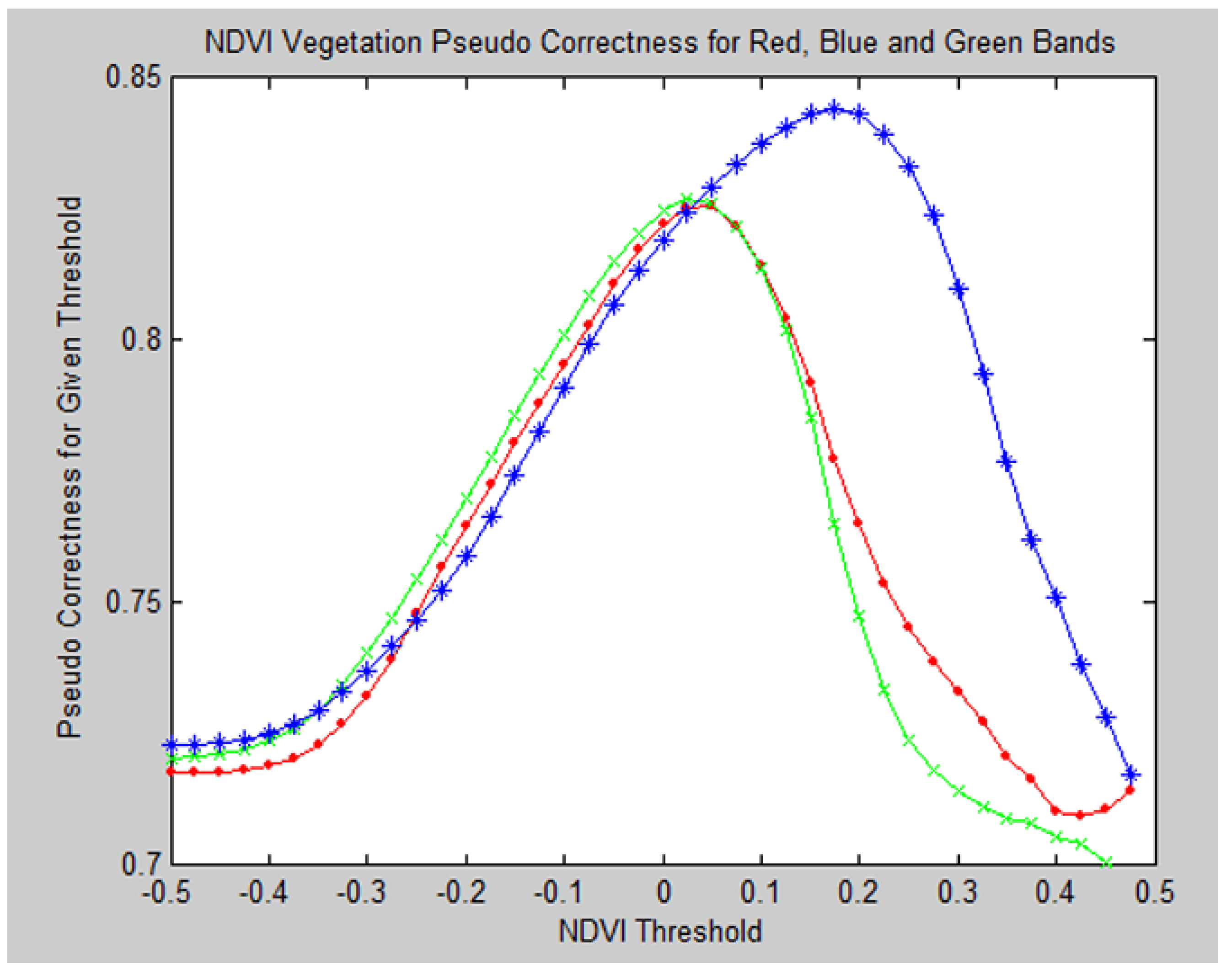
With the manually developed reference set, we know which pixels belong to buildings and which do not. We then tried 40 different thresholds (for thresholding the pseudo NDVI image to determine where vegetation exists). The thresholds ranged from −0.5 to 0.5 in increments of 0.025. We then calculated the pseudo correctness for the red, blue and green channel based NDVI images for all the thresholds and plotted the accuracy. The pseudo correctness is calculated as follows:
In equation (8) pTP is Pseudo True positive and FP is a false positive. If the thresholded NDVI labels a pixel as vegetation and that corresponding pixel is not labeled as belonging to a building in the reference set, then the pixel is classified as a pseudo true positive. The reason this is referred to as a ‘pseudo’ true positive’ is because what is not building could be sidewalk, cement, etc. in addition to vegetation. A reference set was only developed for identifying buildings, not vegetation. If the thresholded NDVI labels a pixel as vegetation and that corresponding pixel is also labeled as belonging to a building in the reference set, then the pixel is classified as a false positive.
Because a reference set was not developed which identified the vegetation as ground truth, false negatives cannot be calculated. False negative pixels are pixels in which the thresholded NDVI classifies as not belonging to vegetation when in fact they do belong to vegetation. Instead only false positives can accurately be determined. Now, although in [
3] Rottensteiner use the red channel, in earlier works [
21], they report using the green channel of the aerial imagery.
Figure 25 shows the pseudo correctness plotted for the red, green and blue thresholded NDVI images for all thresholds tested. In
Figure 25, the red line corresponds to the NDVI constructed from the returned LiDAR intensity and the red channel of the corresponding color aerial imagery (similarly for the green and blue channels for the green and blue lines).
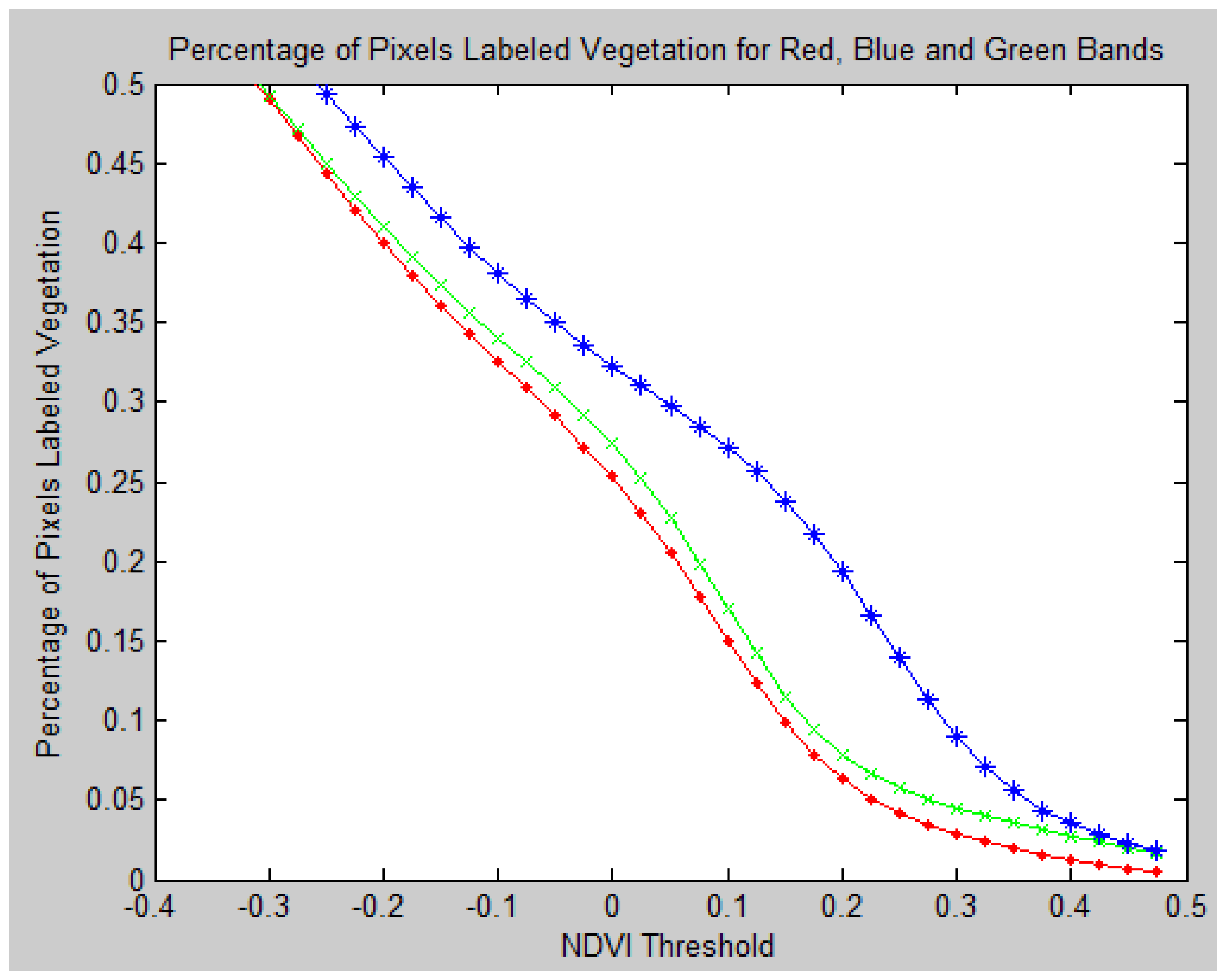
Figure 25 shows the percentage of pixels classified as vegetation by the pseudo NDVI approach.
We tested our proposed color invariant vegetation detection approach on the Fairfield Data Set and the Anchorage Data Set and it realized a pseudo correctness of 97.25% and 96.91%, respectively. Note that our approach only requires the aerial imagery and is automatic—no parameter adjustment. A comparison of the best NDVI results and ours are presented in
Table 3 where our method is listed as ‘Clr Inv Veg’ and the best results from thresholding the different channel NDVI images are listed as ‘NDVI Red’, ‘NDVI Blue’ and ‘NDVI Green’. Not only does our approach realize a significantly higher correctness, but it is also labeling more pixels as vegetation than the thresholding of the NDVI images.
Figure 25.
Pseudo Correctness for R, B and G Channel Based NDVI Veg. Identification.
Figure 25.
Pseudo Correctness for R, B and G Channel Based NDVI Veg. Identification.
Figure 26.
Percentage of Pixels labeled Veg. for Red, Blue and Green Channel Based.
Figure 26.
Percentage of Pixels labeled Veg. for Red, Blue and Green Channel Based.
Table 3.
Correctness and Coverage Comparison.
Table 3.
Correctness and Coverage Comparison.
| Method | Correctness | Coverage | Data Set |
|---|
| NDVI Red | 82.55% | 20.56% | Fairfield |
| NDVI Green | 82.71% | 25.23% | Fairfield |
| NDVI Blue | 84.39% | 21.67% | Fairfield |
| Clr Inv Veg | 97.25% | 30.05% | Fairfield |
| Clr Inv Veg | 96.91% | 17.88% | Anchorage |
3.6. Building Detection Comparison with Other Surveyed Methods
Several approaches in the literature only benchmark their algorithm on less than 250 buildings. The only approach we found tested on more than 250 buildings and reported their building completeness realized a 63.60%. All of the approaches surveyed either didn’t report their pixel or their building level correctness; we are the only ones to report both. We have provided in
Table 4 a comparison of all the approaches surveyed. The characteristics listed for each approach are “Pix Comp”, “Pix Corr”, “Bld Comp”, “Bld Corr”, “# Bldings”, “Resolution”, and “Color/Pan” which corresponds to pixel level completeness, pixel level correctness, building completeness, building correctness, the number of buildings the results were based upon, the resolution of the image the algorithm was tested on, and whether that image was panchromatic or color, respectively. The approaches compared are Lefevere
et al. [
7], Muller
et al. [
8], Persson
et al. [
9], Sirmacek
et al. [
10], Liu
et al. [
13], and Benediktsson
et al. [
14]. Also our approach for all buildings (“Shorter all”), then our approach for buildings having an area of 50 m
2 and greater (Shorter 50), and finally our approach for buildings having an area of 210 m
2 and greater (Shorter 210), is also provided. The cells with ‘X’s correspond to data that was not available or not reported. No definitive conclusions are drawn as the data sets used by other authors were different than the data sets we used.
Table 4.
Completeness/Correctness at Pixel and Building Level for various Approaches.
Table 4.
Completeness/Correctness at Pixel and Building Level for various Approaches.
| Approach | Pix Comp | Pix Corr | Bld Com | Bld Corr | #Bldings | Resolution | Color/Pan |
|---|
| Lefevre | 63.6% | 79.4% | X | X | X | 70 cm | Pan |
| Muller | 77.3% | 79.5% | X | X | 240 | 30 cm | RGB |
| Persson | 53.0% | 93.0% | 82.0% | X | 17 | 25 cm | RGB |
| Sirmacek | X | X | 86.6% | X | 177 | 30 cm | RGB |
| Liu | X | X | 94.5% | 83.4% | 277 | 60 cm | RGB |
| Benediktsson | 80%,95.1% | X | X | X | 8952,17319 | 1 m, 5 m | Pan, Pan |
| Shorter all | 78.7% | 51.6% | 55.4% | 48.2% | 2643 | 15 cm | RGB |
| Shorter 50 | X | X | 77.3% | 64.4% | 1414 | 15 cm | RGB |
| Shorter 210 | X | X | 91.8% | 44.5% | 306 | 15 cm | RGB |
4. Conclusions
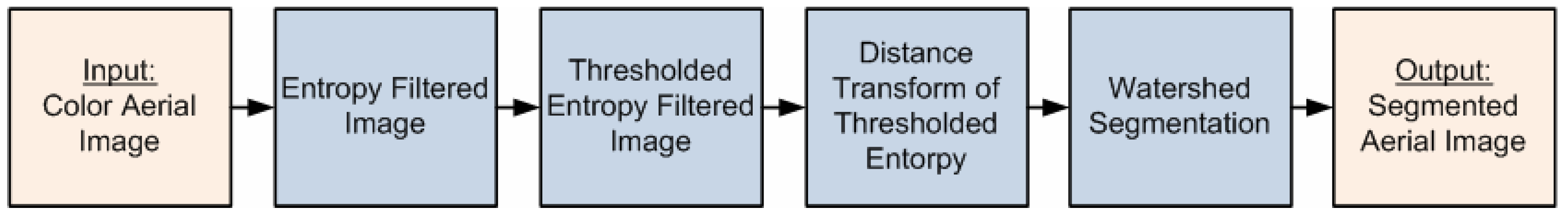
A new method for object classification from a single nadir aerial image is presented. The proposed method uses a novel color quantization technique coupled with a color invariant scheme to identify vegetation. A novel shadow detection procedure is proposed. We use the distance transform coupled with a thresholded entropy filtered image and watershed segmentation to realize entropy segmentation. We then propose the use of solidity as a metric to identify building regions from the entropy segmentation technique. We implemented the proposed method using Matlab and executed the algorithm on an Intel Core 2 Duo (3.0 GHz) machine. The Fairfield data set is a 13,340 × 13,340 pixel image and the Anchorage a 10,896 × 10,896 pixel image. It took the algorithm 90 minutes to complete its execution on the Fairfield data set and 55 minutes for the Anchorage data set.
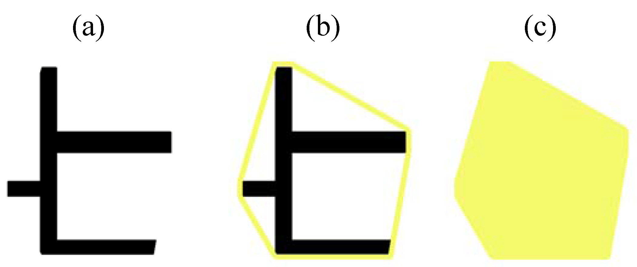
The method has several advantages which make it attractive for unsupervised building detection from aerial imagery. One important feature is the algorithm is automatic, meaning that there is no user input or parameter adjustment. The only assumptions employed by the algorithm in regards to building structures are that no shadows are cast upon the tops of buildings and that the building rooftop segments exist as convex hulls. The limited assumptions made about buildings enable the proposed algorithm to detect a variety of buildings exhibiting different spectral and structural characteristics. The algorithm is a tertiary classifier capable of classifying objects as non-building and shadow (which shadow assumed to be non-building), building, and vegetation. The proposed vegetation detection realizes approximately 97% correctness on accurately identifying non-building pixels (as building and vegetation are mutually exclusive classes) across two different data sets. The method only requires a single nadir aerial image for its input. Experiments with real data and comparisons with other proposed methods have shown that the proposed algorithm has competitive performance, despite being completely unsupervised while not implementing overly restricting assumptions about building structures (such as buildings having only red roof tops or having rectangular exteriors).
The proposed method has some weaknesses as well. Due to the fact that the method is automatic, works off of only a single nadir aerial image, and does not make overly restricting assumptions about building structures, its correctness measure is mediocre. However, it should be noted it is difficult to comparatively rate the correctness measure, both on the pixel and building level as all methods surveyed in this paper only reported one or the other but not both.


