LaVegMod v2: Modeling Coastal Vegetation Dynamics in Response to Proposed Coastal Restoration and Protection Projects in Louisiana, USA

Abstract

We have developed a computer model of plant community dynamics for Louisiana’s coastal wetland ecosystems. The model was improved as a part of the Louisiana Coastal Master Plan of 2017 and is one of several linked models used to evaluate the potential effects of climate change and sea levels rise as well as the potential effects of alternative approaches to managing the region’s natural resources to mitigate the effects of sea level rise. The model we describe here incorporates a number of improvements over the previous version of the model developed for the 2012 Master Plan, including an expansion of the number of species and habitat types represented, the inclusion of bottomland forests and barrier islands, and the incorporation of additional ecological processes such as dispersal. Here, we present results from the model used to evaluate large scale ecosystem restoration projects, as well as three alternative management scenarios to illustrate the utility of the model and the ability of current management plans to address the threats that sea level rise pose to Louisiana’s coastal wetland ecosystems.

1. Introduction

Louisiana’s coastal ecosystem has been losing land area at an average rate of 87 km²/year from the 1930’s to 2000; amounting to a cumulative loss of more than 25% of land area over that time period [1,2]. Current projections estimate that there will be another 1329 km² of land lost from the ecosystem by 2050 [2]. The lost land supported a number of habitats, including fresh, intermediate, brackish and saline wetlands, and swamp forest. These habitats have been converted into open water habitat. The rapid loss is a significant problem for both the health of the ecosystem, its constituent habitats, and for the human population that depends on the ecosystem for services, including protection of tidal surge, commercial fishing, commerce, and agriculture [3]. Louisiana’s wetlands are a critical part of one of the three major North American flyways for migratory birds [4,5], and are host to a diverse collection of plants and animals.

The conversion of wetland ecosystems into open water has been driven by both local human modification of the landscape in and around the coastal area, and by climate change and sea level rise driven by human modification of the global environment [6,7,8]. At the local scale, humans have modified the environment by redirecting the flow of water, such as the redirection of water from the Mississippi River into the Atchafalaya River Basin, the constructing artificial water channels (e.g., the intracoastal waterway), and the removal of natural water channels (e.g., the straightening of the Calcasieu River). In addition to disrupting the historical movements of water, these activities have also altered the movement of sediments carried by water, and changed the spatial and temporal salinity patterns [6,7,8]. At a global scale, human driven climate change has raised sea levels, which when combined with local subsidence of soils in Louisiana, has resulted in land loss and increased salinity levels across the coast [9,10]. Natural processes, such as hurricanes and the associated tidal surge, erosion, and persistent wave energy, have also contributed to the loss of land within Louisiana’s wetland ecosystems [11]. However, the impact these natural processes have on the ecosystem is exacerbated by the modifications made to the system by humans [6,7,8].

There is long history of planning and implementing ecosystem restoration and risk reduction projects in coastal Louisiana to address the loss of land [12,13,14,15]. The Louisiana Coastal Area (LCA) Feasibility Study was a joint effort between the US Army Corps of Engineers and the State of Louisiana that started in 2004 to develop and implement large-scale, complex projects that were considered the long-term solution to Louisiana’s wetland loss problem. To support this planning effort, a series of predictive models were developed to estimate the ecological benefits of different alternative project combinations [15]. LCA was the first regional planning effort in Louisiana that used 18 computer models to estimate the benefits of different alternatives. LCA used semi-independent models (some models used output from other models) to predict changes in hydrology, morphology, vegetation, and habitat suitability for 12 fish and wildlife species.

In December 2005, meeting in a special session to address recovery issues confronting the state following Hurricanes Katrina and Rita, the Louisiana Legislature produced Act 8 of the First Extraordinary Session of 2005, that restructured the State’s Wetland Conservation and Restoration Authority to form the Coastal Protection and Restoration Authority (CPRA). Act 8 charged the new Authority with developing and implementing a comprehensive coastal protection plan, including both a Louisiana Coastal Master Plan (LCMP) that is revised every five years, and requiring an annual plan of action and expenditures to be submitted to the legislature every fiscal year for approval. The first LCMP, completed in 2007, used outputs from the predictive models developed for LCA to inform stakeholders workshops (including fishermen and local government representatives) about the benefits of different alternative plans. Through a process of selection and refinement, these alternative plans ultimately lead to the first LCMP. The 2007 LCMP emphasized trade-offs and contemplated road-blocks to implementation associated with many of the proposed projects. In the next five-year cycle that resulted in the 2012 LCMP, the state put significant resources towards the improvement of the predictive models. The vegetation model developed for the 2012 LCMP was designated LAVegMod v1, and included a number of advancements over the vegetation model used in the 2007 LCMP. The LAVegMod v1 replaced the broad habitat categories based on salinity (fresh, intermediate, and brackish and saline marsh) with either individual species or habitat types such as thin mat or swamp forest [16]. The 2012 LCMP also included feedback between the various model components that allowed for changes in vegetation to influence hydrology and the soil morphology [17].

In this paper, we describe the next generation of vegetation model, LAVegMod v2, and demonstrate how the vegetation model was used to evaluate projects for inclusion in the 2017 LCMP. We present model results from two scenarios. The first scenario projects conditions forward in time over 50 years and assumes that only the presence of those control structures and the execution of those operational policies that were in place as of 2015. The second scenario includes the effects of new structures, projects, and policies that are implemented over the course of the 50-year time horizon. The first scenario is referred to as the future without action (FWOA) scenario, while the other is the 2017 LCMP and consists of the projects presented to the Louisiana legislature for implementation. In both of these scenarios, it is assumed that sea level continues to rise exponentially and the subsidence of the soil continues to give a total stage increase of 75 cm over the 50 year planning time horizon [18]. The two scenarios presented here are part of a larger collection of alternative management and sea level rise scenarios that were considered [19]. We also provide a detailed examination of two projects from the 2017 LCMP: the Calcasieu Ship Channel Salinity Control Structures and the Mid-Breton Sound Diversion. In addition, we show how the restoration and protection projects each contribute to wetland change under the 2017 LCMP.

2. Materials and Methods

2.1. Model Description

We show how the update for the 2017 LCMP of the Vegetation Module (LAVegMod v2) builds on the strategy pursued in the 2012 LCMP (LAvegMod v1) [16]. The foundation for the model stays the same. The change in vegetation at a site is driven first by the mortality of existing vegetation due to the previous year’s environmental conditions. The reduction in plant cover caused by mortality creates space for the establishment of new species. Unoccupied land can also occur because of marsh creation and sediment diversion, as captured by the creation of new wetland by the soil morphodynamics module (through marsh creation and sediment diversions). The establishment of new species on unoccupied land is driven by the environmental conditions of the year in which the new species establishes.

LAVegMod v2 is part of a larger set of models that includes a model of hydrology dynamics and a soil morphodynamics model that captures the erosion, movement, and deposition of sediments. These three models are linked together in a feedback loop so that the effects of one set of processes influences the other processes. All of the models are spatially explicit and simulate dynamics for the entirety of Louisiana’s 49,742 km² coastal landscape from the border with Texas to the west to the border with Mississippi to the east (Figure 1). The southern border is the open water of the Gulf of Mexico, while the northern limit of the model is the upland boundary (~10 m above mean sea level). The three models use different approaches to dividing space and operate at different spatial resolutions. The hydrology model divides space into 946 irregular polygons that represent distinct hydrologic units on the landscape [20]. For example, some of the polygons represent entire lakes, while others represent sections of wetland delimited by natural and/or artificial water channels. The hydrology polygons range in size from 0.44 km² to 3189 km² with a median size of 26 km² and the hydrology model predicts two variables used by LAVegMod v2: stage height (water surface elevation relative to mean sea level) and salinity levels (ppt). The soil morphodynamics model divides space into a regular grid of 30 × 30 m cells and LAVegMod v2 uses its classification of each cell as occupied by either land or open water [21]. LAVegMod v2 divides the landscape into 198,169 (500 × 500 m) cells. The actual area captured by the 500 × 500 m cell (49542.25 km²) is slightly smaller than the coastal domain (49,742 km²) because cells that straddle the boundaries are excluded. These cell sizes were chosen based on maximizing the spatial accuracy while minimizing the processing time and providing the level of input data required by the storm surge and higher trophic level models, which are not discussed here.

All three models were used to simulate changes over a 50-year planning time horizon. However, the models operate at different temporal scales. The hydrology model simulates the movement of water and changes in salinity at a ~5 min time step; although data is only recorded for use by other models at a daily time step [20]. Both the soil morphodynamics model and our vegetation model operate on a yearly time step.

The output from the hydrology and morphodynamics models was used as inputs into LAVegMod v2. The first step in using this information was to rescale and summarize the output from these models to match the details of LAVegMod v2. The stage height and salinity for each LAVegMod v2 cell was taken from the hydrology polygon the cell was located in. In the case of 500 × 500 m cells that span the boundary between two or more hydrology boxes, the stage height and salinity values were taken from the polygon with the largest area of intersection. LAVegMod v2 cells that lie partially outside of the hydrology model boundary were excluded. The daily stage height data for each 500 × 500 m cell was summarized into three yearly parameters for use in LAVegMod v2. The first summary was a flooding index use for seed establishment for trees. For a cell the index indicated whether or not a cell had a 28-day period in which the water was below the ground surface for two weeks followed by water depths at or below 10 cm. The equation for the flood index was:

$$H_{flood}\left(t\right)=\{\begin{array}{cc}1& H_{daily}\left(d\right)<0ford=d_0\dots d_0+14\\ & and\\ & H_{daily\left(d\right)}<10cmford=d_0+1\dots d_0+28\\ & forany{d}_{0}inyeart\\ & \\ 0& otherwise\end{array}$$

(1)

where d and d₀ are time indices of days within year t and H_daily(d) is the stage height relative to ground surface elevation (e.g., H_daily(d) < 0 indicates subsurface water). The second summary was the yearly average water depth, H_depth(t), and was used to determine the senescence and establishment of hardwood tree species. The final stage height summary was the annual standard deviation of stage height, H_stdev(t) and was used to determine the senescence and establishment of marsh species and swamp forest species. The daily salinity values were summarized into two yearly parameters. One summary was an index indicating whether or not salinity levels within the year ever exceeded 1 ppt, S_1ppt(t) and was used in determining the senescence of hardwood tree species. The second summary was the mean annual salinity, S_mean(t).

Information from the soil morphodynamics model was used to compute the percentage of each vegetation cell that was occupied by land and open water. The percentage of each 500 × 500 m cells that was land was computed from the 30 × 30 m cells that overlapped with the vegetation cell. Since the 30 × 30 m cells do not nest perfectly within the 500 × 500 m cells, each 30 × 30 m cell was weighted by the area of intersection with the 500 × 500 m cell. Since LAVegMod v2 and the morphodynamics model both used a yearly time step, there was no need to summarize the data with respect to time.

The initial conditions for LAVegMod v2 were based on a habitat type map produced by USGS [22] and described below. This habitat type map was created from 30 × 30 m multispectral satellite images that were acquired from Landsat 8 satellite in 2013 and 2014. The 2013 coast wide vegetation survey [23] was used as training data and multi-temporal Landsat images, and ancillary data (e.g., elevation, national wetlands inventory) were used for machine learning, which created a map of 62 cover classes. Each of the 36 species in the model (

Table 1. Species and habitats included in LAVegMod 2.0.

Habitat	Species
Forested Wetland	Nyssa aquatica L., Quercus lyrata Walter, Quercus texana Buckley, Quercus.laurifolia Michx.,Ulmus americana L., Quercus nigra L., Quercus virginiana Mill, Salix nigra Marshall, Taxodium distichum (L.) Rich.
Fresh Marsh	Cladium mariscus (L.) Pohl, Eleocharis baldwinii (Torr.) Chapm., Hydrocotyle umbellata L., Morella cerifera (L.) Small, Panicum hemitomon Schult., Sagittaria latifolia Willd., Schoenoplectus californicus (C.A. Mey.) Palla, Typha domingensis Pers., Zizaniopsis miliacea (Michx.) Döll & Asch.
Intermediate Marsh	Baccharis halimifolia L., Iva frutescens L., Phragmites australis (Cav.) Trin. ex Steud., Sagittaria lancifolia L.
Brackish Marsh	Paspalum vaginatum Sw., Spartina patens (Aiton) Muhl.
Saline Marsh	Avicennia germinans (L.) L., Distichlis spicata (L.) Greene, Juncus roemerianus Scheele, Spartina alterniflora Loisel.

) were assigned the space of the cover class where they are dominant, 20 cover classes were assigned to the not modeled class, and the remaining classes are bare ground and water. For each 500 × 500 m LAVegMod.v2 cell, the 30 × 30 m map was used to compute the percent cover of each species within the 500 × 500 m cell. The contribution of each 30 × 30 m cell to the percent cover for the 500 × 500 m cell was based on the area of its intersection with the 500 × 500 m cells. To obtain the vegetation conditions for 2017, the vegetation model and the associated hydrology and soil morphodynamics models were run from 2013 to 2017.

LAVegMod v2 includes 36 wetland plant species (Table 1) as opposed to the 20 vegetation types used in LAVegMod v1 [16]. In LAVegMod v1, 14 of the vegetation types represented individual species, while the remaining 6 were habitat types, such as thin mat and delta splay, composed of two to three species that are commonly found together. In LAVegMod v2, these habitat types have been replaced and their constituent species. The revised model expands the list of tree species from a single habitat type for swamp forest to three swamp forest species and six bottomland forest species that together represent forested wetlands (Table 1).

LAVegMod v2 simulates yearly changes the percentage of each 500 × 500 m cell that is occupied by each of the 36 species listed in Table 1. For each yearly update, the model performed the following steps in each cell: (step 1) change land area based on the input from the morphodynamics model, (step 2) reduced the cover of species due to senescence, and (step 3) increase the cover of species due to establishment and growth. If the morphodynamics model indicated an increase in land area, then new area was added as “bare ground” that might be colonized by plants during step 3. If the morphodynamics model indicated a decrease in land area, then the percentage of the cell occupied by each species was reduced by the fraction of land lost and the lost area was classified as open water.

Reduction in the percentage of species representation within a cell was computed first and was given by:

C’_i(t + 1) = [1 − P_senescence,i{H(t), S(t)}]C_i(t)

(2)

where t is time, C_i(t), is the cover of species i at time t, H(t) is local hydrology conditions, S(t) is salinity, P_senescence,i{H(t),S(t)} is the probability of senescence under the local hydrology and salinity conditions, and C’_i(t + 1) is the cover of species i at time t + 1 after the senescence step. Here, cover refers to the percentage of the cell that was classified as being occupied by species i. The function H(t) is replaced by one or more of H_flood(t), H_depth(t), H_stdev(t), and S(t) by one or more of S_1ppt(t) or S_mean(t) depending on the species, and we will define relationships below. We have not explicitly included a location index to minimize the notational clutter. However, this equation is applied within each 500 × 500 m plot of the model, and H(t), S(t), C_i(t), and C’_i(t) all represent local quantities for each cell.

After the reduction in cover is computed, the model determines the establishment of species on bare ground within a cell. Bare ground is the sum of any area that became available because of updates from the morphodynamics model, the decrease in cover from the senescence step, and any area that was left unoccupied from the previous time step of the model. The ability of a species to increase its representation within a cell is determined by the range of conditions the species can tolerate, the local environmental conditions with each cell as well as the ability of species to disperse from surrounding cells. The equation for the establishment of species is:

$$C_i\left(t+1\right)=\left[\left(100\%-{\displaystyle \sum }_{j=1}^K{C}_j\left(t\right)\right)+{\displaystyle \sum }_{j=1}^K\{C_j\left(t\right)-{C^{\prime }}_j\left(t+1\right)\}\right]\frac{P_{establish,i}\left(H\left(t\right),S\left(t\right)\right)P_{disp,i}}{{{\displaystyle \sum }}_{j=1}^K{P}_{establish,j}\left(H\left(t\right),S\left(t\right)\right)P_{disp,j}}$$

(3)

where t is time, and i and j are species indices. C_j(t) is the cover (percentage of the cell occupied) of species j, the sum of C_j(t) is the total area covered by species at time step t, and the difference of this sum and 100% is the percent area that was unoccupied at time t. C’_j(t + 1) is the cover of species j after the effects of senescence have been assessed, the difference between C_j(t) and C’_j(t + 1) is the area lost by species j, and the sum of these differences is the total percent area vacated as a result of senescence. The sum of the first two terms on the right hand side is the total area that is unoccupied and is available for species to become established. This quantity is multiplied by the relative probability of establishment by species i, where P_establish,i(H(t), S(t)) is the probability of species i becoming established under conditions, H(t) and S(t). P_disp,i is the probability of species i dispersing into the local patch from the surrounding area. The product of P_establish,i and P_disp,i is normalized by the total probability of establishment summed over all of the species. As in Equation (2), we will defer the exact definition of H(t) and S(t) to the description of each species group and we omit a spatial index to make the equation more readable.

The condition that a colonizing species should be present in a grid cell or within one or more of the eight surrounding grid cells (a Moore neighborhood) was added into LAVegMod v2. This incorporates the effects that dispersal of plant propagules have on limiting the spread of plants. The probability of a species dispersing to a cell is based on the average cover of that species in the surrounding cells:

$$P_{dist,i}=\raisebox{1ex}{$1$}\!\left/ \!\raisebox{-1ex}{$N$}\right.{\displaystyle \sum }_{k=1}^N{C}_i\left(t;k\right)$$

(4)

where t is time, i is the species index, and k is a location index for cells immediately surrounding a cell and N is the number of surrounding cells. In the case of a cell located away from boundaries, N is equal to eight. In the case of cells located at the boundary of the landscape, the value of N depends the location of the focal cell along the boundary. For example, when the focal cell is located along a straight edge, N is equal to 6 while at corners the value of N is 4. C_i(t;k) is the fraction of cell k occupied by species k at time t.

For the fresh, intermediate, brackish and saline marsh species (Table 1), the niche for each species is characterized in terms of salinity and the standard deviation in water depth. These two factors emerged as factors where different species had different ranges of conditions. The identification of these factors was based on an initial analysis of the Coastwide Reference Monitoring System (CRMS) data [24]. This dataset contains 336 marsh stations. Each station was equipped with instrumentation that continuously records a number of environmental parameters including water depth, water temperature, and salinity. In addition, each station is surveyed once a year to assess plant cover of individual species. We performed an initial analysis of this data to determine what factors produced the largest separation in environmental preferences among the 36 species included in our model. This initial analysis was a separate step from the calibration of the model, which is described below. The initial analysis was only used to determine which factors would form the basis for the niche definition of the marsh species. The calibration analysis produced the actual parameter values used for the model.

We considered a number of summaries of the CRMS environmental data including annual salinity, hydroperiod, mean and median water depth, and the mean and median water temperature. We found that species differed most with respect to salinity and the standard deviation in water depth [16,25]. Salinity is commonly cited as governing the spatial distribution of wetland species as well as changes in species composition over time [25,26,27,28]. We hypothesize that the standard deviation emerged as a factor separating species because it is a proxy for nutrient exchange. A small standard deviation in water depth suggests a low nutrient input into a 500 × 500 m cell while a large standard deviation might be associated with higher nutrient input (larger volume exchanged). The hypothesized connection between nutrient input and the standard deviation in water depth remains to be fully tested. Nonetheless, the empirical relationship between the variation in water depth and species remains robust, and provides a useful approach for driving the dynamics of our model.

For the marsh species P_senescence,i{H(t), S(t)} is defined by a matrix (Supplemental Tables S1–S19) that defines the probability of species i losing cover for salinities ranging from 0 ppt to 30 ppt divided into 28 intervals and stage variations ranging from 0 m to 0.8 m that are divided into 20 intervals. For this process H(t) is replaced by H_stdev(t) and S(t) is replaced by S_mean(t) in Equations (2) and (3). Probabilities between interval endpoints were obtained by bilinear interpolation. At each time step t, the senescence table is consulted for each species present in a cell and the fraction of the cell occupied by each species is reduced according to Equation (2). The process for determining the increase in a species representation in a cell follows along similar lines as senescence, except that the matrix give the probability of increasing cover and the increase in cover is governed by Equation (3).

Senescence and establishment tables, like those used for marsh species, also govern changes in swamp forest species (Taxodium distichum, Nyssa aquatica, and Salix nigra). However, these species have additional conditions for establishment that represent the conditions required for seed germination. In general, tree seeds only germinate on moist soil and require periods without flooding. This requirement was added to those species that only establish from seeds. All of the marsh species in the model can establish through vegetative reproduction (growth from adjacent plants, as well as vegetative propagules), which reduces the need for seed germination in establishment. The probability for the establishment of swamp forest species is:

$$P_{establish,i}\left(H_{stdev}\left(t\right),H_{flood}\left(t\right),S_{mean}\left(t\right)\right)=\{\begin{array}{cc}{P^{\prime }}_{establish,i}\left\{H_{stdev}\left(t\right),S_{mean}\left(t\right)\right\}& if{H}_{flood}\left(t\right)=1\\ 0& otherwise\end{array}$$

(5)

where P’_establish,i{H_stdev(t), S_mean(t)} is a function obtained by applying bilinear interpolation to a species-specific table (Supplemental Tables S1–S22).

Bottomland hardwood species take an approach similar to the others in that a table value are used to give the probability of senescence and establishment over a range of conditions. For these species, three factors contribute to defining the niche of a species: the annual average salinity, S_mean(t), which must be below 1 ppt, the elevation of the water surface relative to the soil surface, H_depth(t), and the flooding index, H_flood(t). The effects of relative water elevation are described by a table of values that associate the probabilities of senescence with a set of relative water elevations ranging from −3 m (water surface below the soil surface) to 2.1 m (water above the soil surface) divided into 18 intervals (Supplemental Table S23). For these species, the probability of senesces is given by:

$$P_{senescence,i}\left(H_{depth}\left(t\right),S_{mean}\left(t\right)\right)=\{\begin{array}{cc}P{\prime }_{senescence,i}\left(H_{depth}\left(t\right)\right)& if{S}_{mean}\left(t\right)<1ppt\\ & \\ 1& otherwise\end{array}$$

(6)

where P’_senescence,i(H_depth(t)) is the probability of senescence for species i. P’_senescence,i(H_depth(t)) is a piece-wise linear function obtained by applying linear interpolation to parameters in the appropriate matrix. The equation for the establishment of hardwood species is:

$$P_{establish,i}\left(H_{depth}\left(t\right),H_{flood}\left(t\right),S_{mean}\left(t\right)\right)=\{\begin{array}{cc}{P}_{establish,i}^{\prime }\left(H_{depth}\left(t\right)\right)& if{S}_{mean}\left(t\right)<1pptand{H}_{flood}\left(t\right)=1\\ & \\ 0& otherwise\end{array}$$

(7)

where i is the species index, t is time in years, H_flood(t) is given by Equation (1), and P’_establish,i(H_depth(t)) is obtained by the linear interpolation of the values in the appropriate table for each species (Supplemental Tables S24–S46).

LaVegMod.v2 was included in the Integrated Compartment Model (ICM), which integrates hydrology, morphology, vegetation, and habitat suitability models into one model that provides feedback among the component models on an annual time step. This model was run under three different future scenarios. In this paper, we only show output from the “worst case” scenario run in the ICM that included: historical precipitation and evaporation, 83 cm of sea level rise by 2100, historical storm frequency but increased intensity (+15%), and the mean subsidence rate based on the range of subsidence rates estimated for different areas of the coast by a panel of experts [29]. Individual species were combined into habitats for visualization (Table 1). Some modules used these habitats to change the landscape while others, such as those for higher trophic levels, use the individual species.

2.2. Model Callibration

The CRMS vegetation data from 2010 to 2014 [24] were used to calibrate LaVegMod 2.0. This dataset contains 336 marsh stations and 56 forested wetland stations (Figure 1). Marsh stations consist of ten 2 × 2 m plots that are surveyed annually during the late summer (August–September) for plant species cover. The 56 forested wetland stations consist of three 20 × 20 m canopy plots, in which the basal area of the trees was determined in 2012. All CRMS plots are located randomly on a diagonal transect that crosses the 200 × 200 m ground sampled area [24] and were located on wetland when the station was established in 2006 or 2007. The location of the centroid of the 200 × 200 m plot was used to match each CRMS station to a LAVegMod.v2 cell. It is important to note that these data are not exactly the same as the data produced by the model (

Table 2. Differences between the observed (CRMS) and model (LAVegMod 2.0) vegetation data.

Component	LAVegMod 2.0	CRMS
Area	500 × 500 = 250,000 m2	10 × 2 × 2 = 40 m2
Habitats represented	All habitat: includes developed area, open water, etc.	Target habitat: marsh or swamp forest.
Species included	Species in the model *	All species
Presence	>5% cover	>5% cover in one of the plots

* See Table 1.

). The observed (CRMS) data cover a relatively small area that is targeted to represent the wetland vegetation, while the model includes all vegetation areas including ridges and open water. The model is restricted to the species that dominate significant parts of the coastal area, while the CRMS data includes all species. Because of these differences, the presence/absence of the modeled species was used as an approach to calibrate the model. To avoid some of the inherent noise of the data, a species was considered present if it had greater than 5% cover either in a 500 m grid cell or at least 5% cover in one of the 10 CRMS plots (Table 2).

A Chi-square analysis was conducted to evaluate the model performance, testing if the model and the observed represented the same plant community [30]. A goal of 80% was set for the stations correctly classified for the fully calibrated model. That goal was set based on professional experience. After each model run, chi-squares were prepared for all species in all model years to evaluate the performance and determine if the level of agreement between the model and data improved. Agreement was defined as the percent of stations that were correctly classified by the model (present when observed + absent when not observed). Model establishment parameters were adjusted if the species observed increase was not matched by the model. Mortality parameters were adjusted if the species observed decline was not matched by the model. It took 11 calibration trials to arrive at a fully calibrated model. The number of calibration cycles was a compromise between producing a well-calibrated model and the timeline for the overall LCMP.

2.3. Modeled Projects

A total of 135 restorations, 20 structural protections, and 54 non-structural risk reduction projects were analyzed for inclusion into the 2017 Master Plan [18]. Projects are included in the ICM in different years based on the time expected for engineering and design. The effect of each proposed project is based on a comparison with a simulation where only projects already approved for construction are included. We call this simulation the future without action (FWOA). We selected simulations of two different restoration projects added to the FWOA to show the capability of the model to forecast their individual effects.

The first is a hydrologic restoration project that is a combination of salinity control structures near and in one of the major shipping channels in the western Louisiana coast (Calcasieu Ship Channel Salinity Control Measures). This project was intended to limit salinity influence from the ship channel on the surrounding marshes. This project was implemented in year 4 of the simulation by altering the appropriate connectivity parameters in the hydrology module of the ICM.

The second project was a reintroduction of the Mississippi River water to the Breton Sound basin (Mid-Breton Sound Diversion). Currently there is a smaller structure (Caernarvon Diversion), which allows up to 227 m³/s of river water into this area. However, this structure was designed to minimize sediment input. The proposed structure allows up to 1200 m³/s and was designed to maximize sediment input into the estuary. The diverted sediments, nutrients, and freshwater were expected to build new wetlands and sustain and enhance the productivity of wetland vegetation. The proposed diversion was implemented in year 7 of the simulation by flowing the appropriate amounts of Mississippi River water and sediments to the Breton sound basin in the hydrology module of the ICM (amounts are determined based on river water availability and stage differences between the river and the receiving basin) [20]. For these two projects we report the effects in the hydrologic basin in which the project has a major effect. For the Calcasieu Ship Channel Salinity Control Measures this is the Calcasieu/Sabine basin and for the Mid Breton Sound diversion this is the Breton Sound basin. The location of the hydrological basins is provided in Figure 1.

The 209 proposed projects were reduced to the 138 2017 LCMP projects through a planning process [18]. This process uses a planning tool that selects projects based on their performance relative to flood risk reduction and building and maintaining land, constrained by budget and sediment availability, and used a large number of metrics to balance the ecosystem services and community needs. The 2017 LCMP set the budget to 25 billion dollar in ecosystem restoration and an additional 25 billion dollar investment into risk reduction. The planning tool generated several alternatives that can be evaluated based on short-term and long-term effects and used stakeholder and public input to select the projects for the final LCMP. All 138 selected projects were modeled together. In addition, 83 ecosystem restoration projects were modeled collectively and the 55 risk reduction projects were modeled together to evaluate how restoration and protection projects interacted with each other (

Table 3. Components of the 2017 Louisiana Coastal Master Plan [18].

Project Function	Project Type	Number of Projects	Investment (Billions of Dollars)
Risk Reduction	Structural (e.g., levees, floodgates, pumps)	13	19.0
	Nonstructural (e.g., flood proofing, raising houses, property acquisition)	32	6.0
Ecosystem Restoration	Marsh Creation	41	17.8
	Sediment Diversion	11	5.1
	Barrier Island Restoration	1 *	1.5
	Hydrologic Restoration	4	0.4
	Ridge Restoration	14	0.1
	Shoreline Protection	12	0.1

* Rather than recommending specific barrier island and shoreline projects, the 2017 Louisiana Coastal Master Plan (LCMP) funds the Louisiana Barrier Island Program. This program intends to restore the Terrebonne, Timbalier, and Barataria barrier islands and shorelines as part of a regular rebuilding program.

). For these three combinations of projects, we report the forecasted effects coast wide. Because showing the changes of 36 species becomes unwieldy, we report only changes in habitats to which these species belong (Table 1). To show changes at the landscape level, we show how habitats shift either becoming fresher (up in Table 1) or saltier (down in Table 1). For example, a shift from brackish marsh to fresh marsh is shown as fresher habitat, while the reverse is indicated by saltier habitat. Conversion of wetland to open water is shown as habitat loss.

We report here on 5 different simulations that were made with LaVegMod.v2 in the ICM: 1. Calcasieu Ship Channel Salinity Control Measures, 2. Mid-Breton Diversion, 3. Full 2017 LCMP, 4. Ecosystem restoration projects only and 5. Risk reduction projects only.

3. Results

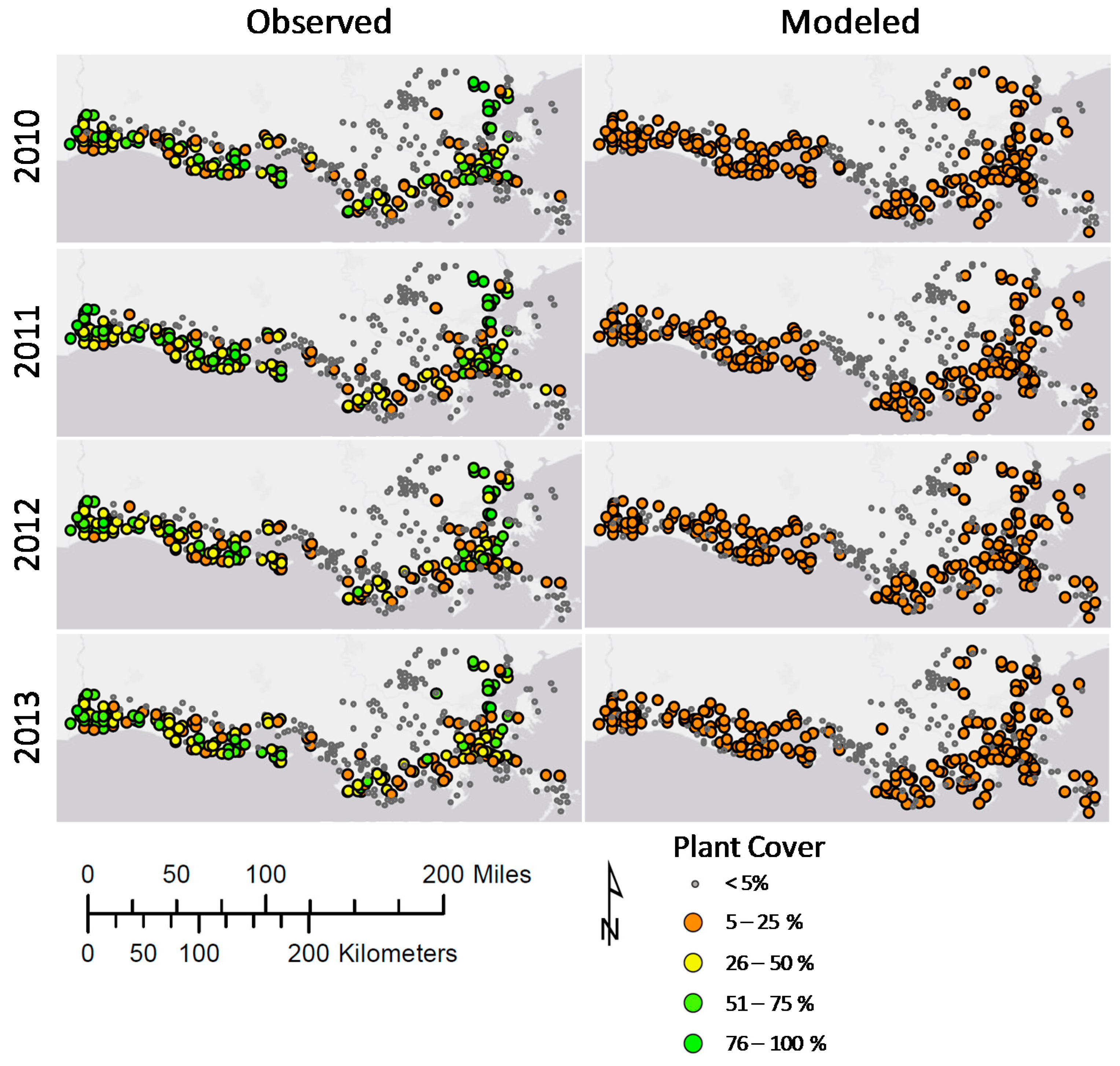
3.1. Model Calibration

For most of the species, the model calibration produced the >80% agreement between the model projections and the observed species distributions (

Table 4. Observed (CRMS) and predicted (LAVegMod.v2) presence/absence of each species in the model for the last year of the calibration period shown as the percentage of 262 stations that represent each category.

Marsh Type	Species	Predicted:	Absent	Present	Absent	Present	Agreement
		Observed:	Absent	Present	Present	Absent
Fresh
	Sagittaria latifolia		98.21	0	1.79	0	98.21
	Cladium jamaiscence		97.62	0	2.38	0	97.62
	Morella cerifera		97.32	0	2.68	0	97.32
	Schoenoplectus californicus		96.43	0	3.57	0	96.43
	Zizaniopsis milliacea		96.13	0	3.87	0	96.13
	Eleocharis baldwinii		95.54	0.30	0	4.17	95.84
	Hydrocotyle umbellatum		94.94	0	5.06	0	94.94
	Panicum hemitomon		92.56	0.30	7.14	0	92.86
	Typha domingensis		78.57	2.68	13.1	5.65	81.25
Intermediate
	Baccharis halimifolia		91.37	0	2.98	5.65	91.37
	Iva frutescens		91.07	0	3.87	5.06	91.07
	Phragmites australis		87.80	0.89	11.01	0.3	88.69
	Sagittaria lancifolia		78.56	3.27	17.86	0.6	81.83
Brackish
	Paspalum vaginatum		89.58	0.60	5.95	3.87	90.18
	Spartina patens		28.87	37.8	17.86	15.48	66.67
Saline
	Avicennia germinans		99.70	0	0.30	0	99.7
	Juncus roemerianus		87.20	0.89	11.31	0.60	88.09
	Spartina alterniflora		70.24	8.33	20.54	0.89	78.57
	Distichlis spicata		64.58	7.14	20.54	7.40	71.72

). Chi-square analysis showed that the modeled distribution of each species was not statistically different from the observed distribution. Sagittaria lancifolia is typical of the agreement between the model and observed distributions for successfully calibrated species (Figure 2). However, the 80% goal was not met for three species: Spartina patens, Distichlis spicata and Spartina alterniflora. Spartina patens showed the lowest level of agreement. Even though the overall percentage of stations occupied in the model and the observed were similar (53% modeled vs. 56% observed), the model predicted presence at 15% of the stations where it was not observed, and the model predicted absence at 18% of the stations where it was observed (Table 4). Spatial distribution shows that the model captures the overall spatial distribution reasonably well (Figure 3), but overestimates the presence of S. patens in what are currently saline marshes as well as intermediate marshes. Some of this is an artifact of the cover of this species being over estimated in the initial 2010 condition.

For D. spicata, the initial condition had significantly lower cover than was observed at the CRMS stations. The model did project increases in D. spicata, but it never reached the observed values and only 69% of the stations were classified correctly at the end of the final calibration run (Table 4). For S. alterniflora, the model shows a decline in cover at the CRMS stations, while the observed cover is relatively stable. Overall, the fit between the model and observations for S. alterniflora was 79%. When examining the spatial distribution of S. alterniflora (Figure 4), it becomes apparent that the model captures the distribution of the area where this species is most prevalent (>25% cover observed).

3.2. Modeled Projects

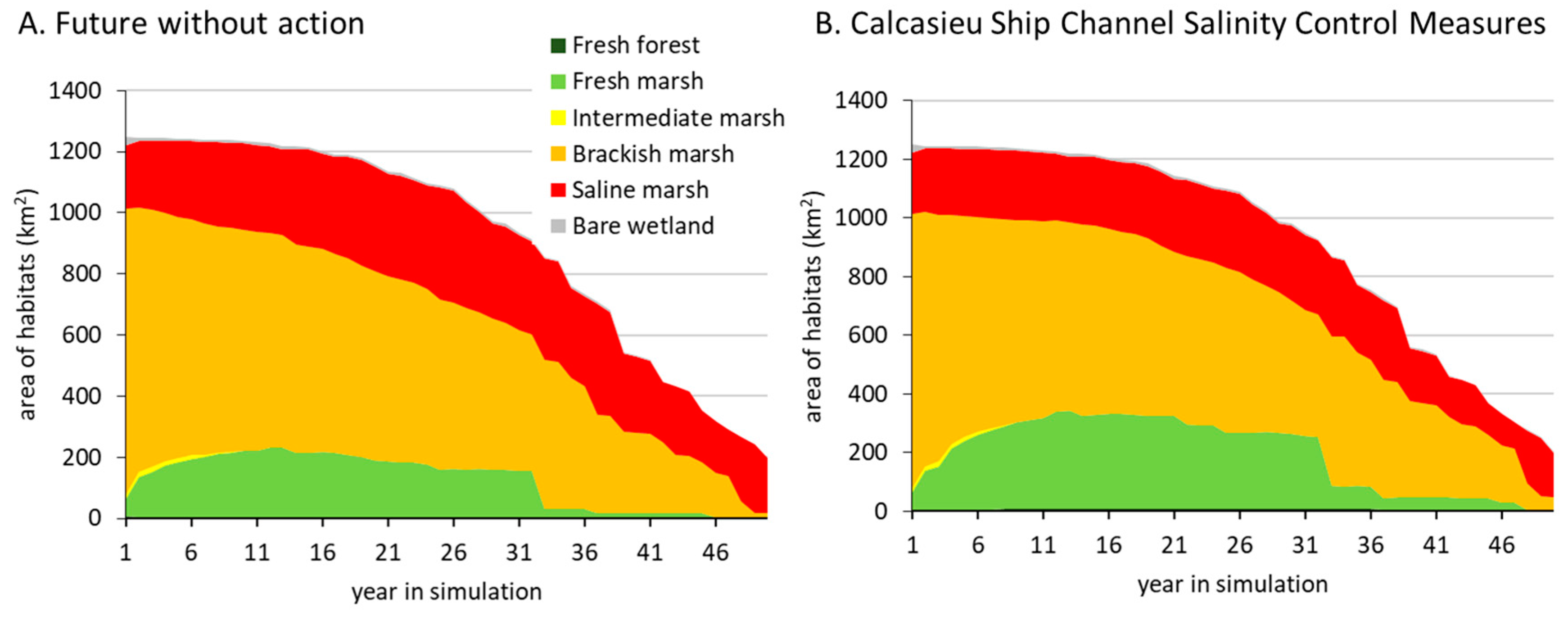
3.2.1. Calcasieu Ship Channel Salinity Control Structures

The Calcasieu Ship Channel Salinity Control Structures, part of the completed 2017 LCMP, reduced salinity in the Calcasieu/Sabine basin. However, these changes in salinity have no effect on land change in the region by year 10 (Figure 5). The salinity changes do affect the vegetation, and there is 67 km² yr⁻¹ more fresh marsh and 3 km² yr⁻¹ more forested wetland in the Calcasieu/Sabine basin with the project than in FWOA, while brackish (−40 km² yr⁻¹) and saline marsh (−30 km² yr⁻¹) both decline by year 10 (Figure 5). At year 20, there is a positive effect of the project on land change in the Calcasieu/Sabine basin, which is due to wetland areas sustained in the inland part of the basin. The project also induces some land loss (conversion of wetland to open water), where fresh marsh occurs among chenier ridges (closer to the coast) due to the project. This fresh marsh is more likely to convert to open water due to salinity intrusion during tropical storms [31]. In FWOA, this area is brackish and less sensitive to salinity increases. At year 20, the project induces land loss outside the Calcasieu/Sabine basin, which is primarily due to a small increase (<2 cm) in the mean annual water level. Therefore, the overall effect of the project on land along the entire coast is negative at this point in the simulation. By year 30, the project has positive effects on land change in both the Calcasieu/Sabine basin and the entire coast. Most of the land loss due to the project occurs in year 24 of the simulation. A large swath of marsh was maintained as fresh marsh with the project through year 23 (Figure 5). In year 24, increased sea level rise combined with land loss in the region allows for more overland flow and thus more saline water to penetrate deeper into the coast, and these fresh marsh areas are lost. In FWOA, the marsh in this region is already brackish, and therefore, less susceptible to the salinity increases associated with the increased overland flow. Drastic land loss occurs throughout the Calcasieu/Sabine basin by years 40 and 50 (Figure 5). The presence of the Calcasieu Ship Channel Salinity Control Measures project allows some wetland areas to be sustained longer than in the FWOA, which results in the land gain associated with the project in years 40 and 50. However, by year 50, most of the wetlands in the area have converted to open water either with or without the project (Figure 5).

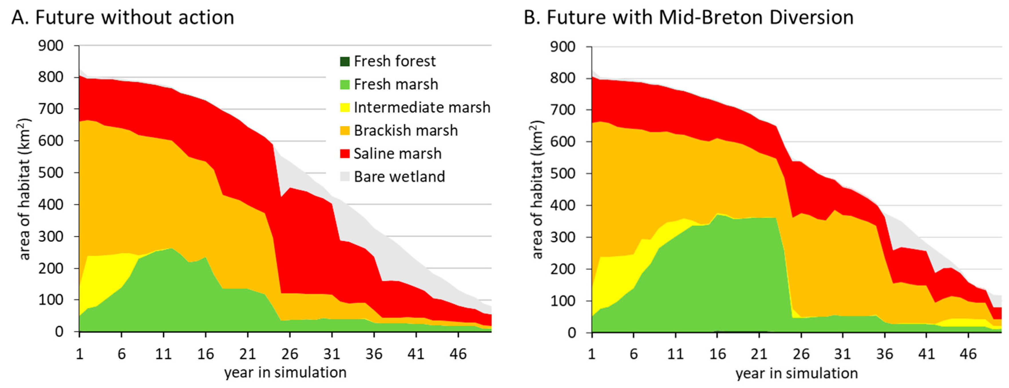
3.2.2. Mid-Breton Sound Diversion

With the Mid-Breton Sound Diversion in place (Year 7), land loss relative to the FWOA occurs between years 11–15 and land gain occurs between years 16–20, with an overall small gain of 2.4 km² in the Breton Sound basin by year 20. In the first 20 years after the diversion is implemented, the simulation shows increases in fresh and intermediate marsh habitats (Figure 6). It is interesting to note that the overall land gain is smaller when considering the entire coast. This is primarily due to accelerated land loss in the Mississippi River Delta (mouth of the Mississippi River), due to less water (and thus sediment) being discharged into the delta as it is removed from the Mississippi River by the Mid-Breton Sound Diversion. The wetland areas at year 30 are somewhat fresher with the diversion than without the diversion (+12.6 km² fresh marsh; +0.7 km² intermediate marsh; +253 km² brackish marsh; and, −204 km² saline marsh) (Figure 6). However, both in the FWOA and with the diversion a major change occurs in this ecoregion in year 24 (Figure 6). This change is due to a combination of land loss and an increased sea level that allows for more overland flow (and thus saline water to move further inland). In the FWOA, this changes most of the Breton Sound basin from brackish to saline marsh, while with the diversion operation results in a change from fresh marsh to brackish marsh (Figure 6). Bare ground that appears under both scenarios is primarily a result of conditions becoming so extreme that they fall outside of the current range of species in the model. It is likely that other species accustomed to higher saline conditions would establish in these places, but these are currently not included in LaVegMod 2.0 or are too distant for the model’s dispersal mechanism to allow colonization.

As relative sea level rises, land loss accelerates rapidly in the Breton Sound basin in the FWOA, but the presence of the diversion is able to prevent some of this loss (Figure 6). In year 40, similar to the previous decade, land loss is accelerated in the central basin due to increased water levels, and only small land gains occur in the immediate outfall area of the diversion. By year 50, fewer areas are sustained and a drop in the overall land gain from the diversion occurs (Figure 6). At the end of 50 years, the diversion sustains existing land and creates new land with sediment input near the diversion, but land loss in this ecoregion continues even with the diversion in place. However, overall there is more land (+48 km²) at the end of 50 years with the project than without it.

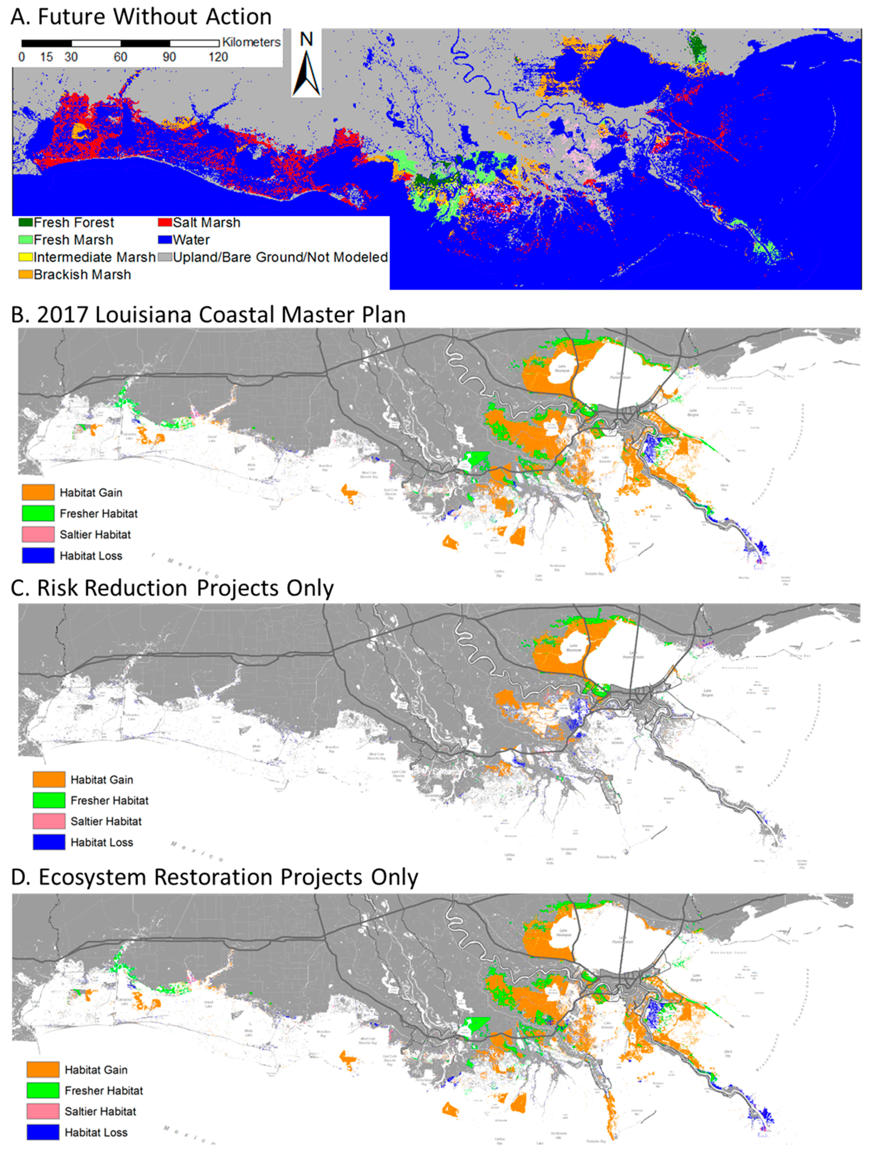
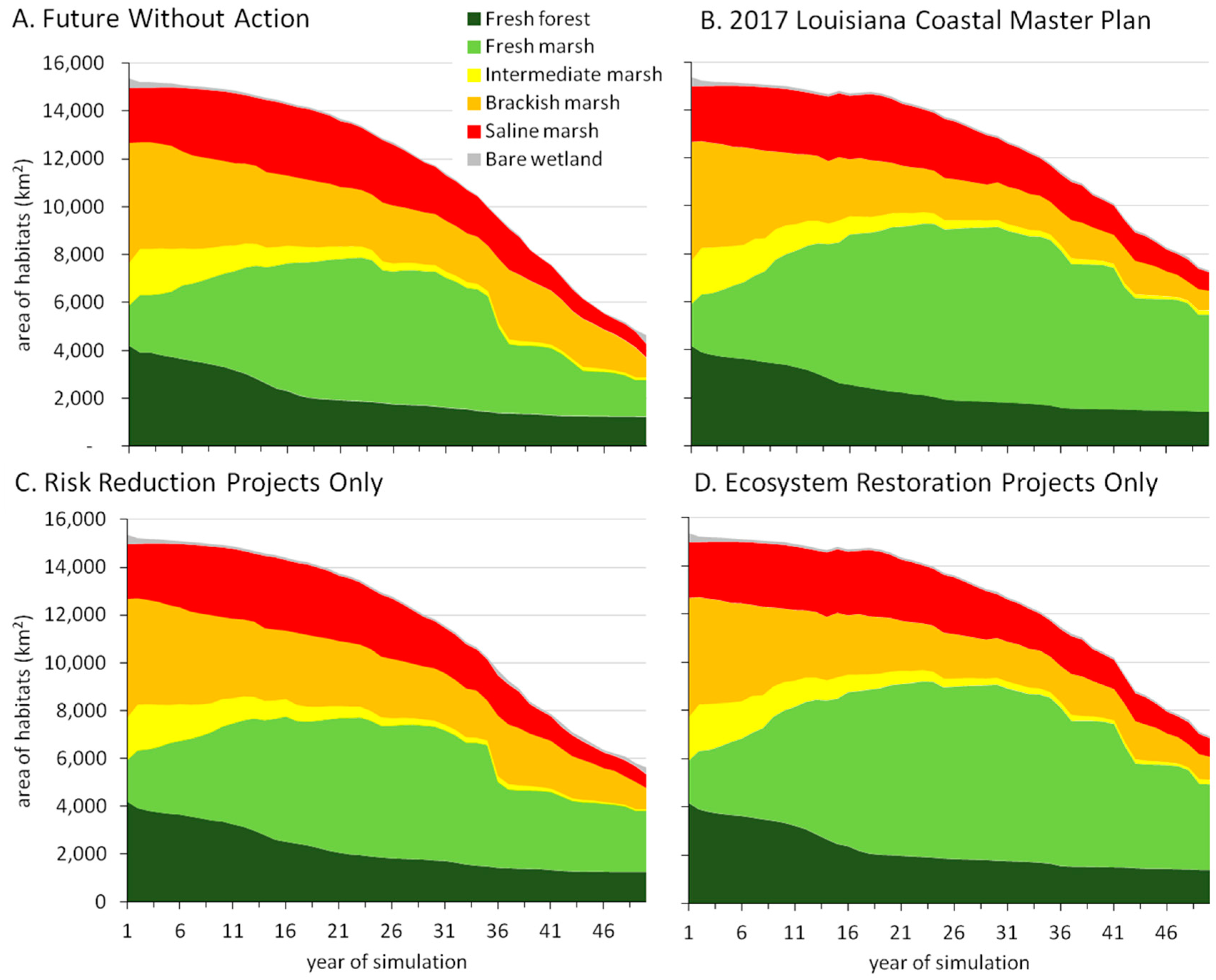
3.2.3. Louisiana Coastal Master Plan

The complete LCMP increases forested wetland (167 km² yr⁻¹), fresh marsh (1540 km² yr⁻¹), and intermediate marsh (17 km² yr⁻¹) relative to the FWOA (Figure 7, Panel B vs. A). However, some of these gains come from losses in brackish (−532 km² yr⁻¹) and saline marsh (−69 km² yr⁻¹). The largest gains occur in the areas affected by sediment diversions in the deltaic plain of the Mississippi river (Figure 8, Panel B). Surprisingly, the risk reduction projects contribute to gains in forested wetland (58 km² yr⁻¹) and fresh marsh (160 km² yr⁻¹) (Figure 8, Panel C). This is due to some of the risk reduction projects limiting tidal exchange to the upper estuary, which slows salinity intrusion. However, the risk reduction projects contribute to land loss in the intermediate (−5 km² yr⁻¹), brackish (−46 km² yr⁻¹) and saline marshes (−6 km² yr⁻¹) relative to the FWOA. This is due to a small increase in water level and salinity coastward of the risk reduction features because they impede fresh water drainage as well as tidal exchange. However, the risk reduction projects have a net positive effect of 184 km² yr⁻¹ relative to the FWOA. The ecosystem restoration projects by themselves have therefore a slightly smaller effect than the complete LCMP. The restoration projects by themselves gain forested wetland (97 km² yr⁻¹), fresh marsh (1515 km² yr⁻¹), and intermediate marsh (11 km² yr⁻¹) and reduce brackish marsh (−452 km² yr⁻¹) and saline marsh (−85 km² yr⁻¹) relative to the FWOA.

4. Discussion

It is important to note that the results shown in this paper represent a “worst case” future scenario for apparent sea-level rise. This scenario was chosen for the evaluation of projects for the incorporation into the 2017 Louisiana Master Plan by the Louisiana Coastal Protection and Restoration Authority, because it leads to selection of projects that are robust in the face of an uncertain future. It is therefore likely that the future predictions shown here (Figure 7, Panel A) exaggerate the loss of coastal wetlands in the next 50 years. However, the realignment of the Louisiana coastline shown here is similar to the map made by Blum and Roberts based only on apparent sea-level rise for 2100 [10].

The predicted landscape at year 50 (Figure 8, Panel A) shows that the marshes are maintained and even grow in those areas affected by water from the Atchafalaya River in the central part of the Louisiana coast. It has been shown that natural processes associated with the synergistic relationship between floods and cold front passages can effectively distribute suspended sediments to maintain and rebuild wetlands outside the sand-rich delta of the Atchafalaya River [32]. Although only 20% of the ecosystem restoration budget in the 2017 LCMP is used for sediment diversion (Table 3), the land gained over the FWOA by ecosystem restoration (Figure 8, Panel D) is largely due to the sediment diversions. However, the use of this restoration technique is limited to areas adjacent to the major rivers and the water and sediment carried by these rivers. In addition, some flow has to remain in the river to allow for navigation

Seventy-one percent of the 2017 LCMP restoration budget is allocated to marsh creation with dredged sediments (Table 3). This ecosystem restoration technique is extremely popular with coastal residents. These projects create land immediately and wetland vegetation establishes rapidly (3–5 years), if land is created at the correct intertidal elevation. However, it has been shown that some of the ecosystem functions of a created marsh take a decade or more or may never reach levels seen in natural marshes [33,34,35,36]. The model results in Figure 8, Panel D also show that some of the created marshes become islands, as surrounding wetlands are lost to apparent sea-level rise. Future versions of the LCMP may need to shift the location of these projects farther inland.

The model presented here was calibrated based on observations from the Louisiana coast and is most applicable to the northern Gulf of Mexico coast. But the model framework could be adapted to other coastal regions of the world.

References

1. Britsch, L.D.; Dunbar, J.B. Land loss rates: Louisiana coastal plain. J. Coast. Res. 1993, 9, 324–338. [Google Scholar]
2. Barras, J.; Beville, S.; Britsch, D.; Hartley, S.; Hawes, S.; Johnston, J.; Kemp, P.; Kinler, Q.; Martucci, A.; Porthouse, J.; et al. Historical and Projected Coastal Louisiana Land Changes: 1978–2050; United States Geological Survey: Reston, VA, USA, 2003; 39p. [Google Scholar]
3. Costanza, R.; Mitsch, W.J.; Day, J.W. A new vision for New Orleans and the Mississippi delta: Applying ecological economics and ecological engineering. Front. Ecol. Environ. 2006, 4, 465–472. [Google Scholar] [CrossRef]
4. Smith, L.M.; Pederson, R.L.; Kaminski, R.M. Habitat Management for Migrating and Wintering Waterfowl of North America; Texas Tech University Press: Lubbock, TX, USA, 1989; ISBN 13 9780896722040. [Google Scholar]
5. Martin, T.E.; Finch, D.M. Ecology and Management of Neotropical Migratory Birds; Oxford University Press: Oxford, UK, 1995; 512p, ISBN 9780195084528. [Google Scholar]
6. Craig, N.J.; Turner, R.E.; Day, J.W. Land loss in coastal Louisiana (USA). Environ. Manag. 1979, 3, 133–144. [Google Scholar] [CrossRef]
7. Scaife, W.W.; Turner, R.E.; Costanza, R. Coastal Louisiana recent land loss and canal impacts. Environ. Manag. 1983, 7, 433–442. [Google Scholar] [CrossRef]
8. Boesch, D.F.; Josselyn, M.N.; Mehta, A.J.; Morris, J.T.; Nuttle, W.K.; Simenstad, C.A.; Swift, D.J. Scientific assessment of coastal wetland loss, restoration and management in Louisiana. J. Coast. Res. 1994, Special Issue 20, 1–103. [Google Scholar]
9. Penland, S.; Ramsey, K.E. Relative sea-level rise in Louisiana and the Gulf of Mexico: 1908–1988. J. Coast. Res. 1990, 6, 323–342. [Google Scholar]
10. Blum, M.D.; Roberts, H.H. Drowning of the Mississippi Delta due to insufficient sediment supply and global sea-level rise. Nat. Geosci. 2009, 2, 488–491. [Google Scholar] [CrossRef]
11. Stone, G.W.; Grymes, J.M., III; Dingler, J.R.; Pepper, D.A. Overview and significance of hurricanes on the Louisiana coast, USA. J. Coast. Res. 1997, 13, 656–669. [Google Scholar]
12. Sifneos, J.C.; Cake, E.W.; Kentula, M.E. Effects of Section 404 permitting on freshwater wetlands in Louisiana, Alabama, and Mississippi. Wetlands 1992, 12, 28–36. [Google Scholar] [CrossRef]
13. Steyer, G.D.; Llewellyn, D.W. Coastal Wetlands Planning, Protection, and Restoration Act: A programmatic application of adaptive management. Ecol. Eng. 2000, 15, 385–395. [Google Scholar] [CrossRef]
14. Reed, D.J.; Wilson, L. Coast 2050: A new approach to restoration of Louisiana coastal wetlands. Phys. Geogr. 2004, 25, 4–21. [Google Scholar] [CrossRef]
15. Twilley, R.R.; Couvillion, B.R.; Hossain, I.; Kaiser, C.; Owens, A.B.; Steyer, G.D.; Visser, J.M. Coastal Louisiana Ecosystem Assessment and Restoration Program: The role of ecosystem forecasting in evaluating restoration planning in the Mississippi River Deltaic Plain. Am. Fish. Soc. Symp. 2008, 64, 29–46. [Google Scholar]
16. Visser, J.M.; Duke-Sylvester, S.M.; Carter, J.; Broussard, W.P. A Computer model to forecast wetland vegetation changes resulting from restoration and protection in coastal Louisiana. J. Coast. Res. 2013. [Google Scholar] [CrossRef]
17. Peyronnin, N.; Green, M.; Richards, C.P.; Owens, A.; Reed, D.; Chamberlain, J.; Groves, D.G.; Rhinehart, W.K.; Belhadjali, K. Louisiana’s 2012 coastal master plan: Overview of a science-based and publicly informed decision-making process. J. Coast. Res. 2013. [Google Scholar] [CrossRef]
18. Coastal Protection and Restoration Authority of Louisiana. Louisiana’s Comprehensive Master Plan for a Sustainable Coast; Coastal Protection and Restoration Authority: Baton Rouge, LA, USA, 2017; 184p. Available online: http://coastal.la.gov/our-plan/2017-coastal-master-plan (accessed on 20 July 2017).
19. Alymov, V.; Cobell, Z.; Couvillion, C.; de Mutsert, K.; Dong, Z.; Duke-Sylvester, S.; Fischbach, J.; Hanegan, K.; Lewis, K.; Lindquist, D.; et al. Appendix C: Modeling Chapter 4—Model Outcomes and Interpretations. In Louisiana’s Comprehensive Master Plan for a Sustainable Coast; Final Version; Coastal Protection and Restoration Authority: Baton Rouge, LA, USA, 2017; 448p. Available online: http://coastal.la.gov/our-plan/2017-coastal-master-plan (accessed on 20 July 2017).
20. Meselhe, E.; McCorquodale, J.A.; Shelden, J.; Dortch, M.; Brown, T.S.; Elkan, P.; Rodrigue, M.D.; Schindler, J.K.; Wang, Z. Ecohydrology component of Louisiana’s 2012 Coastal Master Plan: Mass-balance compartment model. J. Coast. Res. 2013. [Google Scholar] [CrossRef]
21. Couvillion, B.R.; Steyer, G.D.; Wang, H.; Beck, H.J.; Rybczyk, J.M. Forecasting the effects of coastal protection and restoration projects on wetland morphology in coastal Louisiana under multiple environmental uncertainty scenarios. J. Coast. Res. 2013. [CrossRef]
22. Couvillion, B. 2017 Coastal Master Plan Modeling: Attachment C3–27: Landscape Data; Final Version; Louisiana Coastal Protection and Restoration Authority: Baton Rouge, LA, USA, 2017; 84p. Available online: http://coastal.la.gov/wp-content/uploads/2017/04/Attachment-C3–27_FINAL_03.10.2017.pdf (accessed on 25 July 2017).
23. Sasser, C.E.; Visser, J.M.; Mouton, E.; Linscombe, J.; Hartley, S.B. Vegetation Types in Coastal Louisiana in 2013: U.S. Geological Survey Scientific Investigations Map 3290, 1 Sheet, Scale 1:550,000. 2014. Available online: https://pubs.usgs.gov/sim/3290/pdf/sim3290.pdf (accessed on 25 July 2017).
24. Folse, T.M.; West, J.L.; Hymel, M.K.; Troutman, J.P.; Sharp, L.A.; Weifenbach, D.; McGinnis, T.; Rodrigue, L.B.; Boshart, W.M.; Richardi, D.C.; et al. A Standard Operating Procedures Manual for the Coast-Wide Reference Monitoring System—Wetlands: Methods for Site Establishment, Data Collection, and Quality Assurance/Quality Control; Louisiana Coastal Protection and Restoration Authority: Baton Rouge, LA, USA, 2008; 207p. Available online: https://www.lacoast.gov/reports/project/CRMS%20SOP%202012.pdf (accessed on 19 July 2017).
25. Snedden, G.A.; Steyer, G.D. Predictive occurrence models for coastal wetland plant communities: Delineating hydrologic response surfaces with multinomial logistic regression. Estuar. Coast. Shelf Sci. 2013, 118, 11–23. [Google Scholar] [CrossRef]
26. Baldwin, A.H.; Mendelssohn, I.A. Effects of salinity and water level on coastal marshes: An experimental test of disturbance as a catalyst for vegetation change. Aquat. Bot. 1998, 61, 255–268. [Google Scholar] [CrossRef]
27. Ross, M.S.; Meeder, J.F.; Sah, J.P.; Ruiz, P.L.; Telesnicki, G.J. The southeast saline Everglades revisited: 50 years of coastal vegetation change. J. Veg. Sci. 2000, 11, 101–112. [Google Scholar] [CrossRef]
28. Hayden, B.P.; Santos, M.C.; Shao, G.; Kochel, R.C. Geomorphological controls on coastal vegetation at the Virginia Coast Reserve. Geomorphology 1995, 13, 283–300. [Google Scholar] [CrossRef]
29. Meselhe, E.; White, E.D.; Reed, D.J. 2017 Coastal Master Plan: Appendix C: Modeling Chapter 2—Future Scenarios. In Louisiana’s Comprehensive Master Plan for a Sustainable Coast; Final Version; Coastal Protection and Restoration Authority: Baton Rouge, LA, USA, 2017; 32p. Available online: http://coastal.la.gov/wp-content/uploads/2017/04/Appendix-C_chapter2_FINAL_3.16.2017.pdf (accessed on 27 July 2017).
30. Kent, M.; Coker, P. Vegetation Description and Analysis: A Practical Approach; Bell Haven Press: London, UK, 1992; 384p, ISBN 13 978-0471948100. [Google Scholar]
31. Couvillion, B.R.; Beck, H. Marsh collapse thresholds for coastal Louisiana estimated using elevation and vegetation index data. J. Coast. Res. 2013. [Google Scholar] [CrossRef]
32. Roberts, H.H.; DeLaune, R.D.; White, J.R.; Li, C.; Sasser, C.E.; Braud, D.; Weeks, E.; Khalil, S. Floods and cold front passages: Impacts on coastal marshes in a river diversion setting (Wax Lake Delta area, Louisiana). J. Coast. Res. 2015, 31, 1057–1068. [Google Scholar] [CrossRef]
33. Zedler, J.B.; Callaway, J.C. Tracking wetland restoration: Do mitigation sites follow desired trajectories? Restor. Ecol. 1999, 7, 69–73. [Google Scholar] [CrossRef]
34. Craft, C.; Broome, S.; Campbell, C. Fifteen years of vegetation and soil development after brackish-water marsh creation. Restor. Ecol. 2002, 10, 248–258. [Google Scholar] [CrossRef]
35. Craft, C.; Megonigal, P.; Broome, S.; Stevenson, J.; Freese, R.; Cornell, J.; Zheng, L.; Sacco, J. The pace of ecosystem development of constructed Spartina alterniflora marshes. Ecol. Appl. 2003, 13, 1417–1432. [Google Scholar] [CrossRef]
36. Moreno-Mateos, D.; Power, M.E.; Comín, F.A.; Yockteng, R. Structural and functional loss in restored wetland ecosystems. PLoS Biol. 2012, 10, e1001247. [Google Scholar] [CrossRef] [PubMed] [Green Version]
Figure 1. Distribution of Coastwide Reference Monitoring System (CRMS) stations across the Louisiana coast. Stations are color coded by the habitat type observed at the station in 2015. Size of the dots is not to scale to the 200 × 200 m study area at each station. Hydrologic basins are outlined in white and shows the general extend of the ICM model domain (without boundary areas).
Sustainability 09 01625 g001
Figure 2. Spatial distribution of Sagittaria lancifolia as observed at CRMS sites and as predicted for those same sites by the calibrated model. Each point is the location of a single CRMS station. Large colored dots represented stations where S. lancifolia was either observed (A) or predicted by the model (B) at or above 5% cover. Small grey dots are stations where S. lancifolia was either not observed (A) or not predicted to occur by the model (B). Terrestrial areas are shown in light grey while the Gulf of Mexico is shown in darker grey.
Sustainability 09 01625 g002
Figure 3. Spatial distribution of Spartina patens as observed at CRMS sites and as predicted for those same sites by the calibrated model.
Sustainability 09 01625 g003
Figure 4. Spatial distribution of Spartina alterniflora as observed at CRMS sites and as predicted for those same sites by the calibrated model. Each point is the location of a single CRMS station.
Sustainability 09 01625 g004
Figure 5. Change in wetland habitats in the Calcasieu/Sabine basin. Panel A shows the future without action and Panel B shows the future with the Calcasieu Ship Channel Salinity Control Measures.
Sustainability 09 01625 g005
Figure 6. Change in wetland habitats in the Breton Sound basin. Panel A shows the future without action and Panel B shows the future with the Mid Breton Sound Diversion.
Sustainability 09 01625 g006
Figure 7. Coastwide wetland habitat change simulated for (A) the future without action (FWOA), (B) the Complete Master Plan, (C) simulations that only include risk reduction projects and (D) a simulation that included only the ecosystem restoration projects. For clarity only wetland area is shown, the upland area (1789 km2) is assumed to remain the same by the Integrated Compartment Model (ICM), and decreases in wetland reflect conversion to open water. At the start of the simulation open water covers 20,891 km2.
Sustainability 09 01625 g007
Figure 8. Coastwide habitat distribution at year 50 for (A) the FWOA, and habitat change forecasted at year 50 for (B) the Complete Master Plan, (C) simulations that only include risk reduction projects, and (D) a simulation that included only the ecosystem restoration projects.
Sustainability 09 01625 g008