The Supply Chain Design for Perishable Food with Stochastic Demand

1
School of Economics and Management, Changshu Institute of Technology, Changshu 215500, China
2
Jiangsu Key Laboratory of Modern Logistics, School of Marketing and Logistics Management, Nanjing University of Finance and Economics, Nanjing 210023, China
3
Business School, Nanjing University, Nanjing 210093, China
4
Stanley Ho Big Data Decision Analytics Research Centre, the Chinese University of Hong Kong, Shatin, New Territories, Hong Kong 999077, China
*
Author to whom correspondence should be addressed.
Sustainability 2017, 9(7), 1195; https://doi.org/10.3390/su9071195
Submission received: 25 May 2017
/
Revised: 23 June 2017
/
Accepted: 30 June 2017
/
Published: 11 July 2017
(This article belongs to the Section Economic and Business Aspects of Sustainability)
Abstract
:It has been a challenging task to manage perishable food supply chains because of the perishable product’s short lifetime, the possible spoilage of the product due to its deterioration nature, and the retail demand uncertainty. All of these factors can lead to a significant amount of shortage of food items and a substantial retail loss. The recent development of tracing and tracking technologies, which facilitate effective monitoring of the inventory level and product quality continuously, can greatly improve the performance of food supply chain and reduce spoilage waste. Motivated by this recent technological advancement, our research aims to investigate the joint decision of pricing strategy, shelf space allocation, and replenishment policy in a single-item food supply chain setting, where our goal is to maximize the retailer’s total expected profit subject to stochastic retail demand. We prove the existence of optimality for the design of the perishable food supply chain. We then extend the single-item supply chain problem to a multi-item setting and propose an easy-to-implement searching algorithm to produce the optimal allocation of shelf space among these items for practical implementation. Finally, we provide numerical examples to demonstrate the effectiveness of our solution.
1. Introduction
With the fast pace of modern life, it has become more common to buy perishable food items in marts or retail groceries. Perishable food becomes an important factor that customers may consider when choosing one retail store among others [1]. The increasing demand for perishable food leads to a higher profit; meanwhile, larger quantities and a wider variety of food items impose further challenges on the management of the supply chain [2,3,4]. The deterioration and demand uncertainty of perishable food result in a large portion of the items being unsalable and frequent shortages of products in retail stores. The attrition rate of perishable food can reach 15% in retail stores and hence causes costs of billions of dollars, for example, in European groceries [5,6]. The mass spoilage and difficulty in management impel retailers to set a higher retail price, which retains the consumption and results in frequent shortages. Besides the economic aspect, the perishability of these food items also distinguishes their supply chains from the traditional ones because this feature is crucial to the sustainability of the system. Waste resulting from unsalable perishable food items and their implications for energy usage cause significant environmental impacts. A more sustainable perishable food supply chain not only requires efforts of every individual party involved, but also an efficient coordination among them. All of the above characteristics of perishable food items motivate us to study the design of this supply chain system.
The development of modern identification and sensory technologies, such as temperature and humidity sensors and RFID technology, could monitor the ambient environment and track the consumption continuously. These technologies enable managers of the companies to establish an agile food supply chain and hence improve the management of perishable food products. Since the decaying quality of perishable food leads to a demand slowdown, food retailers tend to implement promotion strategies to improve the efficiency of the food supply chain. Since perishable food demands are generally price-sensitive, provision of discount on the items may increase the consumption rate when food quality decay. On the other hand, a larger shelf space may attract more customers. Therefore, a better allocation of shelf space may improve its utilization and result in a higher profit. In this research, we aim to determine the optimal pricing and discount strategies, shelf space allocation decisions, and replenishment policy that jointly maximize the food retailer’s expected profit with the consideration of stochastic retail demand.
With the modern identification and tracking technologies, advanced logistics management information systems could be developed for the perishable product management [7,8,9]. There has been extensive work on improving the management of perishable products, where three main approaches have been adopted to model the characteristics of the perishability of food items. First, the perishable product is assumed to have a fixed or random lifetime. For example, Petruzzi and Dada [10] provided a review on incorporating pricing into the newsvendor model with stochastic demand and a fixed lifetime. Goyal and Giri [11] reviewed the inventory models with deteriorating items, in which the model for perishable products with a random lifetime is introduced. Second, there have been studies that assumed that a proportion of perishable products become unsalable after transshipment, while the rest retains the full value. For instance, Mandal and Phaujdar [12] developed an inventory model for perishable items, assuming that the deterioration rate could be constant or time-dependent and that the demand rate is a linear function of the instantaneous stock level. Wee [13] proposed a joint pricing and replenishment policy for the perishable items with a declining demand. Third, some studies assume the value of a perishable product decays over time due to deterioration. Zanoni and Zavanella [14] developed a sustainable food supply chain, taking energy efforts into account, with the assumption that the quality of perishable food decays exponentially. With the same assumption, Rong et al. [15] developed a mixed-integer linear programming model for production and distribution planning. Our research also follows the majority of existing literature and is developed based on the third assumption. Since the demands of most of the perishable products are price-sensitive and decrease over time, the pricing strategy has a significant influence on the effectiveness of a sales promotion, especially when the promotion date is close to the expiration of the product. Wang and Li [1] proposed a pricing model with single and multiple markdowns to maximize the retailer’s profit in a perishable food supply chain.
Besides the perishable product’s quality and price, the customer demand is also impacted by the shelf space allocated to the product [16,17,18,19,20]. The rationale is that a larger shelf space has a higher visibility to customers and hence may induce greater sales. Desmet’s and Renaudin’s investigation [16] confirmed that direct shelf space elasticities are non-zero for numerous types of products. Lynch and Curhan [17] assumed a quadratic relationship between the shelf space allocated to a product and its demand rate in supermarkets. Mohsen et al. [18] considered a two-stage inventory setting, where a warehouse and a display shelf are involved in an integrated vendor-buyer inventory model, and where the demand is dependent on the number of items visible to the customers. As there are only a few papers in the literature which incorporated stochastic demand into the perishable food supply chain, our research aims to design an efficient food supply chain by deriving the optimal joint decisions of pricing and discount strategy, shelf space allocation, and replenishment policy.
The remainder of this paper is organized as follows. Section 2 provides our proposed approach to modeling the quality of the perishable items and then develops the fundamental model for representing the perishable food supply chain. In Section 3, we derive the optimal solution for the design of such supply chain. Section 4 presents the optimal solution methodology, and Section 5 provides a numerical study to demonstrate its effectiveness. Section 6 discusses the results and presents future research opportunities.
2. Model Formulation for the Single-Item Food Supply Chain
In this section, we first model the retail demand and then develop the fundamental mathematical model for the whole process regarding the sales of perishable food in a retail store, including product arrival, sales induced by the shelf space allocation decision, and the disposal of the expired goods.
2.1. Quality Deterioration
Quality degradation is a major issue for the perishable food. Tracking and predicting the quality of perishable food was a challenging and costly task prior to the introduction of modern sensing technologies, such as RFID tools and humidity-temperature sensors. Nowadays, with these technologies and quality prediction models, parties in the perishable food industry can make a more accurate prediction about the remaining shelf life or the product quality, which are the retailers’ main concerns and can greatly influence the retail demand.
According to Labuza [21], the quality degradation of perishable food is affected by several factors, such as storage time, temperature, and ambient atmosphere condition. More specifically, the quality degradation can be expressed by the following equation:
where q is the quality of a perishable product, k is the rate of degradation, and n is the chemical order of the reaction. In Equation (1), n could be equal 0 or 1, for the facilitation of two types of different degradation models. When n = 0, the quality decays at a constant rate. When n = 1, the quality decays exponentially. This setting appears to be more realistic and hence has been used widely in research relevant to perishable food items. For this reason, our research assumes n = 1. In Equation (1), k can be expressed as
where k0 is a constant, Ea is the activation energy, which can be estimated from empirical data, R is the gas constant, and T0 is the absolute temperature. According to Equations (1) and (2), the quality of perishable product at time t can be modelled by
where q0 is the initial quality. In most retail groceries, the temperature and atmosphere condition are relatively stable. Therefore, we introduce λ as the deterioration rate to simplify the mathematical expression. Let
Hence, the quality at time t becomes
2.2. Demand Model
In a mart or retail grocery, the consumption rate of perishable food can be influenced by a number of factors, such as customer arrival rate, retail price, food quality, discount rate, shelf space, and location of the shelf. Our research considers that the consumption rate depends on four key factors: market scale, a, selling price, p, product quality at time t, q(t), and shelf space allocated to the product, ng. We assume that the customers can distinguish the food quality by observation and a larger shelf space allocated to the product can induce higher sales due to the enhanced visibility. We model these features by a linear relationship between the retail demand and the factors. This linear model has been adopted in the literature, for example, in Swami and Shah [22]. More specifically, the demand can be characterized by
In Equation (6), b, c, and d are all nonnegative constant parameters, representing price elasticity, demand sensitivity to shelf space and product quality, respectively. ε is a random variable to model the fluctuation of demand, which follows a uniform distribution ε ∈ U[−L, L].
As time goes, the food items decay, their shelf life is about to end and the retail demand rate will go down accordingly. In most situations, the retailer will offer a discount on these products and reallocate them from the original shelves to a discount rack. As a result, the shelf space begins to have no effect on the sales and the discount rack starts to boost the sales. Therefore, the demand function after discount imposed on the items is
where a, b, and d are the same as in D1(t), 1 − θ is the discount rate, and f is the discount rack attraction rate.
Let t0 and T respectively denote the times that the products are on the non-discount shelf and their shelf life. To summarize, the demand function can be expressed as
Thus, the total demand on the non-discount shelf is
The total demand on discount rack is
Let D1 and D2 represent the expected demands on the non-discount shelf and the discount rack, respectively,
Then, the stochastic part of demand is εt0 + ε(T − t0) = εT ∈ [−LT, LT], as ε ∈ U[−L, L].
2.3. Modeling the Food Supply Chain
In the previous sections, we have modeled the quality deterioration process and the retail demand over the whole shelf life. Now we aim to develop the profit function for the retail stores. There are several key factors that influence the retailer’s profit: sales revenue, shelf space cost, purchasing cost, shortage cost, and disposal cost.
The expected sales revenue resulting from the sales of the product generated when they are on the non-discount shelve is
When a shelf space of ng units is allocated to the product, the associated cost is mng2 per unit time, where m is the opportunity cost due to the shelf allocation. Since a shelf space of ng unit is allocated to the product from the beginning to t0, there is an associated cost t0mng2.
The expected sales revenue resulting from the sales of the product generated when they are on the discount rack, from t0 to T, is
Let Q and C0 denote the order quantity and purchasing cost per unit, respectively. The total purchasing cost is C0Q.
Since the demand is stochastic, we also consider the possibility of retail shortage. Let Cs denote the shortage cost per unit. The total expected shortage cost is
Finally, there can be a certain amount of items, which cannot be sold out by the end of shelf life. These remaining items will need to be disposed of, and the disposal process may generate carbon emissions, produce environmental pollution, and incur disposal costs. Let Cd denote the disposal cost per unit. Then, the total expected disposal cost is
To summarize, the total expected profit of the food supply chain is
In Equation (17), we determine p, ng, and Q that maximize the total expected profit.
3. The Optimal Solution for the Single-Item Food Supply Chain
In this section, we prove the existence of an optimal solution that maximizes the total expected profit.
We observe that the total expected profit E(π) is a polynomial function of p, given that Q and ng are constant. Taking the first and second derivatives of E(π) with respect to p, we have
Thus, E(π) is a concave function of p.
Then, taking the first derivative of E(π) with respect to Q and ng,
The necessary condition to maximize E(π) is . The Hessian matrix of E(π) is
In Equation (22),
Therefore,
The total expected profit is concave when p is determined and fixed, and hence the optimal solution can be obtained by solving the set of equations .
We propose a solution methodology as follows (Algorithm 1).
| Algorithm 1: Solution Methodology for Single-Item Food Supply Chain |
|
4. The Multi-Item Food Supply Chain
In this section, we extend the single-item supply chain problem to a multi-item setting. Here, we make further assumptions to simplify the more complicated problem. First, these products cannot substitute the others. In other words, each product’s demand is independent of that of the others. Second, the capacity of shelf space available is limited. Third, all the items are replenished separately, and the ordering cost is ignored since the replenishment cycle of each item is fixed. Fourth, since each item’s replenishment cycle may be different, we maximize the total expected profit in a unit of time instead of the total expected profit per cycle in the single-item model.
Let superscript i denote the index of the items sold in the perishable food shelves and S denote the shelf space capacity. Therefore, the total expected profit per unit of time for the multi-item food supply chain is
In Equation (27), similar to the single-item setting, pi, ngi, Qi, and m are the decision variables. In physical retail stores, the shelf space cost (t0imngi) of each item is usually not included in the retailer’s profit; however, it is still a major concern when the retailer decides whether a product should be sold in the store and how much shelf space should be allocated to the product. Therefore, the total expected profit per unit of time without shelf space cost is
We propose an easy-to-implement searching algorithm to obtain an optimal solution. Equation (27) suggests that an optimal solution for each item would be different once the opportunity cost of shelf space (m) is given because the replenishment cycle (Ti) of each item is constant. We observe that the opportunity cost of shelf space is negatively correlated with each item’s allocated shelf space and profit. Therefore, the lowest m which makes ∑inig ≤ S is the optimal solution.
We propose a solution methodology as follows (Algorithm 2).
| Algorithm 2: Solution Methodology for Multi-Item Food Supply Chain |
|
5. Numerical Experiment
In this section, we conduct numerical experiments and examine the effects of the key parameters on the total expected profit and the optimal solution. First, we evaluate the effects of the discount rate (θ), demand uncertainty (L), and deterioration rate (λ) on the results in the single-item supply chain. Table 1 shows the values of input parameters, some of which were examined in Wang and Li [1].
In the mathematical model presented in Section 2, we assumed that the discount rate 1 − θ is constant; however, this discount rate is also an important decision of the retail store in practice. For this reason, we attempt to approximate the optimal discount rate by conducting a numerical analysis.
The optimal solutions with different θ by Algorithm 1 are collected in Table 2. Table 2 shows that, as discount rate decreases, the shelf space allocated, price, and order quantity all decrease. This phenomenon is because the reduction in discount rate decreases the demand for the product when the items are on the discount rack, and the retailer has to lower the price to induce the sales and the shelf space to reduce shelf space cost. From Figure 1, we can see that the total profit appears to be concave in θ and reaches its maximum around θ = 0.9. In the retail store, the demand uncertainty is one of the most important factors that can affect the profit significantly. Figure 2 shows the expected profit with different levels of demand variance.
Figure 2 shows that the total expected profit is negatively correlated with the demand variance. The price, order quantity, and shelf space allocation remain the same as those obtained previously (θ = 0.85) in Table 2. Hence, it appears that demand fluctuation effects could not be reduced by adjusting the pricing and shelf space allocation strategies. This demonstrates the reason that the perishable food supply chain is difficult to manage. To overcome it, some marts choose to mark down several times to diminish the effect of fluctuation. Therefore, the demand prediction and flexible promotion strategies are particularly important in food supply chain management.
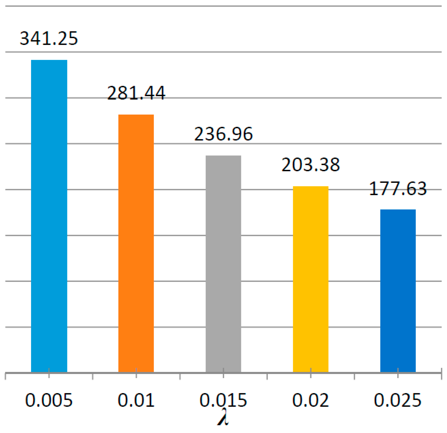
With different kinds of perishable foods, the deterioration rate varies significantly. For example, the quality of canned food decays slowly, while fresh fish and deli may perish in a few hours. Therefore, the deterioration rate can greatly affect the replenishment policy and pricing strategy. Figure 3 and Table 3 show the expected profit and optimal solution with different deterioration rates.
Table 3 shows that as the deterioration rate increases, the retailer prefers to reduce the shelf space, order quantity, and price to respond. In reality, the retailer may also shorten the replenishment cycle to diminish the effect of deterioration. However, both strategies increase the operational cost and hence reduce the expected profit, as shown in Figure 3. As the food with high deterioration rate is mostly sold in the early replenishment cycle, the retailer may often either run out of stock in a short period of time or the rest of products that could not be sold at an early stage remain to the expiration date. For the food retailers, modern tracing and tracking technologies and flexible promotion strategies could be applied to increase the food supply chain efficiency and reduce the spoilage waste.
In the second case, we evaluate the effect of the shelf space capacity. Since the shelf space capacity is one important factor when customers decide the mart or retail store for grocery shopping. In general, large marts, which provide a comfortable shopping environment and a wide variety and lower prices of retail products, are more popular. Table 4 shows the characteristics of the computational experiments for a four-item supply chain.
The results of the multi-item retail chain with different S from Algorithm 2 are collected in Table 5. Table 5 shows the total expected profit per unit of time and each item’s optimal solutions with different shelf space capacities.
From Table 5, we can observe that, as the capacity increases, the total profit increases accordingly. With the same items, the profit still increases exponentially. In reality, the retailer could add new items, which may bring about additional profit. Therefore, large marts could enjoy the shelf space scale of economies, and this superiority creates a hard time for the nearby small groceries to compete. On the other hand, small groceries may have advantages over large marts. For example, less shelf space and a lower variety of products allow small groceries to provide prompt and convenient service. Therefore, increasing the variety of products may not be a suitable option for retailers when a larger shelf space is available.
6. Conclusions
This paper attempts to improve the design of food supply chain in a retail store by comprehensively evaluating the pricing strategy, shelf space allocation, and replenishment policy with the support of modern tracing and tracking technologies. This paper provides a solution framework for achieving great potential of spoilage reduction and profit improvement for food supply chain with stochastic demand. Our results suggest that the discount rate is closely related to other decisions in this supply chain and its optimal value can be derived numerically. As the deterioration and demand variance further complicate the operations, a flexible promotion and replenishment policy should be adopted to reduce these effects. Large marts could enjoy the shelf space scale of economies, and increasing the variety of products and each item’s shelf space could increase the profit when larger shelf space is available. As shown in the experiments, a number of factors can impact the profit significantly. Thus, all of these key factors should be evaluated precisely when the food retail supply is designed.
Our proposed model can be extended in two directions. First, other types of demand distributions, such as Normal distribution and Poisson distribution, can be considered in the model. Second, the coordination policies with suppliers would be worth investigating.
Acknowledgments
The authors are grateful to the editors and anonymous reviewers for providing the valuable comments. The research was supported by the National Natural Science Foundation of China (Grant No. 71501090) and the Jiangsu Philosophical-social Science Program (2016SJB630113).
Author Contributions
Yujie Xiao and Shuai Yang contributed equally to this work. Yujie Xiao conceived and designed the experiments; Shuai Yang performed the experiments; Yujie Xiao and Shuai Yang analyzed the data; Yong-Hong Kuo contributed analysis tools; Yujie Xiao and Shuai Yang wrote the paper.
Conflicts of Interest
The authors declare no conflict of interest. The founding sponsors had no role in the design of the study; in the collection, analyses, or interpretation of data; in the writing of the manuscript; or in the decision to publish the results.
References
- Wang, X.; Li, D. A dynamic product quality evaluation based pricing model for perishable food supply chains. Omega 2012, 40, 906–917. [Google Scholar] [CrossRef]
- Chung, S.H.; Kwon, C. Integrated supply chain management for perishable products: Dynamics and oligopolistic competition perspectives with application to pharmaceuticals. Int. J. Prod. Econ. 2016, 179, 117–129. [Google Scholar] [CrossRef]
- Minner, S.; Transchel, S. Order variability in perishable product supply chains. Eur. J. Oper. Res. 2017, 260, 93–107. [Google Scholar] [CrossRef]
- Xiao, Y.; Yang, S. The retail chain design for perishable food: The case of price strategy and shelf space allocation. Sustainability 2017, 9, 12. [Google Scholar] [CrossRef]
- Ferguson, M.E.; Ketzenberg, M.E. Information Sharing to Improve Retail Product Freshness of Perishables. Prod. Oper. Manag. 2006, 15, 57–73. [Google Scholar]
- Karkkainen, M. Increasing efficiency in the supply chain for short shelf life goods using RFID tagging. Int. J. Retail Distrib. Manag. 2003, 31, 529–536. [Google Scholar] [CrossRef]
- Hertog, M.L.A.T.M.; Uysal, I.; McCarthy, U.; Verlinden, B.M.; Nicolaï, B.M. Shelf life modelling for first-expired-first-out warehouse management. Philos. Trans. R. Soc. A Math. Phys. Eng. Sci. 2014, 372, 1–15. [Google Scholar] [CrossRef] [PubMed]
- Sciortino, R.; Micale, R.; Enea, M.; La Scalia, G. A WebGIS-based System for Real Time Shelf Life Prediction. Comput. Electron. Agric. 2016, 127, 451–459. [Google Scholar] [CrossRef]
- La Scalia, G.; Settanni, L.; Corona, O.; Nasca, A.; Micale, R. An innovative shelf Life model based on smart logistic unit for an efficient management of the perishable food supply chain. J. Food Process Eng. 2015. [Google Scholar] [CrossRef]
- Petruzzi, N.; Dada, M. Pricing and the newsvendor problem: A review with extensions. Oper. Res. 1999, 47, 183–194. [Google Scholar] [CrossRef]
- Goyal, S.K.; Giri, B.C. Recent trends for modeling deteriorating inventory. Eur. J. Oper. Res. 2001, 134, 1–16. [Google Scholar] [CrossRef]
- Mandal, B.N.; Phaujdar, S. An inventory model for deteriorating items and stock-dependent consumption rate. J. Oper. Res. Soc. 1989, 40, 483–488. [Google Scholar] [CrossRef]
- Wee, H.M. Joint pricing and replenishment policy for deteriorating inventory with declining market. Int. J. Prod. Econ. 1995, 40, 163–171. [Google Scholar] [CrossRef]
- Zanoni, S.; Zavanella, L. Chilled or frozen? Decision strategies for sustainable food supply chains. Int. J. Prod. Econ. 2012, 140, 731–736. [Google Scholar] [CrossRef]
- Rong, A.; Akkerman, R.; Crunow, M. An optimization approach for managing fresh food quality throughout the supply chain. Int. J. Prod. Econ. 2011, 131, 421–429. [Google Scholar] [CrossRef]
- Desmet, P.; Renaudin, V. Estimation of product category sales responsiveness to allocated shelf space. Int. J. Res. Mark. 1998, 15, 443–457. [Google Scholar] [CrossRef]
- Lynch, M.; Curhan, R.C. A Comment on Curhan’s “The relationship between shelf space and unit sales in supermarkets”. J. Mark. Res. 1974, 11, 218–220. [Google Scholar] [CrossRef]
- Mohsen, S.S.; Anders, T.; Mohammad, R.A.J. An integrated vendor-buyer model with stock-dependent demand. Transp. Res. E Logist. 2010, 46, 963–974. [Google Scholar]
- Pawlewski, P. DES/ABS Approach to Simulate Warehouse Operations. In Highlights of Practical Applications of Agents, Multi-Agent Systems, and Sustainability—The PAAMS Collection; Springer International Publishing: Salamanca, Spain, 2015; pp. 115–125. [Google Scholar]
- Grzybowska, K.; Awasthi, A.; Hussain, M. Modeling enablers for sustainable logistics collaboration integrating—Canadian and Polish perspectives. In Proceedings of the 2014 Federated Conference on Computer Science and Information Systems, Warsaw, Poland, 7–10 September 2014; pp. 1311–1319. [Google Scholar]
- Labuza, T.P. Shelf-Life Dating of Foods; Food and Nutrition Press: Westport, CT, USA, 1982. [Google Scholar]
- Swami, S.; Shah, J. Channel coordination in green supply chain management. J. Oper. Res. Soc. 2013, 64, 336–351. [Google Scholar] [CrossRef]
Figure 1.
Total expected profit of the retail chain with different θ.
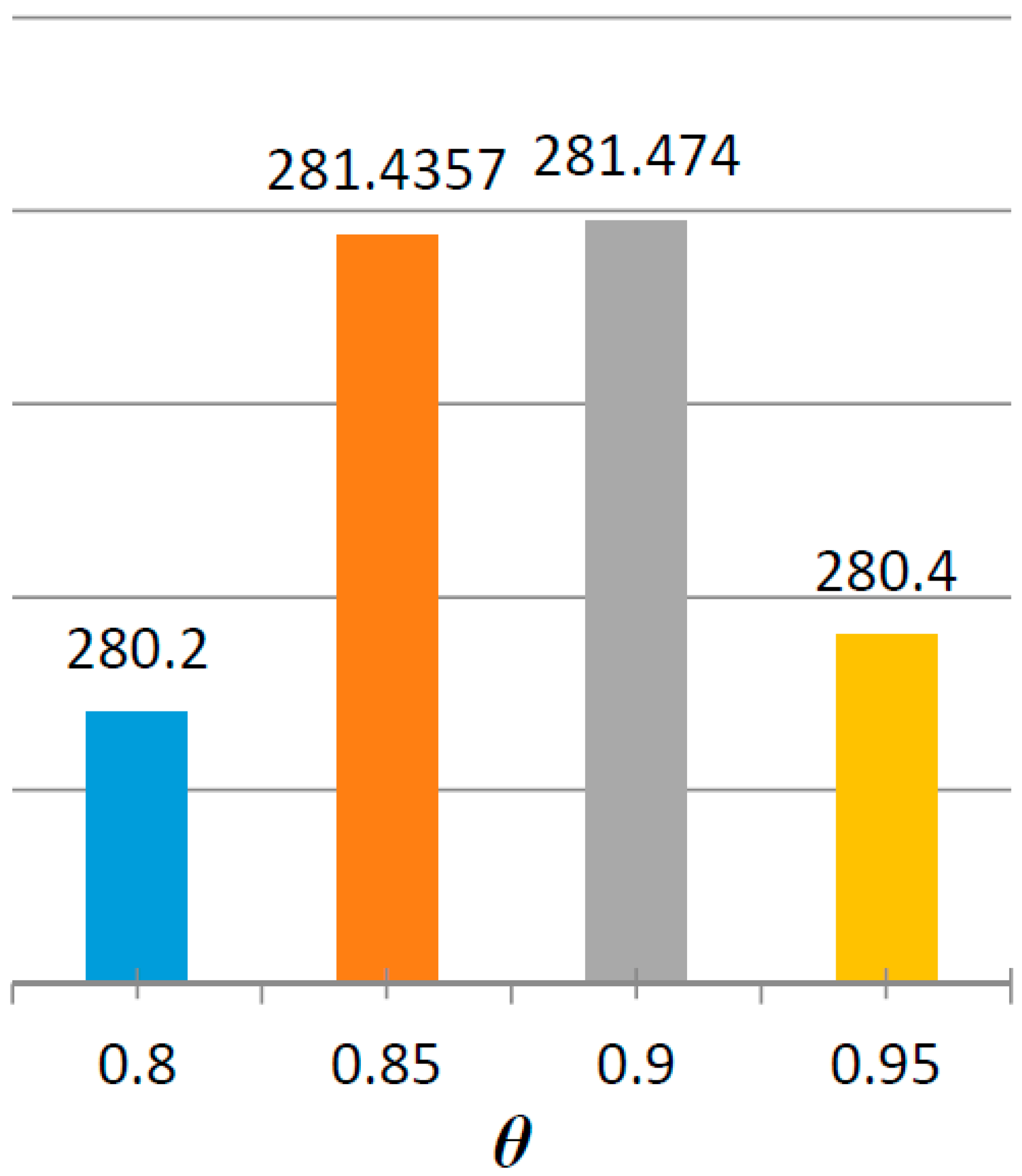
Figure 2.
Total expected profit of the retail chain with different L.
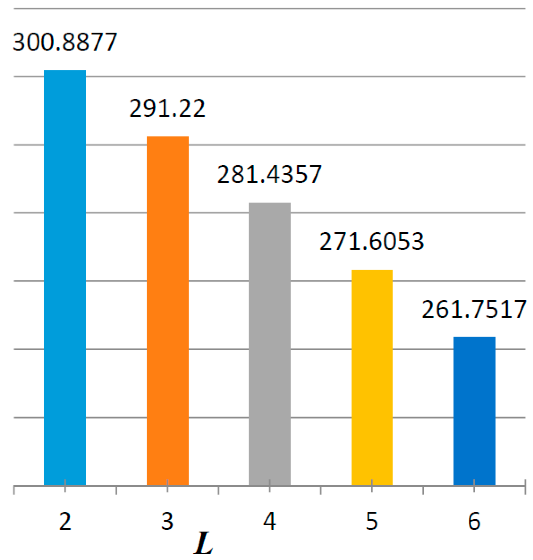
Figure 3.
The total expected profit of the retail chain with different λ.

Table 1.
Input parameters.
| Parameter | Value | Parameter | Value |
|---|---|---|---|
| a | 7.92 | q0 | 0.95 |
| b | 4.86 | θ | 0.85 |
| c | 3 | λ | 0.01 |
| d | 4.86 | m | 0.9 |
| f | 4 | t0 | 60 |
| T | 72 | L | 4 |
Table 2.
The optimal solutions with different θ.
| θ | ng | p | Q |
|---|---|---|---|
| 0.8 | 1.94 | 2.29 | 400.44 |
| 0.85 | 1.90 | 2.27 | 395.62 |
| 0.9 | 1.86 | 2.24 | 391.11 |
| 0.95 | 1.81 | 2.21 | 386.90 |
Table 3.
The optimal solution with different λ.
| λ | ng | p | Q |
|---|---|---|---|
| 0.005 | 2.05 | 2.37 | 341.25 |
| 0.01 | 1.90 | 2.27 | 281.44 |
| 0.015 | 1.78 | 2.18 | 236.96 |
| 0.02 | 1.68 | 2.12 | 203.38 |
| 0.025 | 1.60 | 2.06 | 177.63 |
Table 4.
Input parameters.
| Parameter | Value | Parameter | Value |
|---|---|---|---|
| ai | 7.92, 6.73, 9.79, 8.32 | q0i | 0.95, 0.92, 0.95, 0.97 |
| bi | 4.86, 4.13, 1.83, 1.56 | θi | 0.85, 0.8, 0.75, 0.9 |
| ci | 3, 2.5, 2.1, 1.9 | λi | 0.01, 0.02, 0.0067, 0.0067 |
| di | 4.86, 4.13, 1.83, 1.56 | e | 0.1 |
| fi | 3, 4, 5, 5 | t0i | 60, 60, 168, 168 |
| Ti | 72, 72, 240, 240 | Li | 6, 5, 10, 8 |
Table 5.
The results of the multi-item retail chain with different S.
| Capacity (S) | Total Profit Per Unit Time (П) | Shelf Space Cost (m) | Item | Price (pi) | Shelf Space (ngi) | Order Quantity (Qi) | Item Profit Per Unit Time (πi) |
|---|---|---|---|---|---|---|---|
| 10 | 38.74 | 0.9729 | 1 | 2.26 | 1.95 | 393.26 | 6.64 |
| 2 | 2.08 | 1.13 | 237.05 | 2.05 | |||
| 3 | 7.15 | 3.93 | 1370.30 | 18.60 | |||
| 4 | 6.65 | 2.98 | 1045.02 | 11.45 | |||
| 15 | 62.82 | 0.7960 | 1 | 2.50 | 2.83 | 470.75 | 9.69 |
| 2 | 2.20 | 1.57 | 268.80 | 2.91 | |||
| 3 | 8.18 | 6.18 | 1740.03 | 32.32 | |||
| 4 | 7.30 | 4.42 | 1268.04 | 17.91 | |||
| 20 | 93.02 | 0.7084 | 1 | 2.72 | 3.65 | 542.53 | 12.98 |
| 2 | 2.30 | 1.94 | 295.67 | 3.71 | |||
| 3 | 9.30 | 8.60 | 2140.30 | 51.01 | |||
| 4 | 7.93 | 5.81 | 1483.20 | 25.32 |
© 2017 by the authors. Licensee MDPI, Basel, Switzerland. This article is an open access article distributed under the terms and conditions of the Creative Commons Attribution (CC BY) license (http://creativecommons.org/licenses/by/4.0/).
Share and Cite
MDPI and ACS Style
Yang, S.; Xiao, Y.; Kuo, Y.-H. The Supply Chain Design for Perishable Food with Stochastic Demand. Sustainability 2017, 9, 1195. https://doi.org/10.3390/su9071195
AMA Style
Yang S, Xiao Y, Kuo Y-H. The Supply Chain Design for Perishable Food with Stochastic Demand. Sustainability. 2017; 9(7):1195. https://doi.org/10.3390/su9071195
Chicago/Turabian StyleYang, Shuai, Yujie Xiao, and Yong-Hong Kuo. 2017. "The Supply Chain Design for Perishable Food with Stochastic Demand" Sustainability 9, no. 7: 1195. https://doi.org/10.3390/su9071195
Note that from the first issue of 2016, this journal uses article numbers instead of page numbers. See further details here.