An Improved Eco-Efficiency Analysis Framework Based on Slacks-Based Measure Method

Abstract

The level of sustainable development can be measured by eco-efficiency, which is a combination of economic and ecological performance. Utilizing the weighted sum of the improved proportions of the indicators as the objective function, this paper develops a proportional slacks-based measure model to assess eco-efficiency, in which the conventional inputs, and desirable and undesirable outputs are improved to different proportions along the elements of a given directional vector. Moreover, this paper presents a weighted proportional slacks-based measure model using the ranges as the divisors instead of the input and output values in the objective function. Finally, this paper presents an empirical analysis by applying proposed measure models with the data of 30 provinces in China in 2015. The empirical study results indicate the developed slacks-based measure models can be used in the assessment of eco-efficiency effectively and reasonably.

1. Introduction

In the contemporary era, more and more nations in the world are paying attention to the global environmental problem such as the lack of resources, air and water pollution, global warming and climate change, and acid substance precipitation on Earth’s surface, which threaten the survival of human. Since it contains some ecological problems, environmental problem has become a major policy issue in the world. Any single nation cannot solve the ecological problems. Therefore, they need to be solved by international cooperation and the effort of all nations. In this aspect, environmental management and protection play an important role. In environmental protection, less resource consumption and waste emission are the most significant issues. Due to the shortage of resources and serious pollution, more and more countries give more emphasis to environmental protection while developing economy. The world has entered an era of ecological constraint. Sustainable development has become a consensus. The need for sustainable development has become crucial to improve environment and increase the earth’s carrying capacity. Sustainable development is an environmentally friendly, economically feasible and socially acceptable growth pattern. It is defined as “the development that meets the needs of the present without compromising the ability of future generations to meet their own needs” [1]. In this aspect, it is crucial to assess the environmental burdens to realize the objectives of sustainable development. Therefore, any nation (or region and organization) that strives for sustainable development has to measure its economic as well as environmental (ecological) efficiency.

The concept of economic–ecological efficiency, commonly known as eco-efficiency (EE), has been given more and more attention from researchers, government and so on. Economic–ecological efficiency was first introduced as a business link to sustainable development by Schaltegger and Sturm [2]. Afterwards, the Organization for Economic Cooperation and Development (OECD) [3] defined eco-efficiency as a ratio between the economic value of what has been produced and the environmental impact of the products or services. The World Business Council for Sustainable Development [4] utilized the notion of eco-efficiency as an approach of encouraging firms to become more competitive and simultaneously less contaminative. Eco-efficiency is a necessary but not a sufficient condition for achieving sustainability. Monitoring eco-efficiency is useful in order to make firms accountable to sustainability In addition, it is noted that environmental proactivity also has great influence on decreasing environmental pressures (resource consumption and waste emission) and improving eco-efficiency [5]. Because the increased eco-efficiency might offer a route towards sustainable development, the improvement of eco-efficiency is an efficient way of decreasing environmental pressures. Moreover, policies that target at improvements of eco-efficiency are easier to adopt than policies that aim at restricting the level of economic activity. Hence, measurement of eco-efficiency is very essential for sustainable development.

In the past 20 years, many scholars have developed models and methods for assessing eco-efficiency, such as simple ration approach [6], analytic hierarchy process method (AHP) [7], entropy weight method [8], grey relational analysis method [9], data envelopment analysis (DEA) [10,11,12,13,14,15] and so on. Apart from the above approaches, the systematic method based on self-checking system has been mentioned as more efficient for measuring the firm’s environmental performance. The method is applied to the environmental efficiency analysis of the food sector. It mitigates efficiently environmental problems and optimizes associated costs [16]. Because Eco-efficiency refers to the ability of industries, companies and regions to produce more goods and services with fewer resources as well as less waste emission, eco-efficiency was initially evaluated by simple ratio indicators such as GDP over SO₂, GDP over energy consumption at macro-level, or output per unit of waste at micro-level. These simple ratios can be easily understood by the policymakers and public. However, the simple indicators measure economic output per units of waste, and explain eco-efficiency from a very limited perspective.

Data envelopment analysis is an effective non-parametric approach for assessing the relative efficiency of a number of homogeneous decision making units (DMUs) [17]. In data envelopment analysis (DEA), there are various efficiency measure methods, such as radial measure [10,12,14,18,19], directional distance function measure [13,20,21,22,23,24,25,26,27], non-radial measure [28,29] and so on. These DEA methods do not take into account the impacts of the slacks on the efficiency assessment. However, the slack is a vital factor of the inefficiency.

For providing slacks-based efficiency measures, Charnes et al. [30] proposed an additive model that maximized the sum of both input and output slacks. Based on the directional distance function and additive model, Cooper et al. [31] also presented range-adjusted measure (RAM) of inefficiency. In RAM model, the objective function is the mean of the ratio of the slacks of inputs and outputs to their ranges. Tone [32] put forward a slacks-based measure (SBM) of efficiency. SBM is a nonlinear fractional programming problem, and the efficiency value of SBM was interpreted as the product of input and output inefficiencies. Hua et al. [11] considered the slacks, and proposed a different proportion measure model to evaluate the eco-efficiency of paper mills along the Huai River in China. Fukuyama and Weber [33] proposed a directional SBI (slacks-based inefficiency) measure model that incorporates all the sources of inefficiency, and relates to the directional distance function. Fukuyama and Weber [34] put forward a two-stage slacks-based inefficiency measure model to assess the performance of DMUs. It can account for any input and output slack of a network structure of production. Inputs in a first stage produce intermediate outputs, which are transformed to final outputs in the second stage. In addition, in order to overcome the lack of indication of the directional distance function measure model, Gómez-Calvet et al. [35] took into account non-directional slack and presented a second stage directional distance function measure model for assessing eco-efficiency. The efficiency value is the sum between the efficiency obtained in the first stage and an average mean of the relative non-directional slacks. The model provides a comprehensive performance measure. The model of Hua et al. [11] does not include the improved proportions of the resource inputs in the eco-efficiency formulation. In the directional SBI measure model of Fukuyama and Weber [33], the undesirable outputs are not considered. Thus, this paper develops a proportional slacks-based measure (PSBM) model to assess eco-efficiency. In this model, conventional inputs, and desirable and undesirable outputs are improved to different proportions along the elements of a given directional vector. The objective function is the weighted sum of the improved proportions of the indicators.

Moreover, following the weighted ideas of the MSBM of Sharp et al. [36] using the SP [23] ranges as the divisors instead of the input and output values in the objective function, this paper also presents a weighted proportional slacks-based measure model.

In this paper, the proposed measure models are related to the directional distance function and take into account all slacks of the input, and desirable and undesirable outputs in the evaluation of the EE. Eco-efficiency means that decision making units utilize fewer resources to produce more goods (or services) and emit less pollutants. Hence, it is reasonable to consider the resource inputs, desirable outputs and undesirable outputs (pollutants) simultaneously in the assessment of eco-efficiency.

The rest of this paper is organized as follows. In Section 2, based on previous works, we develop a slacks-based model and weighted model for eco-efficiency analysis. Then, the properties of the models are provided. We present an empirical illustration, using the data of 30 provinces in China for the year 2015. The computation results are analyzed in Section 3. Section 4 presents some conclusions and remarks.

2. Models

2.1. The Directional Distance Function Measure (DDFM) Model and Some Slacks-Based Models for Eco-Efficiency Evaluation

This section reviews the DDFM model and some slacks-based models.

There are J DMUs, denoted by DMUj (j = 1, 2, …, J). During production process, each DMUj (j = 1, 2, …, J) transforms inputs x_ij (i = 1, 2, …, I) (resource) into desirable outputs y_mj (m = 1, 2, …, M) and undesirable outputs z_lj (l = 1, 2, …, L) (residuals and pollutants). x_ij, y_mj and z_lj are supposed to be positive.

In accordance with earlier papers [10,11,12,13], we treat undesirable outputs (pollutants) as conventional inputs. Let λ_j ≥ 0, j = 1, 2, …, J be the intensity variables, and then the technology structure is represented as:

$$\begin{array}{l}T=\{(x_1,x_2,\cdots ,x_I,y_1,y_2,\cdots ,y_M,z_1,z_2,\cdots ,z_L):\\ {\displaystyle \sum _{j=1}^J{\lambda }_j{x}_{ij}}\le x_i,i=1,2,\cdots ,I\\ {\displaystyle \sum _{j=1}^J{\lambda }_j{y}_{mj}}\ge y_m,m=1,2,\cdots ,M\\ {\displaystyle \sum _{j=1}^J{\lambda }_j{z}_{lj}}\le z_l,l=1,2,\cdots ,L\\ {\lambda }_j\ge 0,j=1,2,\cdots ,J.\}\end{array}$$

The eco-efficiency is defined as a ratio of a weighted sum of desirable outputs to a weighted sum of environmental pressure:

Eco-efficiency = desirable output/environmental pressure

Environmental pressure includes inputs (resources) and the discharge of residuals and pollutants [12]. The desirable outputs include GDP, goods, services, etc. Eco-efficiency aims at achieving more desirable outputs with fewer resource inputs and emitting fewer pollutants.

Let $g=(-g_x,g_y,-g_z),g_x\in {\Re }_{+}^I,g_y\in {\Re }_{+}^M$ and $g_z\in {\Re }_{+}^L$ be a directional vector, which leads to the following directional distance function (DDF)

$$\stackrel{\rightharpoonup }{D}[x,y,z;g=(-g_x,g_y,-g_z)]=Sup[\beta |(x-\beta g_x,y+\beta g_y,z-\beta g_z)\in T].$$

(1)

According to Equation (1) and the technology structure T, the eco-efficiency $E{E}_k^{A1}$ is computed by the following directional distance function measure model [22]:

$$\begin{array}{l}E{E}_k^{A1}=\max \beta \\ s.t.{\displaystyle \sum _{j=1}^J{\lambda }_j{x}_{ij}}\le x_{ik}-\beta g_{x_i},i=1,2,\cdots ,I\\ {\displaystyle \sum _{j=1}^J{\lambda }_j{y}_{mj}}\ge y_{mk}+\beta g_{y_m},m=1,2,\cdots ,M\\ {\displaystyle \sum _{j=1}^J{\lambda }_j{z}_{lj}}\le z_{lk}-\beta g_{z_l},l=1,2,\cdots ,L\\ {\lambda }_j\ge 0,j=1,2,\cdots ,J.\end{array}$$

(2)

where $g_x\in {\Re }_{+}^I,g_y\in {\Re }_{+}^M$ and $g_z\in {\Re }_{+}^L$.

The above Model (2) can be presented in the following mode:

$$(\mathrm{DDFM})\begin{array}{l}E{E}_k^{A1}=\max \beta \\ s.t.{\displaystyle \sum _{j=1}^J{\lambda }_j{x}_{ij}}+t_i^{-}=x_{ik}-\beta g_{x_i},i=1,2,\cdots ,I\\ {\displaystyle \sum _{j=1}^J{\lambda }_j{y}_{mj}}-d_m^{+}=y_{mk}+\beta g_{y_m},m=1,2,\cdots ,M\\ {\displaystyle \sum _{j=1}^J{\lambda }_j{z}_{lj}}+p_l^{-}=z_{lk}-\beta g_{z_l},l=1,2,\cdots ,L\\ {\lambda }_j,t_i^{-},d_m^{+},p_l^{-}\ge 0,\forall j,i,m,l.\end{array}$$

(3)

where $\beta ,{\lambda }_j$ are the objective value and weight, $t_i^{-},p_l^{-}$ and $d_m^{+}$ are non-directional slacks of the inputs, and undesirable and desirable outputs, and $g_x\in {\Re }_{+}^I,g_y\in {\Re }_{+}^M$ and $g_z\in {\Re }_{+}^L$.

Let an optimal solution of Model (3) be $({\beta }^{\ast },{\lambda }^{\ast },t^{-\ast },d^{+\ast },p^{-\ast })$. Here $t^{-\ast }=(t_1^{-\ast },t_2^{-\ast },\cdots ,t_I^{-\ast }),p^{-\ast }=(p_1^{-\ast },p_2^{-\ast },\cdots ,p_L^{-\ast })$ and $d^{+\ast }=(d_1^{+\ast },d_2^{+\ast },\cdots ,d_M^{+\ast })$ are non-directional slack vectors, and ${\lambda }^{\ast }=({\lambda }_1^{\ast },{\lambda }_2^{\ast },\cdots ,{\lambda }_J^{\ast })$ is the weight vector. In Model (3), the DMUk is efficient if the eco-efficiency $E{E}_k^{A1}({\beta }^{\ast })$ is equal to zero. If eco-efficiency $E{E}_k^{A1}$ is greater than zero (β* > 0), the DMUk is inefficient.

In DDFM model, the projection point determined by the directional vector may not belong to the strongly efficient frontier. If weakly efficient units are chosen as benchmarks, the efficiency value does not reflect the true amount of slack (compared to the strongly efficient frontier) [37]. Directional slack is relative to the weakly efficient frontier and it is the improved amount of inputs and outputs along a given directional vector. Directional slack is the product between the efficiency value of DDFM model and the directional vector element. Apart from the directional slack, non-directional slack, which is the difference between the total slack amount and the directional slack in DDFM model, should be considered for a comprehensive inefficiency measure [38].

Directional distance function measure models have better economic and proportional interpretations of efficiency. The economic interpretation of DDFM depends on the chosen directional vector g = (−g_x, g_y, −g_z). The parameter β measures the proportion by which the desirable outputs could be increased while the inputs and undesirable outputs are contracted in the same proportion along a given directional vector. The directional distance function inflates desirable outputs in the g_y direction, decreases undesirable outputs in the −g_z direction, and reduces inputs in the −g_x direction, while remaining within the technology set. Radial measure assumes that contraction of inputs and undesirable outputs, or augmenting desirable outputs, are of the same proportion. However, DDFM model can handle the inputs, undesirable outputs and desirable outputs simultaneously. The directional distance is calculated by programming model. When the vector of the observed variables is defined for optimization, the efficiency value is in the [0, 1] interval. In this model, zero is the benchmark for the efficient frontier. In addition, DDFM model is flexible in choosing the projection direction. However, it has a disadvantage due to the lack of indication [38]. The reason is that the projection point determined by the directional vector may not be on the strongly efficient frontier. A weakly efficient frontier point does not take into account the true amount of slacks. Hence, the inefficiency value in the DDFM model is underestimated [35].

In this paper, it is supposed that technology exhibits constant returns to scale, by allowing the sum of the elements of intensity vector to be free for the following reasons: First, ecological perspective and economic activity are commonly characterized by the constant returns to scale since what really matters from this view is the inputs and undesirable outputs exerted on the environment and not their distribution among different regions [39]. The constant returns to scale approach was used in previous papers, including Kuosmanen and Kortelainen [40]. Second, accounting for variable returns to scale in the computation of radial scores of eco-efficiency is straightforward. However, it is difficult to consider this assumption for the non-radial measure model of eco-efficiency in this paper [13]. Torgersen et al. [41] pointed out that we prefer to leave the scale measures as radial concepts. The idea of measuring technical efficiency by a radial measure model stems from Farrel [42], in which the inputs are reduced at the same proportion, while remaining in the production possible set. Torgerser et al. [41] decomposed Farrell’s original measure into separate measures of scale efficiency and technical efficiency. Scale measures are derived from the radial measure model. Forsund and Hjalmarsson [43] and Banker et al. [44] implemented it for linear technology. Third, the size of the firm or production activity does not matter in the assessment of eco-efficiency, since we are only interested in the ratio of the desirable outputs to the environmental pressure (resource inputs and pollutant emissions).

2.2. The Proportional Slacks-Based Measure Model (PSBM)

In this section, a proportional slacks-based measure (PSBM) model is developed.

Evidently, the DDFM model assesses relative efficiency. It increases the desirable outputs and decreases the inputs and undesirable outputs simultaneously by the same proportion, along a given directional vector g = (−g_x, g_y, −g_z). However, after attaining the maximum reduced (increased) proportion β* of the direction of inputs and undesirable outputs (desirable outputs), additional contraction (augmentation) may still be feasible in some inputs and undesirable outputs (desirable output) because of non-directional slacks. The DDFM model does not consider all possible sources of inefficiency.

Hua et al. [11] put forward a program model as:

$$\begin{array}{l}E{E}_k=\max \left[\left(\frac{1}{M}{\displaystyle \sum _{m=1}^M{\theta }_m}+\frac{1}{L}{\displaystyle \sum _{l=1}^L{\delta }_l}\right)\right]\\ s.t.{\displaystyle \sum _{j=1}^J{\omega }_j{x}_{ij}}=x_{ik}-r_i^{-},i=1,2,\cdots ,I\\ {\displaystyle \sum _{j=1}^J{\omega }_j{y}_{mj}}={\theta }_m{y}_{mk},m=1,2,\cdots ,M\\ {\displaystyle \sum _{j=1}^J{\omega }_j{z^{\prime }}_{lj}={\delta }_l}{z^{\prime }}_{lk},l=1,2,\cdots ,L\\ {\omega }_j,r_i^{-}\ge 0,\forall j,i\\ {\theta }_m\ge 1,{\delta }_l\ge 1,\forall m,l\end{array}$$

(4)

where ${z^{\prime }}_{lk}$ is the transformed undesirable output, and y_mk is the desirable output.

The model of Hua et al. [11] increased desirable output and transformed undesirable output to different proportions. Let $({\omega }_j^{\ast },{\theta }_m^{\ast },{\delta }_l^{\ast })$ be the optimal solution of the above model. ${\displaystyle \sum _{j=1}^J{\omega }_j^{\ast }{y}_{mj}}$ and ${\displaystyle \sum _{j=1}^J{\omega }_j^{\ast }{z^{\prime }}_{lj}}$ generate a point on the efficiency frontier. Then, we have ${\displaystyle \sum _{j=1}^J{\omega }_j^{\ast }{y}_{mj}}={\theta }_m^{\ast }{y}_{mk},{\displaystyle \sum _{j=1}^J{\omega }_j^{\ast }{z^{\prime }}_{lj}}={\delta }_l^{\ast }{z^{\prime }}_{lk}$. Hence, ${\theta }_m^{\ast }=\frac{{\displaystyle \sum _{j=1}^J{\omega }_j^{\ast }{y}_{mj}}}{y_{mk}},{\delta }_l^{\ast }=\frac{{\displaystyle \sum _{j=1}^J{\omega }_j^{\ast }{z^{\prime }}_{lj}}}{{z^{\prime }}_{lk}}$ are the ratio between the values of efficiency frontier and the observed desirable outputs and transformed undesirable outputs. The objective function in Model (4) is directed to maximize a weighted average of these ratios. ${\theta }_m^{\ast }{y}_{mk},{\delta }_l^{\ast }{z^{\prime }}_{lk}$ are efficient values, which represent the necessary amount of each desirable output and transformed undesirable output that need to be obtained. The efficiency measure is confined to output inefficiencies.

Fukuyama and Weber [33] proposed a directional slacks-based inefficiency (SBI) measure model of inefficiency as:

$$(\mathrm{SBI})\begin{array}{l}E{E}_k=\max \left[\frac{1}{2}\left(\frac{1}{I}{\displaystyle \sum _{i=1}^I\frac{r_i^{-}}{g_{x_i}}}+\frac{1}{M}{\displaystyle \sum _{m=1}^M\frac{s_m^{+}}{g_{y_m}}}\right)\right]\\ s.t.{\displaystyle \sum _{j=1}^J{\omega }_j{x}_{ij}}=x_{ik}-r_i^{-},i=1,2,\cdots ,I\\ {\displaystyle \sum _{j=1}^J{\omega }_j{y}_{mj}}=y_{mk}+s_m^{+},m=1,2,\cdots ,M\\ {\omega }_j,r_i^{-},s_m^{+}\ge 0,\forall j,i,m\end{array}$$

where $g_x\in {\Re }_{+}^I,g_y\in {\Re }_{+}^M$.

Let $({\omega }_j^{\ast },r_i^{-\ast },s_m^{+\ast })$ be the optimal solution of SBI model. Then, $r_i^{-\ast }=x_{ik}-{\displaystyle \sum _{j=1}^J{\omega }_j^{\ast }{x}_{ij}},s_m^{+\ast }={\displaystyle \sum _{j=1}^J{\omega }_j^{\ast }{y}_{mj}}-y_{mk}$ denote the inefficiencies of the inputs and outputs. $\frac{r_i^{-\ast }}{g_{x_i}}$ and $\frac{s_m^{+\ast }}{g_{y_m}}$ represent the ratio between the inefficiency value of the indicator and the directional vector elements. $\frac{1}{2I{g}_{x_i}}$ and $\frac{1}{2M{g}_{y_m}}$ may also be regarded as the relative weights to be assigned to the inefficiencies. The weights represent value judgment [31]. The objective function is to maximize the weighted average of the input and output slacks.

Directional SBI measure model incorporates all the sources of inefficiency. Moreover, it is related to the direction distance function, and generalizes some measures. Its computation is not complex. Based on Model (4) and directional SBI measure model, we consider the inputs, desirable outputs and undesirable outputs simultaneously, and propose a proportional slacks-based measure model as:

$$(\mathrm{PSBM})\begin{array}{l}E{E}_k^{A2}=\max \left[\frac{1}{I+M+L}\left({\displaystyle \sum _{i=1}^I{\alpha }_i}+{\displaystyle \sum _{m=1}^M{\theta }_m}+{\displaystyle \sum _{l=1}^L{\delta }_l}\right)\right]\\ s.t.{\displaystyle \sum _{j=1}^J{\omega }_j}{x}_{ij}=x_{ik}-{\alpha }_i{g}_{x_i},i=1,2,\cdots ,I\\ {\displaystyle \sum _{j=1}^J{\omega }_j{y}_{mj}}=y_{mk}+{\theta }_m{g}_{y_m},m=1,2,\cdots ,M\\ {\displaystyle \sum _{j=1}^J{\omega }_j{z}_{lj}}=z_{lk}-{\delta }_l{g}_{z_l},l=1,2,\cdots ,L\\ {\omega }_j,{\alpha }_i,{\theta }_m,{\delta }_l\ge 0,\forall j,i,m,l.\end{array}$$

(5)

where $g_x\in {\Re }_{+}^I,g_y\in {\Re }_{+}^M$ and $g_z\in {\Re }_{+}^L$.

Let $({\rho }^{\ast },{\omega }_j^{\ast },{\alpha }_i^{\ast },{\theta }_m^{\ast },{\delta }_l^{\ast })$ be the optimal solution of Model (5). ${\alpha }_i^{\ast }$ is the proportion of input $i$, which can be decreased by in the $-g_x$ direction. ${\delta }_l^{\ast }$ is the reduced proportion of undesirable output $l$, in the $-g_z$ direction. ${\theta }_m^{\ast }$ is the expanded proportion of desirable output $m$, in the $g_y$ direction.

In Model (5), the DMU is efficient if the eco-efficiency $E{E}_k^{A2}({\rho }^{\ast })$ is equal to zero. If $E{E}_k^{A2}>0$ (any of ${\alpha }_i^{\ast },{\theta }_m^{\ast },{\delta }_l^{\ast }$ is greater than zero), then the DMU is inefficient.

In PSBM model, the directional vector represents value judgments that are not included in the data of inputs and outputs. Different managers may use various values as a guide to choice. The directional vectors based on data are usually utilized. $(-x_i,y_m,-z_l)$ is the direction of the observed indicators. The range of a variable is defined as its maximum observed minus its minimum observed value. In such a range, worst performance is given by maximum inputs and minimum desirable outputs. This is because worst performance is included in the definition of the range, and efficiency results depending on the range defined [31]. For Model (5), under the constraint ${\displaystyle \sum _{j=1}^J{\lambda }_j}=1$, we have

$$\begin{array}{l}{s}_i^{-}={\alpha }_i{g}_{x_i}=x_{ik}-{\displaystyle \sum _{j=1}^J{\omega }_j{x}_{ij}}\le \underset{j}{\max }(x_{ij})-\underset{j}{\min }(x_{ij})\\ d_m^{+}={\theta }_m{g}_{y_m}={\displaystyle \sum _{j=1}^J{\omega }_j{y}_{mj}}-y_{mk}\le \underset{j}{\max }(y_{mj})-\underset{j}{\min }(y_{mj})\\ p_l^{-}={\delta }_l{g}_{z_l}=z_{lk}-{\displaystyle \sum _{j=1}^J{\omega }_j{z}_{lj}}\le \underset{j}{\max }(z_{lj})-\underset{j}{\min }(z_{lj})\end{array}$$

Thus, the evaluation results are relative to the maximum inefficiency, which the observations allow in each input and output. When $s_i^{-\ast }=\underset{j}{\max }(x_{ij})-\underset{j}{\min }(x_{ij})$, $x_{ik}$ for DMUk, is equal to $\underset{j}{\max }(x_{ij})$, the worst observed value for this input. When $p_l^{-\ast }=\underset{j}{\max }(z_{lj})-\underset{j}{\min }(z_{lj})$, $z_{lk}$ for DMUk, is equal to $\underset{j}{\max }(z_{lj})$, the worst observed value for this undesirable output. When $d_m^{+\ast }=\underset{j}{\max }(y_{mj})-\underset{j}{\min }(y_{mj})$, for $y_{mk}$ is equal to $\underset{j}{\min }(y_{mj})$, the worst desirable output [31]. In the empirical analysis, the directional vector of the input and output and range directional vector are based on data.

2.3. The Weighted PSBM Model (WPSBM)

Based on this PSBM, a weighted PSBM model is provided in this section.

In the proposed PSBM Model (5), the weight $\frac{1}{I+M+L}$ of the objective function does not take into account the economic importance of proportions ${\alpha }_i(i=1,2,\cdots ,I),{\theta }_m(m=1,2,\cdots ,M)$ and ${\delta }_l(l=1,2,\cdots ,L)$, since the same weight is assigned to the proportion in each element of a given directional vector. If faced with any institutional constraint, such as government regulations, the decision makers may wish to assign different priorities to the slacks.

Sharp et al. [36] put forward a modified slacks-based measure (MSBM) model. Liu and Tone [45] presented a weighted slacks-based measure (WSBM) model. The MSBM and WSBM models can account for managerial preferences. Following the weighted ideas of the MSBM and WSBM models, we set up a weighted PSBM model as:

$$(\mathrm{WPSBM})\begin{array}{l}E{E}_k^{A3}=\max \left[\frac{1}{I+M+L}\left({\displaystyle \sum _{i=1}^I{u}_i{\alpha }_i}+{\displaystyle \sum _{m=1}^M{v}_m{\theta }_m}+{\displaystyle \sum _{l=1}^L{q}_l{\delta }_l}\right)\right]\\ s.t.{\displaystyle \sum _{j=1}^J{\omega }_j}{x}_{ij}=x_{ik}-{\alpha }_i{g}_{x_i},i=1,2,\cdots ,I\\ {\displaystyle \sum _{j=1}^J{\omega }_j{y}_{mj}}=y_{mk}+{\theta }_m{g}_{y_m},m=1,2,\cdots ,M\\ {\displaystyle \sum _{j=1}^J{\omega }_j{z}_{lj}}=z_{lk}-{\delta }_l{g}_{z_l},l=1,2,\cdots ,L\\ {\displaystyle \sum _{i=1}^I{u}_i}+{\displaystyle \sum _{m=1}^M{v}_m}+{\displaystyle \sum _{l=1}^L{q}_l}=I+M+L\\ {\omega }_j,{\alpha }_i,{\theta }_m,{\delta }_l\ge 0,\forall j,i,m,l\\ u_i,v_m,q_l>0,\forall i,m,l.\end{array}$$

(6)

where $\frac{u_i}{I+M+L},\frac{v_m}{I+M+L},\frac{q_l}{I+M+L}({\displaystyle \sum _{i=1}^I{u}_i}+{\displaystyle \sum _{m=1}^M{v}_m}+{\displaystyle \sum _{l=1}^L{q}_l}=I+M+L)$ are, respectively, the weights assigned to the proportions ${\alpha }_i,{\theta }_m,{\delta }_l$ for the direction of input $i$, desirable output $m$ and undesirable output $l$, and $g_x\in {\Re }_{+}^I,g_y\in {\Re }_{+}^M,g_z\in {\Re }_{+}^L$. WPSBM model allows us to alter the proportion’s weights in the objective function.

In WPSBM model, the slacks of the input, undesirable output and desirable output are, respectively, defined as $s_i^{-}={\alpha }_i{g}_{x_i},r_l^{-}={\delta }_l{g}_{z_l},t_m^{+}={\theta }_m{g}_{y_m}$. They represent the reduced (expanded) amount of the input and undesirable output (desirable output). They are the total amount of slack. Slack is a vital source of inefficiency. WPSBM model considers the impact of the true amount of slacks on eco-efficiency. Hence, it overcomes the “lack of indication” of DDFM model.

Let $({\gamma }^{\ast },{\omega }_j^{\ast },{\alpha }_i^{\ast },{\theta }_m^{\ast },{\delta }_l^{\ast })$ be the optimal solution of Model (6). ${\alpha }_i^{\ast },{\theta }_m^{\ast },{\delta }_l^{\ast }$ is the improved proportion of the indicators along a given directional vector. The objective function is to maximize the weighted average of these proportions, and the directional vector reflects the value judgment of the decision-makers. In addition, according to the economic importance of each indicator, decision-makers may provide the weight of proportions of indicators in the objective function.

Eco-efficiency ${\gamma }^{\ast }$ of WPSBM model appears intuitively likely to be greater than the eco-efficiency ${\beta }^{\ast }$ of DDFM model, for a given directional vector. The reason is that all the inputs and outputs in DDFM model are improved by the same proportion $\beta$, and WPSBM model consider the impact of slacks on the eco-efficiency. The following part gives the properties of WPSBM model.

Property 1.

For a given directional vector $g=(-g_x,g_y,-g_z),g_x\in {\Re }_{+}^I,g_y\in {\Re }_{+}^M$ and $g_z\in {\Re }_{+}^L$, eco-efficiency ${\gamma }^{\ast }$ of WPSBM model is greater than eco-efficiency ${\beta }^{\ast }$ of DDFM model.

Proof. 

Let an optimal solution of DDFM Model (3) be $({\beta }^{\ast },{\lambda }^{\ast },t^{-\ast },d^{+\ast },p^{-\ast })$. Here, ${\lambda }^{\ast }=({\lambda }_1^{\ast },{\lambda }_2^{\ast },\cdots ,{\lambda }_J^{\ast })$ is the weight vector, and $t^{-\ast }=(t_1^{-\ast },t_2^{-\ast },\cdots ,t_I^{-\ast }),p^{-\ast }=(p_1^{-\ast },p_2^{-\ast },\cdots ,p_L^{-\ast })$ and $d^{+\ast }=(d_1^{+\ast },d_2^{+\ast },\cdots ,d_M^{+\ast })$ are non-directional slack vectors. Then we have

$$\begin{array}{l}{\displaystyle \sum _{j=1}^J{\lambda }_j^{\ast }{x}_{ij}}=x_{ik}-{\beta }^{\ast }{g}_{x_i}-t_i^{-\ast },i=1,2,\cdots ,I\\ {\displaystyle \sum _{j=1}^J{\lambda }_j^{\ast }{y}_{mj}}=y_{mk}+{\beta }^{\ast }{g}_{y_m}+d_m^{+\ast },m=1,2,\cdots ,M\\ {\displaystyle \sum _{j=1}^J{\lambda }_j^{\ast }{z}_{lj}}=z_{lk}-{\beta }^{\ast }{g}_{z_l}-p_l^{-\ast },l=1,2,\cdots ,L.\end{array}$$

where $g_x\in {\Re }_{+}^I,g_y\in {\Re }_{+}^M,g_z\in {\Re }_{+}^L$.

Let us define

$$\begin{array}{l}{\omega }_j={\lambda }_j^{\ast },j=1,2,\cdots ,J\\ {\alpha }_i={\beta }^{\ast }+\frac{t_i^{-\ast }}{g_{x_i}},i=1,2,\cdots ,I\\ {\theta }_m={\beta }^{\ast }+\frac{d_m^{+\ast }}{g_{y_m}},m=1,2,\cdots ,M\\ {\delta }_l={\beta }^{\ast }+\frac{p_l^{-\ast }}{g_{z_l}},l=1,2,\cdots ,L.\end{array}$$

Then, $(\omega ,\alpha ,\theta ,\delta )$ is a feasible solution of the WPSBM Model (6). Here, $\omega =({\omega }_1,{\omega }_2,\cdots ,{\omega }_J)$ is the weight vector, and $\alpha =({\alpha }_1,{\alpha }_2,\cdots ,{\alpha }_I),\theta =({\theta }_1,{\theta }_2,\cdots ,{\theta }_M)$, and $\delta =({\delta }_1,{\delta }_2,\cdots ,{\delta }_L)$ are proportion vectors. The objective value of Model (6) is

$$\begin{array}{ll}\gamma & =\frac{1}{I+M+L}\left({\displaystyle \sum _{i=1}^I{u}_i}{\alpha }_i+{\displaystyle \sum _{m=1}^M{v}_m{\theta }_m}+{\displaystyle \sum _{l=1}^L{q}_l}{\delta }_l\right)\\ & =\frac{1}{I+M+L}\left[{\displaystyle \sum _{i=1}^I{u}_i\left({\beta }^{\ast }+\frac{t_i^{-\ast }}{g_{x_i}}\right)+{\displaystyle \sum _{m=1}^M{v}_m}\left({\beta }^{\ast }+\frac{d_m^{+\ast }}{g_{y_m}}\right)+{\displaystyle \sum _{l=1}^L{q}_l\left({\beta }^{\ast }+\frac{p_l^{-\ast }}{g_{z_l}}\right)}}\right]\\ & =\frac{{\displaystyle \sum _{i=1}^I{u}_i}+{\displaystyle \sum _{m=1}^M{v}_m}+{\displaystyle \sum _{l=1}^L{q}_l}}{I+M+L}{\beta }^{\ast }+\frac{1}{I+M+L}\left({\displaystyle \sum _{i=1}^I\frac{u_i{t}_i^{-\ast }}{g_{x_i}}+{\displaystyle \sum _{m=1}^M\frac{v_m{d}_m^{+\ast }}{g_{y_m}}}+{\displaystyle \sum _{l=1}^L\frac{q_l{p}_l^{-\ast }}{g_{z_l}}}}\right)\\ & ={\beta }^{\ast }+\frac{1}{I+M+L}\left({\displaystyle \sum _{i=1}^I\frac{u_i{t}_i^{-\ast }}{g_{x_i}}}+{\displaystyle \sum _{m=1}^M\frac{v_m{d}_m^{+\ast }}{g_{y_m}}}+{\displaystyle \sum _{l=1}^L\frac{q_l{p}_l^{-\ast }}{g_{z_l}}}\right)\ge {\beta }^{\ast }\end{array}$$

Since the optimal ${\gamma }^{\ast }$ of the objective function of Model (6) is greater than $\gamma$, we have ${\gamma }^{\ast }\ge {\beta }^{\ast }$. ☐

Property 2.

Let directional vector be $g=(-x_i,y_m,-z_l)$; when the weights in the objective function are given, WPSBM model is unit invariant, but it is not translation invariant.

Property 2 indicates that under $g=(-x_i,y_m,-z_l)$, efficiency measure of the WPSBM is invariant when the units of the inputs and outputs change. However, the optimal solution of WPSBM model changes while an amount is added to each indicator, namely parallel translation.

Property 3.

Let directional vector $g=(-g_x,g_y,-g_z),g_x\in {\Re }_{+}^I,g_y\in {\Re }_{+}^M$ and $g_z\in {\Re }_{+}^L$; where $g_{x_i}=\underset{j}{\max }(x_{ij})-\underset{j}{\min }(x_{ij}),g_{y_m}=\underset{j}{\max }(y_{mj})-\underset{j}{\min }(y_{mj})$, $g_{z_l}=\underset{j}{\max }(z_{lj})-\underset{j}{\min }(z_{lj})$. Then, when the weights in the objective function are given, WPSBM model is unit invariant, and it is translation invariant under the variable returns to scale (VRS), namely adding constraint ${\displaystyle \sum _{j=1}^J{\omega }_j}=1$.

Property 3 shows that efficiency measure of the WPSBM is unit invariant, when the directional vector is the range vector. It is the same as $g=(-x_i,y_m,-z_l)$. The WPSBM model is translation invariant under the variable returns to scale (VRS), when the directional vector is the range vector. One of the reasons is under VRS, and the other reason is that the range does not change with the addition of a constant to each input and output. Hence, the solution of WPSBM model does not change under the variable returns to scale (VRS) for parallel translation of the input and output.

There are some advantages to WPSBM model. First, it is a linear programming problem and is not complicated to solve. Second, it considers resource inputs, undesirable outputs and desirable outputs simultaneously, and it can assess eco-efficiency more accurately and comprehensively. Third, WPSBM model has a better economic proportion interpretation. It can directly provide the expanded (contracted) proportions of the desirable outputs (resource inputs and pollutant emissions). Fourth, it considers the impacts of the slacks on eco-efficiency values and encapsulates all possible sources of inefficiency. The computation results in the empirical analysis in Section 3 indicate that the influence of the slacks on eco-efficiency is very big, and cannot be neglected. In addition, it is related to the directional distance function, and is more general. This model is unit invariance when the unit of the directional vector is the same as the inputs and outputs. Moreover, WPSBM model allow decision-makers to take into account the economic importance of inputs and outputs in the assessment of eco-efficiency. Decision-makers may give weights of the proportions of indicators in the objective function according to the economic importance.

In the empirical analysis of Section 3, we use the DDFM, PSBM and WPSBM models to estimate eco-efficiency for two sets of directional vectors:

Directional vector 1:

$$g=(-g_x,g_y,-g_z)\mathrm{for}{g}_{x_i}=x_i(\forall i),g_{y_m}=y_m(\forall m),g_{z_l}=z_l(\forall l)$$

Directional vector 2:

$$g=(-g_x,g_y,-g_z)\mathrm{for}{g}_{x_i}=\underset{j}{\max }(x_{ij})-\underset{j}{\min }(x_{ij}),g_{y_m}=\underset{j}{\max }(y_{mj})-\underset{j}{\min }(y_{mj})$$

$$g_{z_l}=\underset{j}{\max }(z_{lj})-\underset{j}{\min }(z_{lj}),\forall i,m,l.$$

3. Empirical Analysis

In this section, we applied the DDFM model and the proposed PSBM and WPSBM models to analyze the eco-efficiency of 30 provinces in China in 2015.

3.1. Input and Output Indicators

In the physical economy, we input material, energy and produce products, and at the same time waste and emissions (other undesirable outputs) are unavoidable [12]. Hence, there are two essential classes of inputs from nature into the economy: the supply of resources (i.e., energy and water) and nature’s function as sink for the discharge of residuals and pollutants [12]. Mickwitz and Melanen [46] pointed out that environmental pressure (impact) indicators such as emissions, land use and resource extractions can be used to monitor the changes in environmental effects, since they are related to the total annual production volume of the regions.

Eco-efficiency is defined as a ratio between the economic value of what has been produced and the environmental impact of the products or services [3]. There are still no standard indicators and measurements for economic and environmental values [47]. Some institutions and researchers established economic value and environmental performance indicators. For the economic part of the eco-efficiency ratio, WBSCD selected quantity of goods (or services) and net sales as general indexes of product (or service) value, and value added as supplemental indicators [4]. United Nations Conference on Trade and Development (UNCTAD) suggested utilizing value added to represent economic performance indicators [48]. At the regional level, Seppala et al. [49] applied gross domestic product (GDP), value added of industries and output at the basic prices to represent the value of products and services in the Kymenlaakso region. In addition, GDP was also used to represent the values of products and services for analyzing eco-efficiency of cities in China [14], environmental efficiency of a regional economy [50], environmental efficiency of the 22 OECD countries [51] and environmental performance [52].

The environmental impact part of the eco-efficiency ratio includes resource inputs and the discharge of residuals and pollutants [12]. WCED [1] suggested selecting greenhouse gas (GHG) emissions, energy consumption, water withdrawals, and hazardous waste as environmental indicators. WBSCD [4] recommended taking material consumption, energy consumption, water consumption, ozone depleting substance emissions and greenhouse gas (GHG) emissions as five general applicable indicators, and acidification gas emissions and total waste as two supplemental indexes. Verfaillie et al. [53] thought that four environmental aspects dominated the overall environmental performance: global warming potential, photochemical oxidation potential, acidification potential and emissions of heavy metals. Global warming potential is influenced by carbon dioxide (CO₂), methane (CH₄) and other greenhouse gases. Sulfur dioxide (SO₂) and nitrogen oxide emissions contribute to acidification effect. Seppala et al. [49] divided environmental impact indicators into three sections: pressure indicators (such as emission of SO₂), impact category indicators (e.g., CO₂ equivalents in the case of climate change), and a total impact indicator. German environmental economic account took land input, energy consumption, water consumption, material consumption, labor input, capital input, greenhouse gas emissions and acid gas emissions as environmental pressure indicators in the assessment of eco-efficiency [6]. While referring to the regional environmental impact indicators, Mickwitz et al. [46] applied physical input–output tables of Kymenlaakso’s regional economy to obtain the natural resource consumption indicators, such as total material requirement or direct material input.

In some other literature, water consumption was taken as one of the input indicators for assessing eco-efficiency [6,12,14,54,55]. Energy consumption was selected as one of the input indicators for analyzing eco-efficiency [12,14]. Since the construction land area represents land utilization, it was considered as one of the input indicators for measuring eco-efficiency [6,14,46,54]. Chemical oxygen demand (COD) emissions, SO₂ emissions, and soot and dust emissions were chosen as some undesirable output indicators for analyzing eco-efficiency [12,14,54]. In addition, Mahlberg and Sahoo [51] took the greenhouse gas as the undesirable output to measure environmental efficiency of the 22 OECD countries. Zhang et al. [12] chose solid waste as one of the undesirable outputs to assess eco-efficiency of industrial system in China.

Sorvari et al. [56] indicated eco-efficiency can also be understood as a wider notion including social and cultural aspects. Mickwitz et al. [46] presented the social and cultural indicator “safety” (which is measured by the development of certain crimes, the number of violent crime and the number of traffic accidents). Some studies took labor as one of the input indicators. The number of employed persons can represent a region’s stability, prosperity and vitality [57]. Mahlberg and Sahoo [51] found labor is one of the most important inputs, and considered the social indicator (labor) for eco-efficiency analysis of the 22 OECD countries. Some other studies also selected labor as an input indicator to measure eco-efficiency [6,14,54,58,59]. In addition to the above studies, the number of employees was selected as one of the inputs for the analysis of the operational and environmental assessment of Japanese electric power companies [60]. Whether the numbers of employed person should be utilized as an input or output depends on the research purpose [14]. However, one goal of economic development is to improve labor productivity. Moreover, eco-efficiency aims at producing more goods and services with fewer resources as well as less waste emissions. Hence, this paper also takes the labor as an input indicator to measure its contribution to the desirable outputs.

Based on previous studies, considering the data availability, this research establishes nine indicators for assessing the eco-efficiency of 30 provinces in China in 2015. For the desirable output, the gross domestic production (GDP) is usually used. This paper uses GDP at a regional level as a measure of economic value of a regional economy. For the resource inputs, according to the material flow accounts, taking into account the social factor (labor), four main categories of resource input indicators are finally selected in this research: water resource consumption, construction land, employment population and energy consumption. These indicators reflect the contributions to the desirable output. For undesirable outputs, COD, nitrogen oxide, sulfur dioxide (SO₂) and soot and dust are finally selected in the research. In China, in recent years, driven by sustained and rapid growth of industrial, agricultural and municipal pollutants, water and air quality has deteriorated at an accelerating rate. The polluted water of the river is badly endangering the health of People. Chemical oxygen demand (COD) is one of the main water pollutants. Moreover, many cities in China have suffered from serious smog. Sulfur dioxide (SO₂), nitrogen oxide, and soot and dust are important components of smog, which are harmful to people’s health.

This research is based on data from 2015. All data are collected from China Statistical Yearbook in 2016 and China Energy Statistical Yearbook in 2016 (which presents data for 2015). The characteristics of the variables used in our analysis are summarized in

Table 1. Description of the input and output indicators.

Category	Indicators	Minimum	Maximum	Mean	Standard Deviation
Input	Water resource consumption (100 million tons)	25.7	577.2	202.43	146.74
	Construction land (thousand hectares)	307.1	2820.1	1281.6	707.7
	Employment population (10 thousand)	62.7	1948	601	426.5
	Energy consumption (10 thousand tons of standard coal)	1938	37945	14911	8681
Undesirable Output	COD (10 thousand tons)	10.43	175.76	74.02	45.94
	SO2 (10 thousand tons)	3.23	152.57	61.95	36.33
	Nitrogen oxide (10 thousand tons)	8.95	142.39	61.53	36.38
	Soot and dust (10 thousand tons)	2.04	157.54	51.21	37.9
Desirable Output	GDP (100 million Yuan)	2417	72,813	24,058	18,046

.

3.2. Eco-Efficiency Results and Analysis

3.2.1. The Values of Eco-Efficiency for Different Models

Table 2. Eco-efficiency values under DDFM (directional distance function measure), PSBM (proportional slacks-based measure) and WPSBM (weighted proportional slacks-based measure) models when the directional vector $g=(-x_i,y_m,-z_l)$ and percentages of the deviation.

No.	Area	DMUs	DDFM $\mathit{E}{\mathit{E}}^{\mathit{A}1}$	PSBM $\mathit{E}{\mathit{E}}^{\mathit{A}2}$	WPSBM $\mathit{E}{\mathit{E}}^{\mathit{A}3}$	$\frac{\mathit{E}{\mathit{E}}^{\mathit{A}2}-\overline{\mathit{E}{\mathit{E}}^{\mathit{A}2}}}{\mathit{E}{\mathit{E}}^{\mathit{A}2}}$	$\frac{\mathit{E}{\mathit{E}}^{\mathit{A}2}-\mathit{E}{\mathit{E}}^{\mathit{A}1}}{\mathit{E}{\mathit{E}}^{\mathit{A}2}}$	$\frac{\mathit{E}{\mathit{E}}^{\mathit{A}2}-\mathit{E}{\mathit{E}}^{\mathit{A}3}}{\mathit{E}{\mathit{E}}^{\mathit{A}2}}$
1	North	Beijing	0	0	0	_	_	_
2		Tianjin	0	0	0	_	_	_
3		Hebei	0.1056	0.5635	0.5103	0.2224	0.8126	0.0944
4		Shanxi	0.3215	0.6652	0.6077	0.3413	0.5167	0.0864
5		Neimenggu	0	0	0	_	_	_
6	Northeast	Liaoning	0.1005	0.5037	0.4408	0.13	0.8005	0.1249
7		Jilin	0.0946	0.531	0.466	0.1748	0.8218	0.1224
8		Heilongjiang	0.2339	0.638	0.5768	0.3132	0.6334	0.0959
9	East	Shanghai	0	0	0	_	_	_
10		Jiangsu	0	0	0	_	_	_
11		Zhejiang	0.038	0.2804	0.2577	-0.5628	0.8645	0.081
12		Anhui	0.0867	0.5182	0.4671	0.1544	0.8327	0.0986
13		Fujian	0.0486	0.3621	0.3243	-0.2102	0.8658	0.1044
14		Jiangxi	0.0981	0.5698	0.4993	0.231	0.8278	0.1237
15		Shandong	0.0506	0.3791	0.3242	-0.1559	0.8665	0.1448
16	South	Henan	0.1685	0.5759	0.5029	0.2391	0.7074	0.1268
17		Hubei	0.0886	0.4466	0.4141	0.0188	0.8016	0.0728
18		Hunan	0.0433	0.4042	0.3755	-0.0841	0.8929	0.071
19		Guangdong	0.0196	0.267	0.2544	-0.6412	0.9266	0.0472
20		Guangxi	0.1039	0.5114	0.4663	0.1431	0.7968	0.0882
21		Hainan	0.0602	0.4343	0.4314	-0.009	0.8614	0.0067
22	Southeast	Chongqing	0.1128	0.4571	0.3974	0.0413	0.7532	0.1306
23		Sichuan	0.1296	0.5007	0.4613	0.1248	0.7412	0.0787
24		Guizhou	0.2469	0.6097	0.546	0.2813	0.5950	0.1045
25		Yunnan	0.2277	0.6093	0.547	0.2808	0.6263	0.1022
26	Northwest	Shanxi	0.1668	0.5472	0.4691	0.1992	0.6952	0.1427
27		Gansu	0.3682	0.7024	0.6477	0.3761	0.4758	0.0779
28		Qinghai	0.1964	0.6543	0.6265	0.3303	0.6998	0.0425
29		Ningxia	0.1918	0.696	0.6508	0.3704	0.7244	0.0649
30		Xinjiang	0.3267	0.7184	0.6901	0.39	0.5452	0.0394

and

Table 3. Eco-efficiency values under DDFM, PSBM and WPSBM models using the directional vector: $g=[\underset{j}{\min }(x_{ij})-\underset{j}{\max }(x_{ij}),\underset{j}{\max }(y_{mj})-\underset{j}{\min }(y_{mj}),\underset{j}{\min }(z_{lj})-\underset{j}{\max }(z_{lj})]$.

No.	Area	DMUs	DDFM $\mathit{E}{\mathit{E}}^{\mathit{A}1}$	PSBM $\mathit{E}{\mathit{E}}^{\mathit{A}2}$	WPSBM $\mathit{E}{\mathit{E}}^{\mathit{A}3}$
1	North	Beijing	0	0	0
2		Tianjin	0	0	0
3		Hebei	0.0399	0.4468	0.3676
4		Shanxi	0.0681	0.3702	0.2809
5		Neimenggu	0	0	0
6	Northeast	Liaoning	0.0357	0.2972	0.2377
7		Jilin	0.019	0.1749	0.1509
8		Heilongjiang	0.0529	0.3439	0.3186
9	East	Shanghai	0	0	0
10		Jiangsu	0	0	0
11		Zhejiang	0.022	0.1043	0.1004
12		Anhui	0.027	0.2611	0.2571
13		Fujian	0.0171	0.1102	0.1055
14		Jiangxi	0.0236	0.2235	0.2058
15		Shandong	0.0385	0.3356	0.2735
16	South	Henan	0.0973	0.4226	0.3624
17		Hubei	0.0371	0.2169	0.2192
18		Hunan	0.0169	0.2147	0.2119
19		Guangdong	0.0184	0.2005	0.1974
20		Guangxi	0.0252	0.1938	0.1983
21		Hainan	0.0022	0.0373	0.0402
22	Southeast	Chongqing	0.0259	0.1031	0.0864
23		Sichuan	0.0538	0.2606	0.2529
24		Guizhou	0.0392	0.1771	0.1456
25		Yunnan	0.0519	0.1933	0.1767
26	Northwest	Shanxi	0.0468	0.2014	0.1557
27		Gansu	0.0454	0.1868	0.169
28		Qinghai	0.0067	0.0674	0.0612
29		Ningxia	0.0076	0.1182	0.0966
30		Xinjiang	0.0514	0.4045	0.4173

exhibit the EE values obtained from the DDFM, PSBM and WPSBM models for 30 provinces in China in 2015, when the directional vectors are g = (−x_i, y_m, −z_l) and $g=[\underset{j}{\min }(x_{ij})-\underset{j}{\max }(x_{ij}),\underset{j}{\max }(y_{mj})-\underset{j}{\min }(y_{mj}),\underset{j}{\min }(z_{lj})-\underset{j}{\max }(z_{lj})]$. In the formulations of eco-efficiency of the WPSBM model, the weights for water resource, construction land, employment population, energy consumption, COD, SO₂, nitrogen oxide, soot and dust, and GDP are, respectively, 3/18, 3/18, 3/18, 3/18, 1/18, 1/18, 1/18, 1/18, and 2/18 (the weights are given by us). The reason why these weights are assigned to the indicators is that we want to compare the results under different weights with the results carrying the same weights, and investigate the impact of the weights in the objective function on eco-efficiency results. When some decision makers need take into account economic importance, the weighted model is more reasonable and their results are more accurate.

It can be seen in Table 2 that PSBM model finds only five provinces efficient: Beijing, Tianjin, Neimenggu, Shanghai and Jiangsu. All the efficient units for PSBM and WPSBM models are the same as those generated by the DDFM model. Moreover, all the eco-efficiency values of the PSBM and WPSBM model are greater than or equal to those of the DDFM model. Table 2 and Table 3 indicate that all the efficient units for the DDFM, PSBM and WPSBM models are same, for different directional vectors and any given weight vector.

For the eco-efficiency measure models in this paper, the smaller the eco-efficiency value is, the more eco-efficient the DMU is. The results in Table 2 indicate the eco-efficiency values of most provinces are far greater than the efficient level zero. The provinces in the east are more eco-efficient than those in other districts. In the east, with exception of Anhui and Jiangxi provinces, other provinces have smaller eco-efficiency values. Zhejiang, Guangdong, Fujian, and Shandong are more eco-efficient than other inefficient provinces. The top six most eco-inefficient provinces are, sequentially, Xinjiang, Gansu, Ningxia, Shanxi, Qinghai, and Heilongjiang. Wu and Ma [61] investigated eco-efficiency of 31 provinces in China by the radial measure model. The results indicated that, in 2013, the efficient provinces are Beijing, Tianjin, Neimenggu, Guangdong, Hainan and Tibet. Although Shanghai is eco-inefficient in 2013, it is more efficient than 24 other inefficient provinces. Next are Qinghai, Heilongjiang and Jilin. The top six most eco-inefficient provinces are Ningxia, Jiangxi, Anhui, Xinjiang, Hunan and Sichuan. Compared with WPSBM model, radial measure overestimates eco-efficiency. The difference of the results between Wu and Ma [61] and our paper is mainly caused by several aspects: the chosen model and indicator, and year analyzed. In addition, Zhang et al. [12] investigated eco-efficiency of industrial system of 30 provinces in China in 2004, using the radial measure model. The results indicated that six provinces are eco-efficient: Beijing, Tianjin, Shanghai, Guangdong, Hainan and Qinghai. However, our paper analyzes eco-efficiency of 30 provinces in 2015 in China, by slacks-based measure model. The computation results demonstrate that only five provinces are eco-efficient: Beijing, Tianjin, Neimenggu, Shanghai and Jiangsu. Guangdong, Hainan and Qinghai are no longer eco-efficient. Perhaps the difference of the results is related to the chosen model, indicator, year and provinces. In addition, the difference of the rank of inefficient provinces is very big, comparing the results of our paper with that of Wu and Ma [61], and Zhang et al. [12]. An important reason is that this paper analyzes eco-efficiency by the slacks-based measure model, and not radial measure model like Wu and Ma [61], and Zhang et al. [12]. In addition, some other studies investigated the eco-efficiency of cities in China. For example, Chen et al. [18] calculated eco-efficiency of 32 resource-based cities by super-efficiency DEA method, which can distinguish the efficiency value of the efficient decision making units. Guo et al. [19] measured sustainable development of 33 resource-based cities by eco-efficiency, applying factor analysis method. Yin et al. [14] utilized eco-efficiency as an indicator for urban sustainability, and measured eco-efficiency of 30 Chinese provincial capital cities by super-efficiency DEA method. The seventh row in Table 2 gives the percentage of the deviation between eco-efficiencies $E{E}^{A2}$ and their mean $\overline{E{E}^{A2}}$, computed as $\frac{E{E}^{A2}-\overline{E{E}^{A2}}}{E{E}^{A2}}$. Eco-efficiency values in Zhejiang, Fujian, Shandong, Hunan, Guangdong and Hainan provinces are smaller than the mean, and their deviation’s percentages are −56.28%, −21.02%, −15.59%, −8.41%, −64.12%, and −0.9%, respectively. The eighth row provides the percentages of the deviation between eco-efficiencies under DDFM and PSBM models, which shows the impact of slacks on the eco-efficiency. In 25 eco-inefficient provinces, the percentages of the deviation of 24 provinces are greater than 50%. The data in the ninth row are the percentages of deviation between eco-efficiencies of PSBM and WPSBM models. The results indicate that the weight in the WPSBM model has little impact on eco-efficiency. Most of the percentages are between 7% and 15%.

Regional disparity of eco-efficiency in China exhibits a similar pattern of economic development. The provinces with higher GDP are also more eco-efficient. In relatively developed regions, provinces usually have better technologies, management systems, human resources and industry structures so that they can utilize resources more efficiently and emit fewer pollutants. Therefore, central government should provide more technical and financial assistance to less developed areas for improving their eco-efficiency and sustainable development. Since sustainable development means development that meets the needs of the present without compromising the ability of future generations to meet their own needs, it has been widely adopted as a goal [1]. Although the improved eco-efficiency does not guarantee the sustainability, eco-efficiency might be regarded as a route to transform the unsustainable development into a sustainable one. Hence, to achieve sustainable development, the backward regions should improve resource utilization and simultaneously reduce the emission.

3.2.2. The Evaluation Results under PSBM Model

When the directional vector is $g=(-x_i,y_m,-z_l)$ (Model (5)), we obtain the eco-efficiency $E{E}^{A2}$, the proportions ${\alpha }_i^{\ast }(i=1,2,3,4),{\delta }_l^{\ast }(l=1,2,3,4)$ and ${\theta }_1^{\ast }$. Here ${\alpha }_i^{\ast }(i=1,2,3,4)$ are the proportions by which water resource, construction land, employment population and energy consumption can be decreased, respectively; ${\delta }_l^{\ast }(l=1,2,3,4)$ are the proportions by which COD, SO₂, nitrogen oxide, and soot and dust can be reduced, respectively; and ${\theta }_1^{\ast }$ is the proportion by which GDP can be expanded. Some results are listed in

Table 4. Evaluation results under PSBM Model (5) using the directional vector: $g=(-x_i,y_m,-z_l)$.

No.	Area	DMUs	$\mathit{E}{\mathit{E}}^{\mathit{A}2}$	${\mathit{\alpha }}_1^{\ast }$	${\mathit{\alpha }}_2^{\ast }$	${\mathit{\alpha }}_3^{\ast }$	${\mathit{\alpha }}_4^{\ast }$	${\mathit{\delta }}_1^{\ast }$	${\mathit{\delta }}_2^{\ast }$	${\mathit{\delta }}_3^{\ast }$	${\mathit{\delta }}_4^{\ast }$	${\mathit{\theta }}_1^{\ast }$
1	North	Beijing	0	0	0	0	0	0	0	0	0	0
2		Tianjin	0	0	0	0	0	0	0	0	0	0
3		Hebei	0.5635	0.7486	0.6909	0	0.5419	0.7209	0.7495	0.7173	0.9024	0
4		Shanxi	0.6652	0.7121	0.807	0.0207	0.8039	0.7789	0.9648	0.9180	0.9811	0
5		Neimenggu	0	0	0	0	0	0	0	0	0	0
		Mean 1	0.6144	0.7304	0.749	0.0104	0.6729	0.7499	0.8572	0.8177	0.9418	0
6	Northeast	Liaoning	0.5037	0.6785	0.5991	0	0.4018	0.722	0.724	0.5561	0.852	0
7		Jilin	0.531	0.8327	0.7189	0	0.2529	0.7907	0.6692	0.6649	0.8497	0
8		Heilongjiang	0.638	0.931	0.8282	0	0.5504	0.9048	0.8127	0.7941	0.9206	0
		Mean 2	0.5576	0.8141	0.7154	0	0.4017	0.8058	0.7353	0.6717	0.8741	0
9	East	Shanghai	0	0	0	0	0	0	0	0	0	0
10		Jiangsu	0	0	0	0	0	0	0	0	0	0
11		Zhejiang	0.2804	0.6305	0.3134	0	0.1134	0.371	0.4066	0.2412	0.4479	0
12		Anhui	0.5182	0.8788	0.7594	0	0.2334	0.7298	0.6141	0.6391	0.8096	0
13		Fujian	0.3621	0.7928	0.3543	0	0.1423	0.5768	0.4381	0.273	0.6817	0
14		Jiangxi	0.5698	0.8893	0.7571	0	0.2836	0.7944	0.8205	0.7011	0.8819	0
15		Shandong	0.3791	0.5364	0.4673	0	0.2086	0.5696	0.5739	0.3845	0.6716	0
		Mean 3	0.4219	0.7456	0.5303	0	0.1963	0.6083	0.5706	0.4478	0.6985	0
16	South	Henan	0.5759	0.728	0.7499	0	0.4567	0.7643	0.8447	0.7697	0.87	0
17		Hubei	0.4466	0.8435	0.6305	0	0.2433	0.6875	0.5695	0.3452	0.7001	0
18		Hunan	0.4042	0.8628	0.5789	0	0.1191	0.7161	0.5093	0.2041	0.6476	0
19		Guangdong	0.267	0.7349	0.2864	0	0.0663	0.5698	0.2829	0.2757	0.1873	0
20		Guangxi	0.5114	0.9104	0.7075	0	0.2774	0.7538	0.68	0.4875	0.7861	0
21		Hainan	0.4343	0.8694	0.7888	0	0.2702	0.8154	0.2554	0.5981	0.3116	0
		Mean 4	0.4399	0.8248	0.6237	0	0.2388	0.7178	0.5236	0.4467	0.5838	0
22	Southeast	Chongqing	0.4571	0.6795	0.5276	0	0.313	0.6026	0.7832	0.5055	0.7024	0
23		Sichuan	0.5007	0.8176	0.6708	0	0.4105	0.757	0.7142	0.4242	0.7121	0
24		Guizhou	0.6097	0.8244	0.72	0	0.6256	0.7161	0.9336	0.787	0.8802	0
25		Yunnan	0.6093	0.8514	0.7766	0	0.5532	0.7814	0.8882	0.7623	0.8707	0
		Mean 5	0.5442	0.7932	0.6738	0	0.4756	0.7143	0.8298	0.6198	0.7914	0
26	Northwest	Shanxi	0.5472	0.6791	0.6424	0	0.4374	0.6716	0.8568	0.7417	0.8962	0
27		Gansu	0.7024	0.9054	0.8824	0.124	0.7312	0.8697	0.9632	0.8952	0.9507	0
28		Qinghai	0.6543	0.855	0.8585	0	0.768	0.7733	0.8863	0.7874	0.9599	0
29		Ningxia	0.696	0.9357	0.7688	0.29	0.7309	0.8255	0.9085	0.8818	0.9229	0
30		Xinjiang	0.7184	0.9732	0.9085	0.0071	0.8226	0.9009	0.9629	0.9243	0.9664	0
		Mean 6	0.6637	0.8697	0.8121	0.0842	0.698	0.8082	0.9155	0.8461	0.9392	0
		Mean	0.5258	0.8040	0.6717	0.0177	0.4143	0.7266	0.7125	0.6112	0.7745	0

.

Means 1–6 in Table 4 denote the averages of the evaluation results of the inefficient provinces in the north, northeast, east, south, southeast and northwest, respectively. Mean denotes the average of the evaluation results of the 25 inefficient provinces in China. The average eco-efficiency value of inefficient provinces in the east is the smallest, followed in order by south, southeast, northeast, north and northwest. Table 4 also gives the average of the reduced proportions for the input and undesirable output indicators in China and different regions.

The results in Table 4 show that, in most provinces, there are excess conventional inputs and undesirable outputs to some extent. The mean eco-efficiency of 25 inefficient provinces is 0.5258, which is far greater than the efficient value zero. The average proportions of water resource, construction land, employment population, energy consumption, COD, SO₂, nitrogen oxide, and soot and dust could be contracted by 80.4%, 67.17%, 1.77%, 41.43%, 72.66%, 71.25%, 61.12% and 77.45%, respectively. Hence, totally, in the inefficient provinces in China, the consumption of water resource should be decreased the most, followed by construction land and energy consumption. Meanwhile, the discharge in soot and dust should be reduced greatly, followed by COD, SO₂ and nitrogen oxide. It is important for China to reduce resource use and pollution emission to promote eco-efficiency.

The findings in Table 4 indicate that there is still much room for contraction of water resource use, construction land inputs, energy consumption and pollutant emissions. Hence, central and regional governments should develop some policies to promote eco-efficiency and sustainable development. Various provinces should have different strategies of optimizing eco-efficiency. Technology, financial support and proper management policies should be provided based on the attributes of each province.

Table 4 provides the improved proportions of the inputs, and desirable and undesirable outputs along the input and output direction in the PSBM model. According to the results of the PSBM model in Table 4, regarding eastern inefficient provinces, the consumption in water resource should be decreased sharply, followed by construction land and energy consumption. Furthermore, the discharge of soot and dust should be reduced greatly, followed by COD, SO₂ and nitrogen oxide. In the south, the input in water resource should be decreased greatly, followed by construction land and energy consumption. Meanwhile, the emission in COD should be contracted sharply, then soot and dust, SO₂ and nitrogen oxide. Compared with the eastern and southern inefficient provinces, in the north, the discharge of soot and dust should be reduced drastically, followed by SO₂ and nitrogen oxide. The consumption of energy should be decreased sharply. In the northeast, the emission in soot and dust should be decreased sharply, then COD and SO₂. In the southeast, the input in the construction land and the discharge in soot and dust should be reduced, then COD, SO₂ and nitrogen oxide greatly. In the northwest, the input in water resource, construction land and energy consumption, and the discharge in soot and dust should be decreased drastically, then, SO₂ and nitrogen oxide.

In addition, in Table 4, we can see that, in the northwest, the decreased proportion of the input of water resource is the biggest, then south, northeast, southeast, east and north. In the northwest, the reduced proportion of the input in construction land is the biggest, then north, northeast, southeast, south and east. Northwest and north areas should decrease the consumption in energy sharply, then southeast and northeast. In the northwest, the decreased proportion of discharge in COD is the biggest, then northeast, north, south, southeast and east. In the northwest, the reduced proportion of the emission in SO₂ is the biggest, then north, southeast, northeast, east and south. Northwest area should decrease the discharge in nitrogen oxide extremely, then north, northeast, southeast. North area should reduce the emission in soot and dust greatly, then northwest, northeast, southeast, east and south.

3.2.3. Spearman Rank Correlation Analysis between the Ecological Performance and Input, Desirable Output, and Undesirable Output Emission Intensity

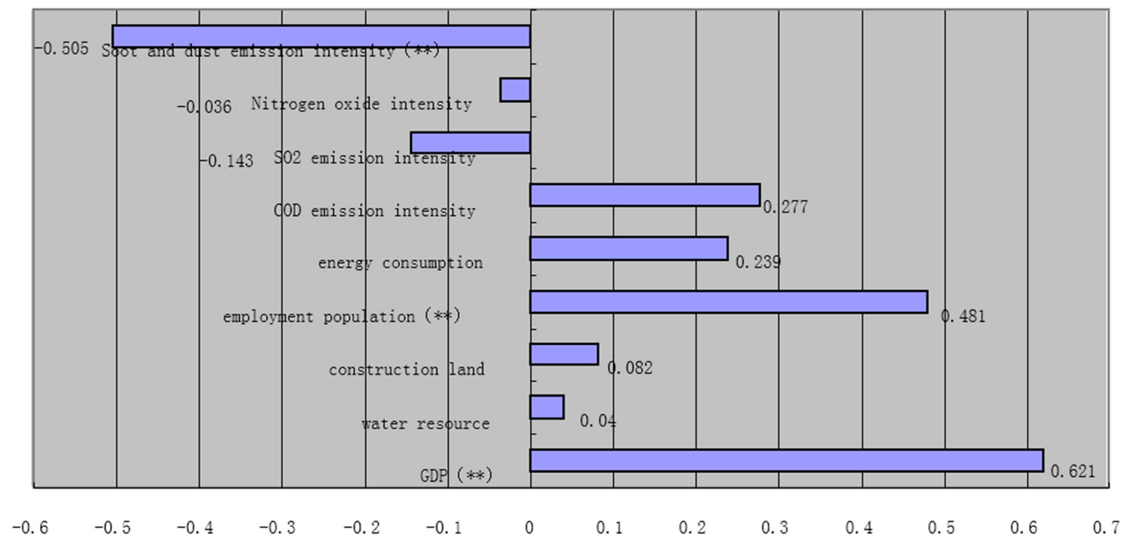
According to the eco-efficiency values $E{E}^{A2}$ of the PSBM model in Table 2, we can obtain the ecological performance value $\eta =(1-E{E}^{A2})$. The greater η is, the better the ecological performance of the DMU is. Figure 1 gives the Spearman rank correlation coefficients between η and each input, desirable output and undesirable output emission intensity (tons per 10 thousand hectares) so that the relationship among them can be analyzed.

Figure 1 shows the greater the GDP and employment population is, the higher the ecological performance is. The smaller the soot and dust emission intensity is, the higher the ecological performance is, which shows, to some extent, the more eco-efficient provinces give some emphasis on cleaner production in recent years while developing the economy.

Since ecological performance might increase even if resource inputs and pollutants emissions increase as long as the desirable outputs expand faster, we cannot judge that the eco-efficient provinces are more sustainable than other provinces. Both central and local governments in China have preferences for GDP growth while neglecting low efficiency resource utilization and environmental degradation. However, this does not render the role of the concept of eco-efficiency. Measurement of eco-efficiency is vital for finding an effective way of decreasing environmental pressures.

4. Discussion

In efficiency assessment, DDFM model is widely used due to its advantages. On the one hand, it generalizes some existing DEA models. For example, input-oriented and output-oriented radial measure models are particular DDFM models under a special directional vector. On the other hand, it is flexible in choosing the directional vector. Although the directional vector is considered arbitrary, some directional vectors reflect the value judgment of decision-makers. The DDFM model under the vector of input and output can provide the improved proportion of each indicator. Compared to the observed variables, the evaluation results under the range vector are relative to the maximum inefficiency, which the observations allow in each input and output. The maximum of the input (or undesirable output) is the worst observed value for this input (or undesirable output). The minimum of the desirable output is the worst observed value for this desirable output. However, DDFM model does not take into account the true amount of slack. It only considers the directional slack, whereas non-directional slack is an important source of inefficiency. Hence, this paper investigates the evaluation problem of eco-efficiency by the slacks-based measure model. Based on DDFM model and some slacks-based model, we set up the PSBM and WPSBM models to assess the EE. The proposed model is related to the directional vector, and it is a linear programming, which is solved easily. Moreover, it considers the resource inputs, desirable outputs and undesirable outputs simultaneously and can provide the expanded (decreased) proportion of the desirable output (resource input and pollutant emission). In addition, the decision makers can assign the weights to the slacks of the indicators in the objective function of WPSBM model, according to the economic importance. The empirical study demonstrates that all the efficient units for the proposed PSBM and WPSBM models are the same as those generated by the DDFM model. However, DDFM model overestimated the ecological performance of DMU. Comparing the results of WPSBM model with that of DDFM model, we can find non-directional slack is a vital source of inefficiency and should not be neglected. The WPSBM model takes into account the total slack amount, including the directional slack and non-directional slack. The empirical study indicates, for different directional vectors and any given weight vector, all the efficient DMUs for the DDFM, PSBM and WPSBM models are same. The evaluation results of various directional vectors are different, and the directional vector influences eco-efficiency in WPSBM. The weight impacts on the assessment of the eco-efficiency. In conclusion, the empirical study results indicate the developed slacks-based measure model can be used in the assessment of eco-efficiency effectively and reasonably.

In addition, the evaluation results demonstrate that the eco-efficiency and GDP exhibits highly positive correlation at the 0.01 level in China. One of the reasons is that China’s officeholders are assessed and promoted based on economic growth rather than social and environmental performance, which makes local government emphasize GDP growth with less attention to environmental protection. However, GDP is only one of the important indicators used to measure economic development level. There are other economic development indexes such as per capita disposable income, per capita net income of farmers, power consumption per 10 thousand GDP, the proportion of the third industry population, environment and so on. The computation results also indicate provinces with higher ecological performance use more labor and construction land, and yield higher COD emission intensity. Hence, provinces with higher ecological performance should also increase labor productivity and output of construction land, and decrease COD emission intensity. From the results in Table 4 in the empirical analysis, there is still a greater contraction space for resource input and pollutant emission in china. Totally, regarding inefficient provinces in China, the consumption of water resources should be decreased greatly, as well as construction land and energy consumption. Moreover, the discharge of soot and dust should be reduced sharply, followed by COD and SO₂. In industry, agriculture, service sector and people’s life, water resource and energy consumption should be saved. At the same time, it is important to reduce emissions. Firm, manager, government and the public should realize the importance of environmental protection. In recent years, in China, more and more cities are suffering from smog, which seriously affects people’s life and health. Hence, emission of soot and dust, SO₂, and nitrogen oxide should be decreased sharply. In addition, water pollution often occurs in some areas and water resources are scarce. Our work allows us to draw an important conclusion that central and local government neglect resource utilization efficiency and environmental degradation when developing the economy. However, better resource utilization efficiency is the way to reduce conflicts between future development and resource burdens [62,63,64].

Circular economy and cleaner production should be adopted as one of the strategies to developing the economy in order to protect environment. Circular economy is based upon the 3R principles (reduction, reuse and recycle). Circular economy refers to the transformation of the traditional “resources–products–pollutions” mode into the “resources–products–regenerated resources” mode, which can realize the closed loop of resources and energy flow in social and economy activities [65]. Developing the circular economy is the key to achieve economic development, ecology and environmental protection. The circular economy potentially increases value to business and communities by optimizing the use of materials, energy and community resources. Cleaner production is widely applicable and generally delivers both environmental and competitive advantage, even though the theoretical debate whether being green can be competitive is far from resolved [66]. Cleaner production can improve the eco-efficiency of one company through pollution prevention approach. The circular economy and cleaner production improve resource utilization efficiency, protect the environment and realize sustainable development. The eco-efficiency indicator has been used to measure environmental performance related to economic performance in the application of circular economy. Various areas should have different strategies for higher ecological performance and sustainable development. Central government should provide more technical and financial assistance to less developed areas for improving their eco-efficiency and sustainable development. Moreover, regulation toward pollution control also plays a vital role. In addition, environmental proactivity has a positive and significant effect on the firm’s economic value. It can improve the competitiveness of firms by reducing costs [5]. Hence, environmental proactivity has a greater influence on decreasing environmental pressures (resource consumption and waste emission) and improving eco-efficiency [5]. The notion of eco-efficiency should be widely spread to public, enterprise and government.

Finally, this research has some limitations. Further work needs to be done in these area. First, the input and output indicators should be expanded, such as the total material requirement and cultural indicators, which can analyze eco-efficiency comprehensively. Apart from these indicators, in the feasible conditions, greenhouse gas emissions may be collected or computed approximately by other methods and be taken as one of the undesirable output indicators. Second, the proposed DEA models should be combined with other methods, such as life cycle assessment (LCA). LCA approach can be used to assess the potential environmental impacts and resources used. Third, future empirical research should apply the proposed DEA models to the dynamic analysis of eco-efficiency, which can explain changes of eco-efficiency over time and reflect the region’s sustainable development more accurately. Furthermore, the dual problem of the model should be investigated.

References

- World Commission on Environment and Development (WCED). Our Common Future; Oxford University Press: Oxford, UK, 1987. [Google Scholar]
- Schaltegger, S.; Sturm, A. Okologische rationalitat. Die Unternehm. 1990, 4, 273–290. [Google Scholar]
- Organisation for Economic Co-Operation and Development (OECD). Organization for Economic Cooperation and Development; Eco-Efficiency, OECD: Paris, France, 1998. [Google Scholar]
- World Business Council for Sustainable Development (WBSCD). Eco-Efficiency: Creating More Value with Less Impact; WBSCD: Geneva, Switzerland, 2000. [Google Scholar]
- Barba-Sanchez, V.; Atienza-Sahuquillo, C. Environmental proactivity and environmental and economic performance: Evidence from the winery sector. Sustainability 2016, 8, 1014. [Google Scholar] [CrossRef]
- Zhu, D.J.; Qiu, S.F. Eco-efficiency indicators and their demonstration as the circular economy measurement in China. Resour. Environ. Yangtze Basin 2008, 17, 1–5. [Google Scholar]
- Tian, J.; Wang, C.R.; Lu, G.F. Application of analytic hierarchy process in eco-efficiency assessment. Chin. Environ. Prot. Sci. 2009, 35, 118–120. [Google Scholar]
- Han, R.L.; Tong, L.J.; Song, Y.N. Analysis of circular economy of Liaoning province based on eco-efficiency. Chin. Acta Ecol. Sin. 2011, 31, 4732–4740. [Google Scholar]
- Pan, X.X.; He, Y.Q.; Hu, X.F. Evaluation and spatial econometric analysis on regional ecological efficiency. Chin. Resour. Environ. Yangtze Basin 2013, 22, 640–646. [Google Scholar]
- Korhonen, P.J.; Luptacik, M. Eco-efficiency analysis of power plants: An extension of data envelopment analysis. Eur. J. Oper. Res. 2004, 154, 437–446. [Google Scholar] [CrossRef]
- Hua, Z.S.; Bian, Y.W.; Liang, L. Eco-efficiency analysis of paper mills along the Huai River: An extended DEA approach. Omega 2007, 35, 578–587. [Google Scholar] [CrossRef]
- Zhang, B.; Bi, J.; Yuan, Z.; Yuan, Z.W.; Ge, J.J. Eco-efficiency analysis of industrial system in China: A data envelopment analysis approach. Ecol. Econ. 2008, 68, 306–316. [Google Scholar] [CrossRef]
- Picazo-Tadeo, A.J.; Beltran-Esteve, M.; Gomez-Limon, J.A. Assessing eco-efficiency with directional distance functions. Eur. J. Oper. Res. 2012, 220, 798–809. [Google Scholar] [CrossRef]
- Yin, K.; Wang, R.S.; An, Q.X.; Yao, L.; Liang, J. Using eco-efficiency as an indicator for sustainable urban development: A case study of Chinese provincial capital cities. Ecol. Indic. 2014, 36, 665–671. [Google Scholar] [CrossRef]
- Wu, J.; Yin, P.Z.; Sun, J.S.; Chu, J.F.; Liang, L. Evaluating the environmental efficiency of a two-stage system with undesirable outputs by a DEA approach: An interest preference perspective. Eur. J. Oper. Res. 2016, 254, 1047–1062. [Google Scholar] [CrossRef]
- Atienza-Sahuquillo, C.; Barba-Sanchez, V. Design of a measurement model for environmental performance: Application to the food sector. Environ. Eng. Manag. J. 2014, 13, 1463–1472. [Google Scholar]
- Wu, D.X.; Wu, D.D. Performance evaluation and risk analysis of online banking service. Kybernetes 2010, 39, 723–734. [Google Scholar] [CrossRef]
- Chen, H.; Chen, P.; Luo, Y. Eco-efficiency assessment of resource-based cities of China based on super-efficiency DEA model. J. Dalian Univ. Technol. 2015, 36, 34–40. [Google Scholar]
- Guo, C.Z.; Luo, L.L.; Ye, M. Empirical analysis of factors influencing the sustainable development of resource-based cities. China Popul. Resour. Environ. 2014, 24, 81–89. [Google Scholar]
- Hwang, S.N.; Chen, C.; Chen, Y.; Lee, H.S.; Shen, P.D. Sustainable design performance evaluation with applications in the automobile industry: Focusing on inefficiency by undesirable factors. Omega 2013, 14, 553–558. [Google Scholar] [CrossRef]
- Chambers, R.G.; Chung, Y.; Fare, R. Benefit and distance functions. J. Econ. Theory 1996, 70, 407–419. [Google Scholar] [CrossRef]
- Chambers, R.G.; Chung, Y.; Fare, R. Profit, directional distance functions and Nerlovian efficiency. J. Optim. Theory Appl. 1998, 98, 351–364. [Google Scholar] [CrossRef]
- Silva Portela, M.C.A.; Thanassoulis, E.; Simpson, G. Negative data in DEA: A directional distance approach applied to bank branches. J. Oper. Res. Soc. 2004, 55, 1111–1121. [Google Scholar] [CrossRef]
- Picazo-Tadeo, A.J.; Reig-Martinez, E.; Hernandez-Sancho, F. Directional distance functions and environmental regulation. Resour. Energy Econ. 2005, 27, 131–142. [Google Scholar] [CrossRef]
- Picazo-Tadeo, A.J.; Castillo-Gimenez, J.; Beltran-Esteve, M. An intertemporal approach to measuring environmental performance with directional distance functions: Greenhouse gas emissions in the European Union. Ecol. Econ. 2014, 100, 173–182. [Google Scholar] [CrossRef]
- Halkos, G.E.; Tzeremes, N.G. A conditional directional distance function approach for measuring regional environmental efficiency: Evidence from UK regions. Eur. J. Oper. Res. 2013, 227, 182–189. [Google Scholar] [CrossRef]
- Mahlberg, B.; Luptacik, M. Eco-efficiency and eco-productivity change over time in a multisectoral economic system. Eur. J. Oper. Res. 2014, 234, 885–897. [Google Scholar] [CrossRef]
- Pastor, J.T.; Ruiz, J.L.; Sirvent, I. An enhanced Russell graph efficiency measure. Eur. J. Oper. Res. 1999, 115, 596–607. [Google Scholar] [CrossRef]
- Briec, W. An extended Fare-Lovell technical efficiency measure. Int. J. Prod. Econ. 2000, 65, 191–199. [Google Scholar] [CrossRef]
- Charnes, A.; Cooper, W.W.; Golany, B.; Seiford, L. Foundations of data envelopment analysis for Pareto-Koopmans efficient empirical production functions. J. Econom. 1985, 30, 91–107. [Google Scholar] [CrossRef]
- Cooper, W.W.; Park, K.S.; Pastor, J.T. RAM: A range adjusted measure of inefficiency for use with additive models and relations to other models and measures in DEA. J. Prod. Anal. 1999, 11, 5–42. [Google Scholar] [CrossRef]
- Tone, K. A slacks-based measure of efficiency in data envelopment analysis. Eur. J. Oper. Res. 2001, 130, 498–509. [Google Scholar] [CrossRef]
- Fukuyama, H.; Weber, W.L. A directional slacks-based measure of technical inefficiency. Socio-Econ. Plan. Sci. 2009, 43, 274–287. [Google Scholar] [CrossRef]
- Fukuyama, H.; Weber, W.L. A slacks-based inefficiency measure for a two-stage system with bad outputs. Omega 2010, 38, 398–409. [Google Scholar] [CrossRef]
- Gómez-Calvet, R.; Conesa, D.; Gómez-Calvet, A.R.; Tortosa-Ausina, E. On the dynamics of eco-efficiency performance in the European Union. Comput. Oper. Res. 2016, 66, 336–350. [Google Scholar] [CrossRef]
- Sharp, J.A.; Meng, W.; Liu, W. A modified slacks-based measure model for data envelopment analysis with natural negative outputs and inputs. J. Oper. Res. Soc. 2007, 58, 1672–1677. [Google Scholar] [CrossRef]
- Asmild, M.; Pastor, J.T. Slack free MEA and RDM with comprehensive efficiency measures. Omega 2010, 38, 475–483. [Google Scholar] [CrossRef]
- Gómez-Calvet, R.; Conesa, D.; Gómez-Calvet, A.R.; Tortosa-Ausina, E. Energy efficiency in the European Union: What can be learned from the joint application of directional distance functions and slacks-based measures? Appl. Energy 2014, 132, 137–154. [Google Scholar] [CrossRef]
- Picazo-Tadeo, A.J.; Gomez-Limon, J.A.; Reig-Martinez, E. Assessing farming eco-efficiency: A data envelopment analysis approach. J. Environ. Manag. 2011, 92, 1154–1164. [Google Scholar] [CrossRef] [PubMed]
- Kuosmanen, T.; Kortelainen, M. Measuring eco-efficiency of production with data envelopment analysis. J. Ind. Ecol. 2005, 9, 59–72. [Google Scholar] [CrossRef]
- Torgersen, A.; Forsund, F.; Kittelsen, S. Slack-adjusted efficiency measures and ranking of efficient units. J. Prod. Anal. 1996, 7, 379–398. [Google Scholar] [CrossRef]
- Farrell, M.J. The measurement of productive efficiency. J. R. Stat. Soc. 1957, 120, 253–281. [Google Scholar] [CrossRef]
- Forsund, F.R.; Hjalmarsson, L. On the measurement of productive efficiency. Swed. J. Econ. 1974, 76, 141–154. [Google Scholar] [CrossRef]
- Banker, R.D.; Charnes, A.; Cooper, W.W. Some models for estimating technical and scale inefficiencies in Data Envelopment Analysis. Manag. Sci. 1984, 30, 1078–1092. [Google Scholar] [CrossRef]
- Liu, J.; Tone, K. A multistage method to measure efficiency and its application to Japanese banking industry. Socio-Econ. Plan. Sci. 2008, 42, 75–91. [Google Scholar] [CrossRef]
- Mickwitz, P.; Melanen, M. Regional eco-efficiency indicators-a participatory approach. J. Clean. Prod. 2006, 14, 1603–1611. [Google Scholar] [CrossRef]
- Reijnders, L. The factor X debate: Setting targets for eco-efficiency. J. Ind. Ecol. 1998, 2, 13–22. [Google Scholar] [CrossRef]
- United Nations Conference on Trade and Development (UNCTD). Integrating Environmental and Financial Performance at the Enterprise Level: A Methodology for Standardizing Eco-Efficiency Indicators; United Nations Publication: New York, NY, USA, 2003; pp. 29–30. [Google Scholar]
- Seppäläa, J.; Melanen, M.; Mäenpää, I.; Koskela, S.; Tenhunen, J.; Hiltunen, M.R. How can the eco-efficiency of a region be measured and monitored? J. Ind. Ecol. 2005, 9, 117–130. [Google Scholar] [CrossRef]
- De Leeuw, F.A. A set of emission indicators for long-range transboundary air pollution. Environ. Sci. Policy 2002, 5, 135–145. [Google Scholar] [CrossRef]
- Mahlberg, B.; Sahoo, B.K. Radial and non-radial decompositions of Luenberger productivity indicator with an illustrative application. Int. J. Prod. Econ. 2011, 131, 721–726. [Google Scholar] [CrossRef]
- Kortelainen, M. Dynamic environmental performance analysis: A Malmquist index approach. Ecol. Econ. 2008, 64, 701–715. [Google Scholar] [CrossRef]
- Verfaillie, H.A.; Bidwell, R. Measuring Eco-Efficiency: A Guide to Reporting Company Performance; World Business Council for Sustainable Development: Geneva, Switzerland, 2000. [Google Scholar]
- Yin, K.; Wang, R.S.; Yao, L.; Liang, J. The eco-efficiency evaluation of the model city for environmental protection in China. Acta Ecol. Sin. 2011, 31, 5588–5598. [Google Scholar]
- Egilmez, G.; Kucukvar, M.; Tatari, O. Sustainability assessment of U.S. manufacturing sectors: An economic input output-based frontier approach. J. Clean. Prod. 2013, 53, 91–102. [Google Scholar] [CrossRef]
- Sorvari, J.; Antikainen, R.; Kosola, M.L.; Hokkanen, P.; Haavisto, T. Eco-efficiency in contaminated land management in Finland-barriers and development needs. J. Environ. Manag. 2009, 90, 1715–1727. [Google Scholar] [CrossRef] [PubMed]
- Topa, G. Social interactions, local spillovers and unemployment. Rev. Econ. Stud. 2001, 68, 261–295. [Google Scholar] [CrossRef]
- Oggioni, G.; Riccardi, R.; Toninelli, R. Eco-efficiency of the world cement industry: A data envelopment analysis. Energy Policy 2011, 39, 2842–2854. [Google Scholar] [CrossRef]
- Song, M.L.; Wang, S.H.; Liu, Q.L. Environmental efficiency evaluation considering the maximization of desirable outputs and its application. Math. Comput. Model. 2013, 58, 1110–1116. [Google Scholar] [CrossRef]
- Sueyoshi, T.; Goto, M. Measurement of returns to scale and damages to scale for DEA-based operational and environmental assessment: How to manage desirable (good) and undesirable (bad) output? Eur. J. Oper. Res. 2011, 211, 76–89. [Google Scholar] [CrossRef]
- Wu, M.R.; Ma, J. Measurement on regional ecological efficiency in China and analysis on its influencing factors: Based on DEA-Tobit two stage method. Technol. Econ. 2016, 35, 75–80. [Google Scholar]
- Wu, H.Q.; Shi, Y.; Xia, Q.; Zhu, W.D. Effectiveness of the policy of circular economy in China: A DEA-based analysis for the period of 11th five-year-plan. Resour. Conserv. Recycl. 2014, 83, 163–175. [Google Scholar] [CrossRef]
- Yu, C.J.; Li, H.Q.; Jia, X.P.; Li, Q. Improving resource utilization efficiency in China’s mineral resource-based cities: A case study of Chengde, Hebei province. Res. Conserv. Recycl. 2015, 94, 1–10. [Google Scholar] [CrossRef]
- Yune, J.H.; Tian, J.P.; Liu, W.; Chen, L.J.; Descamps-Large, C. Greening Chinese chemical industrial park by implementing industrial ecology strategies: A case study. Resour. Conserv. Recycl. 2016, 112, 54–64. [Google Scholar] [CrossRef]
- Mathews, J.A.; Tan, H. Progress toward a circular economy in China. J. Ind. Ecol. 2011, 15, 435–457. [Google Scholar] [CrossRef]
- Howgrave-Graham, A.; Berkel, R.V. Assessment of cleaner production uptake: Method development and trial with small businesses in Western Australia. J. Clean. Prod. 2007, 15, 787–797. [Google Scholar] [CrossRef]
Figure 1.
Spearman rank correlation coefficients between (Table 2) and input, desirable output, and undesirable output emission intensity (tons per 10 thousand hectares). Note: **: p < 0.01.