Wind Speed for Load Forecasting Models

Abstract

Temperature and its variants, such as polynomials and lags, have been the most frequently-used weather variables in load forecasting models. Some of the well-known secondary driving factors of electricity demand include wind speed and cloud cover. Due to the increasing penetration of distributed energy resources, the net load is more and more affected by these non-temperature weather factors. This paper fills a gap and need in the load forecasting literature by presenting a formal study on the role of wind variables in load forecasting models. We propose a systematic approach to include wind variables in a regression analysis framework. In addition to the Wind Chill Index (WCI), which is a predefined function of wind speed and temperature, we also investigate other combinations of wind speed and temperature variables. The case study is conducted for the eight load zones and the total load of ISO New England. The proposed models with the recommended wind speed variables outperform Tao’s Vanilla Benchmark model and three recency effect models on four forecast horizons, namely, day-ahead, week-ahead, month-ahead, and year-ahead. They also outperform two WCI-based models for most cases.

1. Introduction

During the past decades, researchers have tried many statistical and artificial intelligence techniques to improve load forecasting accuracy [1,2,3,4]. Various load forecasting competitions have also helped recognize some effective techniques and methodologies [5,6,7,8,9,10]. Recently, the load forecasting community has expanded the investigation into some new problems, such as hierarchical load forecasting [7], retail load forecasting [11], and probabilistic load forecasting [2,8,10,12]. No matter which branch of the load forecasting problem, weather variables are included in most models.

Among the various weather variables, the temperature variable is the most entrenched one in the load forecasting literature. In the summer, load increases as temperature increases due to cooling needs. In the winter, load increases as temperature decreases to meet the heating needs. Commonly-used temperature variables are the various forms of dry bulb temperature, such as the piecewise form [13], polynomial [9,10,11,12], and high-order regression splines [14]. The computing power today also allows the inclusion of many lagged and moving average temperature variables, as recently proposed in [15].

Several other adjusted temperature variables, such as wet bulb temperature, dew point temperature, and Temperature-Humidity Index (THI), are also of great interest to the load forecasting community. These variables have the temperature adjusted with humidity information. A formal study on humidity variables for load forecasting models was recently reported in [16], showing that splitting relative humidity and temperature results in more accurate load forecasts than using the predefined THI formula. That sets an example for systematically investigating those secondary weather variables for load forecasting.

Following a similar analytical framework as in [16], this paper fills a gap and need in the load forecasting literature by presenting a formal study on the role of wind variables in load forecasting models. The motivation mainly comes from the fact that the net load is more and more affected by the increased penetration of wind power resources. It gradually becomes a necessity to understand the effect of wind variables in electricity demand to accurately forecast the load. Although wind speed information has been used for load forecasting models [17,18], it is usually embedded in the Wind Chill Index (WCI) or wind speed adjusted temperature [4,17,18,19,20]. Overall, the load forecasting literature on wind speed variables is far less common and thorough than the ones on temperature and relative humidity. The research question we try to answer in this paper is “will splitting wind speed and temperature result in more accurate load forecasts than using the predefined and well-established WCI formula?” If the answer is yes, the follow-up question is “what wind speed variables shall we include in a load forecasting model?”

The rest of this paper is organized as follows: Section 2 introduces the background of this study, including the base models, WCI, and the forecast evaluation techniques; Section 3 presents the exploratory analysis on the case study data; Section 4 discusses the proposed models and the models for comparison; Section 5 presents the results and discussions. The paper is then concluded in Section 6 with a brief discussion of future research.

2. Background

2.1. Multiple Linear Regression Models for Load Forecasting

Multiple linear regression (MLR) is a widely-deployed load forecasting technique in the field due to its transparency, interpretability, and simplicity. In this paper, we will use MLR models for the analysis due to the same reasons. Tao’s Vanilla Benchmark model is a frequently-cited regression model for load forecasting. It was used in GEFCom2012 as the benchmark model [7], and then reproduced by other scholars [21,22]. The model is specified as in Equation (1):

$$y_t={\beta }_0+{\beta }_{1}Tren{d}_t+{\beta }_2{M}_t+{\beta }_3{W}_t+{\beta }_4{H}_t+{\beta }_5{W}_t{H}_t+f(T_t)$$

(1)

where y_t is the expected load; Trend_t is a chronological trend at time t; M_t, W_t and H_t are class variables for month, day of a week, and hour of a day at time t; and T_t is the coincidence temperature. Let $f(T_t)$ be defined as in Equation (2):

$$f(T_t)={\alpha }_1{T}_t+{\alpha }_2{T}_t^2+{\alpha }_3{T}_t^3+{\alpha }_4{T}_t{M}_t+{\alpha }_5{T}_t^2{M}_t+{\alpha }_6{T}_t^3{M}_t+{\alpha }_7{T}_t{H}_t+{\alpha }_8{T}_t^2{H}_t+{\alpha }_9{T}_t^3{H}_t$$

(2)

Furthermore, considering the impact of lagged temperature on load, we can add the various forms of lagged temperature variables to the benchmark model as in Equation (3):

$$y_t={\beta }_0+{\beta }_{1}Trend+{\beta }_2{M}_t+{\beta }_3{W}_t+{\beta }_4{H}_t+{\beta }_5{W}_t{H}_t+{\sum }_{h}f(T_{t-h})+{\sum }_{d}f({\tilde{T}}_{t,d})$$

(3)

where T_t−h is the temperature of previous h^th hours (h = 0, 1, 2, …); ${\tilde{T}}_{t,d}=\frac{1}{24}{\sum }_{h=24d-23}^{24d}{T}_{t-h}$ is the 24-h moving average temperature of the previous d^th day (d = 0, 1, 2, …). These models are also known as recency effect models [15]. In this paper, we consider the benchmark model and three variations of the recency effect models to show the effectiveness of including the wind variables in load forecasting models with different levels of sophistication. Specifically, h ranges from 0 to 2; d is up to 1.

2.2. Wind Chill Index

WCI is defined by the National Oceanic and Atmospheric Administration (NOAA) National Weather Service (NWS) to measure how cold people feel in cold and windy weather. It is a predefined function of temperature and wind speed variables describing how the body feels on exposed skin due to the flow of air. The parameters are estimated based on the tests conducted with human subjects [23]. WCI is only defined when the temperature is lower than 50 °F with the wind speed greater than 3 mph. As shown in Equation (4), for cold and windy weather, we follow the WCI defined by NWS. Otherwise, we set it to be equal to the temperature.

$${WCI}_t=\{\begin{array}{l}35.74+0.6125\times T_t-35.75\times W{S}_t^{0.16}+0.4275\times T_t\times W{S}_t^{0.16}, if T_t<50 °\mathrm{F} and W{S}_t>3 mph\\ \hspace{0.5em}{T}_t,\hspace{0.5em}\hspace{1em}\hspace{1em}\hspace{1em}\hspace{1em}\hspace{1em}\hspace{1em}\hspace{1em}\hspace{1em}\hspace{1em}\hspace{1em}\hspace{1em}\hspace{1em}\hspace{1em}\hspace{1em}\hspace{1em}\hspace{1em}\hspace{1em}\hspace{1em}\hspace{1em}\hspace{1em}\hspace{1em}else\end{array}$$

(4)

2.3. Cross-Validation

Cross-validation is a commonly used forecast evaluation technique to avoid potential overfitting issues of a forecasting model [24]. In this paper, we adopt the V-fold cross-validation (VFCV) technique for variable selection, where V is the number of the validation periods. Specifically, the data is first dissected into V pieces with approximately equal size. Every time, we use one of them for validation and the other (V – 1) pieces for model training. This process is repeated V times, one for each validation period. The performance of the model is evaluated based on the average performance of the model on the V validation periods. In Section 4, we will use the three-fold cross-validation to select the wind variables for load forecasting models.

2.4. Out-of-Sample Test

In this paper, we use a sliding simulation with a fixed-length of history to test the forecast accuracy of the models [25]. Sliding simulation keeps rolling the forecast origin forward by the size of the predefined forecast horizon and uses the predefined-length of history prior to the forecast origin for parameter estimation. For example, when we forecast the load one day ahead, we estimate the parameters of the model using a predefined length of the history (e.g., three years) prior to the forecast origin to forecast the next day. This process is repeated by moving the forecast origin one day at a time until we provide the day-ahead forecast for every day of the test year. Alternatively, when the forecast horizon is one month, we repeat the process by moving the forecast origin one-month ahead at a time until we provide the month-ahead forecast for every month of the test year. In Section 5, we will present the performance of the models for day-ahead (e.g., 24-h-ahead, to be specific), week-ahead, month-ahead, and year-ahead forecasting. We test the performance of the models for different forecast horizons to show that the proposed model is not restricted to short- or long-term load forecasting.

3. Data

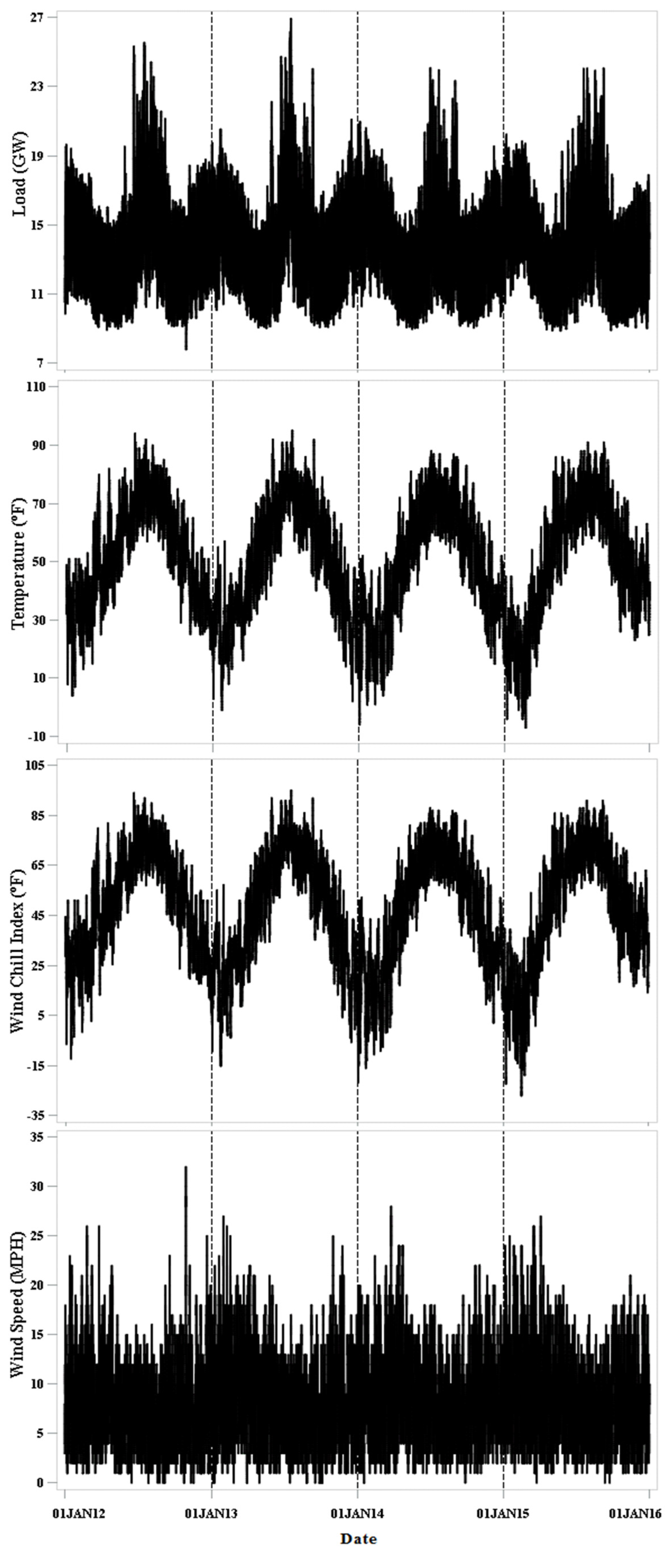
3.1. Data Description

ISO New England (ISONE) is an independent regional transmission organization, serving the six states in the Northeastern United States, including Connecticut (CT), most of Maine (ME), Massachusetts (MA), New Hampshire (NH), Rhode Island (RI), and Vermont (VT). The state of Massachusetts is further dissected into three load zones, namely NEMASS, SEMASS, and WCMASS. Each of the other five states forms its own load zone. ISONE publishes the zonal level hourly load on its website [26]. In this paper, the weather variables, including temperature and wind speed, were provided by a weather service vendor AccuWeather, Inc, State College, PA, USA.

In this paper, we use the system total data of ISONE for demonstration purposes. We present the results of the eight load zones and the system total in Section 5. For each zone, we use the weather data from the closest major airport. For ISONE, we use the average of the weather data from all eight zones. The data being used in this study ranges from 2012 to 2015. The first three years (2012–2014) are used for variable selection based on the three-fold cross-validation, while 2015 is used for out-of-sample tests.

Table 1. Summary statistics of ISONE load zones and system total (2012–2015).

Zone	Weather Station	Load (MW)		Temperature (°F)		WCI (°F)		Wind Speed (MPH)
		Mean	STD.	Mean	STD.	Mean	STD.	Mean	STD.
CT	KBDL	3516.14	766.52	51.61	19.44	49.17	22.31	7.32	5.20
ME	KPWM	1320.56	202.01	47.80	18.57	44.86	21.81	7.40	5.21
NEMASS	KBOS	2914.24	571.68	52.08	17.95	48.79	21.86	10.47	2.33
NH	KCON	1331.56	265.15	47.45	20.35	45.21	22.86	5.45	5.24
RI	KPVD	934.15	202.94	52.17	18.20	49.62	21.30	8.41	5.23
VT	KBTV	653.32	106.66	47.95	21.28	44.91	24.62	7.55	5.55
SEMASS	KPVD	1711.79	387.60	52.17	18.20	49.62	21.30	8.41	5.23
WCMASS	KORH	1980.58	379.29	48.69	18.99	44.81	23.30	9.92	5.06
ISONE	N/A	14,362.35	2825.33	50.05	18.85	46.96	22.39	8.18	4.11

presents the summary statistics of the load and weather data for these four years. There is no pre-processing of data other than the adjustment of the load data for daylight savings time (DST). At the beginning of the DST, we take the average of the adjacent two readings as the load. At the end of the DST, we divide the load by two.

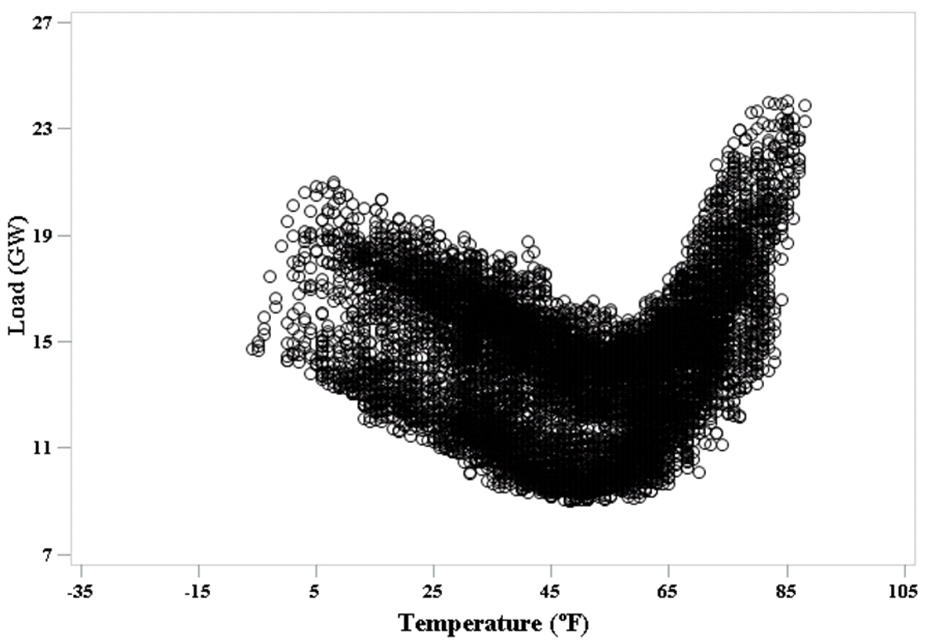
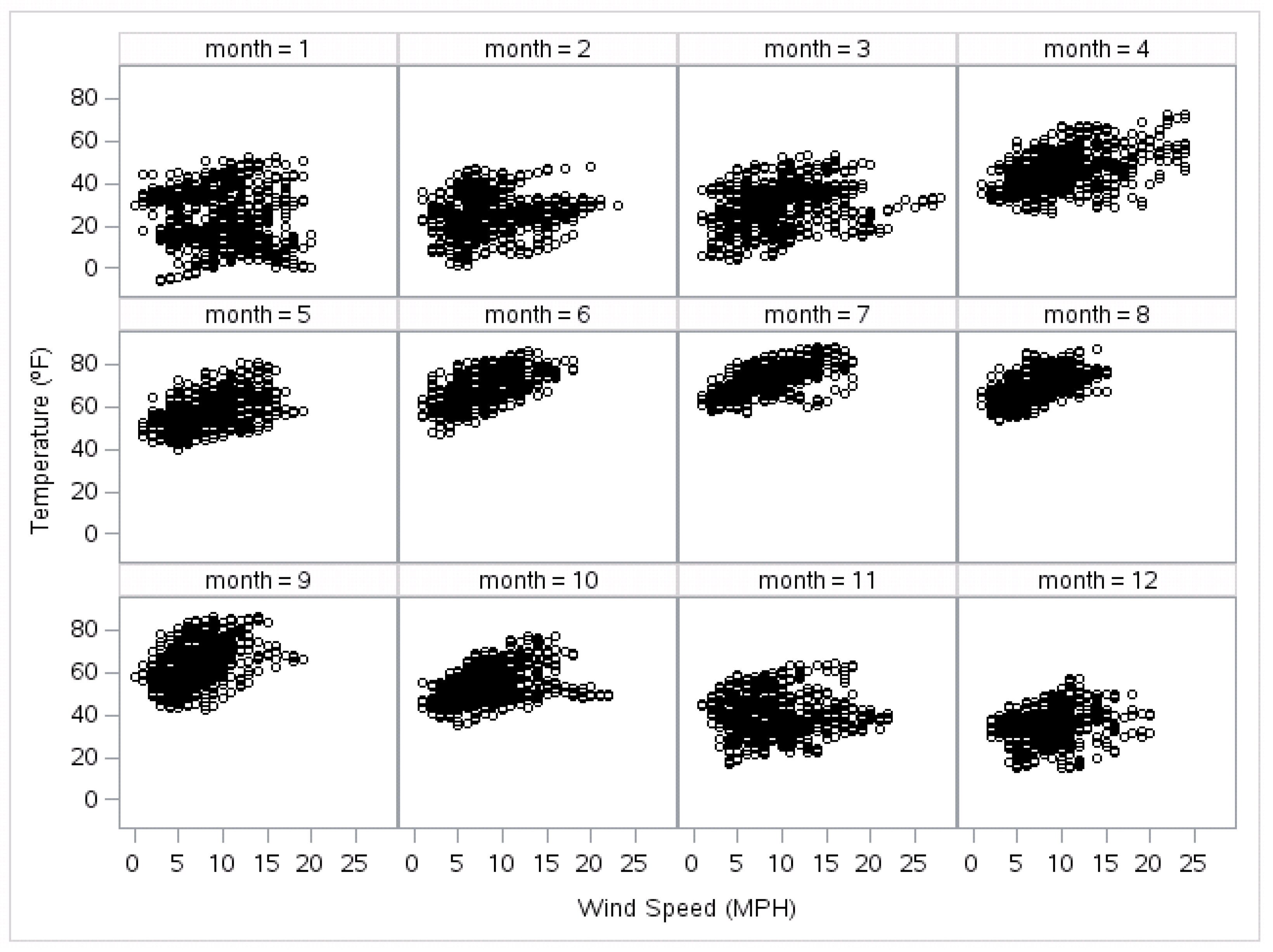
3.2. Exploratory Data Analysis

Figure 1 shows the time series plots of hourly load, temperature, WCI, and wind speed at the system level from 2012 to 2015. Temperature and WCI share a similar seasonal pattern: high in the summer and low in the winter. When WCI is defined (usually in winter months), it is always lower than the temperature and has a wider range. Wind speed varies from 0 to 30 mph during winter months, while the range is much narrower during summer months.

Figure 2 shows the scatterplot between load and temperature, while Figure 3 shows the scatterplot between load and WCI, both in 2014. In this paper, we use the data from the year 2014 for demonstration purposes to avoid verbose presentation, noting that data from other years present similar patterns. When the temperature is higher than 50 °F, WCI is equal to the temperature. In other words, the right arms of the two scatterplots in Figure 2 and Figure 3 are identical. Other than the right arms, the load-WCI scatter is sparser than the load-temperature scatter.

Figure 4 shows the scatterplots between load and wind speed by month during 2014. The correlation between the two variables in June to August is stronger than that in the other months. During these three summer months, load tends to increase when wind speed increases. In the other nine months, the relationship between the two is weak. This appears to be opposite to our common sense that under the same temperature in the summer, the wind makes us feel cooler. For a further investigation, we draw the scatterplots between temperature and wind speed in Figure 5, which suggests a positive correlation between these two variables for most of the months during a year, with the correlation in the summer months being strongest of all. In other words, the counterintuitive observation mentioned above is due to the fact that the load-temperature relationship is much stronger than the load-wind relationship.

To sum up, the four time series plots in Figure 1 depict the seasonal features of load, temperature, WCI, and wind speed. Scatterplots in Figure 2 and Figure 3 show the similar impact of temperature and WCI have on load. Scatterplots of load and wind speed by month in Figure 4 suggest that there is a strong correlation between load and wind speed during the summer months June to August, though some of the correlation is due to the load-temperature relationship and the positive correlation between temperature and wind speed as shown in Figure 5. For the rest of the paper, these three months are defined as summer months. The relationship between wind speed and load for these summer months will be further investigated.

4. Models

4.1. Wind Speed-Related Variables

Due to the strong relationship between load and wind speed during the summer months (i.e., June to August), we introduce the dummy variable S as in (5):

$$S=\{\begin{array}{l}1, June, July, or August\\ 0, else\end{array}$$

(5)

This dummy variable S is equal to 1 if the month is June, July, or August, and 0 otherwise. We use WSS_t to denote the coincidence wind speed in summer.

For each of the four base models defined in Section 2, we introduce the wind speed variables in the following sequence: (1) $WS{S}_t^{0.16}$; (2) $T_t\times WS{S}_t^{0.16}$; and (3) $H_t\times WS{S}_t^{0.16}$. Note that we keep the power of 0.16 for wind speed to be consistent with the NWS definition. We then calculate the mean absolute percentage error (MAPE) values as defined in Equation (6) in the three-fold cross-validation setting:

$$MAPE= {{\displaystyle \sum }}_{i=1}^n|\frac{Actua{l}_i-Predic{t}_i}{Actua{l}_i}|$$

(6)

where n is the total number of observations.

The simple average MAPE of the three validation years for all base models and the models with additional wind speed variables are listed in

Table 2. MAPE (%) of base models with additional wind speed terms.

Base Model (h,d)	None	$\mathit{W}\mathit{S}{\mathit{S}}_{\mathit{t}}^{0.16}$	$\mathit{W}\mathit{S}{\mathit{S}}_{\mathit{t}}^{0.16}$ ${\mathit{T}}_{\mathit{t}}\times \mathit{W}\mathit{S}{\mathit{S}}_{\mathit{t}}^{0.16}$	$\mathit{W}\mathit{S}{\mathit{S}}_{\mathit{t}}^{0.16}$ ${\mathit{T}}_{\mathit{t}}\times \mathit{W}\mathit{S}{\mathit{S}}_{\mathit{t}}^{0.16}$ ${\mathit{H}}_{\mathit{t}}\times \mathit{W}\mathit{S}{\mathit{S}}_{\mathit{t}}^{0.16}$
B1(h = 0, d = 0)	3.669	3.666	3.671	3.639
B2(h = 0, d = 1)	3.066	3.061	3.055	3.028
B3(h = 1, d = 1)	2.977	2.971	2.962	2.941
B4(h = 2, d = 1)	2.959	2.953	2.941	2.924

. The None column corresponds to the MAPEs of the models without the wind speed variables. The other three columns present the MAPEs of the models with different sets of wind speed variables. The cooler the background color of the cell is, the better the forecasts are. We can observe that for all four base models, the best results are obtained by using all three recommended effects.

Let $G\left(T_t\right)$ represents a base model depending upon temperature variables; we define the proposed model family as in Equation (7):

$$y_t=G\left(T_t\right)+g\left(W{S}_t\right)$$

(7)

where:

$$g\left(W{S}_t\right)={\gamma }_{1}WS{S}_t^{0.16}+{\gamma }_2{T}_t\times WS{S}_t^{0.16}+{\gamma }_3{H}_t\times WS{S}_t^{0.16}$$

(8)

Comparing with the NWS’s formula for WCI (Equation (4)), the proposed Equation (8) extends the WCI (Equation (4)) by adding interactions between wind speed and dummy variable S, and between wind speed and hour. Furthermore, the proposed model allows the parameters to be estimated based on the dataset, while the parameters in Equation (4) are predefined.

4.2. Two WCI-Based Models

Since WCI can be seen as an adjustment to the temperature, we can obtain the first WCI-based model as in Equation (9) by replacing temperature with WCI in Equation (3):

$$y_t=G\left(WC{I}_t\right)$$

(9)

Another way to include WCI variables is to treat them as the wind speed and replace the wind speed with WCI in Equation (7), which gives us the second WCI-based model (Equation (10)). However, when WCI is less than zero, the WCI terms being used in $g\left(WC{I}_t\right)$ become undefined. In such cases, we leave the WCI as-is without taking the root of 0.16:

$$y_t=G\left(T_t\right)+g\left(WC{I}_t\right)$$

(10)

5. Results and Discussion

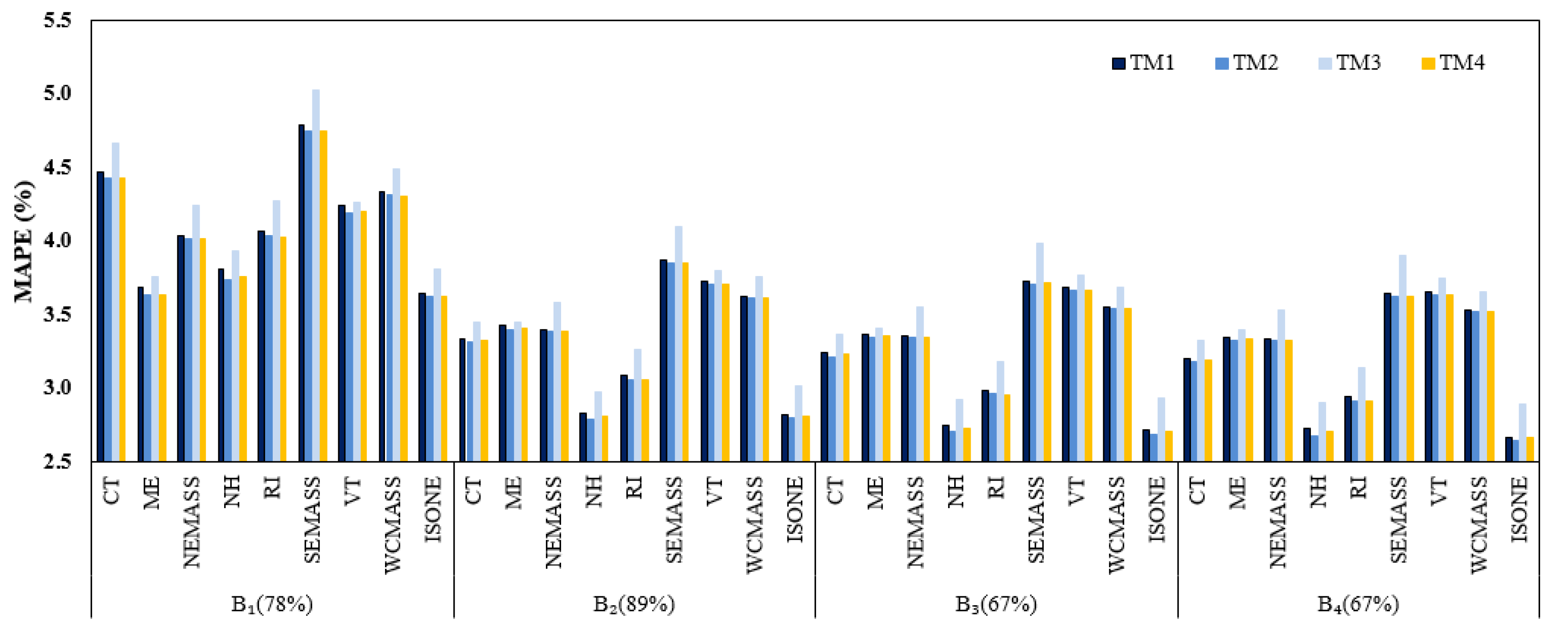
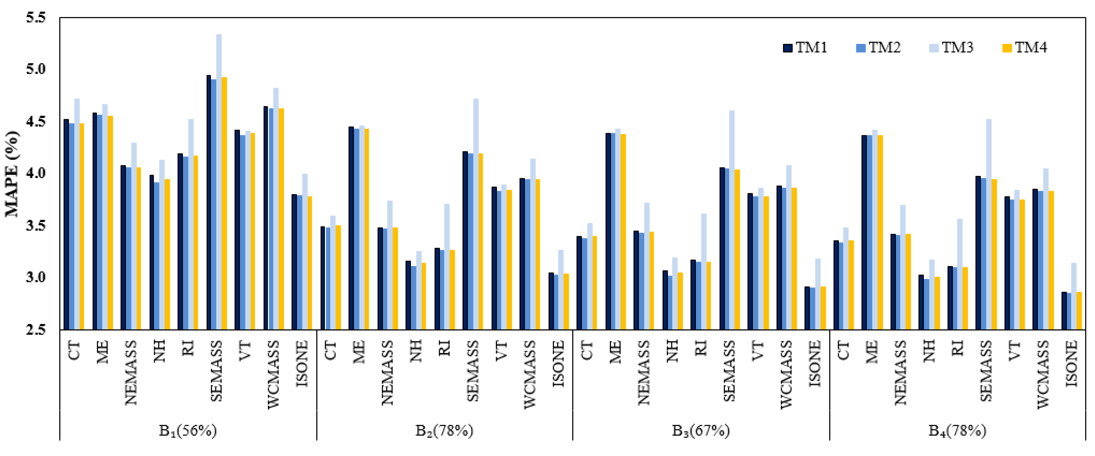
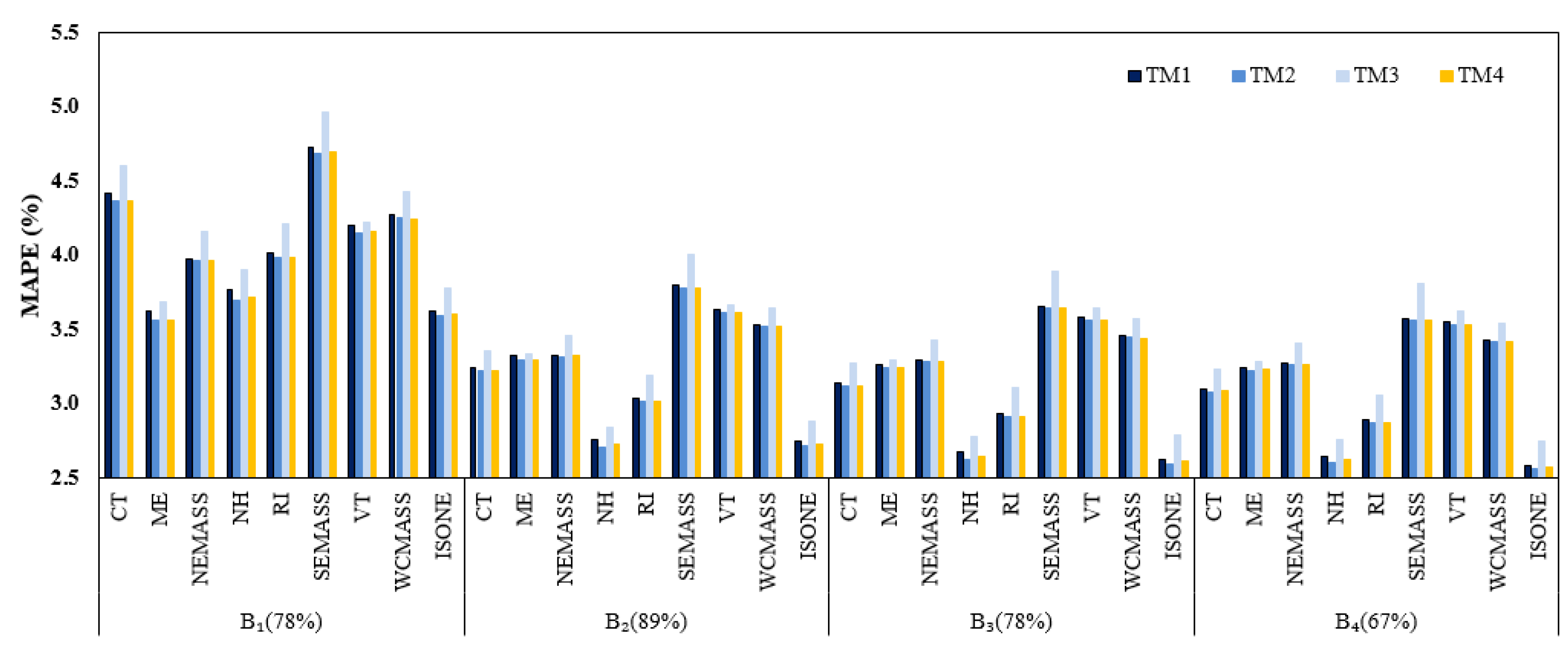
5.1. Out-of-Sample Test

The out-of-sample test is conducted using the data from the year 2015 for all the eight zones and the system. Four forecasting horizons are tested for forecast evaluation: one-day (i.e., 24-h), one-week, one-month, and one-year. For one-week-ahead forecasting, the first seven days of the test year are considered as the first week, the second seven days are considered as the second week, and so on.

The tested model groups are listed in

Table 3. List of tested model groups.

Tested Model Groups	Model Equation
$T{M}_1$	$G\left(T_t\right)$
$T{M}_2$	$G\left(T_t\right)+g\left(W{S}_t\right)$
$T{M}_3$	$G\left(WC{I}_t\right)$
$T{M}_4$	$G\left(T_t\right)+g\left(WC{I}_t\right)$

. They are the base models (TM₁), the base models plus the proposed wind speed terms (TM₂), the base models with WCI replacing the temperature variables (TM₃), and the base models plus the WCI terms (TM₄).

Figure 6, Figure 7, Figure 8 and Figure 9 show the corresponding out-of-sample performance for one-day-ahead, one-week-ahead, one-month-ahead, and one-year-ahead forecasts for all zones across four base models, respectively. Across all of the base models and zones, the proposed TM₂ models outperform the TM₁ models with the relative improvement on MAPE(s) ranging from 0.08% to 1.99%. That confirms the effectiveness of the proposed wind speed variables. On the other hand, TM₃ models are not as accurate as the TM₁ models. In other words, simply replacing temperature with the predefined WCI does not improve the forecast accuracy. Although the TM₄ models also outperform the TM₁ models, the TM₂ models have the lowest MAPE in most cases. The percentage values listed beside the base model label indicates the percentage of the number of zones where TM₂ returns better results than TM₄. In sum, adding the proposed wind speed related variables brings more improvement to the base models on average than using the predefined WCI.

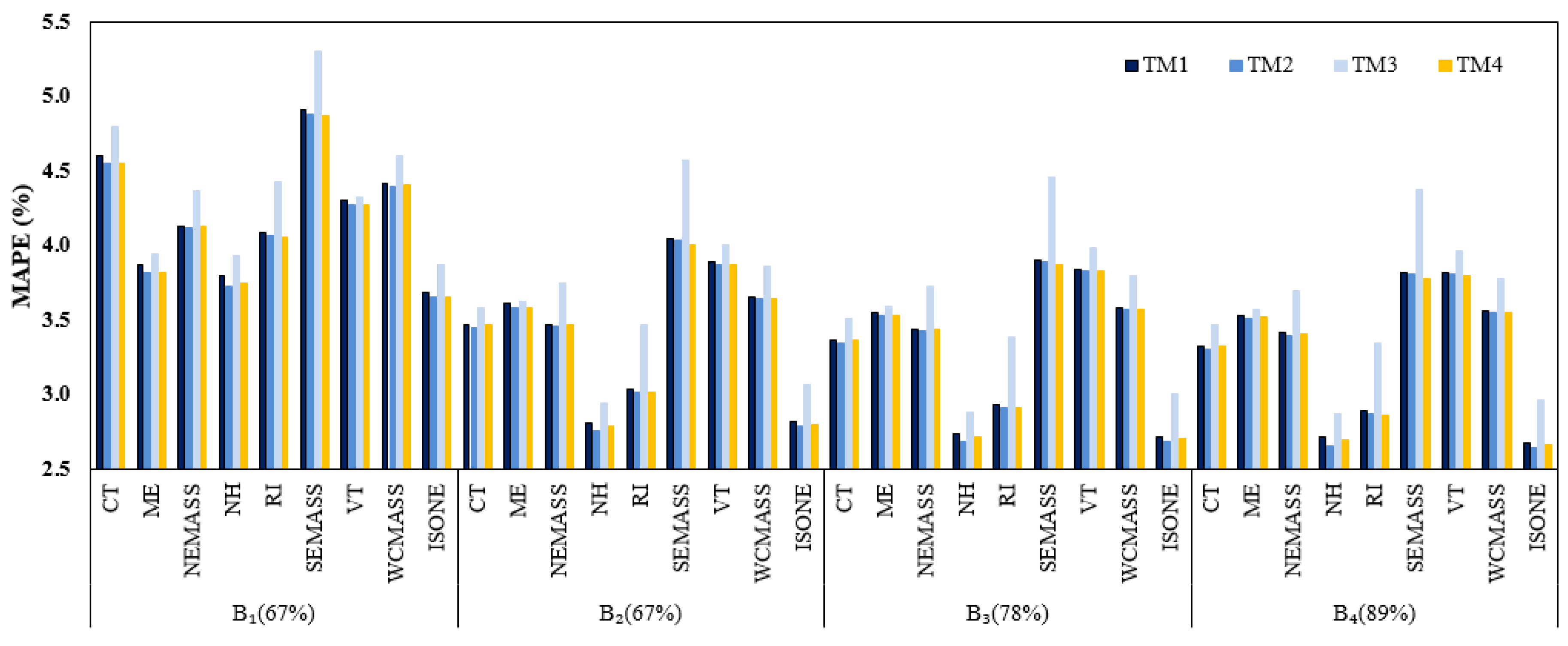
5.2. Ex Ante Forecasting

In this paper, all of the tests have been conducted in the ex post forecasting settings, where the actual weather information is provided through the forecast horizon. In practice, actual weather information is unknown, so the predicted values have to be used to forecast the load. While temperature forecasts nowadays for the short-run are quite accurate, other weather variables, such as wind speed and relative humidity, are not as predictable. Although our empirical case study shows that using the proposed wind speed terms for short-term load forecasting could improve the forecast accuracy, it may or may not help with the ex ante forecast accuracy depending on how accurate the wind speed forecast is. Considering the trade-off between the improvement brought in by using the wind speed variables and the error introduced by the wind speed forecasts, additional empirical studies would be beneficial to tell whether using wind speed variables could benefit the ex ante forecast.

Beyond a few weeks ahead, all weather variables are unpredictable. In recent practices, simulated temperature scenarios have been fed into point load forecasting models to generate probabilistic load forecasts [10,12]. Adding wind speed variables should improve the efficacy of the probabilistic forecast by expanding the range of the scenarios considered. Furthermore, Xie and Hong [27] also demonstrated the effectiveness of relying on point forecast accuracy to select the underlying model for temperature scenario-based probabilistic load forecasts. While this paper offers empirical evidence that the inclusion of the proposed wind variable terms helps reduce point forecast error, additional empirical case studies can be conducted to test the effectiveness of adding wind speed scenarios for probabilistic load forecasting.

5.3. Future Research Directions

In this paper, we formally and systematically study the wind speed variables for load forecasting using models with different comprehensive levels. One future research topic on wind speed variables can follow the similar direction as what was done for the temperature variables in [15] to include lagged and moving-average wind speed variables into the model. Once these wind speed variables are thoroughly studied, the investigation can be extended to net load forecasting with significant wind penetration.

The climate of a relatively small area may differ from that of the surrounding areas, especially when we are looking at weather variables, such as wind speed and cloud cover. Incorporating additional weather variables could potentially help better forecasting the load of a small area. This will require precisely selecting weather stations for the small area. The weather station selection methodology proposed in [28] can be extended with the inclusion of other weather variables. The research conducted in this paper also lays the groundwork for hierarchical load forecasting.

6. Conclusions

In this paper, we investigated the effect of wind on electricity demand using the data from ISONE. Three wind speed-related terms were proposed by looking at the cross-validation MAPE. The out-of-sample tests showed that the proposed wind speed-related variables help improve the temperature-only models and performs better than the WCI defined by NWS in most cases. Researchers can follow the same evaluation process to introduce wind speed variables to load forecasting models for other regions or datasets. The findings in this study also lay the groundwork for several future studies, such as net load forecasting, weather station selection, ex ante short-term load forecasting, probabilistic load forecasting, and hierarchical load forecasting.

References

1. Weron, R. Modeling and Forecasting Electricity Loads and Prices: A Statistical Approach; Wiley Finance: New York, NY, USA, 2006. [Google Scholar]
2. Hong, T.; Fan, S. Probabilistic electric load forecasting: A tutorial review. Int. J. Forecast. 2016, 32, 1–32. [Google Scholar] [CrossRef]
3. Hippert, H.S.; Pedreira, C.E.; Souza, R.C. Neural networks for short-term load forecasting: A review and evaluation. IEEE Trans. Power Syst. 2001, 16, 44–55. [Google Scholar] [CrossRef]
4. Khotanzad, A.; Afkhami-Rohani, R. ANNSTLF—Artificial neural network short-term load forecaster-generation three. IEEE Trans. Power Syst. 1998, 13, 1413–1422. [Google Scholar] [CrossRef]
5. Ramanathan, R.; Engle, R.; Granger, C.W.J.; Vahid-Araghi, F.; Brace, C. Short-run forecasts of electricity loads and peaks. Int. J. Forecast. 1997, 13, 161–174. [Google Scholar] [CrossRef]
6. Chen, B.; Chang, M.; Lin, C. Load forecasting using support vector machines: A study on EUNITE competition 2001. IEEE Trans. Power Syst. 2004, 19, 1821–1830. [Google Scholar] [CrossRef]
7. Hong, T.; Pinson, P.; Fan, S. Global energy forecasting competition 2012. Int. J. Forecast. 2014, 30, 357–363. [Google Scholar] [CrossRef]
8. Hong, T.; Pinson, P.; Fan, S.; Zareipour, H.; Troccoli, A.; Hyndman, R.J. Probabilistic energy forecasting: Global Energy Forecasting Competition 2014 and beyond. Int. J. Forecast. 2016, 32, 896–913. [Google Scholar] [CrossRef]
9. Xie, J.; Liu, B.; Lyu, X.; Hong, T.; Basterfield, D. Combining load forecasts from independent experts. In Proceedings of the 2015 North American Power Symposium, NAPS 2015, Charlotte, NC, USA, 4–6 October 2015. [Google Scholar]
10. Xie, J.; Hong, T. GEFCom2014 probabilistic electric load forecasting: An integrated solution with forecast combination and residual simulation. Int. J. Forecast. 2015, 32, 1012–1016. [Google Scholar] [CrossRef]
11. Xie, J.; Hong, T.; Stroud, J. Long-term retail energy forecasting with consideration of residential customer attrition. IEEE Trans. Smart Grid 2015, 6, 2245–2252. [Google Scholar] [CrossRef]
12. Xie, J.; Hong, T. Temperature scenario generation for probabilistic load forecasting. IEEE Trans. Smart Grid 2016. [Google Scholar] [CrossRef]
13. Fan, S.; Methaprayoon, K.; Lee, W.-J. Multiregion load forecasting for system with large geographical area. IEEE Trans. Ind. Appl. 2009, 45, 1452–1459. [Google Scholar] [CrossRef]
14. Nedellec, R.; Cugliari, J.; Goude, Y. GEFCom2012: Electric load forecasting and backcasting with semi-parametric models. Int. J. Forecast. 2014, 30, 375–381. [Google Scholar] [CrossRef]
15. Wang, P.; Liu, B.; Hong, T. Electric load forecasting with recency effect: A big data approach. Int. J. Forecast. 2016, 32, 585–597. [Google Scholar] [CrossRef]
16. Xie, J.; Chen, Y.; Hong, T.; Laing, T.D. Relative humidity for load forecasting models. IEEE Trans. Smart Grid 2016. [Google Scholar] [CrossRef]
17. McSharry, P.E.; Bouwman, S.; Bloemhof, G. Probabilistic forecasts of the magnitude and timing of peak electricity demand. IEEE Trans. Power Syst. 2005, 20, 1166–1172. [Google Scholar] [CrossRef]
18. Chen, Y.; Luh, P.B.; Guan, C.; Zhao, Y.; Michel, L.D.; Coolbeth, M.A.; Friedland, P.B.; Rourke, S.J. Short-term load forecasting: Similar day-based wavelet neural networks. IEEE Trans. Power Syst. 2010, 25, 322–330. [Google Scholar] [CrossRef]
19. Apadula, F.; Bassini, A.; Elli, A.; Scapin, S. Relationships between meteorological variables and monthly electricity demand. Appl. Energy 2012, 98, 346–356. [Google Scholar] [CrossRef]
20. Ružić, S.; Vučković, A.; Nikolić, N. Weather sensitive method for short term load forecasting in electric power utility of Serbia. IEEE Trans. Power Syst. 2003, 18, 1581–1586. [Google Scholar] [CrossRef]
21. Black, J.D.; Henson, W.L.W. Hierarchical load hindcasting using reanalysis weather. IEEE Trans. Smart Grid 2014, 5, 447–455. [Google Scholar] [CrossRef]
22. Hoverstad, B.A.; Tidemann, A.; Langseth, H.; Ozturk, P. Short-term load forecasting with seasonal decomposition using evolution for parameter tuning. IEEE Trans. Smart Grid 2015, 6, 1904–1913. [Google Scholar] [CrossRef]
23. National Oceanic and Atmospheric Administration. Wind Chill Temperature Index. 2001. Available online: http://www.nws.noaa.gov/om/cold/resources/wind-chill-brochure.pdf (accessed on 14 March 2017).
24. Arlot, S.; Celisse, A. A survey of cross-validation procedures for model selection. Stat. Surverys 2010, 4, 40–79. [Google Scholar] [CrossRef]
25. Tashman, L.J. Out-of-sample tests of forecasting accuracy: An analysis and review. Int. J. Forecast. 2000, 16, 437–450. [Google Scholar] [CrossRef]
26. ISO New England. ISO New England Zonal Information. 2016. Available online: https://www.iso-ne.com/isoexpress/web/reports/pricing/-/tree/zone-info (accessed on 26 October 2016).
27. Xie, J.; Hong, T. Variable selection methods for probabilistic load forecasting: Empirical evidence from seven States of the United States. IEEE Trans. Smart Grid 2017. [Google Scholar] [CrossRef]
28. Hong, T.; Wang, P.; White, L. Weather station selection for electric load forecasting. Int. J. Forecast. 2015, 31, 286–295. [Google Scholar] [CrossRef]
Figure 1. Time series plot of the hourly load, temperature, wind chill index, and wind speed (2012–2015).
Sustainability 09 00795 g001
Figure 2. Scatterplot of the hourly load and temperature (year = 2014).
Sustainability 09 00795 g002
Figure 3. Scatterplot of the hourly load and wind chill index (year = 2014).
Sustainability 09 00795 g003
Figure 4. Scatterplot of hourly load and wind speed by the month of the year (year = 2014).
Sustainability 09 00795 g004
Figure 5. Scatterplot of hourly temperature and wind speed by the month of the year (year = 2014).
Sustainability 09 00795 g005
Figure 6. MAPEs (%) of tested data for one-day-ahead forecasting.
Sustainability 09 00795 g006
Figure 7. MAPEs (%) of tested data for one-week-ahead forecasting.
Sustainability 09 00795 g007
Figure 8. MAPEs (%) of tested data for one-month-ahead forecasting.
Sustainability 09 00795 g008
Figure 9. MAPEs (%) of tested data for one-year-ahead forecasting.
Sustainability 09 00795 g009